High Resolution Photoexcitation Measurements Exacerbate
the Long-standing Fe xvii Oscillator Strength Problem

Abstract

For more than 40 years, most astrophysical observations and laboratory studies of two key soft X-ray diagnostic $2p-3d$ transitions, 3C and 3D, in Fe XVII ions found oscillator strength ratios $f(\mathrm{{3C}})/f(\mathrm{{3D}})$ disagreeing with theory, but uncertainties had precluded definitive statements on this much studied conundrum. Here, we resonantly excite these lines using synchrotron radiation at PETRA III, and reach, at a millionfold lower photon intensities, a 10 times higher spectral resolution, and 3 times smaller uncertainty than earlier work. Our final result of $f(\mathrm{{3C}})/f(\mathrm{{3D}})=3.09(8)(6)$ supports many of the earlier clean astrophysical and laboratory observations, while departing by five sigmas from our own newest large-scale ab initio calculations, and excluding all proposed explanations, including those invoking nonlinear effects and population transfers.

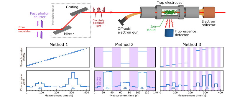
Figure 1: (Top) Experimental setup: an electron beam (orange) aimed at the trap center produces Fe xvii ions, which are then resonantly excited by a monochromatic photon beam (red). Subsequent X-ray fluorescence is registered by a silicon drift detector. (Bottom) Fluorescence yield and photon energy vs. time with three different methods: (1) line scans with open photon shutter; (2,3) by closing it at each step (purple areas), we subtract the electron-beam-induced background at (2) each line center and (3) scanning over a one-full-width-at-half-maximum range.

Space X-ray observatories, such as Chandra and XMM-Newton, resolve $L$-shell transitions of iron dominating the spectra of many hot astrophysical objects Paerels and Kahn (2003); Canizares et al. (2000); Behar et al. (2001); Mewe et al. (2001). Some of the brightest lines arise from Fe xvii (Ne-like iron) around 15 Å: the resonance line 3C ($[(2p^{5})_{1/2}\,3d_{3/2}]_{J=1}\rightarrow[2p^{6}]_{J=0}$) and the intercombination line 3D ($[(2p^{5})_{3/2}\,3d_{5/2}]_{J=1}\rightarrow[2p^{6}]_{J=0}$). Appearing over a broad range of plasma temperatures and densities, they are crucial for diagnostics of electron temperatures, elemental abundances, ionization conditions, velocity turbulences, and opacities Parkinson (1973); Doron and Behar (2002); Xu et al. (2002); Brickhouse and Schmelz (2005); Sanders and Fabian (2011); Kallman et al. (2014); de Plaa et al. (2012); Bailey et al. (2015); Beiersdorfer et al. (2018); Nagayama et al. (2019); Gu, L. et al. (2019). However, for the past four decades, their observed intensity ratios persistently disagree with advanced plasma models, diminishing the utility of high resolution X-ray observations. Several experiments using electron beam ion trap (EBIT) and tokamak devices have scrutinized plausible astrophysical and plasma physics explanations as well as the underlying atomic theory Brown et al. (1998); Beiersdorfer et al. (2001); Brown et al. (2001); Beiersdorfer et al. (2002, 2004); Brown et al. (2006); Brown and Beiersdorfer (2012); Shah et al. (2019), but also revealed clear departures from predictions while broadly agreeing with astrophysical observations Beiersdorfer et al. (2002, 2004); Gu (2009). This has fueled a long-lasting controversy on the cause being a lack of understanding of astrophysical plasmas, or inaccurate atomic data.

A direct probe of these lines using an EBIT at the Linac Coherent Light Source (LCLS) X-ray free-electron laser (XFEL) found again their oscillator strength ratio $f(\mathrm{{3C}})/f(\mathrm{{3D}})$ to be lower than predicted, but close to astrophysical observations Bernitt et al. (2012). This highlighted difficulties with oscillator strengths calculations in many-electron systems Safronova et al. (2001); Chen and Pradhan (2002); Loch et al. (2006); Chen (2007, 2011); Gu (2009); Bernitt et al. (2012); Santana et al. (2015). Nonetheless, at the high peak brilliance of the LCLS XFEL, nonlinear excitation dynamics Oreshkina et al. (2014, 2016) or nonequilibrium time evolution Loch et al. (2015) might have affected the result of Bernitt et al. (2012). An effect of resonance-induced population transfer between Fe xvi and Fe xvii ions was also postulated Wu and Gao (2019) since the Fe xvi line C ($\left[(2p^{5})_{1/2}3s3d_{3/2}\right]_{J=1/2}\to\left[2p^{6}3s\right]_{J=1/2}$) appeared blended with the Fe xvii line 3D. A recent semiempirical calculation Mendoza and Bautista (2017) reproduces the LCLS results Bernitt et al. (2012) by fine-tuning relativistic couplings and orbital relaxation effects, but its validity has been disproved Wang et al. (2017).

In this Letter, we report on new measurements of resonantly excited Fe xvi and Fe xvii with a synchrotron source at tenfold improved spectral resolution and millionfold lower peak photon flux than in Bernitt et al. (2012), suppressing nonlinear dynamical effects Oreshkina et al. (2014); Loch et al. (2015); Li et al. (2017) and undesired ion population transfers Wu and Gao (2019). We also carry out improved large-scale calculations using three different advanced approaches Kozlov et al. (2015); Fischer et al. (2019); Kahl and Berengut (2019), all showing a five-sigma departure from our experimental results.

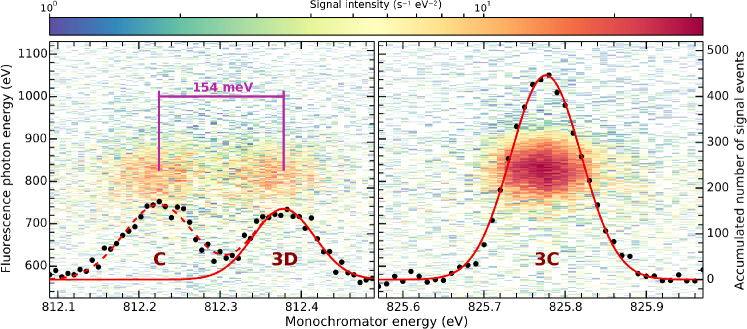
Figure 2: Fluorescence photon yield and energy vs excitation-photon energy for the Fe xvi C, Fe xvii 3C, and 3D transitions recorded by a silicon-drift detector. Black dots: total fluorescence within a 50-eV region of interest. Red solid lines: Fits to 3C and 3D. Red dashed line: fit to C.

We used the compact PolarX-EBIT Micke et al. (2018), in which a monoenergetic electron beam emitted by an off-axis cathode (see Fig. 1) is compressed by a magnetic field. At the trap center, it collides with a beam of iron-pentacarbonyl molecules, dissociating them, and producing highly charged Fe ions with a relative abundance of Fe XVI to Fe XVII close to unity. These ions stay radially confined by the negative space charge of the $\sim$2-mA, 1610-eV ($\approx 3$ times the Fe xvi ionization potential) electron beam, and axially by potentials applied to surrounding electrodes.

Monochromatic, circularly polarized photons from the P04 beamline Viefhaus et al. (2013) at the PETRA III synchrotron photon source enter through the electron gun, irradiate the trapped ions, and exit through the collector aperture. They can resonantly excite X-ray transitions on top of the strong electron-induced background due to ionization, recombination, and excitation processes. A side-on-mounted energy-resolving windowless silicon drift photon detector (SDD) equipped with a 500-nm thin aluminum filter registers these emissions.

By scanning the P04 monochromator between 810 and 830 eV, we excite the Fe xvii lines 3C and 3D, as well as the Fe xvi lines B ($\left[(2p^{5})_{1/2}(3s3d_{3/2})_{1}\right]_{J=1/2}\to\left[2p^{6}3s\right]_{J=1/2}$) and C. They are also nonresonantly excited by electron-impact as the electron beam energy is well above threshold Brown et al. (2006); Shah et al. (2019). This leads to a strong, nearly constant X-ray background at the same energies as the photoexcited transitions but independent of the exciting photon-beam energy. In our earlier work  Bernitt et al. (2012), we rejected this background by detecting the fluorescence in time coincidence with the sub-picosecond-long LCLS pulses of $\approx 10^{11}$ photons each at 120/s. Due to much longer and weaker 50-ps-long pulses ($\approx 10^{3}$ photons, $6\times 10^{6}$/s repetition rate) at P04 and the limited time resolution of SDD, we could not use the coincidence method, and reached a signal-to-background ratio of only $\sim$5%. To improve this, we used a shutter to cyclically turn on and off the P04 photon beam.

Using a 50-$\mu$m slit width, we reached a resolving power of ${E}/{\Delta E}\approx 10000$, ten to fifteen times higher than that of Chandra and XMM-Newton grating spectrometers Den Herder et al. (2001); Canizares et al. (2005), and tenfold that of our previous experiment Bernitt et al. (2012) (See Supplemental Material (SM)). We find a separation of 3C from 3D of $\Delta{E}_{3C-3D}={13.398(1)}~{}{\mathrm{eV}}$, and resolve for the first time the Fe xvii 3D line from the Fe xvi C one at $\Delta{E}_{3D-C}={154.3(1.3)}~{}{\mathrm{meV}}$. This gives us the 3C/3D intensity ratio without having to infer a contribution of Fe xvi line C (in Bernitt et al. (2012) still unresolved) from the intensity of the well-resolved Fe xvi A line. Thereby, we largely reduce systematic uncertainties and exclude the resonance-induced population transfer mechanism Wu and Gao (2019) that may have affected the LCLS result Bernitt et al. (2012).

We apply three different methods (Fig. 1) to systematically measure the 3C/3D oscillator strength ratio. In method 1, we did not operate the photon shutter; instead, we repeatedly scanned the lines C and 3D (812.0 – $812.5\text{\,}\mathrm{eV}$), as well as 3C (825.5 – $826.0\text{\,}\mathrm{eV}$), in both cases using scans of 100 steps with 20-s exposure each (see Fig. 2). The SDD fluorescence signal was integrated over a 50-eV wide photon-energy region of interest (ROI) comprising 3C, 3D, and C, and recorded while scanning the incident photon energy. By fitting Gaussians to the scan result, we obtain line positions, widths, and yields, modeling the electron-impact background as a smooth linear function Shah et al. (2019). The ratio of 3C and 3D areas is then proportional to the oscillator strength ratio Oreshkina et al. (2016). However, given the low 5% signal-to-background ratio and long measurement times, changes in the background cause systematic uncertainties. In method 2, we fixed the monochromator energy to the respective centroids of C, 3D, and 3C found with method 1, and cyclically opened and closed the shutter for equal periods of $20\text{\,}\mathrm{s}$ to determine the background. The background-corrected fluorescence yields at the line peaks were multiplied with the respective linewidths from method 1, to obtain the 3C/3D ratio. Still, slow monochromator shifts from the selected positions could affect the results. To address this, in method 3, we scanned across the FWHM of C, 3D, and 3C in 33 steps with on-off exposures of $20\text{\,}\mathrm{s}$, which reduced the effect of possible monochromator shifts. After background subtraction, we fit Gaussians to the lines of interest fixing their widths to values from method 1.

All three methods share systematic uncertainties caused by energy-dependent filter transmission and detector efficiency ($\sim$1%) and by the incident photon beam flux variation ($\sim$2%). Additionally, for method 1, we estimate systematic uncertainties from background ($\sim$1.2%) and ROI selection ($\sim$2.7%). In method 2, possible monochromator shifts from (set) line centroids and widths taken from method 1 cause a systematic uncertainty of $\sim$3.5%. Analogously, for method 3, we estimate a $\sim$3% uncertainty due to the use of linewidth constraints from method 1. The weighted average of all three methods is $f(\mathrm{3C})/f(\mathrm{3D})=3.09(8)_{\mathrm{sys}}(6)_{\mathrm{stat}}$, see Fig. 3 (see SM for individual ratio and uncertainties). Note that the circular polarization of the photon beam does not affect these results, since 3C and 3D (both ${\Delta}{J}=1$) share the same angular emission characteristics Balashov et al. (2000); Rudolph et al. (2013); Shah et al. (2015, 2018).

Calculations using a density-matrix approach by Oreshkina et al. (2016, 2014), and the time-dependent collisional-radiative model of Loch et al. (2015), pointed to a possible nonlinear response of the excited upper state populations in Bernitt et al. (2012), reducing the observed oscillator strength ratio Li et al. (2017), which would depend on photon pulse parameters, like intensity, duration, and spectral distribution. It has been estimated that peak intensities above 10¹² W/cm² would give rise to nonlinear effects Oreshkina et al. (2014); Li et al. (2017). Fluctuations of the self-amplified spontaneous emission process at LCLS can conceivably generate some pulses above that threshold. At P04, we estimate a peak intensity of $\approx$10⁵ W/cm², more than 6 orders of magnitude below that threshold (see SM). This could explain why the 3C/3D ratio in Bernitt et al. (2012) is in slight disagreement with the present result. Nonetheless, our experiment validates the main conclusion of that work with reduced uncertainty. Our work implies that future experiments at ultra-brilliant light sources should take possible nonlinear effects into account.

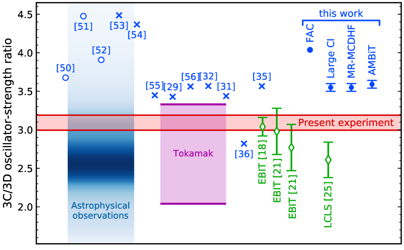
Figure 3: Present experimental 3C/3D ratios compared with previous predictions and experiments. Red band: combined results of the three different methods. Blue open circles: values from databases Kramida et al. (2018); Kaastra et al. (1996); Foster et al. (2012). Blue crosses: predictions Bhatia and Doschek (1992); Chen et al. (2003); Dong et al. (2003); Chen (2007); Oreshkina et al. (2014); Jönsson et al. (2014); Santana et al. (2015); Mendoza and Bautista (2017); Wu and Gao (2019). Note that the validity of theory Mendoza and Bautista (2017) has been disputed Wang et al. (2017). Blue solid circles: present FAC Gu (2008), large-scale CI Kozlov et al. (2015), MR-MCDHF Fischer et al. (2019), and AMBiT Kahl and Berengut (2019) calculations. Blue band: observed line ratios in astrophysical sources Blake et al. (1965); McKenzie et al. (1980); Mewe et al. (2001); Behar et al. (2001); Xu et al. (2002); Ness, J.-U. et al. (2003), with color shades coding the distribution of values weighted by their reported accuracies. Purple band: spread of tokamak results Beiersdorfer et al. (2004). Open green diamonds: previous EBIT results Brown et al. (2001, 2006); Bernitt et al. (2012). Note that the spread seen in various astrophysical sources and in tokamak in part arises from insufficient removal of Fe XVI C line contamination of Fe XVII 3D line, at varying Fe XVI/Fe XVII abundance ratios Doron and Behar (2002); Beiersdorfer et al. (2004); nonlinear dynamical effects Oreshkina et al. (2014); Loch et al. (2015); Li et al. (2017) (see main text) may have reduced the LCLS ratio Bernitt et al. (2012) .

In the present work, we also carried out relativistic calculations using a very-large-scale configuration interaction (CI) method, correlating all ten electrons, including Breit and quantum electrodynamical Tupitsyn et al. (2016) corrections. We implemented a message passing interface (MPI) version of the CI code from  Kozlov et al. (2015) to increase the number of configurations to over 230,000, saturating the computation in all possible numerical parameters. Basis sets of increasing size are used to check for convergence, with all orbitals up to $12sp17dfg$ included in the largest version (the contributions of $n>12\,\,sp$ orbitals are negligible). We start with all possible single and double excitations from the $2s^{2}2p^{6}$, $2s^{2}2p^{5}3p$ even and $2s^{2}2p^{5}3s$, $2s^{2}2p^{5}3d$, $2s2p^{6}3p$, $2s^{2}2p^{5}4d$, $2s^{2}2p^{5}5d$ odd configurations, correlating eight electrons. We separately calculate triple excitations and fully correlate the $1s^{2}$ shell, and also included dominant quadruple ones, finding them negligible. The line strengths $S$ and 3C/3D oscillator strength ratio after several computation stages are summarized in the SM to illustrate the small effect of all corrections. Theoretical uncertainties are estimated based on the variance of results from the smallest to largest runs, size of the various effects, and small variances in the basis set construction. We verified that the energies of all 18 states considered, counted from the ground state, agree with the National Institute for Standards and Technology Kramida et al. (2018) database well within the experimental uncertainty of 0.05%. The theoretical 3C-3D energy difference of 13.44 eV is in agreement with the experiment to 0.3%.

We also carried out entirely independent large-scale calculations using the multireference multiconfiguration Dirac-Hartree-Fock (MR-MCDHF) approach Fischer et al. (2019) with up to 1.2 million configurations. First, the $2s^{2}2p^{5}3s$, $2s^{2}2p^{5}3d$ and $2s2p^{6}3p$ $J=1$ levels were used as reference states to generate the list of configuration state functions with single and double exchanges from all occupied orbitals up to $12spdfghi$. Virtual orbitals were added in a layer-by-layer manner. Subsequently, the role of triple excitations was studied by the CI method. In a second step, the multireference list was extended to include all $J=1$ odd parity states, generated from the Ne-like ground state by single and double electron exchanges. Monitoring the convergence of the results for the addition of layers of virtual orbits, we arrive at an oscillator strength ratio of 3.55(5), and to a 3C-3D energy splitting of 13.44(5) eV. Another full-scale CI calculation with more than a million configurations was carried out in the particle-hole formalism using AMBiT Kahl and Berengut (2019), agreeing well with the other theoretical results. Full details of all calculations can be found in SM.

We emphasize that there are no other known quantum mechanical effects or numerical uncertainties to consider within the CI and MCDHF approaches. With modern computational facilities and MPI codes, we have shown that all other contributions are negligible at the level of the quoted theoretical uncertainties. The significant improvements in experimental and theoretical precision reported here have only further deepened this long-standing problem. This work on the possibly so far most intensively studied many-electron ion in experiment and theory, finally demonstrates convergence of the dedicated atomic calculations on all possible parameters, excluding an incomplete inclusion of the correlation effects as potential explanation of this puzzle.

Our result is the presently most accurate on the 3C/3D oscillator strength ratio. Its excellent resolution suggests promising direct determinations of the natural linewidth. They depend on the Einstein $A$ coefficients, hence, on the oscillator strengths Weisskopf and Wigner (1997). Thus, future accurate measurements of individual natural linewidths of 3C and 3D not only would test theory more stringently than their oscillator strength ratio does, but also deliver accurate oscillator strengths.

Moreover, 3C and 3D with their, among many transitions, strong absorption and emission rates can also dominate the Planck and Rosseland mean opacity of hot plasmas Rogers and Iglesias (1994); Seaton et al. (1994); Beiersdorfer et al. (1996). Therefore, an accurate determination of their oscillator strengths may help elucidating the iron opacity issue Bailey et al. (2007, 2015); Nagayama et al. (2019), if, e. g., Rosseland mean opacity models Fontes et al. (2015); Pain et al. (2017) were found to use predicted oscillator strengths also in departure from experiments. Our result exposes in simplest dipole-allowed transitions of Fe XVII a far greater issue, namely, the persistent problems in the best approximations in use, and calls for renewed efforts in further developing the theory of many-electron systems.

Shortcomings of low-precision atomic theory for $L$-shell ions had already emerged in the analysis of high resolution Chandra and XMM-Newton data Beiersdorfer et al. (2002, 2004); Netzer (2004); Gu (2009); Beiersdorfer et al. (2018). Similar inconsistencies were recently found in the high resolution $K$-shell X-ray spectra of the Perseus cluster recorded with the Hitomi microcalorimeter Hitomi Collaboration et al. (2016, 2018). Moreover, recent opacity measurements Bailey et al. (2015); Nagayama et al. (2019) have highlighted serious inconsistencies in the opacity models used to describe the interiors of stars, which have to rely on calculated oscillator strengths.

All this shows that the actual accuracy and reliability of the opacity and turbulence velocity diagnostics are still uncertain, and with them, the modeling of hot astrophysical and high-energy density plasmas. The upcoming X-ray observatory missions XRISM Tashiro et al. (2018) and  Athena Barret et al. (2016) will require improved and quantitatively validated modeling tools for maximizing their scientific harvest. Thus, benchmarking atomic theory in the laboratory is vital. As for the long-standing Fe xvii oscillator strength problem, our results may be immediately used to semiempirically correct spectral models of astrophysical observations.

High resolution Photoexcitation Measurements Exacerbate
the Long-standing Fe xvii Oscillator Strength Problem: Supplemental Material

I Experiment and Data Analysis

Table S1: Comparison between experimental values and theoretical predictions of the $3C/3D$ oscillator strength ratio and relative line energy positions achieved within this work.

	Experiment	CI	MCDHF	AMBiT
3C/3D oscillator strength ratio	$3.09(8)_{\mathrm{sys}}(6)_{\mathrm{stat}}$	3.55(5)	3.55(5)	3.59(5)
Energy 3C (eV)		825.67	825.88(5)	825.923
Energy 3D (eV)		812.22	812.44(5)	812.397
$\Delta$Energy 3C-3D (eV)	13.398(1)	13.44(5)	13.44(5)	13.526
$\Delta$Energy 3D-C (eV)	0.1543(13)
Natural linewidth 3C (meV)		14.74(3)	14.75(3)	14.90
Natural linewidth 3D (meV)		4.02(5)	4.01(6)	4.04

I.1 Individual methods data and their uncertainities

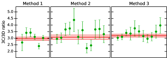
Figure S1: Experimental 3C/3D ratio for the three different methods. The individual measurements are shown as solid green circles. The weighted mean experimental values and associated 1-$\sigma$ statistical and systematic uncertainties are indicated as red band.

Table S2: $3C/3D$ oscillator strength ratios obtained from three diffferent measurement methods and their statistical and systematic uncertainties.

	Method 1	Method 2	Method 3
$3C/3D$ oscillator strength ratio	2.960	3.080	3.210
Uncertainty Budget
Statistical	0.106	0.140	0.095
Systematics due to:
(1) ROI width selection on 2D histogram (Fig. 2 of the main paper)	0.030
(2) ROI centroid selection on 2D histogram	0.044
(3) Filter transmission and efficiency of the detector	0.030	0.031	0.032
(4) Time-dependent background variation due to the electron-impact excitation	0.036
(5) Monochromator shifts in the (set) energy position		0.092
(6) Linewidth constraints in Gaussian fits			0.048
Total systematic uncertainty	0.071	0.097	0.058
Total (statistical + systematic) uncertainties	0.127	0.170	0.111
Common systematics for all three methods:
Flux variation of the incident photon beam at P04/PETRA III	0.0618
Final $3C/3D$ oscillator strength ratio	3.09 $\pm$ 0.08stat. $\pm$ 0.06sys.

I.2 Resolving Fe XVII 3D and Fe XVI C lines

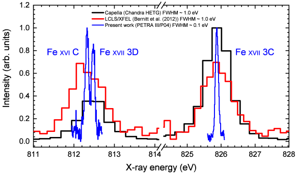
Figure S2: Spectral resolution comparison between the present work at PETRA III/P04, our previous work at LCLS/XFEL Bernitt et al. (2012), and the high resolution Chandra High Energy Transmission Grating (HETG) Canizares et al. (2000) spectrum of Capella [ObsId: 1103]. In this work, for the first time, we have resolved previously-blended Fe xvi C from Fe xvii 3D line, which are 154.3(1.3) meV apart from each other. This enables us to obtain the line intensity ratio of Fe xvii 3C and 3D without having to subtract the contribution of the Fe xvi C line, in contrast to all other previous works. Moreover, this has largely reduced the systematic uncertainties and eliminated the need for taking resonance-induced population transfer Wu and Gao (2019) into account, which may have affected the accuracy of our LCLS work Bernitt et al. (2012).

I.3 Comparison between experimental data, theoretical predictions and astrophysical observations

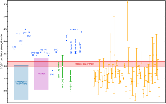
Figure S3: Present experimental 3C/3D ratios – combined results of three different methods (red band), compared with previous predictions and experiments. Blue open circles: Values from spectral databases. Blue crosses: theoretical predictions. Blue solid circles: our present FAC Shah et al. (2019); Gu (2008), large-scale CI (Sec. II.1), MR-MCDHF (Sec. II.2)), and AMBiT (Sec. II.3) calculations. Open green diamonds: previous EBIT results. Purple band: spread of Tokamak results Beiersdorfer et al. (2004). Light blue band: range of ratios observed in the Sun Blake et al. (1965); McKenzie et al. (1980), Capella Mewe et al. (2001); Behar et al. (2001), and NGC4636 Xu et al. (2002). Orange solid circles: 46 astrophysical observations of 26 stellar coronae Ness, J.-U. et al. (2003) sampled by the RGS onboard XMM-Newton and the LETGS/HETGS onboard Chandra observatories. Note that the numbers in the square bracket corresponds to the references cited in the main paper.

I.4 Estimation of photon peak intensity on sample at P04 PETRA III

For an estimation of the photon beam intensity on the plasma sample, we refer to the technical parameters of beamline P04 Viefhaus et al. (2013) and generously assume a total time-averaged photon flux after monochromatization of the beam of $\Phi_{\mathrm{Beam}}=$4\text{\times}{10}^{12}\text{\,}\mathrm{p}\mathrm{h}\mathrm{o}\mathrm{t}\mathrm{o}\mathrm{n}\mathrm{s}\mathrm{/}\mathrm{s}$,$ a focal spot size of $1\text{\times}{10}^{-6}\text{\,}{\mathrm{cm}}^{2}$, and a photon energy of $825\text{\,}\mathrm{eV}$. The $16\text{\,}\mathrm{ns}$ pulse separation ensures that the upper state population has sufficient time to completely relax into the ground state in between the pulses. We obtain a total energy per bunch of

$$E_{\mathrm{bunch}}\approx$8.5\text{\times}{10}^{-6}\text{\,}\mathrm{J}\text{\,}{\mathrm{cm}}^{-2}$.$$ (S1)

Combined with the typical pulse duration of $44\text{\,}\mathrm{ps}$ given by the official PETRA III datasheet (see  and ), we deduce an average intensity per pulse of

$$I\approx$1.9\text{\times}{10}^{5}\text{\,}\mathrm{W}\text{\,}{\mathrm{cm}}^{-2}$.$$ (S2)

For typical pulse shapes, the peak intensity can be expected to be well below $1\text{\times}{10}^{6}\text{\,}\mathrm{W}\text{\,}{\mathrm{cm}}^{-2}$.

II Calculations of 3C and 3D Oscillator Strengths

II.1 Very large-scale CI calculations

We start from the solution of the Dirac-Hartree-Fock equations in the central field approximation to construct the one-particle orbitals. The calculations are carried out using a configuration interaction (CI) method, correlating all 10 electrons. The Breit interaction is included in all calculations. The QED effects are included following Ref. Tupitsyn et al. (2016). The basis sets of increasing sizes are used to check for convergence of the values. The basis set is designated by the highest principal quantum number for each partial wave included. For example, $[5spdf6g]$ means that all orbitals up to $n=5$ are included for the $spdf$ partial waves and $n=5,6$ orbitals are included for the $g$ partial waves. We find that the inclusion of the $6,7h$ orbitals does not modify the results of the calculations and omit higher partial waves. The CI many-electron wave function is obtained as a linear combination of all distinct states of a given angular momentum $J$ and parity Dzuba et al. (1996):

$$\Psi_{J}=\sum_{i}c_{i}\Phi_{i}\,.$$ (S3)

The energies and wave functions are determined from the time-independent multiparticle Schrödinger equation $H\Phi_{n}=E_{n}\Phi_{n}.$

Table S3: Contributions to the energies of Fe¹⁶⁺ calculated with increased size basis sets and a number of configurations. The results are compared with experiment. All energies are given in cm^-1 with exception of the last line that shows the difference of the 3C and 3D energies in eV. The basis set is designated by the highest quantum number for each partial wave included. For example, $12spdfg$ means that all orbitals up to $n=12$ are included for $spdfg$ partial waves. Contributions from triple excitations, excitations from the $1s^{2}$ shells, and QED contributions are given separately.

Configuration		Expt. Kramida et al. (2018)	Expt. S_A	$[5spdf6g]$	Triples	$1s^{2}$	$+[12spdfg]$	$+[17dfg]$	QED	Final	Diff. Kramida et al. (2018)	Diff. S_A	Diff. S_A
$2p^{6}$	${}^{1}S_{0}$	0	0	0	0	0	0	0	0	0	0	0
$2p^{5}3p$	${}^{3}S_{1}$	6093450	6093295	6087185	6	254	3876	772	67	6092159	1291	1136	0.02%
$2p^{5}3p$	${}^{3}D_{2}$	6121690	6121484	6116210	-21	24	2886	701	43	6119842	1848	1642	0.03%
$2p^{5}3p$	${}^{3}D_{3}$	6134730	6134539	6129041	-23	25	3015	711	94	6132864	1866	1675	0.03%
$2p^{5}3p$	${}^{1}P_{1}$	6143850	6143639	6138383	-11	41	2825	704	82	6142025	1825	1614	0.03%
$2p^{5}3s$	$2$	5849490	5849216	5842248	-10	108	3408	735	787	5847276	2214	1940	0.03%
$2p^{5}3s$	$1$	5864770	5864502	5857770	-10	70	3303	708	784	5862626	2144	1876	0.03%
$2p^{5}3s$	$1$	5960870	5960742	5953697	-10	74	3364	717	1042	5958883	1987	1859	0.03%
$2p^{5}3d$	${}^{3}P_{1}$	6471800	6471640	6466575	-11	16	2384	665	87	6469717	2083	1923	0.03%
$2p^{5}3d$	${}^{3}P_{2}$	6486400	6486183	6481385	-13	16	2250	658	86	6484383	2017	1800	0.03%
$2p^{5}3d$	${}^{3}F_{4}$	6486830	6486720	6482549	-12	27	1745	622	97	6485028	1802	1692	0.03%
$2p^{5}3d$	${}^{3}F_{3}$	6493030	6492651	6488573	-14	26	1740	607	84	6491016	2014	1635	0.03%
$2p^{5}3d$	${}^{1}D_{2}$	6506700	6506537	6502481	-17	21	1696	627	88	6504895	1805	1642	0.03%
$2p^{5}3d$	${}^{3}D_{3}$	6515350	6515203	6511163	-18	18	1762	604	87	6513617	1733	1586	0.02%
$2p^{5}3d$	${}^{3}D_{1}$	6552200	6552503	6548550	-16	-3	1747	616	134	6551029	1171	1474	0.02%
$2p^{5}3d$	${}^{3}F_{2}$	6594360	6594309	6589977	-16	22	1729	629	335	6592676	1684	1633	0.02%
$2p^{5}3d$	${}^{3}D_{2}$	6600950	6600998	6596316	-17	14	1947	641	334	6599235	1715	1763	0.03%
$2p^{5}3d$	${}^{1}F_{3}$	6605150	6605185	6600744	-17	19	1803	610	343	6603501	1649	1684	0.03%
$2p^{5}3d$	${}^{1}P_{1}$	6660000	6660770	6656872	-8	-52	1743	619	288	6659462	538	1308	0.02%
3C-3D		13.3655	13.4234	13.4302	0.0009	-0.0061	-0.0005	0.0004	0.0191	13.4440	-0.0785	-0.0206	0.15%

We start with all possible single and double excitations to any orbital up to $5spdf6g$ from the $2s^{2}2p^{6}$, $2s^{2}2p^{5}3p$ even and $2s^{2}2p^{5}3s$, $2s^{2}2p^{5}3d$, $2s2p^{6}3p$, $2s^{2}2p^{5}4d$, $2s^{2}2p^{5}5d$ odd configurations, correlating 8 electrons. We verified that inclusion of the $2s2p^{6}3s$, $2s^{2}2p^{5}4f$, $2s^{2}2p^{5}5f$ even and $2s2p^{6}4p$, $2s^{2}2p^{5}4s$, and $2s^{2}2p^{5}5s$ odd configurations as basic configurations have negligible effect on either energies of relevant matrix elements.

The only unusually significant change in the ratio, by 0.07, is due to the inclusion of the $2s^{2}2p^{3}3d^{3}$ and $2p^{5}3d^{3}$ configurations. These are obtained as double excitations from the $2s^{2}2p^{5}3d$ odd configuration, prompting the inclusion of the $2s^{2}2p^{5}4d$, $2s^{2}2p^{5}5d$ to the list of the basic configurations.

Contributions to the energies of Fe¹⁶⁺ calculated with different size basis sets and a number of configurations are listed in Table S3. The results are compared with experimental data from the NIST database Kramida et al. (2018) and from a revised analysis of the experimental data S_A . We use LS coupling and NIST data term designations for comparison purposes, but note that $jj$ coupling would be more appropriate for this ion. Contributions to the E1 reduced matrix elements $D(3D)=D(2p^{6}$ ${}^{1}S_{0}-2p^{5}3d$ ${}^{3}D_{1})$ and $D(3C)=D(2p^{6}$ ${}^{1}S_{0}-2p^{5}3d$ ${}^{1}P_{1})$ and the ratio of the respective oscillator strengths

$$R=\left(\frac{D(3C)}{D(3D)}\right)^{2}\times\frac{\Delta E(3C)}{\Delta E(3D)}$$

are listed in Table S4. The energy ratio is 1.01655.

Table S4: Contributions to the $E1$ reduced matrix elements $D(3D)=D(2p^{6}$ ${}^{1}S_{0}-2p^{5}3d$ ${}^{3}D_{1})$ and $D(3C)=D(2p^{6}$ ${}^{1}S_{0}-2p^{5}3d$ ${}^{1}P_{1})$ (in a.u.) and the ratio of the respective oscillator strengths $R$. See caption of Table S3 for designations. $L$ and $V$ rows compared results obtained in length and velocity gauges for the $[12spdfg]$ basis. All other results are calculated using the length gauge. Transition rates are listed in the last row in s^-1.

		$D(3C)$	$D(3D)$	Ratio
$[5spdf6g]$		0.33492	0.17842	3.582
$[5spdf6g]$	$+$Triples	0.33493	0.17841	3.583
	Triples	0.00001	-0.00001
$[5spdf6g]$	+$1s^{2}$	0.33480	0.17849	3.577
	$1s^{2}$	-0.00012	0.00007
$[12spdfg]$	$L$	0.33527	0.17884	3.573
	$V$	0.33551	0.17894	3.574
$+[12spdfg]$		0.00036	0.00042
$+[17dfg]$		-0.00001	0.00001
QED		-0.00017	0.00030
Final		0.33498	0.17921	3.552
Recomm.				3.55(5)
Transition rate		2.238$\times 10^{13}$	6.098$\times 10^{12}$

Table S5: Contributions to the 3C and 3D line strengths $S$ and the 3C/3D oscillator strength ratios (energy ratio 1.01655 is used). Energies in eV, transition rates $A$ in s^-1 and natural linewidths $\Gamma$ in meV are listed in the last three rows of the tables.

	$S(3C)$	$S(3D)$	Ratio
Small basis	0.11217	0.03183	3.582
Medium basis	0.11241	0.03198	3.573
Large basis	0.11240	0.03199	3.572
+ triple excitations	0.11241	0.03198	3.573
+$1s^{2}$ shell excitations	0.11233	0.03201	3.567
+QED	0.11221	0.03212	3.552
Final	0.1122(2)	0.0321(4)	3.55(5)
Energies (eV)	825.67	812.22
$A$ (s-1)	$2.238(4)\times 10^{13}$	$6.10(7)\times 10^{12}$
$\Gamma$ (meV)	14.74(3)	4.02(5)

We include a very wide range of configurations obtained by triple excitations from the basic configurations as well as excitations from the $1s^{2}$ shell and find negligible corrections to both energies and matrix elements as illustrated by Tables S3 and S4. These contributions are listed as “Triples” and “$1s^{2}$” in both tables. A significant increase of the basis set from $[5spdf6g]$ to $[12spdfg]$ improves the agreement of energies with experiment but gives a very small, -0.009, contribution to the ratio. We find that the weights of the configurations containing $12fg$ orbitals are several times higher than those containing $12spd$ orbitals, so we expand the basis to include more $dfg$ orbitals. We also include $2s^{2}2p^{3}nd^{3}$ and $2p^{5}nd^{3}$ configurations up to $n=14$. The contributions to the energies of the orbitals with $n=13-17$ are $3-5$ times smaller than those with $n=6-12$, clearly showing the convergence of the values with the increase of the basis set. The effect on the ratio is negligible. The uncertainty of the NIST database energies, 3000 cm^-1 is larger than our differences with the experiment. The energies from the revised analysis of Fe¹⁶⁺ spectra  S_A are estimated to be accurate to about 90 cm^-1 and the scatter of the differences of different levels with the experiment is reduced. The last line of Table S3 shows the difference of the $3C$ and $3D$ energies in eV, with the final value 13.44(5)eV. We explored several different ways to construct the basis set orbitals. While the final results with an infinitely large basis set and complete configurations set should be identical, the convergence properties of the different basis sets vary, giving about 0.04 difference in the ratio and 0.04 eV in the $3C-3D$ energy difference at the $12spdfg$ level. Therefore, we set an uncertainty of the final value of the ratio to be $0.05$. As an independent test of the quality and completeness of the current basis set, we compare the results for $D(3C)$ and $D(3D)$ obtained in length and velocity gauges for the $[12spdfg]$ basis, see rows $L$ and $V$ in Table S4. The difference in the results is only 0.001. The final results for the line strengths $S$ and the 3C/3D oscillator strength ratio after several stages of computations are summarised in Table S5, which clearly illustrates a very small effect of all corrections.

This work was supported in part by U.S. NSF Grant No. PHY-1620687 and RFBR grants No. 17-02-00216 and No. 18-03-01220.

II.2 Multiconfiguration Dirac-Hartree-Fock calculations

In the multiconfiguration Dirac-Hartree-Fock (MCDHF) method, similarly to the CI approach outlined in the previous section, the many-electron state is given as an expansion in terms of a large set of $jj$-coupled configuration state functions [see Eq. (S3)]. In contrast to the CI calculations, in the case of MCDHF, the single-electron wave functions (orbitals) are self-consistently optimized. We use the method in one of its most recent implementations, namely, applying the GRASP2018 code package Fischer et al. (2019). For the virtual orbitals, the optimization of the orbitals was done in a layer-by-layer approach, i.e. when adding a new layer of orbitals (in our case, orbitals in the same shell) in the configuration expansions, the lower-lying single-electron functions are kept frozen.

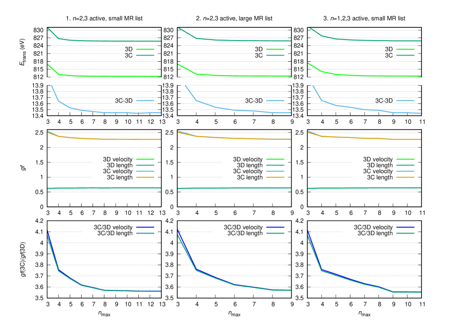
Figure S4: Convergence of the MCDHF calculations: The X-ray transition energies of the 3C and 3D lines, their difference, the weighted oscillator strengths $gf$ and their ratio vs. the maximal principal quantum number $n_{\rm max}$ used. Oscillator strengths are given both in the relativistic length (Babushkin) and velocity (Coulomb) gauges to numerically control gauge invariance. The different columns display results from different sets of calculations, as described in the text.

In a first set of calculations, we use the $2s^{2}2p^{6}$ configuration for the ground state and the $2s^{2}2p^{5}3s$, $2s^{2}2p^{5}3d$, and $2s^{1}2p^{6}3p$ $J=1$ odd configurations for the excited states to generate the configuration lists. Single and double electron exchanges from the $n=2,3$ spectroscopic (occupied) orbitals were taken into account up to virtual orbitals $n_{\rm max}spdfg$, where the maximal principal quantum number $n_{\rm max}$ is varied in the computations to study the convergence of the results. Such an approach is helpful in estimating the final theoretical uncertainty. Test calculations also using virtual orbitals with $h$ and $i$ symmetry have shown that these high angular momenta do not play a noticeable role. The ground and excited states were treated separately, i.e. two independently optimized sets of orbitals were used. After these multireference MCDHF calculations, the possible effects of further higher-order electron exchanges were included in a subsequent step, when a CI calculation was performed with the extended configuration lists (triple excitations from the multireference states up to $n=4$ orbitals, yielding approx. 800 thousand configurations for $n_{\rm max}=13$), employing the radial wave functions obtained from the previous MCDHF calculations. Furthermore, the effects of the frequency-independent Breit relativistic electron interaction operator, the normal and specific mass shift, and approximate radiative corrections are accounted for (see Fischer et al. (2019) and references therein). The QED effects have been included in the calculation of transition energies (which also enter the oscillator strengths), however, not in the electric dipole matrix elements, as such corrections are anticipated to be on the 1% level and thus can be neglected. The oscillator strengths were evaluated with the biorthogonal basis sets, each optimized separately for the ground- and excited states, to include orbital relaxation effects. The results of these calculations are presented in the first column of Fig. S4. The bottom panel shows that the oscillator strength ratio is converged from $n_{\rm max}=9$ on.

In a subsequent set of calculations, the multireference set describing the ground and excited levels were expanded to include all $J=0$ even and $J=1$ odd states with 1 or 2 electrons in the M shell. The maximal principal quantum number of the virtual orbitals was set to 9 to limit the computational expense of calculations. Results are shown in the 2nd column of Fig. S4. In a third setting, calculations were performed with the smaller multireference list as described in the previous paragraph, however, with all spectroscopic orbitals (those with $n=1,2,3$) included in the active set of orbitals when generating the configuration list. With the triple electron exchanges also included, this procedure yielded approx. 1.2 million configurations in the description of the excited states. The energies and strengths are shown in the last column of the figure. The converged 3C/3D oscillator strength ratios agree well for all 3 calculations. Comparing the different results, the final value for the ratio is 3.55(5), which agrees well with earlier large-scale MCDHF results Bernitt et al. (2012); Jönsson et al. (2014), and also with the results of the other theoretical methods described in this Supplement. For the difference of the energies of the 3C and 3D lines – which can be more accurately determined in the experiment than the absolute X-ray transition energies – we obtain 13.44(5) eV.

II.3 AMBiT: particle-hole CI method calculations

A separate CI calculation of the 3C and 3D lines in Fe¹⁶⁺ has been performed with the AMBiT code Kahl and Berengut (2019). Our calculation begins with a Dirac-Hartree-Fock calculation of Ne-like Fe to construct the core $1s$, $2s$, and $2p$ orbitals in the $V^{N}$ potential. The Breit interaction is included throughout the calculation. We diagonalize a set of $B$-splines in the Dirac-Fock potential to obtain valence orbitals. Configuration interaction is performed using the particle-hole CI method Berengut (2016), however, this can be mapped exactly to the electron-only approach described in Section II.1.

Our basic calculation is presented on the first line of Table S6. The CI space consists of all possible single and double excitations up to $10spdf$ from the same set of leading configurations presented previously: $2s^{2}\ 2p^{6}$, $2p^{-1}\ 3p$, $2p^{-1}\ 3s$, $2p^{-1}\ 3d$, $2p^{-1}\ 4d$, $2p^{-1}\ 5d$, and $2s^{-1}3p$. At this stage, we do not include excitations from the frozen $1s^{2}$ core. Even for this calculation, the matrix size for the odd-parity $J=1$ levels is $N=479\,075$. To reduce the number of stored matrix elements we use emu CI Geddes et al. (2018), where interactions between high-lying configuration state functions are ignored. We limit the smaller side of the matrix to only including double excitations up to $5spdf$ and limit the number of $2s$ and $2p$ holes to single removals from an expanded set of leading configurations which include, in addition to those listed above, $2p^{-2}\ 3d^{2}$, $2p^{-1}\ 2s^{-1}\ 3d^{2}$, and $2s^{-2}\ 3d^{2}$. This results in a reduced small side $N_{small}=80497$. We have checked that expanding the configuration state functions included in $N_{small}$ makes no difference to our results at the displayed accuracy.

All of our calculations include the Breit interaction at all stages, and the dipole matrix elements are calculated in the relativistic formulation with $\omega=30$ a.u. In the second and third lines of Table S6, we show the effects of removing the Breit interaction and using the static dipole matrix element ($\omega=0$), respectively.

We then expand our calculation to include $g$-wave excitations, up to basis $10spdfg$. The difference from $10spdf$ is shown in the fourth line of Table S6. We see in the AMBiT calculation very little effect from the inclusion of these waves. In the fifth line, we show the effect of allowing excitations from $1s^{2}$, and in the sixth line we see the effect of including the Uehling potential Ginges and Berengut (2016a) and self-energy Ginges and Berengut (2016b) using the radiative-potential method Flambaum and Ginges (2005). This broadly agrees with the model-operator QED presented in Table S4.

The final row of Table S6 gives the results including excitations to $g$-waves, excitations from $1s^{2}$, and QED effects. The total number of configuration state functions accounted for is over 1.25 million for the odd-parity $J=1$ symmetry. Nevertheless, the CI is not quite converged with respect to including orbitals with $n>10$. We estimate based on calculations for $8spdf$ and $12spdf$ that the uncertainty in level energies is conservatively of order $3000~{}\textrm{cm}^{-1}$ and for the ratio $gf_{3C}/gf_{3D}$ is of order 0.05. These results are consistent with the CI calculation presented in Sec. II.1 and the MCDHF results presented in Sec. II.2.

Table S6: Particle-hole CI calculations using AMBiT of the level energies $E_{3C}$ and $E_{3D}$ (cm^-1), reduced matrix elements $D(3C)$ and $D(3D)$ (a.u.), and ratio of oscillator strengths of the $3C$ and $3D$ transitions in Fe¹⁶⁺.

	$E_{3C}$	$E_{3D}$	$D(3C)$	$D(3D)$	$gf_{3C}/gf_{3D}$
[$10spdf$]	6661400	6552424	0.33893	0.17992	3.607
without Breit	6668847	6557636	0.33758	0.18164	3.511
$\omega=0$			0.33937	0.18009	3.610
+[$10g$]	-15	-13	-0.000001	0.000003
+$1s^{2}$	-103	-85	-0.000040	0.000016
+QED	235	94	-0.00012	0.00031
Final	6661517	6552420	0.33877	0.18025	3.591

References

- Bernitt et al. (2012) S. Bernitt, G. V. Brown, J. K. Rudolph, R. Steinbrugge, A. Graf, M. Leutenegger, S. W. Epp, S. Eberle, K. Kubicek, V. Mackel, et al., Nature 492, 225 (2012).
- Canizares et al. (2000) C. R. Canizares, D. P. Huenemoerder, D. S. Davis, D. Dewey, K. A. Flanagan, J. Houck, T. H. Markert, H. L. Marshall, M. L. Schattenburg, N. S. Schulz, et al., Astrophys. J. Lett. 539, L41 (2000).
- Wu and Gao (2019) C. Wu and X. Gao, Sci. Rep 9, 7463 (2019).
- Shah et al. (2019) C. Shah, J. R. C. López-Urrutia, M. F. Gu, T. Pfeifer, J. Marques, F. Grilo, J. P. Santos, and P. Amaro, Astrophys. J. 881, 100 (2019).
- Gu (2008) M. F. Gu, Can. J. Phys. 86, 675 (2008).
- Beiersdorfer et al. (2004) P. Beiersdorfer, M. Bitter, S. Von Goeler, and K. Hill, Astrophys. J. 610, 616 (2004).
- Blake et al. (1965) R. Blake, T. Chubb, H. Friedman, and A. Unzicker, Astrophys. J. 142, 1 (1965).
- McKenzie et al. (1980) D. L. McKenzie, P. B. Landecker, R. M. Broussard, H. R. Rugge, R. M. Young, U. Feldman, and G. A. Doschek, Astrophys. J. 241, 409 (1980).
- Mewe et al. (2001) R. Mewe, A. J. J. Raassen, J. J. Drake, J. S. Kaastra, R. L. J. van der Meer, and D. Porquet, Astron. Astrophys 368, 888 (2001).
- Behar et al. (2001) E. Behar, J. Cottam, and S. M. Kahn, Astrophys. J. 548, 966 (2001).
- Xu et al. (2002) H. Xu, S. M. Kahn, J. R. Peterson, E. Behar, F. B. S. Paerels, R. F. Mushotzky, J. G. Jernigan, A. C. Brinkman, and K. Makishima, Astrophys. J. 579, 600 (2002).
- Ness, J.-U. et al. (2003) Ness, J.-U., Schmitt, J. H. M. M., Audard, M., Güdel, M., and Mewe, R., A&A 407, 347 (2003).
- Viefhaus et al. (2013) J. Viefhaus, F. Scholz, S. Deinert, L. Glaser, M. Ilchen, J. Seltmann, P. Walter, and F. Siewert, Nucl. Instrum. Methods Phys. Res., Sect. A 710, 151 (2013).
- Note (1) https://photon-science.desy.de/facilities/petra_iii/beamlines/p04_xuv_beamline/unified_data_sheet_p04/index_eng.html.
- Note (2) https://photon-science.desy.de/facilities/petra_iii/beamlines/p04_xuv_beamline/beamline_parameters/index_eng.html.
- Tupitsyn et al. (2016) I. I. Tupitsyn, M. G. Kozlov, M. S. Safronova, V. M. Shabaev, and V. A. Dzuba, Phys. Rev. Lett. 117, 253001 (2016).
- Dzuba et al. (1996) V. A. Dzuba, V. V. Flambaum, and M. G. Kozlov, Phys. Rev. A 54, 3948 (1996).
- Kramida et al. (2018) A. Kramida, Yu. Ralchenko, J. Reader, and and NIST ASD Team, NIST Atomic Spectra Database (ver. 5.6.1), [Online]. Available: https://physics.nist.gov/asd [2019, September 6]. National Institute of Standards and Technology, Gaithersburg, MD. (2018).
- (19) A. Kramida, Preliminary critical analysis of Fe XVII spectral data, Private Communication (2019).
- Fischer et al. (2019) C. F. Fischer, G. Gaigalas, P. Jönsson, and J. Bieroń, Comput. Phys. Commun. 237, 184 (2019).
- Jönsson et al. (2014) P. Jönsson, P. Bengtsson, J. Ekman, S. Gustafsson, L. Karlsson, G. Gaigalas, C. F. Fischer, D. Kato, I. Murakami, H. Sakaue, et al., At. Data Nucl. Data Tables 100, 1 (2014).
- Kahl and Berengut (2019) E. V. Kahl and J. C. Berengut, Comput. Phys. Commun 238, 232 (2019).
- Berengut (2016) J. C. Berengut, Phys. Rev. A 94, 012502 (2016).
- Geddes et al. (2018) A. J. Geddes, D. A. Czapski, E. V. Kahl, and J. C. Berengut, Phys. Rev. A 98, 042508 (2018).
- Ginges and Berengut (2016a) J. S. M. Ginges and J. C. Berengut, J. Phys. B: At., Mol. Opt. Phys. 49, 095001 (2016a).
- Ginges and Berengut (2016b) J. S. M. Ginges and J. C. Berengut, Phys. Rev. A 93, 052509 (2016b).
- Flambaum and Ginges (2005) V. V. Flambaum and J. S. M. Ginges, Phys. Rev. A 72, 052115 (2005).