The Unusual Broadband X-ray Spectral Variability of NGC 1313 X-1 seen with XMM-Newton, Chandra and NuSTAR

Abstract

We present results from the major coordinated X-ray observing program on the ULX NGC 1313 X-1 performed in 2017, combining XMM-Newton, Chandra and NuSTAR, focusing on the evolution of the broadband ($\sim$0.3–30.0 keV) continuum emission. Clear and unusual spectral variability is observed, but this is markedly suppressed above $\sim$10–15 keV, qualitatively similar to the ULX Holmberg IX X-1. We model the multi-epoch data with two-component accretion disc models designed to approximate super-Eddington accretion, allowing for both a black hole and a neutron star accretor. With regards to the hotter disc component, the data trace out two distinct tracks in the luminosity–temperature plane, with larger emitting radii and lower temperatures seen at higher observed fluxes. Despite this apparent anti-correlation, each of these tracks individually shows a positive luminosity–temperature relation. Both are broadly consistent with $L\propto{T}^{4}$, as expected for blackbody emission with a constant area, and also with $L\propto{T}^{2}$, as may be expected for an advection-dominated disc around a black hole. We consider a variety of possibilities for this unusual behaviour. Scenarios in which the innermost flow is suddenly blocked from view by outer regions of the super-Eddington disc/wind can explain the luminosity–temperature behaviour, but are difficult to reconcile with the lack of strong variability at higher energies, assuming this emission arises from the most compact regions. Instead, we may be seeing evidence for further radial stratification of the accretion flow than is included in the simple models considered, with a combination of winds and advection resulting in the suppressed high-energy variability.

1 Introduction

NGC 1313 X-1 is one of the archetypal ultraluminous X-ray sources (ULXs). These are off-nuclear X-ray sources that appear to radiate in excess of $10^{39}$ erg s^-1, roughly the Eddington limit for the stellar remnant black holes ($M_{\rm{BH}}\sim 10$ $\rm M_{\odot}$) that power X-ray binaries in our own Galaxy (see Kaaret et al. 2017 for a recent review). Although they were historically considered good candidates for hosting intermediate mass black holes (IMBHs, $M_{\rm{BH}}\sim 10^{2-5}$ $\rm M_{\odot}$; e.g. Miller et al. 2003, 2004; Miller & Colbert 2004; Strohmayer & Mushotzky 2009), the broadband X-ray spectra observed in the NuSTAR era show clear deviations from the standard sub-Eddington accretion modes which would be expected for such objects (e.g. Bachetti et al. 2013; Walton et al. 2013, 2014, 2015a, 2015b, 2017; Sazonov et al. 2014; Rana et al. 2015; Mukherjee et al. 2015; Annuar et al. 2015; Luangtip et al. 2016; Krivonos & Sazonov 2016; Fürst et al. 2017; Shidatsu et al. 2017). These observations confirmed the previous indications for these deviations seen in the more limited XMM-Newton bandpass (Stobbart et al. 2006; Gladstone et al. 2009), and imply instead that the majority of ULXs likely represent a population of X-ray binaries accreting at high/super-Eddington rates.

This conclusion was further cemented with the remarkable discovery that a number of ULXs are actually powered by accreting pulsars (Bachetti et al. 2014; Fürst et al. 2016; Israel et al. 2017a, b; Carpano et al. 2018; Sathyaprakash et al. 2019; Rodríguez Castillo et al. 2019). These sources therefore appear to exceed their Eddington limits by factors of up to $\sim$500, and their broadband spectra are qualitatively similar to the rest of the ULX population, particularly at high energies ($E>10$ keV; Pintore et al. 2017; Koliopanos et al. 2017; Walton et al. 2018b, c). Two other ULXs in M51 have also been identified as likely hosting neutron star accretors via other means, first through the detection of a potential cyclotron resonant scattering feature (Brightman et al. 2018), and second through the detection of a potentially bi-modal flux distribution (as expected for a source transitioning to and from the propeller regime; Earnshaw et al. 2018). A number of other candidates for such transitions have also recently been reported among the broader ULX population (Song et al. 2020). Although the known ULX pulsars are now firmly established as being powered by magnetised neutron stars, the strength of the magnetic fields in these systems is still the subject of significant debate, with estimates ranging from $\sim$10^9-15 G and some models invoking higher-order field geometries (e.g. quadrupolar) than the standard dipole fields typically assumed (e.g. Bachetti et al. 2014; Dall’Osso et al. 2015; Mushtukov et al. 2015; Kluźniak & Lasota 2015; Fürst et al. 2016; Brightman et al. 2018; Walton et al. 2018a; Vasilopoulos et al. 2018; Middleton et al. 2019).

One of the fundamental predictions of super-Eddington accretion is that strong winds are launched from the accretion flow, as radiation pressure exceeds gravity (e.g. Shakura & Sunyaev 1973; Poutanen et al. 2007; Dotan & Shaviv 2011; Takeuchi et al. 2013). Observational evidence for such winds in ULXs was only recently seen for the first time in NGC 1313 X-1, through the detection of strongly blueshifted atomic features (Pinto et al. 2016; Walton et al. 2016a; see also Middleton et al. 2015b), and such features have now been seen in several other systems (including NGC 300 ULX1, one of the known pulsars; Pinto et al. 2017; Kosec et al. 2018a, b). These winds are extreme, reaching velocities of up to $\sim$0.25$c$, and, despite the extreme X-ray luminosities of these sources, may actually dominate their total energetic output.

In order to study the variability of the extreme outflow in NGC 1313 X-1, we performed a series of coordinated broadband X-ray observations of the NGC 1313 galaxy combining data from XMM-Newton (PI: Pinto), Chandra (PI: Canizares) and NuSTAR (PI: Walton). This program has already provided a variety of interesting results, revealing clear variability in the wind in X-1 (Pinto et al. 2020), a $\sim$150 s soft X-ray lag in X-1 (Kara et al. 2020), and the detection of pulsations in X-2 (Sathyaprakash et al. 2019). Here we combine these observations with the coordinated XMM-Newton and NuSTAR observations available in the archive to study the broadband continuum variability exhibited by NGC 1313 X-1.

Table 1: Details of the X-ray observations of NGC 1313 used in this work.

Epoch	Mission(s)	OBSID(s)	Start	Exposure[a]
			Date	(ks)
XN1	NuSTAR	30002035002	2012-12-16	154
	NuSTAR	30002035004	2012-12-21	206
	XMM-Newton	0693850501	2012-12-16	85/112
	XMM-Newton	0693851201	2012-12-22	79/120
XN2	NuSTAR	80001032002	2014-07-05	73
	XMM-Newton	0742590301	2014-07-05	54/61
XN3	NuSTAR	90201050002	2017-03-29	125
	XMM-Newton	0794580601	2017-03-29	25/38
XN4	NuSTAR	30302016002	2017-06-14	100
	XMM-Newton	0803990101	2017-06-14	110/130
	XMM-Newton	0803990201	2017-06-20	111/129
CN1	NuSTAR	30302016004	2017-07-17	87
	Chandra	19929	2017-07-03	18
	Chandra	20105	2017-07-06	31
	Chandra	19712	2017-07-18	49
	Chandra	20125	2017-08-01	25
	Chandra	20126	2017-08-02	27
	Chandra	19714	2017-08-03	20
	Chandra	19927	2017-08-05	25
XN5	NuSTAR	30302016006	2017-09-03	90
	XMM-Newton	0803990301	2017-08-31	45/101
	XMM-Newton	0803990401	2017-09-02	83/81
CN2	NuSTAR	30302016008	2017-09-15	108
	Chandra	19928	2017-08-28	21
	Chandra	20729	2017-09-16	10
	Chandra	20637	2017-09-24	28
	Chandra	19713	2017-09-26	32
	Chandra	20798	2017-09-29	17
XN6[b]	NuSTAR	30302016010	2017-12-09	100
	XMM-Newton	0803990601	2017-12-09	69/115

^a Good exposures used for our spectral analysis, given to the nearest ks; XMM-Newton exposures are listed for the EPIC-pn/MOS detectors, and the NuSTAR exposures combine both modes 1 and 6 (see Section 2.1).
^b Although two XMM-Newton observations were taken as part of epoch XN6, the two show markedly different spectra, so we only make use of the XMM-Newton observation taken simultaneously with the NuSTAR exposure for this epoch (see Section 3.1).

Figure 1: The long-term 0.3–10 keV X-ray lightcurve seen by Swift XRT since October 2012. The timing of the NuSTAR observations, which define the broad epochs considered here, are indicated by the red dashed lines for coordination with XMM-Newton, and blue dashed lines for coordination with Chandra. The period after MJD $\sim$ 57400 shows enhanced variability, which is covered by a number of our broadband observations.

2 Observations and Data Reduction

During the main 2017 campaign, XMM-Newton (Jansen et al. 2001) observed NGC 1313 with its full suite of instrumentation for six full orbits ($\sim$750 ks total exposure), grouped into three pairs of observations, with the two observations constituting each pair taken in relatively quick succession. Chandra (Weisskopf et al. 2002) also performed a series of observations across 2017, totalling $\sim$500 ks exposure. Although these Chandra observations are relatively well spread across the year, there are two periods where a number of the observations are clustered in time. In addition to these soft X-ray observations, NuSTAR (Harrison et al. 2013) also performed a series of five exposures over the second half of 2017 ($\sim$500 ks total exposure). One was performed with each of the pairs of XMM-Newton observations, taken simultaneously with one of the two exposures, and the remaining two were taken with the two main clusters of Chandra observations, again performed simultaneously with one of the exposures in these two groups.

In addition to these observations, XMM-Newton and NuSTAR have also performed coordinated observations on a few prior occasions. There were two deep observations taken in quick succession soon after the launch of NuSTAR in 2012 (see Bachetti et al. 2013; Miller et al. 2014; Walton et al. 2016a), as well as shorter coordinated observations taken in 2014 and again in 2017 prior to the commencement of the main campaign. Details of the observations considered in this work are given in Table 1, and the following sections describe our data reduction procedure for the various missions involved.

2.1 NuSTAR

We reduced the NuSTAR data as standard with the NuSTAR Data Analysis Software (v1.8.0; part of the HEASOFT distribution) and NuSTAR caldb v20171204. The unfiltered event files were cleaned with NUPIPELINE. We used the standard depth correction, which significantly reduces the internal background at high energies, and periods of earth-occultation and passages through the South Atlantic Anomaly were also excluded. To be conservative, source products were extracted from circular regions of radius 30^′′, owing to the presence of another faint source to the south (see Bachetti et al. 2013), and the background was estimated from a larger, blank area on the same detector, free of contaminating point sources (the exact size of the background region used varies between epochs, depending on the position angle of the observation and the proximity of the source to the edge of the detector). Spectra and lightcurves were extracted from the cleaned event files using NUPRODUCTS for both focal plane modules (FPMA and FPMB). In addition to the standard ‘science’ data (mode 1), we also extract the ‘spacecraft science’ data (mode 6) following Walton et al. (2016b). This provides $\sim$20–40% of the total good exposure, depending on the specific observation.

2.2 XMM-Newton

For the XMM-Newton observations, data reduction was carried out with the XMM-Newton Science Analysis System (SAS v16.1.0). Here we focus on the data taken by the EPIC CCD detectors – EPIC-pn and EPIC-MOS (Strüder et al. 2001; Turner et al. 2001) – for our continuum analysis; the high-resolution data from the RGS (den Herder et al. 2001) will be presented in a separate work (Pinto et al. 2020). The raw observation data files were processed as standard using EPCHAIN and EMCHAIN. Source products were extracted from circular regions of radius $\sim$30^′′, and, as before, the background was estimated from larger areas on the same CCD free from contaminating point sources (again, the exact size of the background region used varies from epoch to epoch, depending on the position angle of the observation and, for the EPIC-pn detector, the position of the read-out streak relative to other nearby sources). Lightcurves and spectra were generated with XMMSELECT, excluding periods of high background and selecting only single and double events for EPIC-pn (PATTERN$\leq$4), and single to quadruple events for EPIC-MOS (PATTERN$\leq$12). The redistribution matrices and auxiliary response files for each detector were generated with RMFGEN and ARFGEN, respectively. After performing the data reduction separately for each of the MOS detectors, and confirming their consistency, these spectra were combined using the FTOOL ADDASCASPEC for each OBSID. Finally, where spectra from different OBSIDs were merged, these were also combined using ADDASCASPEC.

2.3 Chandra

High spectral resolution X-ray spectroscopy is provided by the Chandra-High Energy Gratings Spectrometer (HETGS Canizares et al., 2005), which consists of two gratings sets: the Medium Energy Gratings (MEG, $E/\Delta E\approx 700$ at 1 keV) and the High Energy Gratings (HEG, $E/\Delta E\approx 1300$ at 1 keV). Each gratings set, MEG and HEG, disperses spectra into negative and positive orders. Throughout this work, as we describe below, we combine the $\pm 1^{\rm st}$ order spectra into a single spectrum for each gratings instrument (appreciable counts in the higher orders are only obtained for very bright sources, so are ignored in our analyses). The HETG also produces an undispersed $\mathrm{0^{th}}$ order spectrum, but it suffers from photon pileup (Davis, 2001), so we do not consider it further.

The Chandra-HETG spectra were created using the Interactive Spectral Interpretation System (ISIS; Houck & Denicola 2000) running extraction scripts from the Transmission Gratings Catalogue (TGcat; Huenemoerder et al., 2011). These scripts in turn ran tools from CIAO v4.10 and utilized Chandra caldb v4.7.8. The position of the $0^{\rm th}$ order image was determined by the TGDETECT tool, which then defined the identification and extraction regions for the $\pm 1^{\rm st}$ orders of the MEG and HEG. Specifically, events within an 18 pixel radius of the $0^{\rm th}$ order image were assigned to $0^{\rm th}$ order, while any events that fell within $\pm 18$ pixels of the cross dispersion direction of either the MEG or HEG spectra were assigned to that grating arm using the TG_CREATE_MASK tool. In overlap regions, events are preferentially assigned to $0^{\rm th}$, MEG, and then HEG, respectively. Within these identification regions, events that were within $\pm 1^{\prime\prime}$ of the HEG and MEG dispersion arm locations were extracted (TG_EXTRACT) and assigned to a given spectral order with TG_RESOLVE_EVENTS using the default settings, while background spectra were extracted from regions that lay 3–8.5^′′ perpendicularly from the dispersion arm locations. The standard tools, FULLGARF and MKGRMF, were used to create the spectral response matrices. Finally, for a given set of gratings (HEG or MEG) the spectra were combined for $\pm 1^{\rm st}$ orders using ADDASCASPEC for each OBSID, and where spectra from multiple OBSIDs were combined we again used ADDASCASPEC.

3 Spectral Analysis

Our focus on this work is on broadband spectroscopy of NGC 1313 X-1. All of the datasets analysed are rebinned to have a signal-to-noise (S/N) ratio of at least 5 per energy bin, using a combination of SPECGROUP in the XMM-Newton SAS  and custom software, and we fit the data using $\chi^{2}$ minimisation. The XMM-Newton EPIC datasets are analysed over the 0.3–10.0 keV range, the Chandra MEG and HEG gratings data over the 0.6–6.0 and 0.8–8.0 keV ranges, respectively, and the NuSTAR FPMA/B data provide coverage up to $\sim$25–35 keV, depending on the dataset (above which the S/N drops below 5). We perform spectral analysis with XSPEC v12.10.0 (Arnaud 1996) throughout, and quote parameter uncertainties at the 90% confidence level for one interesting parameter ($\Delta\chi^{2}=2.7$). We allow multiplicative constants to float between the datasets from a given epoch to account for cross-calibration uncertainties between the different detectors, with FPMA fixed at unity as one of the detectors common to all epochs; these constants are within $\sim$10% of unity, as expected (Madsen et al. 2015). Throughout this work, we assume a distance of $D=4.2$ Mpc to NGC 1313 (Méndez et al. 2002; Tully et al. 2016).

3.1 Data Organisation

The observations considered are naturally grouped into several broad epochs, largely determined by the NuSTAR coverage; we refer to the coordinated XMM-Newton+NuSTAR epochs as XN$i$, and the coordinated Chandra+NuSTAR epochs as CN$i$, where $i$ indicates the chronology for each combination (see Table 1; note that we do not require strict simultaneity between the data from the relevant observatories when defining these epochs, and that the observations combined to form each epoch are all taken within $\sim$2 weeks of the NuSTAR exposures around which they are defined). Figure 1 shows the NuSTAR coverage in the context of the long-term behaviour from NGC 1313 X-1 seen by the Neil Gehrels Swift Observatory (hereafter Swift; Gehrels et al. 2004), extracted using the standard online pipeline (Evans et al. 2009). These epochs cover a range of fluxes, and also the period of enhanced variability seen more recently by Swift (commencing MJD $\sim$ 57400).

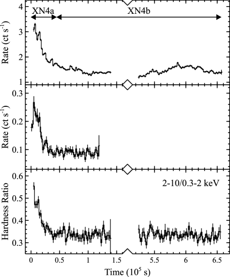
Figure 2: Lightcurves from the observations that form epoch XN4 (2 ks time bins). The top panel shows the 0.3–10.0 keV lightcurve observed with the EPIC-pn detector over the two XMM-Newton exposures, and the middle panel shows the 3–30 keV lightcurve observed with the NuSTAR FPMA detector. The bottom panel also shows a hardness ratio computed between the 0.3–2.0 and 2.0–10.0 keV bands, based on the EPIC-pn count rates. Clear spectral variability is seen towards the beginning of these observations, after which the spectrum appears to stabilize (even if some flux variability is still observed). For our spectral analysis we therefore split these data into two sub-epochs, which we refer to as XN4a and XN4b, as indicated by the horizontal arrows.

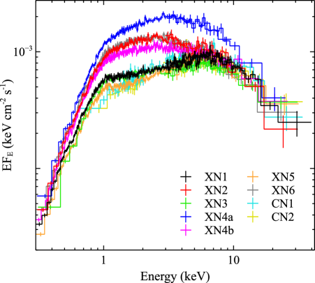
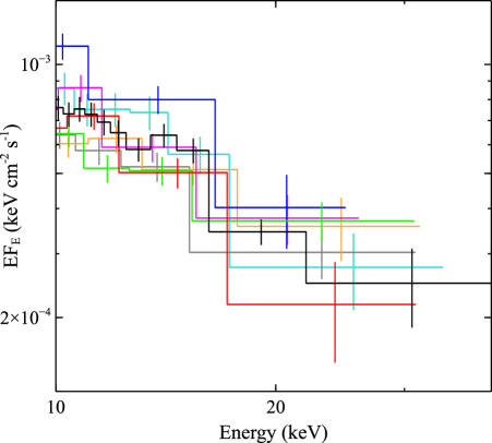
Figure 3: Left: The broadband spectral evolution displayed by NGC 1313 X-1. For clarity, we only show the EPIC-pn data for XMM-Newton and the MEG data for Chandra (where relevant), and the FPMA data for NuSTAR. Given the large number of datasets shown, we show the soft and hard X-ray coverage from each epoch in the same colour. The XMM-Newton data span the $\sim$0.3–10.0 keV range, the Chandra data shown span the $\sim$0.6–6.0 keV range, and the NuSTAR data span the $\sim$3–35 keV range. Despite the strong variations at lower energies (below $\sim$10 keV), the higher energy data (above $\sim$10 keV) are relatively stable. Right: A zoom in on the high-energy ($>$10 keV) data from NuSTAR (again, FPMA only for clarity), further demonstrating the relative lack of variability observed at these energies in comparison to the lower energy data. All the data have been unfolded through a simple model that is constant with energy, and have been further rebinned for visual purposes.

The two broadband observations performed in quick succession in 2012 are considered to be a single epoch (XN1) in this work, as they both exhibit the same spectrum and there is negligible variability within either of the observations (Bachetti et al. 2013). Epoch XN4 coincidentally caught the end of a relatively large flare (see Figure 1), with NGC 1313 X-1 showing strong flux and spectral evolution across the simultaneous XMM-Newton+NuSTAR exposure (see Figure 2). We therefore split the data from this epoch into higher and lower flux periods, which we refer to as epochs XN4a and XN4b respectively. The XN4a spectrum is extracted from the first 45 ks of the simultaneous exposure (OBSIDs 0803990101 and 30302016002; this is the point at which the high-energy ($E>3$ keV) flux/spectral variability stabilises), while the XN4b spectrum is extracted from the remaining data from these OBSIDs, combined with the second XMM-Newton exposure (OBSID 0803990201), which exhibited similar flux and spectral shape. None of the other new observations considered here show notable spectral variability within any of the individual exposures. The two XMM-Newton observations taken during epoch XN5 show consistent spectra, and so are combined. However, the two XMM-Newton observations taken during epoch XN6 do show clearly different spectra, and so in this case we only consider the XMM-Newton data from the exposure taken simultaneously with NuSTAR. We also note that, owing to the spread of the full Chandra dataset, for epochs XN5 and XN6 there are also short Chandra observations contemporaneous with the XMM-Newton and NuSTAR data, but in these cases we only consider the higher S/N XMM-Newton data for the soft X-ray coverage. For epochs CN1 and CN2, we confirmed that the spectra from each of the individual Chandra observations grouped together were consistent, before combining them further into the final merged spectra used in our analysis.

3.2 Broadband Spectral Variability

The nine broadband spectra extracted are shown in Figure 3. The spectral variability exhibited by NGC 1313 X-1 shows remarkable similarity to the behaviour seen from Holmberg IX X-1 (Walton et al. 2014, 2017; Luangtip et al. 2016), another well-studied ULX; the variability is strong at lower energies (below $\sim$10 keV), with the spectrum becoming more centrally peaked at higher fluxes, but the higher energy data (above $\sim$10 keV) appears to remain extremely similar for all of the spectra compiled to date. To illustrate this, we model the NuSTAR data above 10 keV with a simple powerlaw model. The photon indices are all consistent within their 90% confidence limits (fitting all of the datasets together we find $\Gamma=3.2\pm 0.1$), and the 10–40 keV fluxes only vary by at most a factor of $\sim$1.5, despite the factor of $>$3 differences seen at $\sim$3 keV.

As the nature of the accretor in NGC 1313 X-1 remains unknown (no pulsations have been seen from NGC 1313 X-1 to date; see Appendix A), we construct two models to fit the broadband data that may approximate super-Eddington accretion onto a non-magnetic accretor (either a black hole or an non-magnetic neutron star; note that super-Eddington accretion onto a non-magnetic neutron star is expected to be conceptually similar to the black hole case, with a standard outer disc, a funnel-like inner region and strong winds, e.g. King 2008, although for a given luminosity the accretion rate relative to Eddington would naturally be more extreme in the former) and a magnetic accretor (i.e. a ULX pulsar), respectively, although we stress that these models are still strictly phenomenological. Throughout this work, we include two neutral absorbers in all of our modelling, the first fixed to the Galactic column of $N_{\rm{H}}=4.13\times 10^{20}$ cm^-2 (Kalberla et al. 2005), and the second free to account for absorption local to NGC 1313 ($z=0.00157$). For the neutral absorption, we use the TBABS absorption model, combining the solar abundances of Wilms et al. (2000) and the cross-sections of Verner et al. (1996). We also note again that NGC 1313 X-1 is known to show atomic features in both absorption and emission, particularly at low energies (Middleton et al. 2014; Pinto et al. 2016; Walton et al. 2016a). However, here we are interested in the spectral variability of the continuum emission, and these features do not strongly influence the broadband continuum fits, so we do not treat them here; instead the atomic emission/absorption will be the subject of separate works (Pinto et al. 2020; Nowak et al., in preparation).

Table 2: Best-fit parameters from the nine broadband spectra currently available for NGC 1313 X-1 for the models assuming a non-magnetic and a magnetic accretor, respectively

Model	Parameter						Epoch
Component			XN1	XN2	XN3	XN4a	XN4b	CN1	XN5	CN2	XN6
Non-Magnetic Accretor Model: TBABS$\times$ $($ DISKBB $+$ DISKPBB $\otimes$ SIMPL $)$
TBABS	$N_{\rm{H,int}}$[a]	[$10^{21}$ cm-2]	$2.47^{+0.05}_{-0.08}$	–	–	–	–	–	–	–	–
DISKBB	$T_{\rm{in}}$	[keV]	$0.27\pm 0.01$	$0.35^{+0.03}_{-0.02}$	$0.30\pm 0.01$	$0.36\pm 0.02$	$0.33\pm 0.01$	$0.16^{+0.07}_{-0.05}$	$0.25\pm 0.01$	$0.18^{+0.07}_{-0.06}$	$0.32\pm 0.01$
	Norm		$17.3^{+2.0}_{-2.3}$	$4.5^{+2.1}_{-1.6}$	$9.9^{+1.6}_{-1.4}$	$7.2^{+1.9}_{-2.1}$	$6.7^{+1.2}_{-1.0}$	$160^{+2930}_{-140}$	$21.8^{+2.7}_{-3.1}$	$67^{+728}_{-58}$	$8.9^{+2.7}_{-2.2}$
DISKPBB	$T_{\rm{in}}$	[keV]	$3.0^{+0.2}_{-0.3}$	$1.0^{+0.3}_{-0.1}$	$1.9^{+0.9}_{-0.5}$	$1.6^{+0.1}_{-0.2}$	$1.3^{+0.2}_{-0.1}$	$3.1\pm 0.7$	$2.3\pm 0.4$	$2.9^{+0.8}_{-1.0}$	$0.9^{+0.2}_{-0.1}$
	$p$		$0.58\pm 0.01$	$0.55^{+0.03}_{-0.01}$	$0.59^{+0.04}_{-0.02}$	$0.61^{+0.05}_{-0.03}$	$0.55^{+0.02}_{-0.01}$	$0.57\pm 0.02$	$0.62^{+0.03}_{-0.02}$	$0.57^{+0.03}_{-0.02}$	$0.59^{+0.05}_{-0.03}$
	Norm	[$10^{-3}$]	$0.8^{+0.4}_{-0.2}$	$50^{+66}_{-30}$	$3.1^{+4.5}_{-1.8}$	$28^{+26}_{-7}$	$13^{+12}_{-4}$	$0.7^{+0.5}_{-0.4}$	$2.6^{+3.2}_{-1.3}$	$0.8^{+3.1}_{-0.5}$	$96^{+165}_{-57}$
SIMPL	$\Gamma$[a]		$2.94^{+0.07}_{-0.08}$	–	–	–	–	–	–	–	–
	$f_{\rm{scat}}$	[%]	$21^{+8}_{-7}$	$>70$	$>32$	$35^{+10}_{-9}$	$>82$	$20^{+25}_{-9}$	$44^{+25}_{-18}$	$36^{+44}_{-23}$	$>70$
$\chi^{2}$/DoF			12544/11559
Magnetic Accretor Model: TBABS$\times$ $($ DISKBB $+$ DISKPBB $+$ CUTOFFPL $)$
TBABS	$N_{\rm{H,int}}$[a]	[$10^{21}$ cm-2]	$2.53^{+0.06}_{-0.07}$	–	–	–	–	–	–	–	–
DISKBB	$T_{\rm{in}}$	[keV]	$0.27\pm 0.01$	$0.38^{+0.04}_{-0.02}$	$0.30\pm 0.01$	$0.36\pm 0.02$	$0.33\pm 0.01$	$0.17^{+0.07}_{-0.06}$	$0.25\pm 0.01$	$0.18^{+0.08}_{-0.06}$	$0.34^{+0.02}_{-0.01}$
	Norm		$17.5^{+2.6}_{-2.1}$	$3.2^{+1.3}_{-1.1}$	$10.1^{+2.0}_{-1.8}$	$7.1^{+2.2}_{-2.0}$	$8.1^{+1.3}_{-1.1}$	$120^{+2580}_{-110}$	$22.6^{+3.3}_{-2.7}$	$61^{+1039}_{-53}$	$6.3^{+1.7}_{-1.5}$
DISKPBB	$T_{\rm{in}}$	[keV]	$2.9^{+0.2}_{-0.3}$	$1.6^{+0.2}_{-0.1}$	$2.0^{+0.4}_{-0.3}$	$1.7\pm 0.1$	$1.5\pm 0.1$	$2.6^{+0.9}_{-0.5}$	$2.2^{+0.4}_{-0.2}$	$2.5^{+0.7}_{-0.5}$	$1.5\pm 0.1$
	$p$		$0.56\pm 0.01$	$0.54^{+0.01}_{-0.02}$	$0.57^{+0.06}_{-0.03}$	$0.60\pm 0.03$	$0.55^{+0.03}_{-0.01}$	$0.55^{+0.04}_{-0.02}$	$0.60^{+0.03}_{-0.02}$	$0.55^{+0.05}_{-0.02}$	$0.56\pm 0.03$
	Norm	[$10^{-3}$]	$0.7^{+0.3}_{-0.2}$	$9.3^{+4.5}_{-3.3}$	$2.3^{+2.8}_{-1.4}$	$18.0^{+8.8}_{-5.8}$	$10.8^{+5.1}_{-3.5}$	$1.0^{+1.6}_{-0.6}$	$2.1^{+1.2}_{-1.0}$	$1.0^{+1.7}_{-0.6}$	$13.8^{+5.4}_{-3.9}$
CUTOFFPL	$\Gamma$		$0.59$[b]	–	–	–	–	–	–	–	–
	$E_{\rm{fold}}$	[keV]	$7.1$[b]	–	–	–	–	–	–	–	–
	$F^{\rm{cpl}}_{2-10}$[c]	[$10^{-13}$ $\rm\thinspace erg~{}cm^{-2}~{}s^{-1}$]	$5.3^{+1.0}_{-1.4}$	$8.5^{+0.9}_{-1.1}$	$7.9^{+0.9}_{-1.5}$	$10.3^{+1.5}_{-1.8}$	$11.3^{+0.8}_{-1.0}$	$7.0^{+1.9}_{-5.3}$	$7.2^{+1.2}_{-2.3}$	$8.1^{+1.5}_{-3.4}$	$8.2\pm 0.7$
$\chi^{2}$/DoF			12572/11560
$F^{\rm{obs}}_{0.3-40.0}$[d]	[$10^{-13}$ $\rm\thinspace erg~{}cm^{-2}~{}s^{-1}$]		$42.2\pm 0.7$	$59.9^{+1.9}_{-2.0}$	$38.7^{+1.2}_{-1.3}$	$87.2^{+3.1}_{-3.2}$	$55.6^{+2.0}_{-1.9}$	$41.4^{+2.0}_{-1.9}$	$38.7^{+1.3}_{-1.4}$	$39.1\pm 1.7$	$57.7\pm 1.6$
$F^{\rm{obs}}_{0.3-1.0}$[d]			$4.1\pm 0.1$	$6.1\pm 0.2$	$3.7^{+0.2}_{-0.1}$	$7.6\pm 0.3$	$5.5\pm 0.2$	$3.6^{+0.7}_{-1.2}$	$3.6^{+0.1}_{-0.2}$	$3.1^{+0.9}_{-0.7}$	$6.1\pm 0.2$
$F^{\rm{obs}}_{1.0-10.0}$[d]			$29.9\pm 0.5$	$45.3\pm 1.5$	$26.8^{+0.9}_{-0.8}$	$68.5^{+2.4}_{-2.5}$	$39.4^{+1.5}_{-1.4}$	$29.1^{+1.0}_{-1.1}$	$27.0\pm 0.9$	$26.9^{+0.9}_{-1.0}$	$43.5\pm 1.2$
$F^{\rm{obs}}_{10.0-40.0}$[d]			$8.1\pm 0.4$	$8.5^{+0.7}_{-0.8}$	$8.1^{+0.5}_{-0.7}$	$11.1^{+1.1}_{-1.2}$	$10.7^{+0.7}_{-0.8}$	$8.8^{+0.9}_{-1.1}$	$8.1^{+0.7}_{-0.9}$	$9.2^{+0.7}_{-1.0}$	$8.1^{+0.5}_{-0.6}$
$L^{\rm{int}}_{0.3-40.0}$[e]	[$10^{39}$ erg s-1]		$12.3^{+0.2}_{-0.3}$	$17.6^{+0.5}_{-0.6}$	$11.2^{+0.3}_{-0.4}$	$24.4^{+0.8}_{-0.9}$	$16.2^{+0.5}_{-0.6}$	$12.3^{+2.9}_{-1.5}$	$11.2^{+0.3}_{-0.4}$	$11.1^{+1.9}_{-1.1}$	$17.0^{+0.4}_{-0.5}$

^a These parameters are globally free to vary, but are linked across all epochs.
^b These parameters are fixed to the average values seen from the pulsed emission from the currently known ULX pulsars, and are common for all epochs.
^c The observed flux from the CUTOFFPL component associated with the potential accretion column in the 2–10 keV band.
^d The total observed flux in the full 0.3–40.0 keV band, and the 0.3–1.0, 1.0–10.0 and 10.0–40.0 keV sub-bands, respectively (consistent for both models).
^e Absorption-corrected luminosity in the full 0.3–40.0 keV band (consistent for both models). These values assume isotropic emission, and may therefore be upper limits (see Section 4).

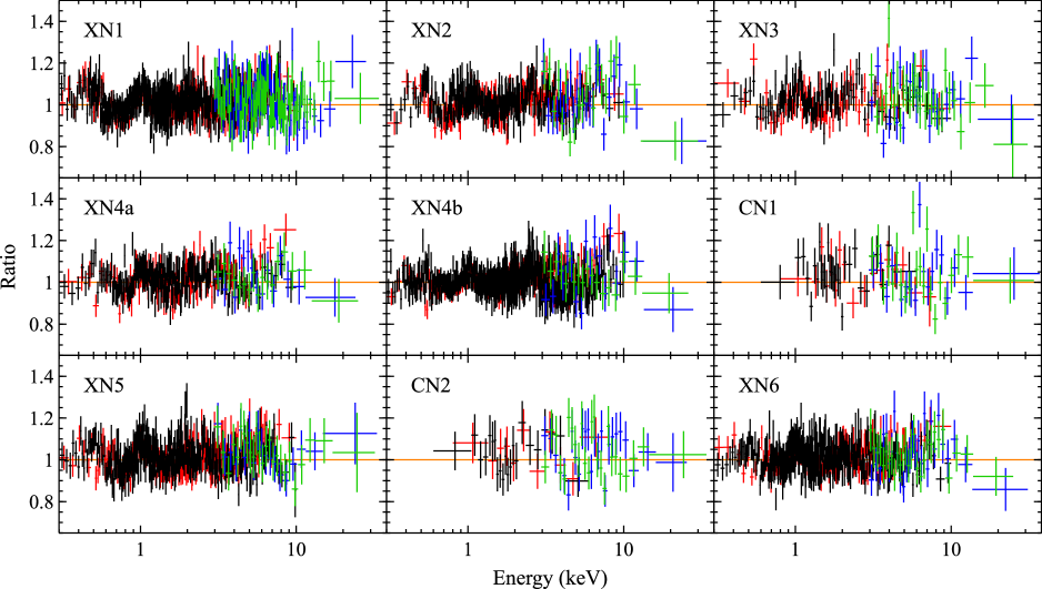
Figure 4: Data/model ratios for the nine broadband spectra extracted of NGC 1313 X-1 fit with the model assuming a non-magnetic accretor. Green and blue show data from the NuSTAR FPMA and FPMB detectors, respectively, while black and red show data from the EPIC-pn and EPIC-MOS detectors, respectively, for the XN epochs and from the MEG and HEG gratings, respectively, for the CN epochs. As with Figure 3, the data have been further rebinned for display purposes. The data/model ratios for the model assuming a magnetic accretor are extremely similar to those shown here.

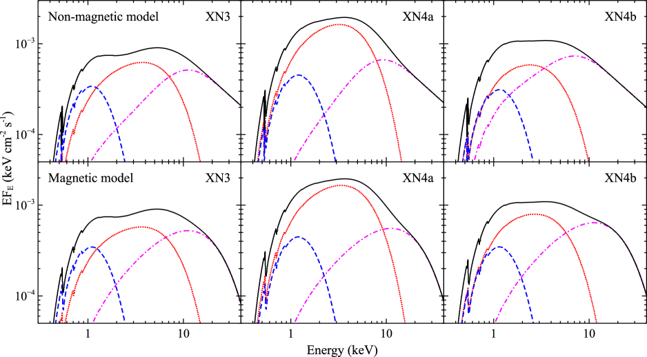
Figure 5: Example model fits for the non-magnetic accretor (top panels) and the magnetic accretor (bottom panels) models. We show the fits for epochs XN3 (representing the low-flux end of the broadband spectra; left panels), XN4a (the high-flux end of the broadband spectra, middle panels), and XN4b (one of the intermediate flux spectra; right panels). For both models, the total model is shown in solid black, the cooler DISKBB and the hotter DISKPBB components are shown in dashed blue and dotted red, respectively (in the black hole case, the DISKPBB component is shown as it would appear prior to the application of the SIMPL convolution model), and the highest energy component (either SIMPL or CUTOFFPL) is shown in dash-dot magenta. For the non-magnetic model, the contribution from SIMPL has been calculated by subtracting the unmodified DISKPBB component from the combined SIMPL$\otimes$DISKPBB contribution to the fit.

3.2.1 The Non-Magnetic Accretor Model

For super-Eddington accretion onto a non-magnetic accretor, the structure of the accretion flow is expected to deviate from the standard thin disc approximation typically invoked for sub-Eddington accretion. As the accretion rate approaches and increases beyond the Eddington limit, the scale-height of the inner regions of the disc is expected to increase, supported by the increasing radiation pressure (e.g. Shakura & Sunyaev 1973; Abramowicz et al. 1988; Poutanen et al. 2007; Dotan & Shaviv 2011). This results in a transition from a thin disc to a thicker flow roughly at the ‘spherization’ radius ($R_{\rm{sp}}$), the point at which the flow reaches the Eddington limit. Radiation pressure and potentially also advection of radiation are expected to be important for the thicker inner regions of such a flow, which modifies the radial temperature profile – typically parameterised as $T(r)\propto r^{-p}$ – of this region of the flow away from that expected for a thin disc; a standard thin disc should have $p=0.75$ (Shakura & Sunyaev 1973), while a high-Eddington, advective flow should have $p<0.75$ (Abramowicz et al. 1988). Strong winds are also expected to be launched from the regions interior to $R_{\rm{sp}}$ (e.g. Ohsuga & Mineshige 2011; Takeuchi et al. 2013), which may themselves be optically-thick (and therefore contribute blackbody-like emission) and shroud the outer accretion flow (e.g. King & Pounds 2003; Urquhart & Soria 2016; Zhou et al. 2019).

We therefore use two thermal components to model the accretion flow in the scenario that the accretor is non-magnetic, combining DISKBB (Mitsuda et al. 1984) for the outer flow/optically-thick wind and DISKPBB (Mineshige et al. 1994) for the inner flow. The DISKBB model assumes a thin disc profile (i.e. $p=0.75$), while the DISKPBB model allows $p$ to be fit as a free parameter. This combination has frequently been applied to explain the soft X-ray data ($E<10$ keV) in spectral analyses of ULXs (e.g. Stobbart et al. 2006; Walton et al. 2014, 2017; Rana et al. 2015; Mukherjee et al. 2015).

As shown in Walton et al. (2018c), even when using complex accretion disc models such as this, all the ULXs observed by NuSTAR to date – including NGC 1313 X-1 – require an additional continuum component that contributes above $\sim$10 keV. In the case of a non-magnetic accretor, this high-energy emission would likely be associated with Compton up-scattering of disc photons in a corona of hot electrons, as is the case in sub-Eddington black hole X-ray binaries and active galactic nuclei (e.g. Haardt & Maraschi 1991). We therefore model this emission with an additional high-energy powerlaw tail, using the SIMPL convolution model (Steiner et al. 2009) to avoid incorrectly extrapolating the powerlaw emission down to arbitrarily low energies. This component is applied to the DISKPBB component, the hotter of the two components associated with the disc, as black hole coronae are expected to be compact and centrally located (e.g. Reis & Miller 2013).

We apply this model to all of the 9 broadband datasets of NGC 1313 X-1 considered in this work simultaneously, similar to our analysis of Holmberg IX X-1 (Walton et al. 2017). Following that work, and given the similarities between the multi-epoch spectra at the highest and lowest energies, we assume a common absorption column (see also Miller et al. 2013) and a common photon index for the high energy continuum across all epochs. The global fit to the data is reasonably good, with $\chi^{2}$ = 12544 for 11559 degrees of freedom (DoF); we give the best-fit parameters in Table 2, and show the data/model ratios for the various datasets in Figure 4. Although there are notable residuals at $\sim$1 keV in most cases, related to atomic emission and absorption associated with the extreme outflow which are blended in the low-resolution spectra used here (Middleton et al. 2014, 2015b; Pinto et al. 2016), the shape of the continuum emission is reasonably well reproduced. We show examples of our model fits for epochs XN3, XN4a and XN4b (i.e. covering a range of fluxes) in Figure 5.

3.2.2 The Magnetic Accretor Model

The model we use for the case of a magnetic accretor (i.e. a ULX pulsar) is based on that discussed in Walton et al. (2018b, c). This consists of two thermal blackbody components for the accretion flow outside of the magnetosphere ($R_{\rm{M}}$; the point at which the magnetic field of the neutron star truncates the disk and the accreting material begins to follow the field lines instead), and an exponentially cutoff powerlaw component (CUTOFFPL) for the central accretion columns that form as the material flows down onto the magnetic poles. For the thermal components we again use the DISKBB+DISKPBB combination, which has also been used in previous work on ULX pulsars; assuming that $R_{\rm{M}}$ $<$ $R_{\rm{sp}}$, the qualitative structure of a super-Eddington flow (thin outer disc, thick inner disc, optically-thick wind) is expected to be broadly similar to the non-magnetic case for radii outside of $R_{\rm{M}}$. The discovery of the strong wind in the ULX pulsar NGC 300 ULX1 supports the conclusion that the super-Eddington regions of the accretion flow still form in these systems (i.e. $R_{\rm{M}}$ $<$ $R_{\rm{sp}}$; Kosec et al. 2018b; Mushtukov et al. 2019). For dipolar magnetic fields, this would correspond to the lower end of the predicted range of field strengths ($B\lesssim 10^{12}$). However, stronger fields could still be permitted with higher-order field geometries (e.g. Israel et al. 2017a; Middleton et al. 2019).

Since pulsations have not been detected from NGC 1313 X-1 we can not constrain the spectral shape of any accretion columns directly. We therefore take a similar approach to Walton et al. (2018c), and set its spectral parameters to the average values seen from the pulsed emission from the four ULX pulsars currently known: $\langle\Gamma\rangle=0.59$ and $\langle E_{\rm{cut}}\rangle=7.9$ keV (Brightman et al. 2016; Walton et al. 2018b, c, a). These values are similar, but are not identical to those used in Walton et al. (2018c), as NGC 300 ULX1 had not been discovered to be a ULX pulsar at that time; note that for this source we take the continuum parameters from the model that includes the cyclotron resonant scattering feature presented in Walton et al. (2018a). In the magnetised case, this component provides the bulk of the high-energy ($E>10$ keV) emission observed by NuSTAR and explains the high-energy excess seen even with complex disc models; the treatment of this emission is the only difference between the non-magnetic and magnetic accretion models used here.

As with the non-magnetic case, we apply this model to all 9 broadband datasets considered in this work simultaneously, again assuming a common absorption column for all epochs (the shape of the accretion column is fixed in the model, and so is also common for all epochs). The global fit to the data is similarly good ($\chi^{2}$/DoF = 12572/11560), with the shape of the continuum similarly well described as the non-magnetic case (we do not show the data/model ratios for the magnetic accretor model for brevity, as they are extremely similar to Figure 4), and the best-fit parameters are again presented in Table 2. We also show examples of these model fits in Figure 5; for ease of comparison, we show the same epochs as shown for the non-magnetic accretor model.

4 Discussion

We have presented a multi-epoch spectral analysis of all of the broadband datasets available for the bright ($L_{\rm{X}}\sim 10^{40}$ erg s^-1) ULX NGC 1313 X-1. These datasets combine observations taken with XMM-Newton and Chandra in coordination with NuSTAR, and span a period of $\sim$5 years. The first of these epochs, XN1, corresponds to the data presented by Bachetti et al. (2013). From these observations we extracted 9 broadband spectra, covering the $\sim$0.5–30 keV energy range, which probe the spectral variability exhibited on timescales of $\sim$days to $\sim$years (see Section 3). Several of these are broadly similar to epoch XN1 (epochs XN3, CN1, XN5, CN2), but others probe higher fluxes and show clear differences in their spectra (epochs XN2, XN4a,b, XN6; see Figure 3).

In a qualitative sense, the spectral variability exhibited by these observations is remarkably similar to that seen in Holmberg IX X-1 (see Figure 1 in Walton et al. 2017). Strong variability is apparent at low energies (below $\sim$10 keV), with the spectra showing a more flat-topped profile at lower fluxes, and becoming more centrally peaked at higher fluxes. However, at higher energies the data pinch together and remain remarkably stable. Indeed, despite the factor of $>$3 variations seen at $\sim$3 keV, the 10–40 keV fluxes only vary by a factor of at most $\sim$1.5 (see Figure 3). A similar effect may also have been seen at higher energies in the high-mass X-ray binary GX 301–2, which exhibited notable stability in the emission seen by NuSTAR above $\sim$40 keV despite clear variability at lower energies (Fürst et al. 2018).

As discussed previously, ULXs are now generally expected to represent a population of super-Eddington accretors, at least some of which are powered by neutron stars. We therefore construct spectral models that may broadly represent emission from a super-Eddington accretion flow. Such accretion flows are broadly expected to be formed of a large scale-height inner funnel, a strong wind launched by this inner funnel (which may be optically thick) and a more standard thin outer accretion disc (which may be shrouded by the wind), so our models include two multi-colour blackbody components with different temperatures, one for the inner funnel and one for the outer disc/wind. These dominate the observed spectra below $\sim$10 keV; in general, the cooler component contributes primarily below $\sim$1 keV, while the hotter component contributes primarily in the $\sim$1–10 keV band. Similar models have frequently been applied to ULX data below 10 keV (e.g. Stobbart et al. 2006; Gladstone et al. 2009; Walton et al. 2014). In the case of NGC 1313 X-1, the need for two components below 10 keV is visually apparent for the lower flux observations (Figure 3). However, even for the higher flux epochs, where this is not as obvious, the spectral decomposition found here is supported by the short-timescale variability results presented by Kara et al. (2020) for epoch XN4 (the most variable broadband epoch). The covariance analysis presented in that work clearly shows evidence for distinct spectral components above and below $\sim$2 keV (see also Middleton et al. 2015a), similar to the model used here.

However, as demonstrated by Walton et al. (2018c), when fit with such models all ULXs observed by NuSTAR to date (including NGC 1313 X-1) require an additional component at high energies to account for the NuSTAR data above $\sim$10 keV, as the Wien tail in accretion disc models falls off too steeply. Since pulsations have not currently been observed from NGC 1313 X-1, and so the nature of the accretor in this system is not currently known, we take two different approaches to modelling this additional high-energy component. First, we treat it as a high-energy powerlaw tail produced by Compton up-scattering in an X-ray corona, similar to that seen in other X-ray binary systems. We refer to this as the non-magnetic scenario, which may be appropriate for both black hole and non-magnetic neutron star accretors. Second, we treat it as high-energy emission from a super-Eddington accretion column onto a magnetised neutron star, and assume a spectral form motivated by the pulsed emission observed from the known ULX pulsars (using the average spectral shape of their pulsed spectra as a template). We refer to this as the magnetic scenario.

Walton et al. (2017) suggested that the broadband spectral variability seen in Holmberg IX X-1, similar to that reported here for NGC 1313 X-1, could potentially be related to the presence of the expected funnel-like geometry for the inner accretion flow. In such a scenario, the funnel is expected to geometrically collimate the emission from the innermost regions within the funnel (discussed further in Section 4.2). Regardless of the nature of the accretor (black hole or neutron star), the highest energy emission probed by NuSTAR is usually expected to arise from these regions, either powered by a centrally located Compton-scattering corona (e.g. Reis & Miller 2013), or a centrally located accretion column. The stability of this emission would therefore imply that any geometrical collimation it experiences remains roughly constant, despite the change in observed broadband X-ray flux (which would suggest a change in accretion rate, $\dot{M}$). In principle, an increase in accretion rate would be expected to result in an increase in the scale-height of the funnel (e.g. King 2008; Middleton et al. 2015a). However, while this must happen over some range of $\dot{M}$ in order for the disc structure to transition from the thin disc expected for standard sub-Eddington accretion to the funnel-like geometry expected for super-Eddington accretion, as discussed by Lasota et al. (2016), once the disc reaches the point of being fully advection-dominated the opening angle of the disc should tend to a constant ($H/R\sim 1$, where $H$ is the scale-height of the disc at radius $R$). Walton et al. (2017) speculated that once this occurs, rather than closing the funnel further, an increase in $\dot{M}$ instead simply increases the characteristic radius within which geometric beaming occurs, such that emission that is already within this region (the highest energies probed) experiences no further collimation with an increase in $\dot{M}$, while emission from larger radii (i.e. from more intermediate energies) does still become progressively more focused, and would exhibit stronger variability. In essence, this idea invokes a radially-dependent beaming factor in which the beaming of the innermost regions has saturated to explain (in only a qualitative sense) the unusual, energy-dependent broadband spectral evolution seen from Holmberg IX X-I (and now NGC 1313 X-1).

4.1 Evolution of the Thermal Components

With this picture in mind, and with a fairly extensive, broadband dataset now available for NGC 1313 X-1, we consider the behaviour of the two thermal components in each of our models in detail. In particular, we investigate how the DISKBB and DISKPBB components evolve in the luminosity–temperature plane. To compute the luminosity, we calculate the intrinsic fluxes (i.e. absorption corrected, and in the case of the DISKPBB component for the black hole model, corrected for the photons lost to the powerlaw tail) for each of the thermal components individually, computed over a broad enough band to be considered bolometric (0.001–100 keV). The results for each component are shown in Figure 6 for both of the models considered.

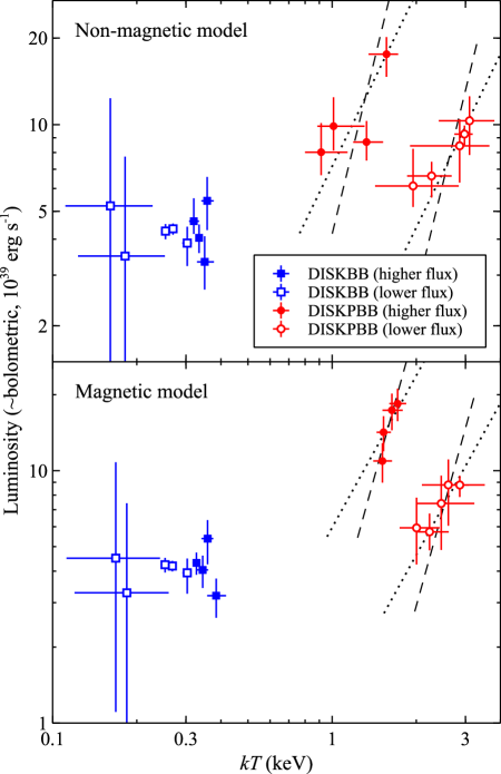
Figure 6: 0.001–100 keV (i.e. $\sim$bolometric) luminosity vs temperature for both the DISKBB (blue squares) and DISKPBB (red circles) components from our multi-epoch spectral analysis with the models assuming the accretor is non-magnetic (top) and magnetic (bottom). No clear relation is seen for the DISKBB component (although this may be related to modelling issues, see Section 4). However, in both cases the results for the DISKPBB component appear to show distinct tracks at high and low luminosities (observed fluxes above and below $F^{\rm{obs}}_{0.3-40.0}=5\times 10^{-12}$ $\rm\thinspace erg~{}cm^{-2}~{}s^{-1}$; full and open symbols, respectively), both of which are broadly consistent with $L\propto T^{4}$ (indicated with the dashed lines), and also with $L\propto T^{2}$ (dotted lines).

We do not find any clear relationship between $L$ and $T$ for the lower temperature DISKBB component. However, this is likely related, at least in part, to our treatment of the hotter component with the DISKPBB model. This extends the run of temperatures down to arbitrarily low values, which is not physically reasonable if the two thermal components do represent radially distinct regions of the disc. This extrapolation will naturally influence the flux of the cooler DISKBB component, and could certainly serve to artificially mask any such relation, so the results presented here are not particularly well suited for addressing this issue for the cooler component. Indeed, based on archival XMM-Newton data, we note that Miller et al. (2013) find evidence for a positive relation between luminosity and temperature for the cooler DISKBB component when treating the higher energy emission with a Comptonization model, and assuming that the seed photons come from the DISKBB component (such that this emission has a low-energy cutoff at the DISKBB temperature). Miller et al. (2013) may therefore present a more accurate assessment of the evolution of this cooler thermal component. This issue will be explored further in future work.

The most interesting results are instead seen for the hotter DISKPBB component. In both cases (the models for non-magnetic and magnetic accretors) the results cluster into two groups, split by the observed flux. The higher-flux cases ($F^{\rm{obs}}_{0.3-40.0}>5\times 10^{-12}$ $\rm\thinspace erg~{}cm^{-2}~{}s^{-1}$; epochs XN2, XN4a,b, XN6) show lower temperatures on average, while the lower-flux cases ($F^{\rm{obs}}_{0.3-40.0}<5\times 10^{-12}$ $\rm\thinspace erg~{}cm^{-2}~{}s^{-1}$; epochs XN1, XN3, XN5, CN1, CN2) show higher temperatures. Naively, one could conclude that luminosity and temperature are inversely correlated for this component, as also discussed for Holmberg IX X-1 by Walton et al. (2014). However, when considered separately, each of these groups appear to exhibit a positive correlation (see Figure 6). We present Pearson’s correlation coefficients ($\rho$) and null hypothesis probabilities (i.e. the probability of no correlation; $p_{\rm{null}}$) in Table 3. Although the data are visually compelling, the formal statistical evidence for a correlation is not as strong for the higher luminosity/lower temperature group, in large part because this group is only made up of 4 epochs (although we note that for the non-magnetic accretor model, the evidence for a correlation is driven purely by epoch XN4a). Ultimately, further observational data will be required to robustly confirm this behaviour.

Table 3: Pearson’s correlation coefficients and null hypothesis probabilities (no correlation) for the low- and high-temperature tracks for the DISKPBB component seen in Figure 6 for the non-magnetic and the magnetic accretor models.

	Low Temp.		High Temp.
Model	$\rho$	$p_{\rm{null}}$	$\rho$	$p_{\rm{null}}$
Non-Magnetic Accretor	0.77	0.23	0.97	0.005
Magnetic Accretor	0.87	0.13	0.91	0.03

Nevertheless, each of the two groups of observations are broadly consistent with following their own distinct $L\propto T^{4}$ relationship, which would be expected for blackbody radiation with a constant emitting area. Although the qualitative results regarding e.g. temperature do depend on the choice of model, and the global uncertainties are larger in the black hole model because the shape of the high-energy continuum is free to vary in this case, qualitatively this behaviour appears to be largely model independent, as it is seen for both of the models considered. We have also performed a series of other tests related to the models used, including allowing the neutral absorption column to vary between epochs (following Middleton et al. 2015a), replacing the cooler DISKBB component with a single-temperature blackbody and linking $p$ across all of the datasets in the magnetic model, and allowing for different photon indices for the two groups of observations in the non-magnetic model. We still see qualitatively consistent behaviour in the hotter DISKPBB component to that shown above in all of these cases. In addition, we also further tested whether the spectral variability inferred for the DISKPBB component within each group of observations is really required by the data, as this drives the two positive luminosity–temperature correlations seen in Figure 6. To do so we re-fit the data assuming common values for both $p$ and $T_{\rm{in}}$ for the DISKPBB component for the observations that make up each group, allowing only for the flux of this component to vary within them. This significantly degrades the fit by $\Delta\chi^{2}\sim 100$ (for 14 fewer free parameters) for both the non-magnetic and the magnetic accretor models; F-tests imply the probabilities of these differences in fit statistic occurring by chance are $\sim$10^-12 in both cases.

Given the concerns regarding the extrapolation of the DISKPBB model mentioned above, we also investigated whether the results for this component shown in Figure 6 could be influenced by extending this component significantly outside of the observed bandpass. Instead of using the broader 0.001–100 keV fluxes shown in Figure 6, we also compute the fluxes for this model component above 1 keV, which is primarily covered by the observed bandpass. Although the quantitative details naturally change, the same qualitative behaviour is still seen: the observations split into two distinct groups with their own luminosity–temperature tracks, each of which are consistent with $L\propto T^{4}$. In the non-magnetic case the results for this higher energy band are again not as clear-cut as the magnetic case, but the data are also still consistent with there being two groups following separate tracks, each again consistent with $L\propto T^{4}$. The observed behaviour therefore appears to be largely robust to any issues regarding extrapolation of the DISKPBB component outside of the observed bandpass. We also note that this demonstrates that the atomic features associated with the wind, which are not modelled here, do not significantly influence the observed luminosity–temperature behaviour for the DISKPBB component, as these features have a very small effect on the DISKPBB flux above 1 keV (at the level of a few per cent; Pinto et al. 2020).

Owing to the small number of observations and the relatively limited dynamic range currently available for each track, we do not fit for formal luminosity–temperature relations at this stage. Instead, to test for the consistency with $L\propto T^{4}$ in a simple manner, we perform some further fits to the data in which we assume constant inner radii ($R_{\rm{in}}$) for the DISKPBB component for each of the two groups of observations. Formally we link their normalisations, which are given by $[R_{\rm{in}}/(\xi Df_{\rm{col}}^{2})]^{2}\cos(i)$, where $R_{\rm{in}}$ and $D$ are in units of km and 10 kpc, respectively, $i$ is the inclination of the disc, $f_{\rm{col}}$ is its colour correction factor, and $\xi$ is a further correction introduced by the inner boundary condition assumed in the DISKBB/DISKPBB models ($\xi\sim 0.4$; Kubota et al. 1998; Vierdayanti et al. 2008). The colour correction factor is a simple multiplicative correction designed to empirically account for the complex atmospheric physics in the disc by relating its ‘colour’ temperature at the photosphere ($T_{\rm{col}}$) to its effective blackbody temperature ($T_{\rm{eff}}$), and is defined as $T_{\rm{col}}=f_{\rm{col}}T_{\rm{eff}}$. Assuming that $i$ and $f_{\rm{col}}$ are similar for the DISKPBB component for both groups of observations, the ratio of their inner radii is simply related to the ratio of their normalizations, i.e. $R_{\rm{in,1}}/R_{\rm{in,2}}=\sqrt{\rm{Norm}_{1}/\rm{Norm}_{2}}$ (where subscripts 1 and 2 refer to the lower and higher temperature tracks, respectively). Although we now have seven fewer free parameters, these fits are only worse by $\Delta\chi^{2}$ = 21 and 15 for the non-magnetic and magnetic models, respectively, and we find that the ratios of the two radii are $R_{\rm{in,1}}/R_{\rm{in,2}}=4.6^{+1.2}_{-1.0}$ and $3.6^{+0.6}_{-0.7}$.

We also estimate the minimum inner radii (in the context of isotropic emission) for the DISKPBB component implied by the two potential $L\propto T^{4}$ tracks by assuming no colour correction (i.e. $f_{\rm{col}}=1$) and a face-on inclination (i.e. $i=0$). For the non-magnetic model, these inner radii are $R_{\rm{in,1}}\sim 26$ km and $R_{\rm{in,2}}\sim 5.6$ km, while for the magnetic model these inner radii are $R_{\rm{in,1}}\sim 19$ km and $R_{\rm{in,2}}\sim 5.2$ km. We stress that any colour correction and/or non-zero inclination will increase these estimates. Although the colour correction is typically taken to be $f_{\rm{col}}=1.7$ for sub-Eddington accretion (e.g. Shimura & Takahara 1995), for super-Eddington accretion $f_{\rm{col}}\sim 3$ may be more appropriate (Watarai & Mineshige 2003, Davis & El-Abd 2019, and in reality $f_{\rm{col}}$ may have a radial dependence, Soria et al. 2008). Adopting this value and an inclination of $i=60$^∘, for example, increases these estimates by a factor of $3^{2}/\sqrt{0.5}\approx 12.7$ to $R_{\rm{in,1}}\sim 320$ km and $R_{\rm{in,2}}\sim 71$ km for the non-magnetic model, and to $R_{\rm{in,1}}\sim 240$ km and $R_{\rm{in,2}}\sim 66$ km for the magnetic model. If the accretor is a 10 $\rm M_{\odot}$ black hole, these radii would correspond to $R_{\rm{in,1}}\sim 20$ $R_{\rm{G}}$ (where $R_{\rm{G}}$ $=GM/c^{2}$ is the gravitational radius) and $R_{\rm{in,2}}\sim 5$ $R_{\rm{G}}$, and if the accretor is a $\sim$1.4 $\rm M_{\odot}$ neutron star they would correspond to $R_{\rm{in,1}}\sim 115-150$ $R_{\rm{G}}$ and $R_{\rm{in,2}}\sim 30$ $R_{\rm{G}}$. In this latter case (1.4 $\rm M_{\odot}$ neutron star), the radii inferred are vaguely similar to the launching radii for the two main components of the wind inferred by Pinto et al. (2020), based on escape velocity arguments ($\sim$50 and $\sim$300 $R_{\rm{G}}$, i.e. within a factor of $\sim$2). In the former (10 $\rm M_{\odot}$ black hole), all of the changes inferred here would appear to be occurring interior to the wind launching regions based on the same arguments, although the larger radius is similarly comparable to the innermost radius for the wind (again within a factor of $\sim$2).

It is important to note that the two groups of observations that show these different $L\propto T^{4}$ tracks do not simply represent distinct periods of time over which these different emitting radii remained stable. Instead, the source appears to switch back-and-forth between them. The cadence of our broadband sampling is not particularly constraining with regards to the transition between these two tracks; from these data we can only determine that NGC 1313 X-1 is able to move between them in the space of a few weeks (the time between epochs XN4 and CN1). Should these two tracks represent intrinsic evolution in the DISKPBB component, these two radii would therefore imply that there are two stable geometric configurations that NGC 1313 X-1 repeatedly returns to/transitions between. It is also important to note that the epochs exhibiting higher observed luminosities also show the larger of the two radii. This makes it unlikely the observed behaviour is related to bulk precession of an otherwise stable (i.e. constant accretion rate) large scale-height inner flow changing our ability to view the emission from its innermost regions (e.g. Middleton et al. 2018). In this scenario, the smaller inner disc radii should be observed when we can see further into the funnel, and therefore be associated with higher observed fluxes. Furthermore, there is no hint that the long-term variability exhibited by NGC 1313 X-1 is even quasi-periodic (Figure 1), instead exhibiting a marked increase in seemingly aperiodic variability after MJD $\sim$ 57400 (as noted previously).

Given the presence of the two luminosity–temperature tracks, we also explore the possibility that there are actually two distinct thermal components (each producing one track) that are always present and, in combination, dominate the $\sim$1–10 keV band (such that the $\sim$0.3–40 keV spectrum would actually be made up of four continuum components, instead of the three used in our previous modelling). This might, for example, represent a scenario in which there is even further radial segregation of the accretion flow than included in our baseline models (see Section 4.5 for further discussion). In this picture, these two thermal components exhibit different levels of long-term variability, such that their relative contribution changes from epoch to epoch, and in our 3-component models the DISKPBB component is forced to (and has sufficient flexibility to) primarily account for whichever of these two components dominates the $\sim$1–10 keV band for any particular epoch, switching its apparent properties between the two as necessary. For brevity and simplicity, we focus on the magnetized accretor model and replace the DISKPBB component with two standard DISKBB accretion disc models, each of which has a normalisation linked across all the epochs considered (i.e. we assume each new DISKBB component varies following $L\propto T^{4}$). As such, the full continuum model in this case consists of 3 DISKBB components and the CUTOFFPL component associated with the accretion column. This actually provides a reasonable improvement to the fit obtained with the 3-component model, with $\chi^{2}$/DoF = 12454/11567 (i.e. $\Delta\chi^{2}=118$ for 7 additional free parameters); the temperatures of the two new DISKBB components vary from $kT_{1}\sim 0.6-1.0$ keV and from $kT_{2}\sim 1.9-2.5$ keV, respectively. In this case, the ratio of the inner radii of the two new DISKBB components is $R_{\rm{in,1}}/R_{\rm{in,2}}=6.4\pm 0.6$, and the minimum possible inner radii (again assuming no colour correction and a face-on inclination) inferred are $R_{\rm{in,1}}\sim 75$ km and $R_{\rm{in,2}}\sim 12$ km. We stress that these radii should be taken with a large degree of caution, as the issues regarding extrapolation of the individual thermal models to low energies discussed above are even further exacerbated in this case; the values are primarily presented for completeness and reproducibility.

Although the luminosity–temperature tracks returned by our analyses are consistent with $L\propto T^{4}$, in most cases they are also consistent with flatter luminosity–temperature relations. In particular, most tracks are also consistent with $L\propto T^{2}$ (also shown in Figure 6), which, even if $R_{\rm{in}}$ remains $\sim$constant, may be expected for the inner regions of an advection-dominated disc around a black hole (in which some of the radiated flux from these regions is trapped by the flow and carried across the event horizon, e.g. Watarai et al. 2000; note that this is not possible for a neutron star accretor, as in that case the radiation must emerge in some form). Some Galactic black hole X-ray binaries are seen to transition to a luminosity–temperature relation similar to $L\propto T^{2}$ at high luminosities (see e.g. Kubota & Makishima 2004; Abe et al. 2005), and some ULXs also show evidence for this behaviour (Walton et al. 2013). Similar to the $L\propto T^{4}$ case, we perform additional fits where the normalisations of the DISKPBB component are linked across each of the two groups of observations in a manner that would give $L\propto T^{2}$; again with seven fewer free parameters, we find the fits are only worse by $\Delta\chi^{2}$ = 31 and 30 for the non-magnetic and magnetic models, respectively. The global fits are therefore marginally worse than (but still essentially comparable to) the fits assuming $L\propto T^{4}$. Given the limited dynamic range covered by each of the tracks, the radii estimated above assuming $L\propto T^{4}$ are likely still representative of the characteristic emitting radii that would be inferred for each of the two groups of observations even if $L\propto T^{2}$. However, since in this case the ‘true’ disc luminosity is underestimated (as some fraction is advected over the horizon), the absolute radii would likely be underestimated (see e.g. Kubota & Makishima 2004).

In the following sections, we discuss potential physical causes for the two distinct luminosity–temperature tracks associated with the DISKPBB component, and also explore potential scenarios in which stable emitting radii could be produced in the accretion flow for NGC 1313 X-1.

4.2 Geometric Collimation and Disc/Wind Scale-Height

The above estimates for the emitting radii do not account for any geometric collimation of the radiation that might be experienced by the emission from these thermal components. As discussed previously, this may be expected for the inner regions of a super-Eddington accretion flow, which, through the combination of the outer disc and the wind, should form a funnel-like geometry. Should any of the thermal emission arise from regions interior to this inner funnel then it should be collimated into a solid angle set by the opening angle of this funnel, $\Omega$. By assuming no collimation, the total luminosity emitted and in turn the emitting radii would be overestimated. Introducing a ‘beaming’ factor of $b=\Omega/4\pi$, such that the ‘observed’ luminosity inferred assuming isotropic emission, $L_{\rm{obs}}$, and the actual emitted luminosity, $L_{\rm{int}}$, are related via $L_{\rm{int}}=bL_{\rm{obs}}$ (following King 2008, such that $b\leq 1$; we assume here that we are looking down the funnel), then should any of the thermal emission be collimated the radii inferred from this emission would need to be corrected by a factor $\sqrt{b}$.

Furthermore, any variations in the degree of beaming $b$ would manifest as changes in the emitting areas/radii in our analysis. Indeed, if we consider the case where there is more collimation of a blackbody thermal component at higher intrinsic luminosities, as may be expected for a disk which has a larger scale-height at higher accretion rates, we can write $b\propto L_{\rm{int}}^{-\beta}$, where $\beta>0$ (as more collimation corresponds to smaller $b$ in our definition). Assuming that the intrinsic emission behaves as $L_{\rm{int}}\propto T^{\alpha}$, and that the process of collimation does not also change $T$ (i.e. $T_{\rm{int}}=T_{\rm{obs}}=T$; this will be discussed further in Section 4.4), combining this with the definition of $b$ and the scaling between $b$ and $L_{\rm{int}}$ we find that $L_{\rm{obs}}\propto T^{\alpha(1+\beta)}$. Non negligible $\beta$ could therefore produce clear deviations from $L_{\rm{obs}}\propto T^{4}$ for a constant area blackbody, with a steeper luminosity–temperature scaling expected in this particular scenario. If both $L_{\rm{obs}}\propto T^{4}$ and $L_{\rm{int}}\propto T^{4}$, or both $L_{\rm{obs}}\propto T^{2}$ and $L_{\rm{int}}\propto T^{2}$, then $b$ must be constant. Alternatively, it would still be possible to produce $L_{\rm{obs}}\propto T^{4}$ even if $L_{\rm{int}}\propto T^{2}$ provided that $b\propto L_{\rm{int}}^{-1}$. However, in any of these cases, in order to produce two distinct groups in the luminosity–temperature plane purely through beaming, there would need to be a sharp transition in $b$ at some point. This is naturally problematic for any model invoking progressive changes in the opening angle of a large scale-height inner flow. In addition to being problematic for models invoking progressive changes in the scale-height of the disc, it is similarly unclear how the picture of a progressively changing radial beaming profile suggested by Walton et al. (2017) for Holmberg IX X-1 would be able to explain the two distinct groups of observations seen for NGC 1313 X-1.

A model invoking a larger scale-height at higher accretion rates could instead potentially produce a sharp transition in the luminosity–temperature plane should our viewing angle be close to the opening angle of the flow at lower luminosities, such that by increasing the scale-height of the disc/wind the innermost regions of the flow are suddenly obscured by the regions at larger radii, resulting in a larger inner radius being inferred at higher luminosities. For this to be a plausible explanation for the broadband behaviour, the obscuring regions would need to correspond to those contributing the lower temperature parts of the DISKPBB component that are still visible in the higher flux observations. A toy model for the transition in the luminosity–temperature plane in this scenario is shown in Figure 7 (left). However, if the thermal emission from the inner regions of the disc is suddenly obscured, one would naturally expect a central corona/accretion column to be similarly obscured, but the high-energy NuSTAR data are rather stable.

4.3 Scattering Losses in a Wind

Alternatively, it may be the case that the high-temperature track is actually a smooth continuation of the low-temperature track, but that above some observed luminosity we view the emission through an ionised disc wind, which results in an apparent decrease in the observed flux due to losses associated with electron scattering. A toy model for the transition in the luminosity–temperature plane in this scenario is also shown in Figure 7 (right). Indeed, NGC 1313 X-1 is now known to launch a powerful disc wind (Middleton et al. 2015b; Pinto et al. 2016, 2020), which at least at times has a highly-ionised component along our line-of-sight (Walton et al. 2016a). To test this scenario we perform some further fits in which we assume a single normalisation for the DISKPBB component for all epochs, and apply a CABS component to this emission for the observations that make up the higher-temperature track, again focusing on the magnetic accretor model for brevity. CABS accounts for flux losses due to electron scattering, and is characterised by an effective column density for the scattering medium, which we link across the high-temperature observations in order to preserve a common intrinsic $L_{\rm{obs}}\propto T^{4}$ scaling for both the high- and low-temperature tracks. We find that this provides an equivalently good fit to the model with two linked DISKPBB normalisations (see Section 4.1), with $\chi^{2}$/DoF = 12604/11567, and that the scattering column density required to bring about the drop in flux inferred from an extrapolation of the low-temperature track to the observed high-temperature track is $N_{\rm{H}}=3.1^{+0.3}_{-0.4}\times 10^{24}$ $\rm\thinspace cm^{-2}$.

The scattering column required is significantly larger than the best-fit column densities inferred for any of the components of the wind in NGC 1313 X-1 reported to date. For the moderately ionised components that contribute the features detected at $\sim$1 keV by the RGS, $N_{\rm{H}}\sim 10^{21-22}$ $\rm\thinspace cm^{-2}$ (Pinto et al. 2016, 2020) For the highly ionised component that provides the iron K absorption seen in archival XMM-Newton and NuSTAR data (which are primarily made up of epoch XN1), $N_{\rm{H}}\sim 10^{23}$ $\rm\thinspace cm^{-2}$ (Walton et al. 2016a), although it is worth noting that there is a local minimum in the parameter space for the highly ionised component that does extend up to column densities comparable to that inferred above ($N_{\rm{H}}\sim 10^{24}$ $\rm\thinspace cm^{-2}$). Fixing the CABS column density to $10^{23}$ $\rm\thinspace cm^{-2}$ in this scenario significantly degrades the fit ($\Delta\chi^{2}$ = 165 for one fewer free parameter, giving a negligible F-test probability of a chance improvement), as the scattering losses are very small; the CABS component is therefore unable to reproduce the required drop in flux, and the model instead tries to produce this drop by introducing large differences in $p$ for the two groups, resulting in a notably worse fit.

Figure 7: Toy models for the luminosity–temperature plane for the scenarios in which the inner disc is suddenly fully obscured by the outer disc/wind (left panel; discussed in Section 4.2) and in which the emission from the inner disc is scattered by a highly ionised wind which still permits some of the emission to escape (right panel; discussed in Section 4.3).

As noted above, this scenario would require there to be a sharp transition in the wind properties along our line-of-sight to explain the observed behaviour. Furthermore, if both tracks follow $L_{\rm{obs}}\propto T^{4}$, or both follow $L_{\rm{obs}}\propto T^{2}$, then the wind properties would need to be bi-modal, such that we are either viewing the central regions through a negligible scattering column, or through basically the same column whenever our line-of-sight intercepts the wind. Although Middleton et al. (2015b) do find that the residuals at $\sim$1 keV imprinted by the wind are weaker in archival XMM-Newton observations that would lie on the higher-flux, lower temperature track, the evolution appears to be a continuous function of the observed hardness of the source. Indeed, Pinto et al. (2020) find that, although there are some differences in the properties of the wind between observations in the two tracks, both still show broadly similar absorption from the moderately-ionised components in the RGS data. In order for this scenario to be plausible, the local minimum at $N_{\rm{H}}\sim 10^{24}$ $\rm\thinspace cm^{-2}$ reported in Walton et al. (2016a) would likely need to be the correct solution, and this highly ionised component would also need to show much stronger variability between the two tracks than these more moderately ionised components. The work so far on the wind properties in the new 2017 campaign has focused on the RGS band, and is not particularly sensitive to the highly ionised component that would be most relevant for this scenario (the current absorption analysis does not exclude this scenario, Pinto et al. 2020); this will be further addressed in future work. Alternatively, it could be that the scattering medium is a fully ionised component of the wind, such that it does not imprint any discernible absorption features. However, fully ionising a column of $N_{\rm{H}}\sim 3\times 10^{24}$ $\rm\thinspace cm^{-2}$ such that there is no significant absorption opacity below 10 keV is obviously challenging, particularly if the DISKBB temperature ($\sim$0.2–0.4 keV) represents the characteristic temperature of the wind. Regardless, as with the scenario in which the outer disc fully blocks the inner disc, it is similarly difficult to explain the lack of strong long-term variability at the highest energies in this scenario under the assumption that this emission comes from the most compact regions.

4.4 The Colour Correction Factor and Down-Scattering

Beyond geometric considerations, which all have difficulty explaining the stability of the highest energy emission, it may also be possible to produce two apparently distinct luminosity–temperature tracks by varying the colour correction factor, $f_{\rm{col}}$, introduced by the atmosphere of the disc (previously we assumed a single value for all of the available data). However, similar to the above cases, in order to do so $f_{\rm{col}}$ would need to have two distinct values that it varies between, or at the very least exhibit a sharp jump at some point in its evolution with accretion rate. This would result in a sudden change in the observed temperature at a given luminosity. However, none of the works that have tried to consider how this should vary with accretion rate have shown an obvious indication for such a sudden jump (Shimura & Takahara 1995; Davis & El-Abd 2019). Furthermore, the general expectation among these works is that $f_{\rm{col}}$ should increase with increasing accretion rate, which should result in the highest temperatures being observed at the highest luminosities. Again, this is not the case, so it is not clear that this is a realistic possibility either.

In addition to the atmospheric corrections associated with the disc, if the emission from the inner regions is geometrically collimated by the outer disc/wind, the cooler temperatures associated with these regions could result in significant down-scattering (e.g. Middleton et al. 2015a). This would lower the temperature observed even if the bulk of the scattering occurs away from our line-of-sight, such that $T_{\rm{col}}=f_{\rm{ds}}T_{\rm{obs}}$, where $f_{\rm{ds}}\geq 1$ (we parameterise this separately as $f_{\rm{ds}}$ to make the distinction with $f_{\rm{col}}$). As the wind launching radius should increase with increasing accretion rate (see Section 4.5), we might expect a scenario in which there the down-scattering introduces a larger effect at higher luminosities, such that $f_{\rm{ds}}\propto L^{\gamma}$ with $\gamma>0$. For a given luminosity–temperature relationship prior to any down-scattering of the form $L\propto T_{\rm{col}}^{\alpha}$, and neglecting the effects of beaming here, we find that increasingly strong down-scattering at higher luminosities should modify the observed luminosity–temperature relation to $L\propto T_{\rm{obs}}^{\alpha/(1-\alpha\gamma)}$. This kind of down-scattering relation would therefore either steepen the observed luminosity–temperature relation if the trend remains positive (since this requires $\alpha\gamma<1$), or reverse the trend to give a negative luminosity–temperature relation. This may therefore provide another means by which it would be possible to have observed $L_{\rm{obs}}\propto T_{\rm{obs}}^{4}$ even if $L_{\rm{int}}\propto T_{\rm{int}}^{2}$. However, as with all of the other scenarios considered, producing the two groups of observations would require a sharp jump in the degree to which down-scattering influences the observed emission, and our naive expectation is that this should vary smoothly with accretion rate. Furthermore, reprocessing of the emission from the inner regions by the outer disc/wind is generally considered to be related to the lowest temperature emission (i.e. the DISKBB component) given the apparent connection between ULXs and ultraluminous supersoft sources (ULSs; e.g. Urquhart & Soria 2016; Pinto et al. 2017).

4.5 Super-Eddington X-ray Binaries: Key Radii

Having considered a variety of different possible mechanisms by which the two luminosity–temperature tracks could be produced by either geometric or atmospheric corrections to the inner disc emission, none of which are particularly compelling, we now consider the possibility that we are seeing further distinct key radii/regions of the accretion flow even within the energy range covered by the DISKPBB component in our models. For super-Eddington accretion onto either a black hole or a neutron star there are several key radii to consider: the inner edge of the disc, the spherization radius ($R_{\rm{sp}}$; the point at which the disc transitions from a standard thin outer disc to the thick inner disc expected for super-Eddington accretion, which should also correspond to the point at which strong, radiatively-driven winds start to be launched), and the photon trapping radius ($R_{\rm{trap}}$, the radius interior to which photons are primarily advected inwards rather than released locally; note that $R_{\rm{trap}}$ $<$ $R_{\rm{sp}}$, Poutanen et al. 2007).

4.5.1 Black Hole Accretor

For a black hole accretor, the accretion disc is expected to extend in to the innermost stable circular orbit ($R_{\rm{ISCO}}$) at high accretion rates. This is set purely by the mass and spin of the black hole, neither of which can be changing significantly over the course of the observations considered here, so the inner regions of the accretion flow would be expected to have a constant inner radius even if the accretion rate onto the black hole changes. $R_{\rm{ISCO}}$ would therefore be a natural candidate for the smaller of the two potential stable radii in NGC 1313 X-1 ($R_{\rm{in,2}}$; we note again that, even if $L\propto T^{2}$ for these observations, this would imply a stable inner radius if the disc is in the advection-dominated regime). Indeed, the rough estimates for the absolute value of this radius are appropriate for the innermost stable circular orbit of a typical 10 $\rm M_{\odot}$ black hole, depending on its spin.

However, in contrast to $R_{\rm{ISCO}}$, based on standard accretion theory the spherization radius is expected to scale with the accretion rate, i.e. $R_{\rm{sp}}$ $\propto$ $\dot{m}$ (where $\dot{m}$ is the accretion rate in units of the Eddington accretion rate; Shakura & Sunyaev 1973; Poutanen et al. 2007). The trapping radius is also expected to have a similar dependence, i.e. $R_{\rm{trap}}$ $\propto$ $\dot{m}$ (Lasota 2016). Should the lower-temperature track exhibit a constant radius, and be related to either of these radii in the flow, this would imply that the accretion rate is constant. However, changes in $\dot{m}$ are almost certainly required to produce the flux and temperature variations observed. Allowing instead for a varying emitting radius that increases with luminosity, as would be expected for both $R_{\rm{sp}}$ and $R_{\rm{trap}}$, we can write $R\propto L^{\delta}$ (where $\delta>0$), and show that in this case $L\propto T^{4/(1-2\delta)}$ (assuming $L\propto R^{2}T^{4}$, since we are considering the regions outside $R_{\rm{trap}}$). This scenario should either again steepen the observed luminosity–temperature relation away from $L\propto T^{4}$ (for $0<\delta<0.5$) or even reverse the trend such that $L_{\rm{obs}}$ and $T$ are anti-correlated (for $\delta>0.5$). Given that positive correlations are observed, we may therefore expect the lower temperature track to have a steeper luminosity–temperature relation than the higher temperature track if this is associated with either $R_{\rm{sp}}$ or $R_{\rm{trap}}$, particularly if the inner regions vary as $L\propto T^{2}$. Although the data do not obviously require this, given the limited observations we cannot exclude this possibility (and there is maybe a weak hint that this is the case for the results from the magnetic model). However, if the effects of e.g. beaming are more pronounced for the higher-temperature track, then this difference could be reduced.

Assuming that the DISKBB component comes from the disc/wind at the transition to the super-Eddington flow at $R_{\rm{sp}}$, one interesting possibility is therefore that we are seeing a further transition in the disc at $R_{\rm{trap}}$ manifested in the behaviour of the DISKPBB component. The decreased variability at high energies could then be a result of higher accretion rates leading to both stronger winds and increased photon trapping, such that mass accretion rate fluctuations in the outer disc lead to a much weaker response than would naively be expected from the inner regions, as discussed in Middleton et al. (2015a). This could also be qualitatively similar to the high-energy ‘saturation’ effects discussed by Feng et al. (2019).

4.5.2 Non-Magnetic Neutron Star Accretor

For a neutron star accretor, the inner edge of the accretion flow is either set by the surface of the neutron star for non- or weakly-magnetised neutron stars (modulo the presence of any boundary layer; the innermost stable circular orbit is likely similar to or smaller than the radius expected for a typical neutron star: $R_{\rm{ISCO}}$ $\sim$ 12 km, while $R_{\rm{NS}}$ $\sim$ 13 km; Miller et al. 2019; Riley et al. 2019) or the magnetospheric radius for strongly-magnetised neutron stars ($R_{\rm{M}}$; the point at which the magnetic field of the neutron star truncates the disc and the in-falling material is forced to follow the field lines instead). Similar to $R_{\rm{ISCO}}$, the radius of the neutron star cannot be evolving significantly over the course of our observations, so this may also be a plausible explanation for one of the potentially stable radii if the neutron star is non-magnetic. While the value of the inner radius estimated for the smaller of the two potential stable radii ($R_{\rm{in,2}}$) is larger than the characteristic radius expected for a neutron star, it may still be possible for the potential geometric beaming effects discussed above to bring the two into consistency (although this would require $0.05\lesssim b\lesssim 1$, depending on $f_{\rm{col}}$ and $i$, and the lower end of this range would represent moderately extreme beaming).

However, unlike the black hole case, radiation cannot be advected over the horizon here; while advection may still be a relevant process within some regions of the disc, this radiation must emerge somewhere, presumably in the boundary layer where the disc meets the neutron star surface. If this boundary layer behaves as an extension of the disc, it is not clear that it would be possible for such a scenario to produce an $L\propto T^{2}$ scaling; even with advection $L\propto T^{4}$ may be expected in this case. Alternatively, though, this boundary layer may be the origin of the highest energy emission observed by NuSTAR (i.e. $E>10$ keV), as the material shocks at the neutron star surface. If this is the case, it may still be possible for an advection-dominated disc around a neutron star to produce $L\propto T^{2}$, and we may again expect the lower temperature track to have a steeper luminosity–temperature relation. However, in this case the lack of long-term high-energy variability would likely imply that the winds are removing the majority of any accretion rate fluctuations before they reach these regions (Middleton et al. 2015a).

4.5.3 Magnetic Neutron Star Accretor

In the classic picture of accretion onto a magnetized neutron star, $R_{\rm in}$ = $R_{\rm{M}}$, and $R_{\rm{M}}$ is set by the combination of the magnetic field of the neutron star and the accretion rate: $R_{\rm{M}}$ $\propto B^{4/7}\dot{M}^{-2/7}$ (Lamb et al. 1973; Cui 1997). However, this assumes that the disc is gas-pressure dominated, which is not expected to be the case for super-Eddington accretion. Chashkina et al. (2019) construct a model for accretion onto a magnetised neutron star that extends to high accretion rates, building on their previous model that accounts for radiation pressure (Chashkina et al. 2017) by further incorporating the effects of advection and outflows following the prescription of Poutanen et al. (2007). Within this framework, at low accretion rates the disc is dominated by gas pressure, then as the accretion rate increases the disc becomes dominated by radiation pressure, and as the accretion rate increases further, the disc eventually becomes dominated by the effects of advection. At low accretion rates, Chashkina et al. (2019) find that the evolution of $R_{\rm{M}}$ with accretion rate does follow something close to the model of Lamb et al. (1973). Interestingly, though, while the disc is in the radiation-pressure dominated regime Chashkina et al. (2019) find that $R_{\rm{M}}$ actually becomes constant with varying accretion rate, before exhibiting a weak dependence again when the disc becomes advection-dominated (although in this latter case the dependence is weaker than that seen in the gas-pressure regime). During the radiation-pressure dominated regime, instead of pushing $R_{\rm{M}}$ further in, the increase in accretion rate instead primarily causes the scale-height of the disc outside of $R_{\rm{M}}$ to increase, and the dependence of $R_{\rm{M}}$ on accretion rate re-appears in the advection-dominated regime because the local Eddington limit then prevents the scale-height of the disc increasing beyond $H/R\sim 1$ (see also Lasota et al. 2016).

Emission from a radiation-pressure dominated accretion disc around a magnetized neutron star may therefore offer another promising explanation if the innermost radius of the disc is stable. In this scenario, we would have $R_{\rm{M}}$ $>$ $R_{\rm{trap}}$, and so we would expect the disc to vary intrinsically as $L\propto T^{4}$. By itself, this would not explain the two luminosity–temperature tracks, but Mushtukov et al. (2015) suggest that the accretion curtains that link the disc outside $R_{\rm{M}}$ to the central accretion columns may be optically-thick for the super-Eddington accretion seen in the known ULX pulsars, and would thus emit multi-colour blackbody spectra, which could also potentially provide the hotter DISKPBB track in this scenario. However, in this case the scale-height of the inner disc would be variable, resulting in variable collimation for the emission arising from regions interior to $R_{\rm{M}}$. In this case, we may therefore expect the hotter luminosity–temperature track to exhibit a steeper scaling, but if anything the opposite currently appears more likely.

Alternatively, if the disc were advection-dominated in this scenario ($R_{\rm{trap}}$ $>$ $R_{\rm{M}}$), we would now be in a situation where the inner radius would decrease with increasing luminosity (as opposed to the non-magnetic cases where it remained constant). This would correspond to $\delta<0$, following our earlier notation. Therefore, it may be that a luminosity–temperature relation even flatter than $L\propto T^{2}$ would be expected in this case. Assuming the lower temperature track relates to regions outside of $R_{\rm{trap}}$, the expectation that these data would show a steeper luminosity–temperature relationship would therefore be even stronger. Again, we note that there is a weak indication this may be the case with the current data and the magnetic accretor model.

Any radiation advected through the disc in this scenario would also escape from the inner walls of the truncated, large scale-height flow at $R_{\rm{M}}$. If the surface and mid-plane temperatures of the disc differ significantly (as may be the case if $f_{\rm{col}}\sim 3$), and a significant fraction of the intrinsic flux is advected, then this could appear as a distinct component in the observed spectrum at lower temperatures than the innermost emission from the surface. It may even be possible that this emission is the cause for the two luminosity–temperature tracks, particularly if it is strongly enhanced via beaming. However, this would require that the advected emission through the disc be more variable than the emission from the upper surface. In turn, this would suggest that strong accretion rate fluctuations are surviving through to $R_{\rm{M}}$, such that similarly strong variability may again be expected for the accretion column, contrary to what is observed. Nevertheless, even if this emission does not dominate the lower-temperature observations, it may make a non-negligible contribution. Assuming instead that the lower temperature track primarily represents emission from larger radii, as long as changes in the wind can efficiently prevent changes in the accretion rate from reaching the innermost regions (Middleton et al. 2015a), it may still be possible to explain the reduced high-energy variability.

Given the arguments presented above, should both tracks imply stable radii, it is also tempting to consider a scenario in which the inner radius of a radiation-pressure dominated disc transitions between the magnetosphere and the surface of the neutron star. Indeed, recent simulations of accretion onto magnetised neutron stars show two distinct regimes for actively accreting neutron stars (Parfrey et al. 2017; Parfrey & Tchekhovskoy 2017). One is the ‘standard’ regime in which the magnetic field truncates the accretion flow at $R_{\rm{M}}$, forcing the in-falling material along the field lines, while at even higher accretion rates the accreting material fully crushes the magnetosphere, and the disc extends in to the surface of the neutron star. If a neutron star accretor can sharply transition between these two regimes it may be possible to produce two well-defined groups of observations that each follow separate luminosity–temperature tracks. However, in any scenario along these lines we would expect to see the smaller of the two stable inner radii to be associated with the higher luminosity observations, which as noted previously is not the case. Furthermore, the two states simulated by Parfrey & Tchekhovskoy (2017) likely represent two snapshots of the gradual evolution of the magnetospheric radius with accretion rate described by Chashkina et al. (2019), so it is not clear that a sharp transition between these states should be expected in any case. Lastly, the lack of strong variability is likely also problematic for this scenario, as the central accretion columns producing the high-energy emission would not likely be present if the magnetosphere were fully crushed.

5 Summary and Conclusions

We have presented results from the major coordinated X-ray observing program on the ULX NGC 1313 X-1 performed in 2017, combining XMM-Newton, Chandra and NuSTAR, focusing on the evolution of the broadband ($\sim$0.3–30.0 keV) continuum emission. Clear spectral variability is observed, but this is markedly suppressed above $\sim$10–15 keV. This is qualitatively similar to the broadband spectral evolution seen in Holmberg IX X-1. Furthermore, when fit with accretion disc models designed to represent super-Eddington accretion, the various observations trace out two distinct tracks in the luminosity–temperature plane. Larger emitting radii and lower temperatures are seen at higher observed fluxes. However, each of these tracks individually show positive correlations between $L$ and $T$, and are consistent with an $L\propto T^{4}$ scaling, as would be expected for blackbody emission with a constant emitting area, and also with an $L\propto T^{2}$ scaling, as may be expected for an advection-dominated disc around a black hole accretor. The limited dynamic range covered for each track currently prevents us from distinguishing between these possibilities; further broadband observations spanning a broader range in flux are required to confirm the precise nature of these luminosity–temperature relations.

We have considered a variety of different possible scenarios that may be relevant for super-Eddington accretion onto NGC 1313 X-1 in order to try and explain this unusual behaviour, allowing for both a neutron star and a black hole accretor (since the nature of the system is not known at the current time). These include geometric changes (precession of the flow, beaming of the radiation, obscuration of the inner regions), as well as atmospheric effects (colour correction in the disc atmosphere, down-scattering in the wind). However, based on our current understanding, the majority of these are expected to vary smoothly with accretion rate, making it challenging to produce the sharp transition required to explain the two luminosity–temperature tracks, and many would predict that higher temperatures should be seen at higher luminosities, in contrast to the observations. One of the more promising scenarios among this set with regards to the luminosity–temperature behaviour is that, as the accretion rate increases, the scale-height of the outer disc/wind also increases (as expected for super-Eddington accretion) and blocks some of the inner (and hottest) regions from view. However, this is difficult to reconcile with the reduced level of variability at the highest energies, under the typical assumption that this emission arises from the most compact regions (either in a central Compton scattering corona or an accretion column). Should this be the cause of the luminosity–temperature behaviour, we may need to invoke other origins for the highest energy emission, e.g. bulk-motion Comptonization in the more extended, diverging outflow.

Alternatively, it may be that we are seeing evidence for even further radial stratification of the flow than included in our simple 2-component model for the thermal emission from the disc/wind. One interesting possibility here is that we are seeing evidence for a further transition in the disc at the photon trapping radius, in addition to the spherization radius. This could plausibly explain both the two distinct luminosity–temperature tracks, and through a combination of outflows and advection, explain the suppressed variability seen at the highest energies.

Appendix A Pulsation Searches

We have undertaken basic pulsation searches for all of the 2017 observations of NGC 1313 X-1 taken with high time resolution instruments (i.e. XMM-Newton and NuSTAR). To do so, all times were transferred to the solar barycenter using the DE200 solar ephemeris. For the XMM-Newton observations, we then scanned all the available EPIC-pn light-curves (including both the 2017 campaign and archival datasets) for pulsations by following the procedure implemented in Sathyaprakash et al. (2019). We did not find any significant detections above the 3$\sigma$ confidence level, and all the candidate signals below this threshold were found to have substantially different frequencies (above $\sim$ 1 Hz).

We also ran a timing analysis to search for pulsations in the data from all NuSTAR OBSIDs. First, we estimated the power density spectrum in all these observations. Each of the observations were divided into 512-s segments, each of which was defined to be fully covered by the NuSTAR good time intervals in order to avoid spurious frequencies arising from the aliasing of orbital occultation gaps. We then averaged the PDS calculated in each segment and looked for signals exceeding the false-alarm probability of white noise, taking into account the number of trials (i.e. the number of spectral points). This was done using HENDRICS (based on STINGRAY; Huppenkothen et al. 2019), but did not return any significant signals. We also ran an accelerated search for pulsations using the PRESTO software package (Ransom et al. 2002). After creating light curves with a binning time of 0.1 ms, we produced binary files compatible with PRESTO. We ran the ACCELSEARCH tool, with and without the search over a second derivative (a “Jerk” search; Andersen & Ransom 2018). All candidates from the accelerated search were analysed with the PREPFOLD tool and the diagnostic plots were inspected by eye. The majority of the low-significance candidate pulsations are beats of the sampling frequency and an instrumental 890 Hz oscillation (related to NuSTAR housekeeping operations). They are distributed on a continuum, powerlaw-like spectrum in the sigma vs spin period plot, so that they form a ‘noise’ level to which we can compare credible candidates. The higher-significance candidates (exceeding the previously described noise level) have very low periods, none of which are consistent between observations or even between different segments of the same dataset. These are all found to be aliases of the orbital occultation data gaps (there is currently no way in PRESTO to correct for these missing data).

References

- Abe et al. (2005) Abe Y., Fukazawa Y., Kubota A., Kasama D., Makishima K., 2005, PASJ, 57, 629
- Abramowicz et al. (1988) Abramowicz M. A., Czerny B., Lasota J. P., Szuszkiewicz E., 1988, ApJ, 332, 646
- Andersen & Ransom (2018) Andersen B. C., Ransom S. M., 2018, ApJ, 863, 1, L13
- Annuar et al. (2015) Annuar A., Gandhi P., Alexander D. M., et al., 2015, ApJ, 815, 36
- Arnaud (1996) Arnaud K. A., 1996, in Astronomical Data Analysis Software and Systems V, edited by G. H. Jacoby & J. Barnes, vol. 101 of Astron. Soc. Pac. Conference Series, Astron. Soc. Pac., San Francisco, 17
- Bachetti et al. (2014) Bachetti M., Harrison F. A., Walton D. J., et al., 2014, Nat, 514, 202
- Bachetti et al. (2013) Bachetti M., Rana V., Walton D. J., et al., 2013, ApJ, 778, 163
- Brightman et al. (2016) Brightman M., Harrison F., Walton D. J., et al., 2016, ApJ, 816, 60
- Brightman et al. (2018) Brightman M., Harrison F. A., Fürst F., et al., 2018, Nature Astronomy, 2, 312
- Canizares et al. (2005) Canizares C. R., Davis J. E., Dewey D., et al., 2005, PASP, 117, 1144
- Carpano et al. (2018) Carpano S., Haberl F., Maitra C., Vasilopoulos G., 2018, MNRAS, 476, L45
- Chashkina et al. (2017) Chashkina A., Abolmasov P., Poutanen J., 2017, MNRAS, 470, 2799
- Chashkina et al. (2019) Chashkina A., Lipunova G., Abolmasov P., Poutanen J., 2019, arXiv e-prints
- Cui (1997) Cui W., 1997, ApJ, 482, L163
- Dall’Osso et al. (2015) Dall’Osso S., Perna R., Stella L., 2015, MNRAS, 449, 2144
- Davis (2001) Davis J. E., 2001, ApJ, 562, 1, 575
- Davis & El-Abd (2019) Davis S. W., El-Abd S., 2019, ApJ, 874, 23
- den Herder et al. (2001) den Herder J. W., Brinkman A. C., Kahn S. M., et al., 2001, A&A, 365, L7
- Dotan & Shaviv (2011) Dotan C., Shaviv N. J., 2011, MNRAS, 413, 1623
- Earnshaw et al. (2018) Earnshaw H. P., Roberts T. P., Sathyaprakash R., 2018, MNRAS, 476, 4272
- Evans et al. (2009) Evans P. A., Beardmore A. P., Page K. L., et al., 2009, MNRAS, 397, 1177
- Feng et al. (2019) Feng J., Cao X., Gu W.-M., Ma R.-Y., 2019, arXiv e-prints, arXiv:1909.07559
- Fürst et al. (2018) Fürst F., Falkner S., Marcu-Cheatham D., et al., 2018, A&A, 620, A153
- Fürst et al. (2016) Fürst F., Walton D. J., Harrison F. A., et al., 2016, ApJ, 831, L14
- Fürst et al. (2017) Fürst F., Walton D. J., Stern D., et al., 2017, ApJ, 834, 77
- Gehrels et al. (2004) Gehrels N., Chincarini G., Giommi P., et al., 2004, ApJ, 611, 1005
- Gladstone et al. (2009) Gladstone J. C., Roberts T. P., Done C., 2009, MNRAS, 397, 1836
- Haardt & Maraschi (1991) Haardt F., Maraschi L., 1991, ApJ, 380, L51
- Harrison et al. (2013) Harrison F. A., Craig W. W., Christensen F. E., et al., 2013, ApJ, 770, 103
- Houck & Denicola (2000) Houck J. C., Denicola L. A., 2000, in ASP Conf. Ser. 216: Astronomical Data Analysis Software and Systems IX, vol. 9, 591
- Huenemoerder et al. (2011) Huenemoerder D. P., Mitschang A., Dewey D., et al., 2011, AJ, 141, 4, 129
- Huppenkothen et al. (2019) Huppenkothen D., Bachetti M., Stevens A. L., et al., 2019, ApJ, 881, 1, 39
- Israel et al. (2017a) Israel G. L., Belfiore A., Stella L., et al., 2017a, Science, 355, 817
- Israel et al. (2017b) Israel G. L., Papitto A., Esposito P., et al., 2017b, MNRAS, 466, L48
- Jansen et al. (2001) Jansen F., Lumb D., Altieri B., et al., 2001, A&A, 365, L1
- Kaaret et al. (2017) Kaaret P., Feng H., Roberts T. P., 2017, ARA&A, 55, 303
- Kalberla et al. (2005) Kalberla P. M. W., Burton W. B., Hartmann D., et al., 2005, A&A, 440, 775
- Kara et al. (2020) Kara E., Pinto C., Walton D. J., et al., 2020, MNRAS, 491, 4, 5172
- King (2008) King A. R., 2008, MNRAS, 385, L113
- King (2009) King A. R., 2009, MNRAS, 393, L41
- King & Pounds (2003) King A. R., Pounds K. A., 2003, MNRAS, 345, 657
- Kluźniak & Lasota (2015) Kluźniak W., Lasota J.-P., 2015, MNRAS, 448, L43
- Koliopanos et al. (2017) Koliopanos F., Vasilopoulos G., Godet O., Bachetti M., Webb N. A., Barret D., 2017, A&A, 608, A47
- Kosec et al. (2018a) Kosec P., Pinto C., Fabian A. C., Walton D. J., 2018a, MNRAS, 473, 5680
- Kosec et al. (2018b) Kosec P., Pinto C., Walton D. J., et al., 2018b, MNRAS, 479, 3978
- Krivonos & Sazonov (2016) Krivonos R., Sazonov S., 2016, MNRAS, 463, 756
- Kubota & Makishima (2004) Kubota A., Makishima K., 2004, ApJ, 601, 428
- Kubota et al. (1998) Kubota A., Tanaka Y., Makishima K., et al., 1998, PASJ, 50, 667
- Lamb et al. (1973) Lamb F. K., Pethick C. J., Pines D., 1973, ApJ, 184, 271
- Lasota (2016) Lasota J.-P., 2016, in Astrophysics of Black Holes: From Fundamental Aspects to Latest Developments, edited by C. Bambi, vol. 440 of Astrophysics and Space Science Library, 1
- Lasota et al. (2016) Lasota J.-P., Vieira R. S. S., Sadowski A., Narayan R., Abramowicz M. A., 2016, A&A, 587, A13
- Luangtip et al. (2016) Luangtip W., Roberts T. P., Done C., 2016, MNRAS, 460, 4417
- Madsen et al. (2015) Madsen K. K., Harrison F. A., Markwardt C. B., et al., 2015, ApJS, 220, 8
- Méndez et al. (2002) Méndez B., Davis M., Moustakas J., Newman J., Madore B. F., Freedman W. L., 2002, AJ, 124, 213
- Middleton et al. (2019) Middleton M. J., Brightman M., Pintore F., et al., 2019, MNRAS, 486, 1, 2
- Middleton et al. (2018) Middleton M. J., Fragile P. C., Bachetti M., et al., 2018, MNRAS, 475, 1, 154
- Middleton et al. (2015a) Middleton M. J., Heil L., Pintore F., Walton D. J., Roberts T. P., 2015a, MNRAS, 447, 3243
- Middleton et al. (2015b) Middleton M. J., Walton D. J., Fabian A., et al., 2015b, MNRAS, 454, 3134
- Middleton et al. (2014) Middleton M. J., Walton D. J., Roberts T. P., Heil L., 2014, MNRAS, 438, L51
- Miller et al. (2014) Miller J. M., Bachetti M., Barret D., et al., 2014, ApJ, 785, L7
- Miller et al. (2003) Miller J. M., Fabbiano G., Miller M. C., Fabian A. C., 2003, ApJ, 585, L37
- Miller et al. (2004) Miller J. M., Fabian A. C., Miller M. C., 2004, ApJ, 607, 931
- Miller et al. (2013) Miller J. M., Walton D. J., King A. L., et al., 2013, ApJ, 776, L36
- Miller & Colbert (2004) Miller M. C., Colbert E. J. M., 2004, International Journal of Modern Physics D, 13, 1
- Miller et al. (2019) Miller M. C., Lamb F. K., Dittmann A. J., et al., 2019, ApJ, 887, 1, L24
- Mineshige et al. (1994) Mineshige S., Hirano A., Kitamoto S., Yamada T. T., Fukue J., 1994, ApJ, 426, 308
- Mitsuda et al. (1984) Mitsuda K., Inoue H., Koyama K., et al., 1984, PASJ, 36, 741
- Mukherjee et al. (2015) Mukherjee E. S., Walton D. J., Bachetti M., et al., 2015, ApJ, 808, 64
- Mushtukov et al. (2019) Mushtukov A. A., Ingram A., Middleton M., Nagirner D. I., van der Klis M., 2019, MNRAS, 484, 1, 687
- Mushtukov et al. (2015) Mushtukov A. A., Suleimanov V. F., Tsygankov S. S., Poutanen J., 2015, MNRAS, 454, 2539
- Ohsuga & Mineshige (2011) Ohsuga K., Mineshige S., 2011, ApJ, 736, 2
- Parfrey et al. (2017) Parfrey K., Spitkovsky A., Beloborodov A. M., 2017, MNRAS, 469, 3, 3656
- Parfrey & Tchekhovskoy (2017) Parfrey K., Tchekhovskoy A., 2017, ApJ, 851, 2, L34
- Pinto et al. (2017) Pinto C., Alston W., Soria R., et al., 2017, MNRAS, 468, 2865
- Pinto et al. (2016) Pinto C., Middleton M. J., Fabian A. C., 2016, Nat, 533, 64
- Pinto et al. (2020) Pinto C., Walton D. J., Kara E., et al., 2020, MNRAS, 492, 4, 4646
- Pintore et al. (2017) Pintore F., Zampieri L., Stella L., Wolter A., Mereghetti S., Israel G. L., 2017, ApJ, 836, 113
- Poutanen et al. (2007) Poutanen J., Lipunova G., Fabrika S., Butkevich A. G., Abolmasov P., 2007, MNRAS, 377, 1187
- Rana et al. (2015) Rana V., Harrison F. A., Bachetti M., et al., 2015, ApJ, 799, 121
- Ransom et al. (2002) Ransom S. M., Eikenberry S. S., Middleditch J., 2002, AJ, 124, 1788
- Reis & Miller (2013) Reis R. C., Miller J. M., 2013, ApJ, 769, L7
- Riley et al. (2019) Riley T. E., Watts A. L., Bogdanov S., et al., 2019, ApJ, 887, 1, L21
- Rodríguez Castillo et al. (2019) Rodríguez Castillo G. A., Israel G. L., Belfiore A., et al., 2019, arXiv 1906.04791, arXiv:1906.04791
- Sathyaprakash et al. (2019) Sathyaprakash R., Roberts T. P., Walton D. J., et al., 2019, MNRAS, 488, 1, L35
- Sazonov et al. (2014) Sazonov S. Y., Lutovinov A. A., Krivonos R. A., 2014, Astronomy Letters, 40, 65
- Shakura & Sunyaev (1973) Shakura N. I., Sunyaev R. A., 1973, A&A, 24, 337
- Shidatsu et al. (2017) Shidatsu M., Ueda Y., Fabrika S., 2017, ApJ, 839, 46
- Shimura & Takahara (1995) Shimura T., Takahara F., 1995, ApJ, 445, 780
- Song et al. (2020) Song X., Walton D. J., Lansbury G. B., et al., 2020, MNRAS, 491, 1, 1260
- Soria et al. (2008) Soria R., Wu K., Kunic Z., 2008, in X-rays From Nearby Galaxies, edited by S. Carpano, M. Ehle, W. Pietsch, 48–51
- Steiner et al. (2009) Steiner J. F., Narayan R., McClintock J. E., Ebisawa K., 2009, PASP, 121, 1279
- Stobbart et al. (2006) Stobbart A.-M., Roberts T. P., Wilms J., 2006, MNRAS, 368, 397
- Strohmayer & Mushotzky (2009) Strohmayer T. E., Mushotzky R. F., 2009, ApJ, 703, 1386
- Strüder et al. (2001) Strüder L., Briel U., Dennerl K., et al., 2001, A&A, 365, L18
- Takahashi & Ohsuga (2017) Takahashi H. R., Ohsuga K., 2017, ApJ, 845, 1, L9
- Takeuchi et al. (2013) Takeuchi S., Ohsuga K., Mineshige S., 2013, PASJ, 65
- Tully et al. (2016) Tully R. B., Courtois H. M., Sorce J. G., 2016, AJ, 152, 50
- Turner et al. (2001) Turner M. J. L., Abbey A., Arnaud M., et al., 2001, A&A, 365, L27
- Urquhart & Soria (2016) Urquhart R., Soria R., 2016, MNRAS, 456, 1859
- Vasilopoulos et al. (2018) Vasilopoulos G., Haberl F., Carpano S., Maitra C., 2018, A&A, 620, L12
- Verner et al. (1996) Verner D. A., Ferland G. J., Korista K. T., Yakovlev D. G., 1996, ApJ, 465, 487
- Vierdayanti et al. (2008) Vierdayanti K., Watarai K.-Y., Mineshige S., 2008, PASJ, 60, 653
- Walton et al. (2018a) Walton D. J., Bachetti M., Fürst F., et al., 2018a, ApJ, 857, L3
- Walton et al. (2013) Walton D. J., Fuerst F., Harrison F., et al., 2013, ApJ, 779, 148
- Walton et al. (2017) Walton D. J., Fürst F., Harrison F. A., et al., 2017, ApJ, 839, 105
- Walton et al. (2018b) Walton D. J., Fürst F., Harrison F. A., et al., 2018b, MNRAS, 473, 4360
- Walton et al. (2018c) Walton D. J., Fürst F., Heida M., et al., 2018c, ApJ, 856, 128
- Walton et al. (2015a) Walton D. J., Harrison F. A., Bachetti M., et al., 2015a, ApJ, 799, 122
- Walton et al. (2014) Walton D. J., Harrison F. A., Grefenstette B. W., et al., 2014, ApJ, 793, 21
- Walton et al. (2016a) Walton D. J., Middleton M. J., Pinto C., et al., 2016a, ApJ, 826, L26
- Walton et al. (2015b) Walton D. J., Middleton M. J., Rana V., et al., 2015b, ApJ, 806, 65
- Walton et al. (2016b) Walton D. J., Tomsick J. A., Madsen K. K., et al., 2016b, ApJ, 826, 87
- Watarai et al. (2000) Watarai K.-y., Fukue J., Takeuchi M., Mineshige S., 2000, PASJ, 52, 133
- Watarai & Mineshige (2003) Watarai K.-y., Mineshige S., 2003, ApJ, 596, 1, 421
- Weisskopf et al. (2002) Weisskopf M. C., Brinkman B., Canizares C., Garmire G., Murray S., Van Speybroeck L. P., 2002, PASP, 114, 1
- Wilms et al. (2000) Wilms J., Allen A., McCray R., 2000, ApJ, 542, 914
- Zhou et al. (2019) Zhou Y., Feng H., Ho L. C., Yao Y., 2019, ApJ, 871, 1, 115