Learning to Invert Pseudo-Spectral Data for Seismic Waveform Inversion

Abstract

Full-waveform inversion (FWI) is a widely used technique in seismic processing to produce high resolution Earth models that fully explain the recorded seismic data. FWI is a local optimisation problem which aims to minimise in a least-squares sense the misfit between recorded and modelled data. The inversion process begins with a best-guess initial model which is iteratively improved using a sequence of linearised local inversions to solve a fully non-linear problem. Deep learning has gained widespread popularity in the new millennium. At the core of these tools are Neural Networks (NN), in particular Deep Neural Networks (DNN) are variants of these original NN algorithms with significantly more hidden layers, resulting in efficient learning of a non-linear functional between input and output pairs. The learning process within DNN involves iteratively updating network neuron weights to best approximate input-to-output mappings. There is clearly similarity between FWI and DNN. Both approaches attempt to solve for a non-linear mapping in an iterative sense, however they are fundamentally different in that the former is knowledge-driven whereas the latter is data-driven. This article proposes a novel approach which learns pseudo-spectral data-driven FWI. We test this methodology by training a DNN on 1D multi-layer, horizontally-isotropic data and then apply this to previously unseen data to infer the surface velocity. Results are compared against a synthetic model and successfulness and failures of this approach are hence identified.

Keywords Deep Neural Networks  $\cdot$ Full-waveform Inversion  $\cdot$ Machine Learning  $\cdot$ Computational Geophysics  $\cdot$ Pseudo-Spectral Inversion

1 Introduction

1.1 Preliminaries

The seismic reflection method uses artificially generated seismic waves that excite the Earth and propagate through the subsurface. They are attenuated by interactions with their medium of propagation and are partially reflected back across a high contrasting acoustic impedance layer. A simple 2D two-layer example of an acoustic forward propagation through the subsurface is given in Figure 1. The model contains a high acoustic impedance layer between 1 and 1.5km depth. When hitting the interface between different velocity layers, the wave is reflected back to the surface and recorded by receivers (geophones or hydrophones) located at or close to the surface. The internal structure of the subsurface can be then inferred from the recorded wave total travel time.

(a) Synthetic p-wave velocity model.

(b) Time-step 300ms.

(c) Time-step 600ms.

(d) Time-step 700ms.

(e) Time-step 800ms.

(f) Time-step 950ms.

Figure 1: Simple 2D two-layer model used for forward propagation of seismic waves. The red star marks the source location at time-step 0ms. Figure (a) is the ground truth velocity. Figures (b) to (f) illustrate the propagation of an acoustic wave through (a).

Full-waveform inversion (FWI) is a technique which tries to exploit the information contained in the reflected seismic wave-field as much as possible. It goes beyond refraction and reflection tomography techniques which use only the travel time kinematics of the seismic data. It honours the Physics of the finite-frequency wave equation and uses the additional information provided by the amplitude and phase of the seismic waveform Tarantola [1987]. FWI seeks to achieve a high-resolution geological model of the subsurface through application of multivariate optimisation to the seismic inverse problem Lailly and Bednar [1983], Tarantola [1984], Virieux and Operto [2009]. The inversion process begins with a best-guess initial model which is iteratively improved using a sequence of linearised local inversions to solve a fully non-linear problem. Figure 2 illustrates the imaging uplift which is achievable through FWI. In situations of more complex structures such as complicated salt structures with convoluted ray-paths in the overburden, the inversion becomes more difficult and computationally more expensive. Figure 3 illustrates an example of FWI on the 2004 BP synthetic data. The zoomed sections in Figure 3(d) clearly illustrate a lack of resolution of FWI.

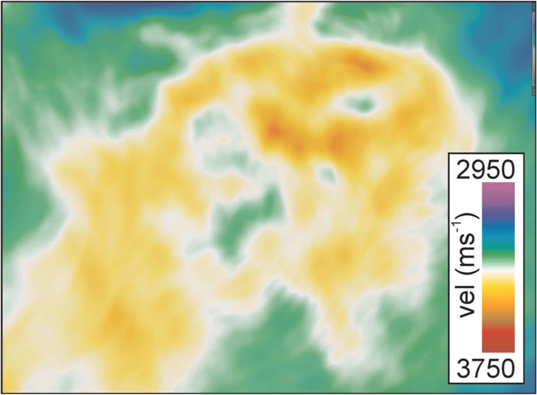
(a) Conventional method.

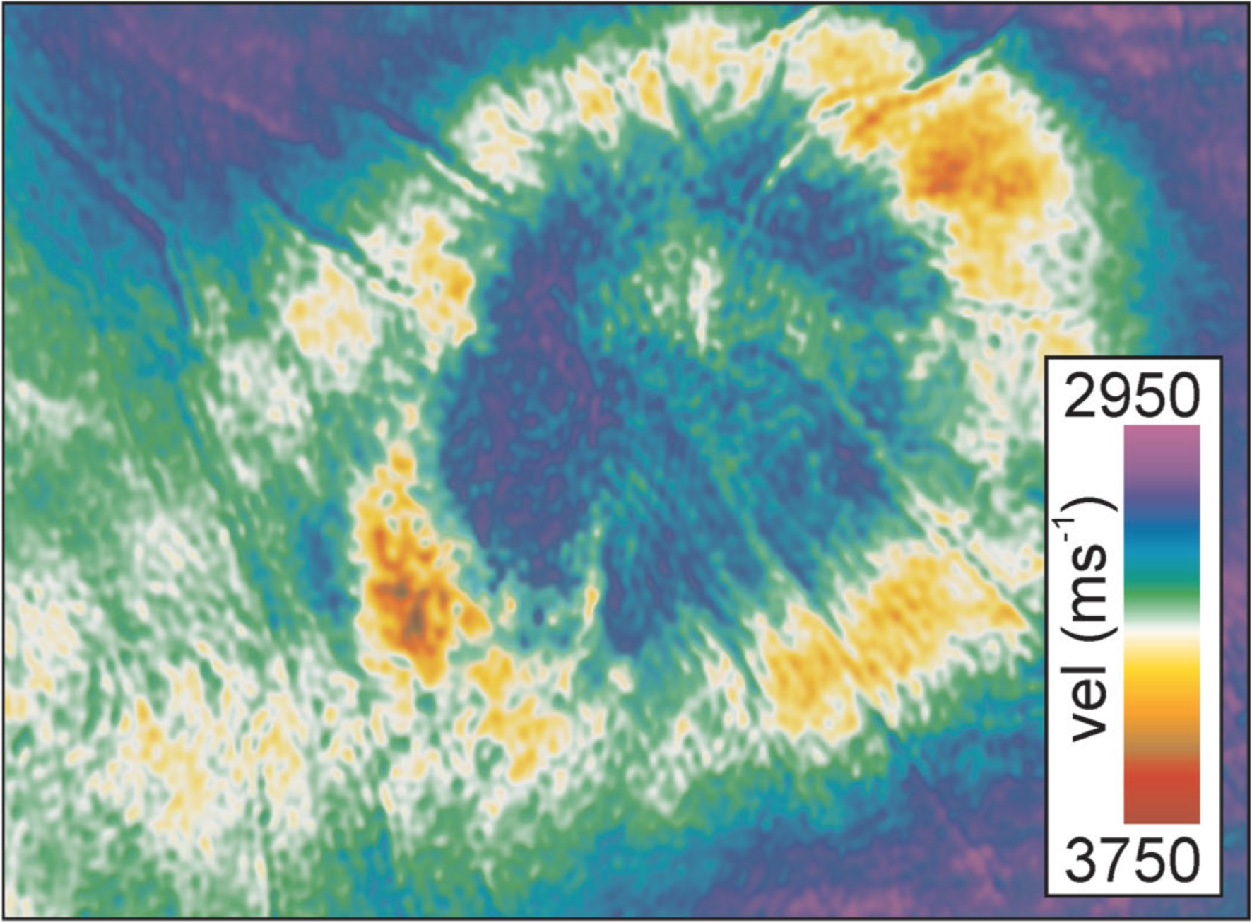
(b) $<$10Hz FWI velocity model result.

Figure 2: Horizontal slices though the Samson Dome at 1350m. From Morgan et al. [2013].

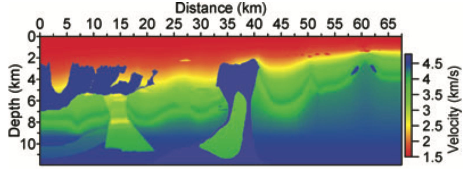
(a) Original 2004 BP synthetic for FWI.

(b) Zoomed section.

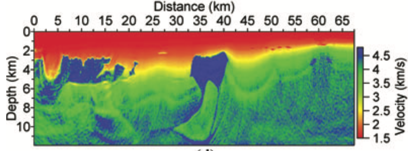
(c) 2D FWI result.

(d) Lack of resolution.

Figure 3: Limitations of FWI in complicated geology. From Shin et al. [2010].

1.2 Aims & Objectives

Optimization theory is fundamental to FWI. The parameters of the system under investigation are reconstructed from indirect observations that are subject to a forward modelling process Tarantola [2005]. The accuracy of this forward modelling depends on the validity of physical theory that links ground-truth to the measured data Innanen [2014]. Moreover, solving for this inverse problem involves learning the inverse mapping from measurements to the ground-truth which is based on a subset of degraded best-estimated data Tarantola [2005], Tikhonov and Arsenin [1977]. Two limitations within inverse theory can be identified: (i) solving the forward problem and (ii) training the data.

Choice of the numerical method used to solve the forward problem will crucially impact the accuracy of the FWI result. Challenging environments require more complex assumptions to explain the physical link between data and observations, with not necessarily improved levels of accuracies Morgan et al. [2013]. Secondly, the data being used to reconstruct the mapping of measurements for the ground-truth are not optimal. Very wide angle and multi-azimuth data are required to enable full inversion Morgan et al. [2016]; this information might not necessarily have been recorded in the acquisition stages of the data. Furthermore, pre-conditioning of data is a necessity prior to FWI to induce well-posedness Kumar et al. [2012], Mothi et al. [2013], Peng et al. [2018], Warner et al. [2013]. However, if done incorrectly this can degrade the inversion process Lines [2014]. Indeed, Lines [2014] shows how FWI remains robust to both random and coherent noise, and his work indicates that FWI with the inclusion of multiple data proves useful at estimating a better solution in some situations.

Recently, deep learning (DL) techniques have emerged as excellent models and gained great popularity for their widespread success in pattern recognition Ciresan et al. [2012, 2011], speech recognition Hinton et al. [2012] and computer vision Krizhevsky et al. [2015], Deng and Yu [2013]. The use of Deep Neural Networks (DNN) to solve inverse problems has been explored by Elshafiey [1991], Adler and Öktem [2017], Chang et al. [2017], Wei et al. [2017] and has achieved state-of-the-art performance in image reconstruction Kelly et al. [2017], Petersen et al. [2017], Adler et al. [2017], super-resolution Bruna et al. [2015], Galliani et al. [2017] and automatic-colorization Larsson et al. [2016].

In Geophysics, the applications of DL techniques have focused on the identification of features and attributes in migrated seismic sections, with few studies looking into velocity inversion. Zhang et al. [2014] used a kernel regularized least-squares method for fault detection from seismic records on numerical experiments. Wang et al. [2018] employed a fully convolutional neural network (FCN) to perform salt-detection from raw multi-shot gathers which was found to be much faster and efficient than traditional migration and interpretation. Lewis and Vigh [2017] combined DL and FWI to improve the performance for salt inversion by generating a probability map from learned abstractions of the data and incorporating these in the FWI objective function. These tests results showed promise for automated salt body reconstruction using FWI. Mosser et al. [2018] used a generative adversarial network Goodfellow et al. [2016] with cycle-constraints to perform seismic inversion by reformulating the inversion problem as a domain-transfer problem. The mapping between post-stack seismic traces and p-wave velocity models was approximated through DL. More recently, Yang and Ma [2019] developed a supervised FCN for velocity-model building directly from raw seismograms using a DNN architecture based on U-Net Ronneberger et al. [2015]. Their training data was obtained from modelling of the acoustic wave equation via a time-domain staggered-grid finite-difference scheme, with numerical experiments showing good potential of DL for seismic velocity inversion.

In this work, we are re-casting the mathematical formulation of FWI within a DL framework. The conventional least-squares formulation of FWI can be expressed as:

$$\min_{\mathbf{m}}\emph{J}(\mathbf{m})={\left||\mathbf{d}-F(\mathbf{m})\right||}_{2}^{2},$$ (1)

where $\mathbf{m}\in M$ is the subsurface model, $F:M\rightarrow D$ is the forward wave equation model, and $\mathbf{d}\in D$ is the observed data. This inversion is non-linear and ill-posed since $\mathbf{d}$ does not contain all subsurface information to define a velocity model explicitly Biondi [2006]. Based on the Universal Approximation Theorem Hornik et al. [1989], a DNN can be used to approximate the non-linear inverse operator $F^{-1}:D\rightarrow M$ by a pseudo-inverse operator or mapping function $g_{\theta}$ which minimizes the functional:

$$\emph{J}(\mathbf{m})={\left||\mathbf{m}-g_{\theta}(\mathbf{d})\right||}^{2},$$ (2)

where $\theta$ is a large simulated dataset of pairs $(\mathbf{m},\mathbf{d})$ used for learning the process function $g_{\theta}$ Hastie et al. [2001]. In particular, based on the work of Falsaperla et al. [1996], DNN utilizing pseudo-spectral transformed data $\mathcal{F}$ facilitates the learning process due to better sparsity in the transformed domain, as compared to the time domain. The novelty of this approach is the combination of both DL, signal processing and inverse theory for subsurface velocity inversion. This papers aims to prove what theory indicates is a potentially viable solution via a practical implementation to a 1D synthetic model.

The structure of this manuscript is as follows. Section 1 introduces the subject of FWI and its importance within current workflows for seismic exploration. Limitations within the current formulation are identified and a novel approach to devise better velocity models of the subsurface is proposed. In Section 2, mathematical fundamentals for FWI and DNN are derived respectively. These are then compared and their differences are highlighted. In particular, FWI is recast as a DL problem. Based on the derived formulation in Section 2, numerical results of this novel approach are presented in Section 3 and a 1D synthetic highlights the successfulness and failures of this approach. In Section 4, concluding remarks are presented.

2 Theoretical framework and methodology

2.1 Inverse problem formulation

The aim of inversion is to estimate the parameters of a physical system based on the measurements available. In the case of Geophysics, the physical system is the Earth and data are the recorded wave-field.

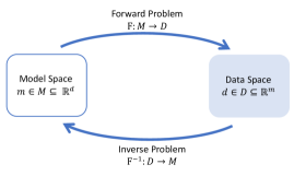
Figure 4: Visual representation of the mapping between the Forward and the Inverse problem.

The recorded wave-field is known, while the physical properties of the medium which the wave-field propagated through are the unknowns. The wave-field will be a function of these medium properties and the function for the forward problem can be as expressed as:

$$\mathbf{d}=F(\mathbf{m}),$$ (3)

where $F:M\rightarrow D,F\in\mathbb{R}^{(m\times d)}$ is the operator applied on the model space $\mathbf{m}\in M\subseteq\mathbb{R}^{d}$ to recover measurements $\mathbf{d}\in D\subseteq\mathbb{R}^{m}$. The forward problem is well-posed, that is, a unique solution exists that depends continuously on the model in some appropriate topology.

The opposite to forward modelling is the inversion. This involves making assumptions on the physical properties of the object we want to image to be able to compute the wave-field at any given time and location to a certain degree of accuracy. If $F$ is invertible, the inverse problem is given by:

$$\mathbf{m}=F^{-1}(\mathbf{d}),$$ (4)

This aims to extract all the information contained within the data.

2.2 FWI as local optimisation

Lailly [1983] and Tarantola [1984] re-cast the migration imaging principle introduced by Claerbout [1971] as a local optimisation problem. The forward problem is based on the wave equation, which is one of the most fundamental equations in Physics used for the description of wave motion. It is a second order, partial differential equation involving both time and space derivatives.

The particle motion for an isotropic medium is given by:

$$\frac{1}{c(\mathbf{m})^{2}}\frac{\partial^{2}p(\mathbf{m},t)}{\partial t^{2}}-\nabla^{2}p(\mathbf{m},t)=s(\mathbf{m},t),$$ (5)

where $p(\mathbf{m},t)$ is the pressure wave-field, $c(\mathbf{m})$ is the acoustic $p$-wave velocity and $s(\mathbf{m},t)$ is the source Igel [2016]. To solve the wave equation numerically, it can be expressed as a linear operator. Although the data $\mathbf{d}$ and model $\mathbf{m}$ are not linearly related, the wave-field $p(\mathbf{m},t)$ and the sources $s(\mathbf{m},t)$ are linearly related by the equation:

$$\mathbf{A}p(\mathbf{m},t)=s(\mathbf{m},t),$$ (6)

where $p(\mathbf{m},t)$ is the pressure wave-field produced by a source $s(\mathbf{m})$ and $\mathbf{A}$ is the numerical implementation of the operator:

$$\frac{1}{c(\mathbf{m})^{2}}\frac{\partial^{2}}{\partial t^{2}}-\nabla^{2},$$ (7)

A common technique employed within the forward modelling stage is to perform modelling in pseudo-spectral domain ($\mathcal{F}$) rather than the time domain ($\mathcal{T}$). The most common domain is the Fourier domain Igel [2016] and computational implementation is generally achieved via the Fast Fourier Transform (FFT) developed by Cooley and Tukey [1965] as it utilises the fact that $e^{-2\pi i/N}$ is an $N$-th primitive root of unity and allows for the reduction of computational costs from $O(N^{2})$ to $O(N\log N)$.

After forward modelling the data in pseudo-spectral domain, the objective is to seek to minimize the difference between the observed data and the modelled data. The metric for the difference or misfit between the two datasets is known as the misfit-, objective- or cost-function J. The most common cost function is given by the $L_{2}$-norm of the data residuals:

$$\emph{J}(\mathbf{m})=\frac{1}{2}{\left||d-F(\mathbf{m})\right||}^{2}_{D},$$ (8)

where $D$ indicates the data domain given by $n_{s}$ sources and $n_{r}$ receivers Igel [2016]. The misfit function J can be minimized with respect to the model parameters $d$ if the gradient is zero, namely:

$$\nabla\emph{J}=\frac{\partial\emph{J}}{\partial\mathbf{d}}=0,$$ (9)

Minimising the misfit function is generally achieved via a linearised iterative optimisation scheme based on the Born approximation in scattering theory Born [1980], Clayton and Stolt [1980]. The inversion algorithm starts with an initial estimate of the model $\mathbf{m}_{0}$. After the first pass via forward modelling, the model is updated by the model parameter perturbation $\Delta\mathbf{m}_{0}$. This newly updated model is then used to calculate the next update and the procedure continues iteratively until the computed model is close enough to the observations based on a residual threshold criterion. At each iteration $k$, the misfit function $\emph{J}(\mathbf{m}_{k})$ is calculated from the previous iteration model $\mathbf{m}_{k-1}$ by:

$$\emph{J}(\mathbf{m}_{k})=\emph{J}(\mathbf{m}_{k-1}+\Delta\mathbf{m}_{0}),$$ (10)

Assuming that the model perturbation is small enough with respect to the model, equation (10) can be expanded via Taylor series up to second orders as:

$$\begin{split}\emph{J}(\mathbf{m}_{k})&=\emph{J}(\mathbf{m}_{k-1}+\Delta\mathbf{m}_{0})\\ &=\emph{J}(\mathbf{m}_{k-1})+\delta\mathbf{m}^{T}_{k-1}\frac{\partial\emph{J}}{\partial\mathbf{m}_{k-1}}+\frac{1}{2}\delta\mathbf{m}^{2T}_{k-1}\frac{\partial^{2}\emph{J}}{\partial\mathbf{m}^{2}_{k-1}},\end{split}$$ (11)

Taking the derivative of equation (11) and minimizing to determine the model update leads to:

$$\delta\mathbf{m}_{k-1}\approx-\mathbf{H}^{-1}\nabla_{\mathbf{m}_{k-1}}\emph{J},$$ (12)

where $\mathbf{H}=\frac{\partial^{2}\emph{J}}{\partial\mathbf{m}^{2}_{k-1}}$ is the Hessian matrix and $\nabla_{\mathbf{m}_{k-1}}\emph{J}$ the gradient of the misfit function. The Hessian matrix is a symmetric matrix of size $N\times N$ where $N$ is the number of model parameters and represents the curvature trend of the quadratic misfit function.

FWI is an ill-posed problem, implying there exist an infinite number of models that fit the observations. Well-posedness can be introduced with the addition of Tikhonov $L_{2}$-norm regularization Tikhonov [1963], Tikhonov and Arsenin [1977]:

$$\emph{J}(\mathbf{m})=\frac{1}{2}\left[{\left||d-F(\mathbf{m})\right||}^{2}_{D}+\lambda\left||\mathbf{m}\right||^{2}_{M}\right],$$ (13)

where $\lambda$ is the regularization parameter which signifies the trade-off between the data and model residuals.

2.3 FWI algorithm summary

A summary of FWI as a local optimisation problem is given in Algorithm 1 and a schematic is illustrated in Figure 5.

Algorithm 1 FWI as a local optimisation problem

1. Choose an initial model $\mathbf{m}_{0}$ and source wavelet $s(\mathbf{m})$.

2. For each source location, solve the forward problem $F:M\rightarrow D$ using pseudo-spectral forward modelling everywhere in the model space to get a predicted wave-field $\mathbf{d}_{k}$. This is sampled at receivers $r(\mathbf{m})$.

3. At every receiver $r(\mathbf{m})$, data residuals are calculated between the modelled wave-field $\mathbf{d}_{k}$ and the observed data $\mathbf{d}$.

4. These data residuals are back-propagated from the receivers to produce a back-propagated residual wave-field.

5. For each source location, the misfit function $\emph{J}(\mathbf{m})$ is calculated for the observed data and back-propagated residual wave-field to generate the gradient $\nabla\emph{J}$ required at every point in the model.

6. The gradient is scaled based on the step-length $\alpha$, applied to the starting model and an updated model is obtained $\mathbf{m}_{(k+1)}$.

7. The process is iteratively repeated from Step 2 until the convergence criterion is satisfied.

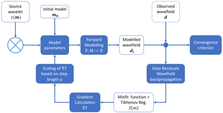
Figure 5: Schematic of a FWI workflow solved as an iterative optimisation process.

2.4 Deep Neural Networks for FWI

Neural Networks (NN) are a subset of tools in machine learning which when applied to inverse problems can approximate the non-linear functional of the inverse problem $F^{-1}:D\rightarrow M$. That is, using a NN, a non-linear mapping can be learned to minimize

$$\left||\mathbf{m}-g_{\theta}(\mathbf{d})\right||^{2},$$ (14)

where $\theta$ the large data set of pairs $(\mathbf{m},\mathbf{d})$ used for the learning process Lucas et al. [2018].

The most elementary component in a NN is a neuron. This receives excitatory input and sums the result to produce an output or activation, representing a neuron’s action potential which is transmitted along its axon Raschka and Mirjalili [2017]. For a given artificial neuron, consider $n$ inputs with signals $m$ and weights $w$. The output $d$ of the $k^{\text{th}}$ neuron from all input signals is given by:

$$d_{k}=\sigma\left(b+\sum_{j=0}^{m}w_{kj}m_{j}\right),$$ (15)

where $\sigma$ is the activation function and $b$ is a bias term enabling the activation functions to shift about the origin.

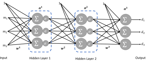
Figure 6: An example of a fully connected NN with 2 hidden layers. All weights $w$ and bias $b$ are learned during the training phase. The $1$’s connected to each hidden layer represents bias nodes which help the NN learn patterns by allowing the output of an activation function to be shifted. Adapted from Lucas et al. [2018].

When multiple neurons are combined together, they form a NN. The architecture of a NN refers to the number of neurons, their arrangement and their connectivity Šíma and Orponen [2003]. The initial layer of nodes $\mathbf{m}$ are referred to as the Input Layer. These are connected to a sequence of hidden layers of neurons. The final layer of the neurons is not a hidden layer and is referred to as the Output Layer. Communication proceeds layer by layer from the input layer via the hidden layers up to the output layer. If a NN has two or more hidden layers, it is called a DNN. Figure 6 shows a NN consisting of 2 hidden layers. The output of the unit in each layer is the result of the weighted sum of the input units, followed by a non-linear element-wise function. The weights between each units are learned as a result of a training procedure.

When training a DNN, the forward propagation through the hidden layers from input $\mathbf{m}$ to output $\mathbf{d}$ needs to be measured for its misfit. The most commonly used cost function is the Sum of Squared Errors (SSE), defined as:

$$\emph{J}(\mathbf{m})=\frac{1}{2}\sum_{i=1}^{J}\left(\mathbf{m}-g_{\theta}(\mathbf{d}^{(i)})\right)^{2},$$ (16)

where $\mathbf{d}$ is the labelled true dataset, $\mathbf{d}^{(i)}$ is the output from the $i^{\text{th}}$ forward pass through the network and the summation is across all neurons in the network. The objective is to minimize the function J with respect to the weights $w$ of the neurons in the NN. Employing the Chain Rule and after a series of recursive formulations, the error signals for all neurons in the network can be recursively calculated throughout the network and the derivative of the cost function with respect to all the weights $w$ can be calculated. Training of the DNN is then achieved via a Gradient Descent algorithm, referred to as back-propagation training algorithm Rumelhart et al. [1985]. The reader is referred to Goodfellow et al. [2016] and citations therein for a full mathematical formulation.

2.5 Outline for solving FWI using DNN

Algorithm for training of a DNN for FWI is given in Algorithm 2 and a schematic is given in Figure 7.

Algorithm 2 FWI as a DNN problem

1. Setup a deep architecture for the NN.

2. Initialise the set of weights $w^{l}$ and biases $b^{l}$.

3. Forward propagate through the network connections to calculate input sums and activation function for all neurons and layers.

4. Calculate the error signal for the final layer $\delta^{L}$ by choosing an appropriate differentiable activation function.

5. Back-propagate the errors $(\delta^{l})$ for all neurons in layer $l$.

6. Differentiate the cost function with respect to biases $\left(\frac{\partial\emph{J}}{\partial b^{l}}\right)$.

7. Differentiate the cost function with respect to weights $\left(\frac{\partial\emph{J}}{\partial w^{l}}\right)$.

8. Update weights $w^{l}$ via gradient descent.

9. Recursively repeat from Step 3 until the desired convergence criterion is met.

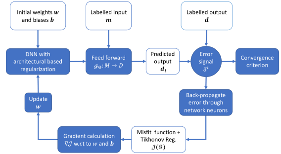
Figure 7: Schematic of a FWI workflow solved as learned optimisation process.

3 Numerical example

3.1 Experiment setup

The hypothesis we would like to prove is as follows:

"Given a seismic trace in time domain, invert for the seismic velocity ($v_{p}$) via a DNN which transforms the input data into pseudo-spectral domain and learns to invert for a velocity estimate"

3.2 Training data

Learning of the inversion from time to pseudo-spectral domain requires a training dataset which maps time to Fourier components of magnitude and phase, and their respective velocity profile. For our numeric example, 500,000 randomly generated mappings from time $(\mathcal{T})$ to Fourier components $(\mathcal{F})$ for a 2000ms time window were created. The steps involved in creation of the synthetic are shown in Figure 8 for a sample velocity profile and the steps involved in creating the dataset are given as:

1. Randomly create a $v_{p}$ velocity profile for a $2000ms$ time duration, with values ranging from $1400ms^{-1}$ to $4000ms^{-1}$. The lower bound of $1400ms^{-1}$ was selected as in normal off-shore seismic exploration conditions, the smallest observed velocity is that of the water which ranges from $1450ms^{-1}$ to $1460ms^{-1}$ Cochrane and Cooper [1991]. The upper bound of $4000ms^{-1}$ was selected as this is the upper limit of velocity in porous and saturated sandstones Lee et al. [1996] and the assumption is made that limestones, carbonates and salt deposits are not present in the subsurface model being inverted as these have velocity ranges in excess of $4000ms^{-1}$.

2. Calculate the density $\rho$ based on Gardner’s equation Gardner et al. [1974] given by $\rho=\alpha v_{p}^{\beta}$ where $\alpha=0.31$ and $\beta=0.25$ are empirically derived constants that depend on the Geology.

3. At each interface, calculate the Reflection Coefficient $\mathcal{R}=\frac{\rho_{2}v_{p_{2}}-\rho_{1}v_{p_{1}}}{\rho_{2}v_{p_{2}}+\rho_{1}v_{p_{1}}}$ where $\rho_{i}$ is density of medium $i$ and $v_{p_{i}}$ is the $p$-velocity in medium $i$

4. For each medium, calculate the Acoustic Impedance $\mathcal{Z}_{i}=\rho_{i}v_{p_{i}}$

5. Define a wavelet $\mathcal{W}$. This was selected to be a Ricker wavelet at 10$\mathrm{H}\mathrm{z}$ Ricker [1943]. The Ricker wavelet is a theoretical waveform that takes into account the effect of Newtonian viscosity and is representative of seismic waves propagating through visco-elastic homogeneous media Wang [2015], thus making it ideal for this numerical simulation. The central frequency of 10$\mathrm{H}\mathrm{z}$ was chosen as a nominal value based on literature results to be representative of normal FWI conditions Morgan et al. [2013]. Beyond 10$\mathrm{H}\mathrm{z}$ would be considered to be super-high-resolution FWI Mispel et al. [2019], which goes beyond the scope of this manuscript.

6. The Reflection Coefficient and wavelet are convolved to produce the seismic trace $\mathcal{T}$

7. Fourier coefficients for magnitude $\mathcal{F}(\zeta)$ and phase $\mathcal{F}(\phi)$ are derived based on the FFT.

Figure 8: Workflow for creating a pseudo-spectral synthetic trace. This was repeated 500,000 times with random parameters generated within the pre-defined limits stated in Section 3.2 to create the learning dataset.

3.3 DNN architecture

Figure 9 illustrates the NN architecture used to first invert for the Fourier coefficients from the time domain and then invert for velocity profile. The complete workflow had 5 modules, with each module consisting of NN with 5 fully-connected hidden layers. The layer distributions consisted of an input layer of 2000 neurons, then a set of 5 hidden layers of sizes 1000, 500, 250, 500, 1000 neurons, and an output layer of 2000 neurons. This hour-glass design can be considered representative of multi-scale FWI Bunks et al. [1995] since at each hidden layer, the NN learns an abstracted component of the data at a different scale. The network employed a sum of squared errors loss function, data batching, early stopping, $L_{2}$ - norm regularization updates and executed for 200 epochs. A Rectified linear unit or ReLU function given by $f(x)=\max(0,x)$ was used as an activation function. This is a non-linear function which allows for back-propagation of errors. When employed on a network of neurons, the negative component of the function is converted to zero and the neuron is deactivated, thus introducing sparsity within the network and making it efficient and easy for computation. The output from each parallel thread in the flow is fed into another neural network which learns the optimal way of combining the outputs. In total, the DNN had 25 hidden layers. The learning or back-propagation for each network was optimized via an ADAM optimizer Kingma and Ba [2014], which is a stochastic gradient descent based algorithm for first-order gradient-based optimisation which employs on adaptive estimates of lower-order moments. The DNN was implemented in Python 3.7, using Keras 2.2.4 Chollet et al. [2015] and TensorFlow 1.13.1 Abadi et al. [2016] backend.

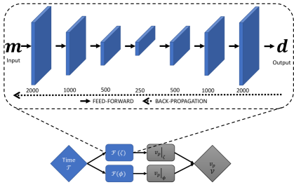
Figure 9: Pseudo-spectral FWI DNN architecture. The highlighted section indicates the set-up employed in each of the 5 modules. Each network has an hour-glass shape with layers of sizes 2000-1000-500-250-500-1000-2000 neuron which can be related to multi-scale FWI. The bottom section illustrates the DNN workflow where $\mathcal{T}$ is the input time domain, $\mathcal{V}$ is the output $v_{p}$ velocity and $\mathcal{F}$ is the Fourier domain, with magnitude $\zeta$ and phase $\phi$.

3.4 Numerical results

Figure 10: Four different predictions obtained from learned weights of the DNN on unseen data. The top panels are the velocity profile reconstructions from the two NN architecture branches ($\mathcal{F}(\zeta)$ and $\mathcal{F}(\phi)$) and the combined result. Bottom panels are the observed and inverted waveforms.

(a) Training dataset MSE over the different epochs per DNN component. Overall performance is decreasing per epoch, indicating that the DNN is learning to invert.

(b) Test dataset MSE over the different epochs per DNN component.

(c) Learning Rate performance over the different epochs per DNN component.

Figure 11: DNN performance metrics.

Figure 10 illustrates the application of DNN architecture in Section 3.3 for a sample of unseen data and the respective reconstruction. Inspection of the first 750$\mathrm{m}\mathrm{s}$ indicates that the DNN approach is able to reconstruct both the velocity and the waveform profile near perfectly, irrespective of the number of layers and the magnitude of the acoustic difference in this time range. Beyond 750$\mathrm{m}\mathrm{s}$, reconstructions start suffering from slight degradation. As illustrated in the velocity reconstruction of the middle figure, the inaccuracy is minimal and ranges $\pm$100$\mathrm{m}\mathrm{s}^{-1}$. However, this leads to perturbations in the reconstruction and does not allow for perfect matching. Further inspection suggests that the main source of error is due to the magnitude component of the network (red). To improve this error component, the network inverting for the magnitude component of the FFT would need to be trained and generalised further.

Figure 11 shows the DNN metric performance over the different epochs per DNN component. Figure 11(a) and 11(b) illustrate the MSE performance for the training and testing dataset respectively. Considering the former, the plots indicate that the network is indeed learning since MSE is decreasing at each epoch. Comparing respective DNN components between the training and the testing dataset metrics, there is evidence of no under-fitting or over-fitting with the pseudo-spectral learning components of the DNN architecture (net_time_mag, net_mag_vels, net_time_phase, net_phase_vel) and there is indeed good-fit since training and testing MSE both decrease to a point of stability with a minimal difference between the two final MSE values. On the other hand, net_avg_vel component which is learning to average out the velocity from Fourier components indicates symptoms of an under-presented training dataset. Moreover, these MSE performance plots indicate that the technique might suffer from a compounding error issue. The two best performing components are the first layer of learning for the inversion, namely Time-to-FFT-Magnitude (net_time_mag) and Time-to-FFT-Phase (net_time_phase), as their MSE performance plateaus at $10^{-1}$. In the second phase of the inversion which converts respective FFT components to velocities (FFT-Magnitute-to-Velocity (net_mag_vels) and FFT-Phase-to-Velocity (net_phase_vels)), the error plateaus are at $10^{1}$, which is two orders of magnitude greater. The final network component sits even higher on the scale at $10^{2}$. Both the train and the test dataset show drastic decreases in the MSE at different epoch levels. These can be attributed to the step-wise reductions in learning rate shown in Figure 11(c). This varying learning rate allows the network to move to a deeper optimisation level and approach a more global minima for the optimisation problem.

4 Conclusions

In this manuscript we presented the investigation of direct modelling for seismic waveforms using a DNN which first converts data to pseudo-spectral domain and inverts for velocity profiles. Experimental results demonstrated that the use of synthetically generated data to train a DNN proves to be a viable technique to learn how to invert via pseudo-spectral data. Although inversion was successfully achieved in the numerical examples presented, one branch of the DNN architecture was lacking in inversion performance and was resulting in a compounding error effect. To improve the overall performance of the technique, data augmentation will be considered as potentially 500,000 random traces are not sufficient to train the magnitude component of the Fourier transform for the network to achieve a desirable performance, and fine-tuning of the NN architecture in the form of in-between layer regularization, neuron drop-out during epoch training and convolutional layers have yet to be investigated. Moreover, in the next stage, this technique will be used for the inversion of more interesting subsurface structures which have a geological relevance, evaluate image resolution when compared to standard FWI and also consider the case of a sequential input in the form of a Recurrent Neural Network, similar to the work of Sun et al. [2019], but via a pseudo-spectral approach.

References

- Abadi et al. [2016] Martín Abadi, Ashish Agarwal, Paul Barham, Eugene Brevdo, Zhifeng Chen, Craig Citro, Greg S Corrado, Andy Davis, Jeffrey Dean, Matthieu Devin, et al. Tensorflow: Large-scale machine learning on heterogeneous distributed systems. arXiv preprint arXiv:1603.04467, 2016.
- Adler and Öktem [2017] Jonas Adler and Ozan Öktem. Solving ill-posed inverse problems using iterative deep neural networks. Inverse Problems, 33(12):1–24, 12 2017. ISSN 0266-5611. doi: 10.1088/1361-6420/aa9581.
- Adler et al. [2017] Jonas Adler, Axel Ringh, Ozan Öktem, and Johan Karlsson. Learning to solve inverse problems using Wasserstein loss. Iclr 2018, pages 1–13, 2017. URL http://arxiv.org/abs/1710.10898.
- Biondi [2006] Biondo L Biondi. 3D seismic imaging. Society of Exploration Geophysicists, 2006.
- Born [1980] Max Born. E. Wolf Principles of optics. Pergamon Press, 6:188–189, 1980.
- Bruna et al. [2015] Joan Bruna, Pablo Sprechmann, and Yann LeCun. Super-Resolution with Deep Convolutional Sufficient Statistics. 11 2015. URL http://arxiv.org/abs/1511.05666.
- Bunks et al. [1995] Carey Bunks, Fatimetou M Saleck, S Zaleski, and G Chavent. Multiscale seismic waveform inversion. Geophysics, 60(5):1457–1473, 1995. ISSN 0016-8033.
- Chang et al. [2017] J H Chang, Chun-Liang Li, Barnabás Póczos, B V K Kumar, and Aswin C Sankaranarayanan. One Network to Solve Them All—Solving Linear Inverse Problems using Deep Projection Models. IEEE International Conference on Computer Vision (ICCV), 2017. doi: 10.1109/ICCV.2017.627. URL http://openaccess.thecvf.com/content{_}ICCV{_}2017/papers/Chang{_}One{_}Network{_}to{_}ICCV{_}2017{_}paper.pdf.
- Chollet et al. [2015] François Chollet et al. Keras. https://keras.io, 2015.
- Ciresan et al. [2012] Dan Ciresan, Ueli Meier, Jonathan Masci, and Jürgen Schmidhuber. Multi-column deep neural network for traffic sign classification. Neural networks, 32:333–338, 2012.
- Ciresan et al. [2011] Dan C Ciresan, Ueli Meier, Jonathan Masci, and Jürgen Schmidhuber. A committee of neural networks for traffic sign classification. pages 1918–1921, 2011.
- Claerbout [1971] J Claerbout. Toward a unified theoru of relector mapping. Geophysics, 36(June), 1971.
- Clayton and Stolt [1980] Robert W Clayton and Robert Stolt. A Born-WKBJ Inversion Method for Acoustic Reflection Data. In SEP-Report, volume 46, pages 135–158. 1980.
- Cochrane and Cooper [1991] Guy Cochrane and A.K. Cooper. Sonobuoy seismic studies at odp drill sites in prydz bay, antarctica. pages 27–43, 01 1991.
- Cooley and Tukey [1965] James W Cooley and John W Tukey. An algorithm for the machine calculation of complex fourier series. Mathematics of computation, 19(90):297–301, 1965.
- Deng and Yu [2013] Li Deng and Dong Yu. Deep Learning: Methods and Applications. Foundations and Trends® in Signal Processing, 2013. ISSN 09598138. doi: 10.1136/bmj.319.7209.0a. URL http://www.nowpublishers.com/article/Details/SIG-039.
- Elshafiey [1991] Ibrahim Mohamed Elshafiey. Neural network approach for solving inverse problems. 1991.
- Falsaperla et al. [1996] S. Falsaperla, S. Graziani, G. Nunnari, and S. Spampinato. Automatic classification of volcanic earthquakes by using multi-layered neural networks. Natural Hazards, 13(3):205–228, 1996. ISSN 0921030X. doi: 10.1007/BF00215816.
- Galliani et al. [2017] Silvano Galliani, Charis Lanaras, Dimitrios Marmanis, Emmanuel Baltsavias, and Konrad Schindler. Learned Spectral Super-Resolution. 2 2017. URL http://arxiv.org/abs/1703.09470.
- Gardner et al. [1974] G. H. F. Gardner, L. W. Gardner, and A. R. Gregory. Formation Velocity and Density - The diagnostic basics for Stratigraphic Traps. GEOPHYSICS, 39(6):770–780, 12 1974. ISSN 0016-8033. doi: 10.1190/1.1440465. URL http://library.seg.org/doi/10.1190/1.1440465.
- Goodfellow et al. [2016] Ian Goodfellow, Yoshua Bengio, and Aaron Courville. Deep Learning. MIT Press, 2016. http://www.deeplearningbook.org.
- Hastie et al. [2001] Trevor Hastie, Jerome Friedman, and Robert Tibshirani. The Elements of Statistical Learning. Springer Series in Statistics, 2001. ISSN 0172-7397. doi: 10.1007/978-0-387-21606-5.
- Hinton et al. [2012] Geoffrey Hinton, Li Deng, Dong Yu, George E Dahl, Abdel-rahman Mohamed, Navdeep Jaitly, Andrew Senior, Vincent Vanhoucke, Patrick Nguyen, and Tara N Sainath. Deep neural networks for acoustic modeling in speech recognition: The shared views of four research groups. IEEE Signal processing magazine, 29(6):82–97, 2012. ISSN 1053-5888.
- Hornik et al. [1989] K Hornik, M Stinchcombe, and H White. Multilayer feedforward networks are universal approximator. Neural Networks, 2:359–366, 1989. ISSN 08936080. doi: 0893-6080/89.
- Igel [2016] Heiner Igel. Computational Seismology. 2016. doi: 10.1093/acprof:oso/9780198717409.001.0001. URL http://www.oxfordscholarship.com/view/10.1093/acprof:oso/9780198717409.001.0001/acprof-9780198717409.
- Innanen [2014] Kris Innanen. Quantifying the incompleteness of the physics model in seismic inversion. CREWES Research Report, 2014.
- Kelly et al. [2017] Brendan Kelly, Thomas P Matthews, and Mark A Anastasio. Deep Learning-Guided Image Reconstruction from Incomplete Data. (Nips), 2017. URL http://arxiv.org/abs/1709.00584.
- Kingma and Ba [2014] Diederik P Kingma and Jimmy Ba. Adam: A method for stochastic optimization. arXiv preprint arXiv:1412.6980, 2014.
- Krizhevsky et al. [2015] Alex Krizhevsky, Ilya Sutskever, Geoffrey E. Hinton, Tugce Tasci, and Kyunghee Kim. ImageNet Classification with Deep Convolutional Neural Networks. Stanford cs231b, 2015. URL http://vision.stanford.edu/teaching/cs231b{_}spring1415/slides/alexnet{_}tugce{_}kyunghee.pdf.
- Kumar et al. [2012] J Kumar, AC Ramrez, and S Butt. Preparing Data for Full Waveform Inversion: A Workflow for Free-surface Multiple Attenuation. 74th EAGE Conference and Exhibition-Workshops, 2012. URL http://www.earthdoc.org/publication/publicationdetails/?publication=59914.
- Lailly [1983] Patrick Lailly. The seismic inverse problem as a sequence of before stack migrations. 1983.
- Lailly and Bednar [1983] Patrick Lailly and JB Bednar. The seismic inverse problem as a sequence of before stack migrations. In Conference on inverse scattering: theory and application, pages 206–220. Siam Philadelphia, PA, 1983.
- Larsson et al. [2016] Gustav Larsson, Michael Maire, and Gregory Shakhnarovich. Learning representations for automatic colorization. In Lecture Notes in Computer Science (including subseries Lecture Notes in Artificial Intelligence and Lecture Notes in Bioinformatics), volume 9908 LNCS, pages 577–593, 2016. ISBN 9783319464923. doi: 10.1007/978-3-319-46493-0_35. URL http://link.springer.com/10.1007/978-3-319-46493-0{_}35.
- Lee et al. [1996] MW Lee, DR Hutchinson, TS Collett, and William P Dillon. Seismic velocities for hydrate-bearing sediments using weighted equation. Journal of Geophysical Research: Solid Earth, 101(B9):20347–20358, 1996.
- Lewis and Vigh [2017] Winston Lewis and Denes Vigh. Deep learning prior models from seismic images for full-waveform inversion. In SEG Technical Program Expanded Abstracts 2017, pages 1512–1517. Society of Exploration Geophysicists, 2017.
- Lines [2014] L Lines. FWI and the "Noise" Quandary. CREWES Research Report, 2014.
- Lucas et al. [2018] Alice Lucas, Michael Iliadis, Rafael Molina, and Aggelos K. Katsaggelos. Using Deep Neural Networks for Inverse Problems in Imaging: Beyond Analytical Methods. IEEE Signal Processing Magazine, 35(1):20–36, 2018. ISSN 10535888. doi: 10.1109/MSP.2017.2760358.
- Mispel et al. [2019] J Mispel, A Furre, A Sollid, and FA Maaø. High frequency 3d fwi at sleipner: A closer look at the co2 plume. In 81st EAGE Conference and Exhibition 2019, 2019.
- Morgan et al. [2013] Joanna Morgan, Michael Warner, Rebecca Bell, Jack Ashley, Danielle Barnes, Rachel Little, Katarina Roele, and Charles Jones. Next-generation seismic experiments: wide-angle, multi-azimuth, three-dimensional, full-waveform inversion. Geophysical Journal International, 195(3):1657–1678, 2013.
- Morgan et al. [2016] Joanna Morgan, Michael Warner, Gillean Arnoux, Emilie Hooft, Douglas Toomey, Brandon VanderBeek, and William Wilcock. Next-generation seismic experiments - II: Wide-angle, multi-azimuth, 3-D, full-waveform inversion of sparse field data. Geophysical Journal International, 204(2):1342–1363, 2 2016. ISSN 1365246X. doi: 10.1093/gji/ggv513. URL https://academic.oup.com/gji/article-lookup/doi/10.1093/gji/ggv513.
- Mosser et al. [2018] Lukas Mosser, Wouter Kimman, Jesper Dramsch, Steve Purves, A De la Fuente Briceño, and Graham Ganssle. Rapid seismic domain transfer: Seismic velocity inversion and modeling using deep generative neural networks. In 80th EAGE Conference and Exhibition 2018, 2018.
- Mothi et al. [2013] Sabaresan Mothi, Katherine Schwarz, and Huifeng Zhu. Impact of full-azimuth and long-offset acquisition on Full Waveform Inversion in deep water Gulf of Mexico. SEG Houston 2013 Annual Meeting, (June 2013):924–928, 2013. ISSN 19494645. doi: 10.1190/sbgf2013-068. URL https://www.cgg.com/technicalDocuments/cggv{_}0000015203.pdf.
- Peng et al. [2018] Chao Peng, Minshen Wang, Nicolas Chazalnoel, and Adriano Gomes. Subsalt imaging improvement possibilities through a combination of FWI and reflection FWI. The Leading Edge, 37(1):52–57, 2018. ISSN 1070-485X. doi: 10.1190/tle37010052.1. URL https://doi.org/10.1190/tle37010052.1.https://library.seg.org/doi/10.1190/tle37010052.1.
- Petersen et al. [2017] Philipp C Petersen, Helmut Bölcskei, Philipp Grohs, and Gitta Kutyniok. Optimal approximation with sparse deep neural networks. 2017. URL http://anarm.dima.unige.it/genova2017/files/petersen.pdfhttp://arxiv.org/abs/1705.01714.
- Raschka and Mirjalili [2017] Sebastian Raschka and Vahid Mirjalili. Python machine learning. Packt Publishing Ltd, 2017.
- Ricker [1943] Norman Ricker. Further developments in the wavelet theory of seismogram structure. Bulletin of the Seismological Society of America, 33(3):197–228, 1943.
- Ronneberger et al. [2015] Olaf Ronneberger, Philipp Fischer, and Thomas Brox. U-net: Convolutional networks for biomedical image segmentation. In International Conference on Medical image computing and computer-assisted intervention, pages 234–241. Springer, 2015.
- Rumelhart et al. [1985] David E Rumelhart, Geoffrey E Hinton, and Ronald J Williams. Learning internal representations by error propagation. Technical report, California Univ San Diego La Jolla Inst for Cognitive Science, 1985.
- Shin et al. [2010] Changsoo Shin, Nam-Hyung Koo, Young Ho Cha, and Keun-Pil Park. Sequentially ordered single-frequency 2-d acoustic waveform inversion in the laplace–fourier domain. Geophysical Journal International, 181(2):935–950, 2010.
- Šíma and Orponen [2003] Jiří Šíma and Pekka Orponen. General-Purpose Computation with Neural Networks: A Survey of Complexity Theoretic Results, 12 2003. ISSN 08997667. URL http://www.mitpressjournals.org/doi/10.1162/089976603322518731.
- Sun et al. [2019] Jian Sun, Zhan Niu, Kristopher A Innanen, Junxiao Li, and Daniel O Trad. A theory-guided deep learning formulation of seismic waveform inversion. In SEG Technical Program Expanded Abstracts 2019, pages 2343–2347. Society of Exploration Geophysicists, 2019.
- Tarantola [1984] Albert Tarantola. Inversion of seismic reflection data in the acoustic approximation. Geophysics, 49(8):1259–1266, 1984.
- Tarantola [1987] Albert Tarantola. Inverse problems theory, methods for data fitting and model parameter estimation, 181-188, 1987.
- Tarantola [2005] Albert Tarantola. Inverse problem theory and methods for model parameter estimation, volume 89. siam, 2005.
- Tikhonov [1963] A N Tikhonov. On the Solution of Incorrectly Stated Problems and a Method of Regularization. Dokl. Acad. Nauk SSSR, 151:501–504, 1963. URL http://www.mathnet.ru/eng/dan28329.
- Tikhonov and Arsenin [1977] A N Tikhonov and Vasili Ya Arsenin. Methods for solving ill-posed problems. John Wiley and Sons, Inc, 1977.
- Virieux and Operto [2009] Jean Virieux and Stéphane Operto. An overview of full-waveform inversion in exploration geophysics. Geophysics, 74(6):WCC1–WCC26, 2009.
- Wang et al. [2018] W Wang, F Yang, and J Ma. Automatic salt detection with machine learning. In 80th EAGE Conference and Exhibition 2018, 2018.
- Wang [2015] Yanghua Wang. Frequencies of the ricker wavelet. Geophysics, 80(2):A31–A37, 2015.
- Warner et al. [2013] Michael Warner, Andrew Ratcliffe, Tenice Nangoo, Joanna Morgan, Adrian Umpleby, Nikhil Shah, Vetle Vinje, Ivan Štekl, Lluís Guasch, Caroline Win, Graham Conroy, and Alexandre Bertrand. Anisotropic 3D full-waveform inversion. GEOPHYSICS, 78(2):R59–R80, 2013. ISSN 0016-8033. doi: 10.1190/geo2012-0338.1. URL http://library.seg.org/doi/10.1190/geo2012-0338.1.
- Wei et al. [2017] Q Wei, K Fai, and L Carin. An Inner-loop Free Solution to Inverse Problems using Deep Neural Networks. Advances in Neural Information Processing Systems, pages 2370–2380, 2017. ISSN 10495258.
- Yang and Ma [2019] Fangshu Yang and Jianwei Ma. Deep-learning inversion: a next generation seismic velocity-model building method. Geophysics, 84(4):1–133, 2019.
- Zhang et al. [2014] Chiyuan Zhang, Charlie Frogner, M Araya-Polo, and D Hohl. Machine-learning based automated fault detection in seismic traces. In 76th EAGE Conference and Exhibition 2014, 2014.