Active Re-identification Attacks on Periodically Released Dynamic Social Graphs

Abstract

Active re-identification attacks pose a serious threat to privacy-preserving social graph publication. Active attackers create fake accounts to build structural patterns in social graphs which can be used to re-identify legitimate users on published anonymised graphs, even without additional background knowledge. So far, this type of attacks has only been studied in the scenario where the inherently dynamic social graph is published once. In this paper, we present the first active re-identification attack in the more realistic scenario where a dynamic social graph is periodically published. The new attack leverages tempo-structural patterns for strengthening the adversary. Through a comprehensive set of experiments on real-life and synthetic dynamic social graphs, we show that our new attack substantially outperforms the most effective static active attack in the literature by increasing the success probability of re-identification by more than two times and efficiency by almost 10 times. Moreover, unlike the static attack, our new attack is able to remain at the same level of effectiveness and efficiency as the publication process advances. We conduct a study on the factors that may thwart our new attack, which can help design graph anonymising methods with a better balance between privacy and utility.

Keywords: privacy-preserving social graph publication, re-identification attack, active adversary, dynamic social networks

1 Introduction

Social graphs have proven to be a valuable data source for conducting sociological studies, market analyses, and other forms of complex data analysis. This creates a strong incentive for the establishment of a mutually beneficial relation between analysts and data owners. For analysts, it is of paramount importance to have access to abundant, reliable social graph data in order to conduct their studies. For data owners, making these data available to third parties opens a number of additional business opportunities, as well as opportunities for improving their social perception by contributing to the advancement of research. However, releasing social network data raises serious privacy concerns, due to the sensitive nature of much of the information implicitly or explicitly contained in social graphs. Consequently, the data needs to be properly sanitised before publication.

It has been shown that some forms of sanitisation, e.g. removing users’ identities and personally identifying information from the released data, a process known as pseudonymisation, are insufficient for protecting sensitive information. This is due to the fact that a majority of users can still be unambiguously re-identified in the pseudonymised graph by means of simple structural patterns [14, 22, 2, 23]. The re-identification subsequently facilitates inferring relations between users, group affiliations, etc. A method allowing a malicious agent, or adversary, to re-identify (a subset of) the users in a sanitised social graph is called a re-identification attack.

A large number of anonymisation methods have been proposed for publishing sanitised social graphs that effectively resist re-identification attacks. The largest family of graph anonymisation methods (e.g. [14, 16, 3, 5, 33, 17, 30, 29, 4, 38, 39, 34, 18, 19]) follows a common strategy of editing the vertex and/or edge set of the pseudonymised graph in order to satisfy some formal privacy properties. These privacy properties rely on an adversary model, which encodes a number of assumptions about the adversary capabilities. In the context of social graph publication, there are two classes of adversaries. On the one hand, passive adversaries depend on publicly available information, in case that it can be obtained from online resources, public records, etc., without interacting with the social network before publication. On the other hand, active adversaries interact with the network before the sanitised dataset is released, in order to force the existence of structural patterns. Then, when the sanistised graph is published, they leverage these patterns for conducting the re-identification. Active adversaries have been shown to be a serious threat to social graph publication [2, 20], as they remain plausible even if no public background knowledge is available. Active attackers have the capability of inserting fake accounts in the social network, commonly called sybil nodes, and creating connection patterns between these fake accounts and a set of legitimate users, the victims. After the publication of the sanitised graph, the attacker uses these unique patterns for re-identifying the victims.

Social networks are inherently dynamic. Moreover, analysts require datasets containing dynamic social graphs in order to conduct numerous tasks such as community evolution analysis [6], link prediction [15] and link persistence analysis [25], among others. Despite the need for properly anonymised dynamic social graphs, the overwhelming majority of studies on graph anonymisation have focused on the scenario of a social graph being released only once. The rather small number of studies on dynamic social graph publication have provided only a partial understanding of the field, as they have exclusively focused on passive adversary models. Consequently, the manners in which active adversaries can profit from a dynamic graph publication scenario remain unknown. In this paper, we remedy this situation by formulating active re-identification attacks in the scenario of dynamic social graphs. We consider a scenario where the underlying dynamic graph is periodically sampled for snapshots, and sanitised versions of these snapshots are published. We model an active adversary whose knowledge consists in tempo-structural patterns, instead of exclusively structural patters as those used by the original (static) active adversary. Moreover, in our model the adversary knowledge is incremental, as it grows every time a new snapshot is released, and the adversary has the opportunity to adapt along the publication process. Under the new model, we devise for the first time a dynamic active re-identification attack on periodically released dynamic social graphs. The new attack is more effective than the alternative of executing independent static attacks on different snapshots. Furthermore, it is also considerably more efficient than the previous attacks, because it profits from temporal patterns to accelerate the search procedures in the basis of several of its components.

Our contributions. The main contributions of this paper are listed in what follows:

• We formulate, for the first time, active re-identification attacks in the scenario of periodically released dynamic social graphs.

• Based on the new formulation, we present, to the best of our knowledge, the first dynamic active re-identification attack on periodically released dynamic social graphs, which constructs and leverages tempo-structural patterns for re-identification.

• We conduct a comprehensive set of experiments on real-life and synthetic dynamic social graphs, which demonstrate that the dynamic active attack is more than two times more effective than the alternative of repeatedly executing the strongest active attack reported in the literature for the static scenario [20].

• Our experiments also show that, as the number of published snapshots grows, the dynamic active attack runs almost 10 times faster than the static active attack from [20].

• We analyse the factors that affect the effectiveness of our new attack. The conclusions of this study serve as a starting point for the development of anonymisation methods for the new scenario.

Structure of the paper. We discuss the related work in Sect. 2, focusing in similarities and differences with respect to our new proposals. Then, we describe the periodical graph publication scenario, accounting for active adversaries, in Sect. 3; and we introduce the new dynamic active attack in Sect. 4. Finally, our experimental evaluation is presented in Sect. 5 and we give our conclusions in Sect. 6.

2 Related Work

Re-identification attacks are a relevant threat for privacy-preserving social graph publication methods that preserve a mapping between the real users and a set of pseudonymised nodes in the sanitised release [14, 16, 3, 5, 33, 17, 30, 29, 4, 38, 39, 34, 18, 19].

Depending on the manner in which the attacker obtains the knowledge used for re-identification, these attacks can be divided into two classes: passive and active attacks. Passive adversaries collect publicly available knowledge, such as public profiles in other social networks, and searches the sanitised graph for vertices with an exact or similar profile. For example, Narayanan and Shmatikov [22] used information from Flickr to re-identify users in a pseudonymised subgraph of Twitter. A considerable number of passive attacks have been proposed, e.g. [22, 21, 35, 26, 24, 9, 10, 8]. On the other hand, active adversaries interact with the real network before publication, and force the existence of the structural patterns that allow re-identification after release. The earliest examples of active attacks are the walk-based attack and the cut-based attack, introduced by Backstrom et al. in [2]. Both attacks insert sybil nodes in the network, and create connection patterns between the sybil nodes that allow their efficient retrieval in the pseudonymised graph. In both attacks, the connection patterns between sybil nodes and victims are used as unique fingerprints allowing re-identification once the sybil subgraph is retrieved. Due to the low resilience of the walk-based and cut-based attacks, a robust active attack was introduced by Mauw et al. in [20]. The robust active attack introduces noise tolerant sybil subgraph retrieval and fingerprint mapping, at the cost of larger computational complexity. The attack proposed in this paper preserves the noise resiliency of the robust active attack, but puts a larger emphasis on temporal consistency constraints for reducing the search space. As a result, for every run of the re-identification, our attack is comparable to the original walk-based attack in terms of efficiency and to the robust active attack in terms of resilience against modifications in the graph.

Notice that, by itself, the use of connection fingerprints as adversary knowledge does not make an attack active. The key feature of an active attack is the fact that the adversary interacts with the network to force the existence of the fingerprints. For example, Zou et al. [39] describe an attack that uses as fingerprints the distances of the victims to a set of hubs. This is a passive attack, since hubs exist in the network without intervention of the attacker.

The attacks discussed so far assume a single release scenario. A smaller number of works have discussed re-identification in a dynamic scenario. Some works assume an adversary who can exploit the availability of multiple snapshots, although they only give a coarse overview of the increased adversary capabilities, without giving details on attack strategies. Examples of these works are [31], which models a passive adversary that knows the evolution of the degrees of all vertices; and [39], which models another passive adversary that knows the evolution of a a subgraph around the victims. An example of a full dynamic de-anonymization method is given in [7]. Although they do not model an active adversary, the fact that the method relies on the existence of a seed graph makes it potentially extensible with an active first stage for seed re-identification, as done for example in [27, 28]. Our attack differs from the methods above in the fact that it uses an evolving set of sybil nodes that dynamically interact with the network and adapt to its evolution.

3 Periodical Graph Publication in the Presence of Active Adversaries

In this section we describe the scenario where the owner of a social network periodically publishes sanitised snapshots of the underlying dynamic social graph, accounting for the presence of active adversaries. We describe this scenario in the form of an attacker-defender game between the data owner and the active adversary. We first introduce the basic notation and terminology, and then give an overview of the entire process and a detailed description of its components.

3.1 Notation and Terminology

We represent a dynamic social graph as a sequence $\mathcal{G}=(G_{1},G_{2},\ldots,G_{i},\ldots)$, where each $G_{i}$ is a static graph called the $i$-th snapshot of $\mathcal{G}$. Each snapshot of $\mathcal{G}$ has the form $G_{i}=(V_{i},E_{i})$, where $V_{i}$ is the set of vertices (also called nodes indistinctly throughout the paper) and $E_{i}\subseteq V_{i}\times V_{i}$ is the set of edges.

We will use the notations $V_{G}$ and $E_{G}$ for the vertex and edge sets of a graph $G$. In this paper, we assume that graphs are simple and undirected. That is, $G$ contains no edges of the form $(v,v)$ and, for every pair $v,w\in V_{G}$, $(v,w)\in E_{G}\iff(w,v)\in E_{G}$. The neighbourhood of a vertex $v$ in a graph $G$ is the set $N_{G}(v)=\{w\in V\mid(v,w)\in E\}$, and its degree is $\delta_{G}(v)=|N_{G}(v)|$. For the sake of simplicity, in the previous notations we drop the subscript when it is clear from the context and simply write $N(v)$, $\delta(v)$, etc.

For a subset of nodes $S\subseteq V_{G}$, we use $\langle S\rangle_{G}$ to represent the subgraph of $G$ induced by $S$, i.e. $\langle S\rangle_{G}=(S,E_{G}\cap(S\times S))$. Similarly, the subgraph of $G$ weakly induced by $S$ is defined as $\langle S\rangle^{w}_{G}=(S\cup N_{G}(S),E_{G}\cap(S\times(S\cup N_{G}(S))))$. For every graph $G$ and every $S\subseteq V_{G}$, $\langle S\rangle_{G}$ is a subset of $\langle S\rangle^{w}_{G}$, as $\langle S\rangle^{w}_{G}$ additionally contains the neighbourhood of $S$ and every edge between elements of $S$ and their neighbours. Also notice that $\langle S\rangle^{w}_{G}$ does not contain the edges linking pairs of elements of $N_{G}(S)$.

An isomorphism between two graphs $G=(V,E)$ and $G^{\prime}=(V^{\prime},E^{\prime})$ is a bijective function $\varphi:V\to V^{\prime}$ such that $\forall_{v,w\in V}\ (v,w)\in E\iff(\varphi(v),\varphi(w))\in E^{\prime}$. Additionally, we denote by $\varphi(S)$ the restriction of $\varphi$ to a vertex subset $S\subseteq V$, that is $\varphi(S)=\{\varphi(v)\mid v\in S\}$.

3.2 Overview

Fig. 1 depicts the process of periodical graph publication in the presence of an active adversary. We model this process as a game between two players, the data owner and the adversary. From a practical perspective, it is implausible for the data owner to release a snapshot of the dynamic graph every time a small amount of changes occurs, hence the periodical nature of the publication process. The data owner selects a set of time-stamps $T=\{t_{1},t_{2},\ldots,t_{i},\ldots\}$, $t_{1}<t_{2}<\ldots<t_{i}<\ldots$, and incrementally publishes the sequence

$$\mathcal{G}^{\star}=({G^{\star}_{t_{1}}},{G^{\star}_{t_{2}}},\ldots,{G^{\star}_{t_{i}}},\ldots)$$

of sanitised snapshots of the underlying dynamic social graph. The adversary’s goal is to re-identify, in a subset $T^{\prime}\subseteq T$ of the releases, a (possibly evolving) set of legitimate users referred to as the victims. To achieve this goal, the active adversary injects an (also evolving) set of fake accounts, commonly called sybils, in the graph. The sybil accounts create connections among themselves, and with the victims. The connection patterns between each victim and some of the sybil nodes is used as a unique fingerprint for that victim. The likely unique patterns built by the adversary with the aid of the sybil nodes will enable her to effectively and efficiently re-identify the victims in the sanitised snapshots. At every re-identification attempt, the adversary first re-identifies the set of sybil nodes, and then uses the fingerprints to re-identify the victims.

Figure 1: Overview of the process of periodical graph publication in the presence of active adversaries.

The data owner and the adversary have different partial views of the dynamic social graph. On the one hand, the data owner knows the entire set of users, both legitimate users and sybil accounts, but she cannot distinguish them. The data owner also knows all relations. On the other hand, the adversary knows the identity of her victims and the structure of the subgraph weakly induced by the set of sybil nodes, but she does not know the structure of the rest of the network. In this paper we conduct the analysis from the perspective of an external observer who can view all of the information. For the sake of simplicity in our analysis, we will differentiate the sequence

$$\mathcal{G}^{+}=({G^{+}_{t_{1}}},{G^{+}_{t_{2}}},\ldots,{G^{+}_{t_{i}}},\ldots),$$

which represents the view of the network according to the data owner, which is the real network, i.e. the one containing the nodes representing all users, both legitimate and malicious, from the sequence

$$\mathcal{G}=({G_{t_{1}}},{G_{t_{2}}},\ldots,{G_{t_{i}}},\ldots),$$

which represents the view of the unattacked network, that is the view of the dynamic subgraph induced in $\mathcal{G}^{+}$ by the nodes representing legitimate users.

In the original formulation of active attacks, a single snapshot of the graph is released, so all actions executed by the sybil nodes are assumed to occur before the publication. This is not the case in the scenario of a periodically released dynamic social graph. Here, the adversary has the opportunity to schedule actions in such a way that the subgraph induced by the sybil nodes evolves, as well as the set of fingerprints. In turn, that allows her to use temporal patterns in addition to structural patterns for re-identification. Additionally, the adversary can target different sets of victims along the publication process and adapt the induced tempo-structural patters to the evolution of the graph and the additional knowledge acquired in each re-identification attempt. In the new scenario, the actions performed by the adversary and the data owner alternate as follows before, during and after each time-stamp $t_{i}\in T$.

Before $t_{i}$: The adversary may remain inactive, or she can modify the set of sybil nodes, as well the set of sybil-to-sybil and sybil-to-victim edges. The result of these actions is the graph ${G^{+}_{t_{i}}}=(V_{t_{i}}\cup S_{t_{i}},E_{t_{i}}\cup E^{+}_{t_{i}})$, where $V_{t_{i}}$ is the current set of legitimate users, $S_{t_{i}}$ is the current set of sybil nodes, $Y_{t_{i}}\subseteq V_{t_{i}}$ is the current set of victims, $E_{t_{i}}=E_{G_{t_{i}}}\subseteq V_{t_{i}}\times V_{t_{i}}$ is the set of connections between legitimate users, and $E^{+}_{t_{i}}\subseteq(S_{t_{i}}\times S_{t_{i}})\cup(S_{t_{i}}\times Y_{t_{i}})$ is the set of connections created by the sybil accounts. The subgraph $\langle S_{t_{i}}\rangle^{w}_{{G^{+}_{t_{i}}}}$, weakly induced in ${G^{+}_{t_{i}}}$ by the set of sybil nodes, is the sybil subgraph. We refer to the set of modifications of the sybil subgraph executed before the adversary has conducted any re-identification attempt as sybil subgraph creation. If the adversary has conducted a re-identification attempt on earlier snapshots, we refer to the modifications of the sybil subgraph as sybil subgraph update.

During $t_{i}$: The data owner applies an anonymisation method to ${G^{+}_{t_{i}}}$ to obtain the sanitised version ${G^{\star}_{t_{i}}}$, which is then released. The anonymisation must preserve the consistency of the pseudonyms. That is, every user must be labelled with the same pseudonym throughout the sequence of snapshots where it appears. Consistent annotation is of paramount importance for a number of analysis tasks such as community evolution analysis [6], link prediction [15], link persistence analysis [25], among others, that require to track users along the sequence of releases. The data owner anonymises every snapshot exactly once.

After $t_{i}$: The adversary adds ${G^{\star}_{t_{i}}}$ to her knowledge. At this point, she can remain inactive, or she can execute a re-identification attempt on ${G^{\star}_{t_{i}}}$. The result of a re-identification attempt is a mapping $\phi_{t_{i}}:V_{{G^{\star}_{t_{i}}}}\rightarrow Y_{t_{i}}$ determining the pseudonyms assigned to the victims by the anonymisation method. Here, the adversary can additionally modify the results of a previous re-identification attempt conducted on some of the preceding releases.

3.3 Components of the Process

To discuss in detail the different actions that the data owner or the adversary execute, we follow the categorisation given in above in terms of the time where each action may occur for every time-stamp $t_{i}$. We first discuss sybil subgraph creation and update, which occur before $t_{i}$, then graph publication, which occurs at $t_{i}$, and finally re-identification, which occurs after $t_{i}$.

3.3.1 Sybil subgraph creation and update

As we mentioned above, sybil subgraph creation is executed before the adversary has attempted re-identification for the first time; whereas sybil subgraph update is executed in the remaining time-steps.

Sybil subgraph creation: In the dynamic scenario, the adversary can build the initial sybil subgraph along several releases. This allows the creation of tempo-structural patterns, incorporating information about the first snapshot where each sybil node appears, to facilitate the sybil subgraph retrieval stage during re-identification. As in all active attacks, the patterns created must ensure that, with high probability, $\langle S_{t_{i}}\rangle^{w}_{{G^{+}_{t_{i}}}}$ is unique. We denote by $F_{t_{i}}(y)$ the fingerprint of a victim $y\in Y_{t_{i}}$ in terms of $S_{t_{i}}$. Throughout this paper we consider that $F_{t_{i}}(y)$ is uniquely determined by the neighbourhood of $y$ in $S_{t_{i}}$, that is $F_{t_{i}}(y)=S_{t_{i}}\cap N_{{G^{+}_{y}}}$. We denote by $\mathcal{F}_{t_{i}}$ the set of fingerprints of all victims in ${G^{+}_{t_{i}}}$.

Sybil subgraph update: In this step, the adversary can modify the set of sybil nodes, by adding new sybil nodes or replacing existing ones. The latter action helps to make every individual sybil node’s behaviour appear more normal, which in turn makes it more likely to succeed in establishing the necessary relations and less likely to be detected by sybil defences. The adversary can also modify the inter-sybil connections and the fingerprints. Since sybil subgraph update is executed after at least one re-identification attempt has been conducted, the adversary can use information from this attempt, such as the level of uncertainty in the re-identification, to decide the changes to introduce in the sybil subgraph. Finally, if the number of fingerprints that can be constructed using the new set of sybil nodes is larger than the previous number of targeted victims, that is $2^{|S_{t_{i}}|}-1>|Y_{t_{i-1}}|$, the adversary can additionally target new victims, either new users that joined the network in the last inter-release interval, or previously enrolled users that had not been targeted so far. In the latter case, even if these victims had not been targeted before, the consistency of the labelling in the sequence of sanitised snapshots entails that a re-identification in the $t_{i}$-th snapshot can be traced back to the previous ones.

3.3.2 Graph publication

As we discussed above, at time step $t_{i}$, the data owner anonymises ${G^{+}_{t_{i}}}$ and publishes the sanitised version ${G^{\star}_{t_{i}}}$. From a general point of view, we treat the anonymisation as a two-step process. The first step is pseudonymisation, which consists in building the isomorphism $\varphi_{t_{i}}:V_{{G^{+}_{t_{i}}}}\rightarrow V^{\prime\star}_{t_{i}}$, with $V^{\prime\star}_{t_{i}}\cap V_{{G^{+}_{t_{i}}}}=\emptyset$, that replaces every real identity in ${G^{+}_{t_{i}}}$ for a pseudonym. The pseudonymised graph is denoted as $\varphi_{t_{i}}{G^{+}_{t_{i}}}$. If $i=1$, all pseudonyms are freshly generated. In the remaining cases, the pseudonyms for previously existing vertices are kept, and fresh pseudonyms are assigned to new vertices.

Releasing the pseudonymised graph has been proven to be insufficient for preventing re-identification [22, 14, 32, 2, 20]. Thus, the second step of the anonymisation process consists in applying a perturbation method $\Phi_{t_{i}}:\varphi_{t_{i}}{G^{+}_{t_{i}}}\rightarrow(V^{\star}_{t_{i}},V^{\star}_{t_{i}}\times V^{\star}_{t_{i}})$ to the pseudonymised graph. Perturbation consists in editing the vertex and/or edge sets of the pseudonymised graph in such a way that the resulting graph satisfies some privacy guarantee against re-identification. For the case of active adversaries, the relevant perturbation methods are the ones based on random vertex/edge flipping and those based on the notions of $(k,\Gamma_{\ell})$-(adjacency) anonymity [32, 18, 19, 20]. Finally, the data owner releases the graph ${G^{\star}_{t_{i}}}$ obtained as the result of applying pseudonymisation on ${G^{+}_{t_{i}}}$ and perturbation on $\varphi_{t_{i}}{G^{+}_{t_{i}}}$, that is ${G^{\star}_{t_{i}}}=\Phi_{t_{i}}(\varphi_{t_{i}}{G^{+}_{t_{i}}})$.

3.3.3 Re-identification

In the new scenario, re-identification is dynamic, as it occurs along several time-steps, leveraging the increase of the adversary knowledge after the release of every new snapshot. Considering the applicable techniques, we differentiate the first re-identification attempt, which can be executed immediately after the publication of ${G^{\star}_{t_{i}}}$, from the remaining attempts, which we refer to as refinements, and can be executed after the release of every other ${G^{\star}_{t_{j}}}$, $j>i$.

First re-identification attempt: The first re-identification attempt is composed of two steps: sybil subgraph retrieval and fingerprint matching. From a general point of view, the procedure consists in the following steps:

1. Sybil subgraph retrieval:

   1. Find in ${G^{\star}_{t_{i}}}$ a set $\mathcal{X}_{t_{i}}=\{X_{1},X_{2},\ldots,X_{p}\}$, $X_{j}\subseteq V_{{G^{\star}_{t_{i}}}}$, of candidate sybil sets. For every $X\in\mathcal{X}_{t_{i}}$, the graph $\langle X\rangle^{w}_{{G^{\star}_{t_{i}}}}$ is a candidate sybil subgraph. Every specific attack defines the conditions under which a candidate is added to $\mathcal{X}_{t_{i}}$.

   2. Filter out elements of $\mathcal{X}_{t_{i}}$ that fail to satisfy temporal consistency constraints with respect to $\langle S_{t_{1}}\rangle^{w}_{{G^{+}_{t_{1}}}}$, $\langle S_{t_{2}}\rangle^{w}_{{G^{+}_{t_{2}}}}$, …, $\langle S_{t_{i-1}}\rangle^{w}_{{G^{+}_{t_{i-1}}}}$. The specific constraints to enforce depend on the instantiation of the attack strategy.

   3. If $\mathcal{X}_{t_{i}}=\emptyset$, the attack fails. Otherwise, proceed to fingerprint matching (step 2).

2. Fingerprint matching:

   1. Select one element $X\in\mathcal{X}_{t_{i}}$. As in the previous steps, every specific attack defines how the selection is made.

   2. Using $X$ and $\mathcal{F}_{t_{i}}$, find a set of candidate mappings $\mathcal{Y}_{X}=\left\{\phi_{1},\phi_{2},\ldots,\phi_{q}\right\}$, where every $\phi_{j}$ ($1\leq j\leq q$) has the form $\phi_{j}:V_{{G^{\star}_{t_{i}}}}\setminus S_{t_{i}}\rightarrow Y_{t_{i}}$. Every element of $\mathcal{Y}_{X_{t_{i}}}$ represents a possible re-identification of the victims in ${G^{\star}_{t_{i}}}$.

   3. Filter out elements of $\mathcal{Y}_{X_{t_{i}}}$ that fail to satisfy (attack-specific) temporal consistency constraints with respect to $\mathcal{F}_{t_{1}},\mathcal{F}_{t_{2}},\ldots,\mathcal{F}_{t_{i-1}}$.

   4. If $\mathcal{Y}_{\mathcal{X}^{\prime}_{t_{i}}}=\emptyset$, the attack fails. Otherwise, select one element of $\mathcal{Y}_{\mathcal{X}^{\prime}_{t_{i}}}$ and give it as the result of the re-identification. As in the previous steps, every specific attack defines how the selection is made.

In an actual instantiation of the attack, steps 1.a-c, as well as steps 2.a-d, are not necessarily executed in that order, nor independently. As we will show in Sects. 4 and 5, combining temporal consistency constraints with structural similarity allows for higher effectiveness and considerable speed-ups in several steps.

Re-identification refinement: As we discussed above, the first re-identification attempt on ${G^{\star}_{t_{i}}}$ can be executed immediately after the snapshot is published. Then, after the publication of ${G^{\star}_{t_{j}}}$, $j>i$, the re-identification refinement step allows to improve the adversary’s certainty on the previous re-identification, by executing the following actions:

1. Filter out elements of $\mathcal{X}_{t_{i}}$ that fail to satisfy additional temporal consistency constraints with respect to $\langle S_{t_{i}}\rangle^{w}_{{G^{+}_{t_{i}}}}$ and $\langle S_{t_{j}}\rangle^{w}_{{G^{+}_{t_{j}}}}$.

2. Repeat the fingerprint matching step.

Note that, in a specific attack, the adversary may choose to run the re-identification on ${G^{\star}_{t_{i}}}$ only once, waiting for the release of several ${G^{\star}_{t_{j_{1}}}}$, ${G^{\star}_{t_{j_{2}}}}$, …, ${G^{\star}_{t_{j_{r}}}}$, and combining all temporal consistency checks of the first attempt and the refinements in a single execution of step 1.b described above. However, we keep the main re-identification attempt separable from the refinements considering that in a real-life attack the actual time elapsed between ${G^{\star}_{t_{i}}}$ and ${G^{\star}_{t_{j}}}$ can be considerably large, e.g. several months.

4 A Novel Dynamic Active Attack

In this section we present what is, to the best of our knowledge, the first active attack on periodically released dynamic social graphs. The novelty of our attack lies in its ability to exploit the dynamic nature of the social graph being periodically published, and the fact that the publication process occurs incrementally. Our attack benefits from temporal information in two fundamental ways. Firstly, we define a number of temporal consistency constraints, and use them in all stages of the re-identification process. In sybil subgraph retrieval, consistency constraints allow us to obtain considerably small sets of plausible candidates, which increases the likelihood of the attacker selecting the correct one. A similar situation occurs in fingerprint matching. Moreover, the incremental publication process allows the adversary to refine previous re-identifications by applying new consistency checks based on later releases. In all cases, temporal consistency constraints additionally make the re-identification significantly fast, especially when compared with comparably noise-resilient methods reported in the literature for the static publication scenario. The second manner in which our attack benefits from the dynamicity of the publication process is by adapting the set of fingerprints in the interval between consecutive re-identification attempts in such a way that the level of uncertainty in the previous re-identification is reduced.

In the remainder of this section, we will describe out new attack in detail. We will first introduce the notions of temporal consistency. Then, we will describe the manner in which temporal consistency is exploited for dynamic re-identification. Finally, we will describe how tempo-structural patterns are created and maintained.

4.1 Temporal consistency constraints

As we discussed in Sect. 3.2, the data owner must assign the same pseudonym to each user throughout the subsequence of snapshots where it appears, to allow for analysis tasks such as community evolution analysis [6], link prediction [15], link persistence analysis [25], etc. Since the data owner cannot distinguish between legitimate users (including victims) and sybil accounts, she will assign time-persistent pseudonyms to all of them. Additionally, since the adversary receives all sanitised snapshots, she can determine when a pseudonym was used for the first time, whether it is still in use, and in case it is not, when it was used for the last time.

In our attack, the adversary exploits this information in all stages of the re-identification process. For example, consider the following situation. The set of sybil nodes at time-step $t_{6}$ is $S_{t_{6}}=\{s_{1},s_{2},s_{3},s_{4}\}$. The adversary inserted $s_{1}$ and $s_{2}$ in the interval preceding the publication of ${G^{\star}_{t_{2}}}$. Additionally, she inserted $s_{3}$ before the publication of ${G^{\star}_{t_{3}}}$ and $s_{4}$ before the publication of ${G^{\star}_{t_{5}}}$. After the release of ${G^{\star}_{t_{6}}}$, during the sybil subgraph retrieval phase of the first re-identification attempt, the adversary needs to determine whether a set $X\subseteq V_{{G^{\star}_{t_{6}}}}$, say $X=\{v_{1},v_{2},v_{3},v_{4}\}$, is a valid candidate. Looking at the first snapshot where each of these pseudonyms was used, the adversary observes that $v_{1}$ and $v_{3}$ were first used in ${G^{\star}_{t_{2}}}$, so they are feasible matches for $s_{1}$ and $s_{2}$, in some order. Likewise, $v_{2}$ was first used in ${G^{\star}_{t_{5}}}$, so it is a feasible match for $s_{4}$. However, she observes that $v_{4}$ was first used in ${G^{\star}_{t_{4}}}$, unlike any element of $S_{t_{6}}$. From this observation, the adversary knows that $X$ is not a valid candidate, regardless of how structurally similar $\langle X\rangle^{w}_{{G^{\star}_{t_{6}}}}$ and $\langle S_{t_{6}}\rangle^{w}_{{G^{+}_{t_{6}}}}$ are.

The previous example illustrates how temporal consistency constraints are used for discarding candidate sybil sets. We now formalise the different types of constraints used in our attack. To that end, we introduce some new notation. The function $\alpha^{+}:\cup_{t_{i}\in T}V_{{G^{+}_{t_{i}}}}\rightarrow T$ yields, for every vertex $v\in\cup_{t_{i}\in T}V_{{G^{+}_{t_{i}}}}$, the order of the first snapshot where $v$ exists, that is

$$\alpha^{+}(v)=\min\{\{t_{i}\in T\;|\;v\in V_{{G^{+}_{t_{i}}}}\}\}.$$

Analogously, the function $\alpha^{\star}:\cup_{t_{i}\in T}V_{{G^{\star}_{t_{i}}}}\rightarrow T$ yields the order of the first snapshot where each pseudonym is used, that is

$$\alpha^{\star}(x)=t_{i}\iff\exists_{v\in V_{{G^{+}_{t_{i}}}}}\ \alpha^{+}(v)=t_{i}\wedge\varphi_{t_{i}}(v)=x.$$

Clearly, the adversary knows the values of the function $\alpha^{\star}$ for all pseudonyms used by the data owner. Additionally, she knows the values of $\alpha^{+}$ for all of her sybil nodes. Thus, the previous functions allow us to define the notion of first-use-as-sybil consistency, which is used by the sybil subgraph retrieval method.

Definition 1.

Let $X\subseteq V_{{G^{\star}_{t_{i}}}}$ be a set of pseudonyms such that $|X|=|S_{t_{i}}|$ and let $\phi:S_{t_{i}}\rightarrow V_{{G^{\star}_{t_{i}}}}$ be a mapping from the set of real sybil nodes to the elements of $X$. We say that $X$ and $S_{t_{i}}$ satisfy first-use-as-sybil consistency according to $\phi$, denoted as $X\simeq_{\phi}S_{t_{i}}$, if and only if $\forall_{s\in S_{t_{i}}}\ \alpha^{+}(s)=\alpha^{\star}(\phi(s))$.

Note that first-use-as-sybil consistency depends on the order in which the elements of the candidate set are mapped to the real sybil nodes, which is a requirement of the sybil subgraph retrieval method.

We define an analogous notion of first use consistency for victims. In this case, the adversary may or may not know the value of $\alpha^{+}$. In our attack, we assume that she does not, and introduce an additional function to represent the temporal information the adversary must necessarily have about victims. The function $\beta^{+}:\cup_{t_{i}\in T}Y_{t_{i}}\rightarrow T$ yields, for every $v\in\cup_{t_{i}\in T}Y_{t_{i}}$, the order of the snapshot where $v$ was targeted for the first time, that is

$$\beta^{+}(v)=\min\{\{t_{i}\in T\;|\;v\in Y_{t_{i}}\}\}.$$

The new function allows us to define the notion of first-time-targetted consistency, which is used in the fingerprint matching method.

Definition 2.

Let $v\in V_{{G^{\star}_{t_{i}}}}$ be a victim candidate and let $y\in Y_{t_{i}}$ be a real victim. We say that $v$ and $y$ satisfy first-time-targetted consistency, denoted as $v\simeq y$, if and only if $\alpha^{\star}(v)\leq\beta^{+}(y)$.

This temporal consistency notion encodes the rationale that the adversary can ignore during fingerprint matching those pseudonyms that the data owner used for the first time after the corresponding victim had been targeted.

Finally, we define the notion of sybil-removal-count consistency, which is used by the re-identification refinement method to encode the rationale that a sybil set candidate $X$, for which no temporal inconsistencies were found during the $t_{i}$-th snapshot, can be removed from $\mathcal{X}_{t_{i}}$ when the $t_{i+1}$-th snapshot is released, if the number of sybil nodes removed by the adversary in the interval between these snapshots does not match the number of elements of $X$ that cease to exist in ${G^{\star}_{t_{i+1}}}$.

Definition 3.

We say that a set of pseudonyms $X\subseteq V_{{G^{\star}_{t_{i}}}}$ satisfies sybil-removal-count consistency with respect to the pair $(S_{t_{i}},S_{t_{i+1}})$, which we denote as $X\simeq(S_{t_{i}},S_{t_{i+1}})$, if and only if $|X\setminus V_{{G^{\star}_{t_{i+1}}}}|=|S_{t_{i}}\setminus S_{t_{i+1}}|$.

Defs. 1 to 3 play an important role in the new dynamic re-identification methods introduced as part of the new attack, as we will discuss in what follows.

4.2 Dynamic re-identification

In what follows we describe the methods for sybil subgraph retrieval and fingerprint matching, which are conducted during the first re-identification attempt, as well as the re-identification refinement method. In all cases, we pose the emphasis on the manner in which they use the notions of temporal consistency for maximising effectiveness and efficiency.

4.2.1 Sybil subgraph retrieval

The sybil subgraph retrieval method is a breath-first search procedure, which shares the philosophy of analogous methods devised for active attacks on static graphs [2, 20], but differs from them in the use of temporal consistency constraints for pruning the search space. To establish the order in which the search space is traversed, our method relies on the existence of an arbitrary (but fixed) total order $\prec$ among the set of sybil nodes, which is enforced by the sybil subgraph creation method and maintained by the sybil subgraph update method.

Let $s_{1}\prec s_{2}\prec\ldots\prec s_{|S_{t_{i}}|}$ be the order established on the elements of $S_{t_{i}}$. The search procedure first builds a set of cardinality-$1$ partial candidates

$$\mathcal{X}_{t_{i},1}=\{\{v_{j_{1}}\}\mid v_{j_{1}}\in V_{{G^{\star}_{t_{i}}}}\}.$$

Then, it obtains the pruned set of candidates $\mathcal{X}^{\prime}_{t_{i},1}$ by removing from $\mathcal{X}_{t_{i},1}$ all elements $\{v_{j_{1}}\}$ such that $\alpha^{\star}(v_{j_{1}})\neq\alpha^{+}(s_{1})$, or $\left|\delta_{{G^{\star}_{t_{i}}}}(v_{j_{1}})-\delta_{{G^{+}_{t_{i}}}}(s_{1})\right|>\theta$. The first condition verifies that the first-use-as-sybil consistency property $\{v_{j_{1}}\}\simeq_{\phi}\{s_{1}\}$ holds, with $\phi=\{(s_{1},v_{j_{1}})\}$. The second condition is analogous to the one applied in the noise-tolerant sybil subgraph retrieval method introduced in [20] as part of the so-called robust active attack. It aims to exclude from the search tree all candidates $X$ such that $\Delta(\langle X\rangle^{w}_{{G^{\star}_{t_{i}}}},\langle S_{t_{i}}\rangle^{w}_{{G^{+}_{t_{i}}}})>\theta$, where $\Delta$ is a structural dissimilarity function and $\theta$ is a tolerance threshold.

After pruning $\mathcal{X}_{t_{i},1}$, the method builds the set of cardinality-$2$ partial candidates

$$\mathcal{X}_{t_{i},2}=\{\{v_{j_{1}},v_{j_{2}}\}\mid\{v_{j_{1}}\}\in\mathcal{X}_{t_{i},\ell},v_{j_{2}}\in V_{{G^{\star}_{t_{i}}}}\setminus\{v_{j_{1}}\}\}.$$

Similarly, $\mathcal{X}_{t_{i},2}$ is pruned by removing all elements $\{v_{j_{1}},v_{j_{2}}\}$ such that $\{v_{j_{1}},v_{j_{2}}\}\not\simeq_{\phi}\{s_{1},s_{2}\}$, with $\phi=\{(s_{1},v_{j_{1}}),(s_{2},v_{j_{2}})\}$, and $\Delta(\langle\{v_{j_{1}},v_{j_{2}}\}\rangle^{w}_{{G^{\star}_{t_{i}}}},\langle\{s_{1},s_{2}\}\rangle^{w}_{{G^{+}_{t_{i}}}})>\theta$.

In general, for $\ell\leq|S_{t_{i}}|$, the method builds the set of partial candidates

$$\mathcal{X}_{t_{i},\ell}=\{\{v_{j_{1}},\ldots,v_{j_{\ell}}\}\mid \ \{v_{j_{1}}\ldots,v_{j_{\ell-1}}\}\in\mathcal{X}_{t_{i},\ell-1},$$

$$\ v_{j_{\ell}}\in V_{{G^{\star}_{t_{i}}}}\setminus\{v_{j_{1}},\ldots,v_{j_{\ell-1}}\}\}$$

and obtains the pruned candidate set $\mathcal{X}^{\prime}_{t_{i},\ell}$ by removing from $\mathcal{X}_{t_{i},\ell}$ all elements $\{v_{j_{1}},\ldots,v_{j_{\ell}}\}$ such that

$$\{v_{j_{1}},\ldots,v_{j_{\ell}}\}\not\simeq_{\phi}\{s_{1},\ldots,s_{\ell}\},$$

with $\phi=\{(s_{1},v_{j_{1}}),\ldots,(s_{\ell},v_{j_{\ell}})\}$, and

$$\Delta(\langle\{v_{j_{1}},\ldots,v_{j_{\ell}}\}\rangle^{w}_{{G^{\star}_{t_{i}}}},\langle\{s_{1},\ldots,s_{\ell}\}\rangle^{w}_{{G^{+}_{t_{i}}}})>\theta.$$

In our attack, we use the structural dissimilarity measure defined in [20], which makes

$$\Delta(\langle\{v_{j_{1}},\ldots,v_{j_{\ell}}\}\rangle^{w}_{{G^{\star}_{t_{i}}}},\langle\{s_{1},\ldots,s_{\ell}\}\rangle^{w}_{{G^{+}_{t_{i}}}})=|D|+\sum_{k=1}^{\ell}\left|\delta^{\prime}_{{G^{+}_{t_{i}}}}(s_{k})-\delta^{\prime}_{{G^{\star}_{t_{i}}}}(v_{j_{k}})\right|$$

where $\delta^{\prime}_{{G^{+}_{t_{i}}}}(s_{k})$ is is the number of neighbours of $s_{k}$ in ${G^{+}_{t_{i}}}$ that are not in $\{s_{1},\ldots,s_{\ell}\}$, $\delta^{\prime}_{{G^{\star}_{t_{i}}}}(v_{j_{k}})$ is is the number of neighbours of $v_{j_{k}}$ in ${G^{\star}_{t_{i}}}$ that are not in $\{v_{j_{1}},\ldots,v_{j_{\ell}}\}$, and

$$|D|=|\{(j_{k},j_{k^{\prime}})\mid|E_{{G^{\star}_{t_{i}}}}\cap\{(v_{j_{k}},v_{j_{k^{\prime}}})\}|+|E_{{G^{+}_{t_{i}}}}\cap\{(s_{k},s_{k^{\prime}})\}|=1\}|$$

is an efficiently computable estimation of the edge-edit distance between $\langle\{v_{j_{1}},\ldots,v_{j_{\ell}}\}\rangle_{{G^{\star}_{t_{i}}}}$ and $\langle\{s_{1},\ldots,s_{\ell}\}\rangle_{{G^{+}_{t_{i}}}}$.

Finally, the sybil subgraph retrieval method gives as output the pruned set of cardinality-$|S_{t_{i}}|$ candidates, that is

$$\mathcal{X}_{t_{i}}=\mathcal{X}^{\prime}_{t_{i},|S_{t_{i}}|}.$$

In other words, our method gives as output the set of temporally consistent subsets whose weakly induced subgraphs in ${G^{\star}_{t_{i}}}$ are structurally similar, within a tolerance threshold $\theta$, to that of the original set of sybil nodes in ${G^{+}_{t_{i}}}$.

4.2.2 Fingerprint matching

After $\mathcal{X}_{t_{i}}$ is obtained, a candidate $X=\{v_{j_{1}},v_{j_{2}},$ $\ldots v_{j_{|S_{t_{i}}|}}\}$ is randomly selected from $\mathcal{X}_{t_{i}}$, with probability $\frac{1}{|\mathcal{X}_{t_{i}}|}$, for conducting the fingerprint matching step. Let $v_{j_{1}}\prec v_{j_{2}}\prec\ldots\prec v_{j_{|S_{t_{i}}|}}$ be the order established on the elements of $X$ by the sybil subgraph retrieval method.

Our fingerprint matching method is a depth-first search procedure, which gives as output a set $\mathcal{Y}_{X}=\{\phi_{1},\phi_{2},\ldots,\phi_{q}\}$, where every $\phi\in\mathcal{Y}_{X}$ has the form $\phi:Y_{t_{i}}\rightarrow N_{{G^{\star}_{t_{i}}}}(X)$. Every element of $\mathcal{Y}_{X}$ maximises the pairwise similarities between the original fingerprints of the victims and the fingerprints, with respect to $X$, of the corresponding pseudonymised vertices.

The method first finds all equally best matches between the (real) fingerprint $F_{j}$ of a victim $y_{j}\in Y_{t_{i}}$ and that of a temporally consistent vertex $u\in N_{{G^{\star}_{t_{i}}}}(X)$ with respect to $X$, that is $F^{\star}_{u}=N_{{G^{\star}_{t_{i}}}}(u)\cap X$. Then, for every such match, it recursively applies the search procedure to match the remaining real victims to other temporally consistent candidate victims. For every victim $y_{j}$ and every candidate match $u$, the similarity function $\operatorname{sim}(F^{\star}_{u},F_{j})$ integrates the verification of the temporal consistency and the structural fingerprint, and is computed as

$$\operatorname{sim}(F^{\star}_{u},F_{j})=\left\{\begin{array}[]{ll}\operatorname{sim}_{c}(F^{\star}_{u},F_{j})&\text{if }u\simeq y_{j}\\ &\text{and }\operatorname{sim}_{c}(F^{\star}_{u},F_{j})\geq\eta\\ 0&\text{otherwise.}\end{array}\right.$$

where $\eta$ is a tolerance threshold allowing to ignore insufficiently similar matches and the function $\operatorname{sim}_{c}(F^{\star}_{u},F_{j})$ is defined as

$$\operatorname{sim}_{c}(F^{\star}_{u},F_{j})=\sum_{k=1}^{|S_{t_{i}}|}\mu_{k}(F^{\star}_{u},F_{j})$$

with

$$\mu_{k}(F^{\star}_{u},F_{j})=\left\{\begin{array}[]{ll}1&\text{ if }v_{j_{k}}\in F^{\star}_{u}\text{ and }s_{k}\in F_{j}\\ 0&\text{ otherwise}.\end{array}\right.$$

Our method is similar to the one introduced in [20] in the fact that it discards matchings whose structural similarity is insufficiently high. Moreover, temporal consistency constraints allow our method to considerably reduce the number of final candidate mappings.

4.2.3 Re-identification refinement

After the $t_{i+1}$-th snapshot is released, the adversary obtains additional information that can improve the re-identification at the $t_{i}$-th snapshot. In specific, the adversary learns the set $V_{{G^{\star}_{t_{i}}}}\setminus V_{{G^{\star}_{t_{i+1}}}}$ of pseudonyms corresponding to users that ceased to be members of the social network in the interval between the $t_{i}$-th and the $t_{i+1}$-th snapshots. If the adversary removed some sybil nodes $s_{j_{1}}$, $s_{j_{2}}$, …, $s_{j_{r}}$ in this interval, then she knows that $\{\varphi_{t_{i}}(s_{j_{1}}),\varphi_{t_{i}}(s_{j_{2}}),\ldots,\varphi_{t_{i}}(s_{j_{r}})\}\subseteq V_{{G^{\star}_{t_{i}}}}\setminus V_{{G^{\star}_{t_{i+1}}}}$. This information allows the adversary to refine the set $\mathcal{X}_{t_{i}}$ obtained in the first re-identification attempt on ${G^{\star}_{t_{i}}}$. Certainly, a candidate $X$ such that $|X\setminus V_{{G^{\star}_{t_{i+1}}}}|\neq|S_{t_{i}}\setminus S_{t_{i+1}}|$ is not a valid match for $S_{t_{i}}$.

Thus, after the publication of ${G^{\star}_{t_{i+1}}}$, the adversary refines $\mathcal{X}_{t_{i}}$ by removing the candidates that violate the sybil-removal-count consistency notion, that is

$$\mathcal{X}^{\prime}_{t_{i}}=\mathcal{X}_{t_{i}}\setminus\left\{X\mid X\not\simeq(S_{t_{i}},S_{t_{i+1}})\right\},$$

and re-runs the fingerprint matching step with $\mathcal{X}^{\prime}_{t_{i}}$.

4.3 Sybil Subgraph Creation and Update

Here we describe how the necessary tempo-structural patterns for dynamic re-identification are created and maintained. Both the sybil subgraph creation and the sybil subgraph update stages contribute to this task. Additionally, the sybil subgraph update addresses other aspects of the dynamic behaviour of the new attack, e.g. targeting new victims.

4.3.1 Sybil subgraph creation

In the dynamic attack, the initial sybil graph is not necessarily created before the first snapshot is released. Let ${G^{\star}_{t_{i}}}$ be the first snapshot where the adversary conducts a re-identification attempt. Then, the sybil sugbraph creation is executed during the entire time window preceding $t_{i}$. The adversary initially inserts a small number of sybil nodes, no more than $\left\lfloor\log_{2}\left(|V_{{G^{+}_{t_{i}}}}|\right)\right\rfloor$. This makes the sybil subgraph very unlikely to be detected by sybil defences [37, 36, 2, 19, 20], while allowing to create unique fingerprints for a reasonably large number of potential initial victims. Spreading sybil injection over several snapshots helps create temporal patterns that reduce the search space during sybil subgraph retrieval.

As sybil nodes are inserted, they are connected to other sybil nodes and to some of the victims. Inter-sybil edges are created in a manner that has been shown in [2] to make the sybil subgraph unique with high probability, which helps in accelerating the breath-first search procedure in the basis of sybil subgraph retrieval. First, an arbitrary (but fixed) order is established among the sybil nodes. In our case, we simply take the order in which the sybils are created. Let $s_{1}\prec s_{2}\prec\ldots\prec s_{|S_{t_{i}}|}$ represent the order established among the sybils. Then, the edges $(s_{1},s_{2})$, $(s_{2},s_{3})$, …, $(s_{|S_{t_{i}}|-1},s_{|S_{t_{i}}|})$ are added to force the existence of the path $s_{1}s_{2}\ldots s_{|S_{t_{i}}|}$. Additionally, every other edge $(s_{j},s_{k})$, $|j-k|\geq 2$, is added with probability $0.5$. The initial fingerprints of the elements of $Y_{t_{i}}$ are randomly generated by connecting each victim to each sybil node with probability $0.5$, checking that all fingerprints are unique.

4.3.2 Sybil subgraph update

Let ${G^{\star}_{t_{i-1}}}$ and ${G^{\star}_{t_{i}}}$ be two consecutive releases occurring after the first snapshot where the adversary conducted a re-identification attempt (${G^{\star}_{t_{i-1}}}$ itself may have been this snapshot). In the interval between ${G^{\star}_{t_{i-1}}}$ and ${G^{\star}_{t_{i}}}$, the adversary updates the sybil subgraph by adding and/or removing sybil nodes and inter-sybil edges, updating the fingerprints of (a subset of) the victims, and possibly targeting new victims. The changes made in the sybil subgraph aim to improve the sybil subgraph retrieval and fingerprint matching steps in future re-identification attempts. We describe each of these modifications in detail in what follows.

Adding and replacing sybil nodes

In our attack, the adversary is conservative regarding the number of sybil nodes, balancing the capacity to target more victims with the need to keep the likelihood of being detected by sybil defences sufficiently low. Thus, the number of sybil nodes is increased as the number of nodes in the graph grows, but keeping $|S_{t_{i}}|\leq\left\lfloor\log_{2}\left(|V_{{G^{\star}_{t_{i-1}}}}|\right)\right\rfloor$. If the graph growth rate between releases is small, this strategy translates into not increasing the number of sybils during many consecutive releases. However, this does not mean that new sybil nodes are not created, since the attack additionally selects a (small) random number of existing sybil nodes and replaces them for fresh sybil nodes. The purpose of these replacements is twofold. First, they allow to keep the activity level of each individual sybil node sufficiently low, and thus make it less distinguishable from legitimate nodes. Secondly, the frequent modification of the set of sybils helps reduce the search space for sybil subgraph retrieval, by increasing the number of potential candidates violating the first-use-as-sybil consistency constraint, and enables the re-identification refinement process to detect more sybil set candidates violating the sybil-removal-count consistency constraint.

We now discuss the changes that the adversary does in the set of inter-sybil edges to handle sybil node addition and replacement. Let $S_{t_{i-1}}=\{s_{1},s_{2},\ldots,s_{|S_{t_{i-1}}|}\}$ be the set of sybil nodes present in ${G^{+}_{t_{i-1}}}$, and let $s_{1}\prec s_{2}\prec\ldots\prec s_{|S_{t_{i-1}}|}$ be the order established among them. We first consider the case of sybil node addition, where no existing sybil node is replaced. Let $S^{\prime}=\{s^{\prime}_{1},s^{\prime}_{2},\ldots,s_{q}\}$ be the set of new sybil nodes that will be added to ${G^{+}_{t_{i}}}$, and let $s^{\prime}_{1}\prec s^{\prime}_{2}\prec\ldots\prec s_{q}$ be the order established on them. A structure analogous to that of the previous sybil subgraph is enforced by adding to ${G^{+}_{t_{i}}}$ the edges $(s_{|S_{t_{i-1}}|},s^{\prime}_{1})$, $(s^{\prime}_{1},s^{\prime}_{2})$, …, $(s^{\prime}_{q-1},s^{\prime}_{q})$, which results in extending the path $s_{1}s_{2}\ldots s_{|S_{t_{i-1}}|}$ into $s_{1}s_{2}\ldots s_{|S_{t_{i-1}}|}s^{\prime}_{1}s^{\prime}_{2}\ldots s_{q}$. Additionally, the adversary adds to ${G^{+}_{t_{i}}}$ every node $(x,y)$, $x\in S^{\prime}$, $y\in(S_{t_{i-1}}\cup S^{\prime})\setminus N_{{G^{+}_{t_{i}}}}(x)$, with probability $0.5$.

Now, we describe the modifications made by the adversary for replacing a sybil node $s_{j}\in S_{t_{i-1}}$ for a new sybil node $s$ ($s\notin S^{\prime}$). In this case, the adversary adds to ${G^{+}_{t_{i}}}$ the edges $(s_{j-1},s)$ and $(s,s_{j+1})$, where $s_{j-1}$ and $s_{j+1}$ are the sybil nodes immediately preceding and succeeding $s_{j}$ according to $\prec$. The order $\prec$ is updated accordingly to make $s_{1}\prec s_{2}\prec\ldots\prec s_{j-1}\prec s\prec s_{j+1}\prec\ldots\prec s_{|S_{i-1}|}$. These modifications ensure that the path $s_{1}s_{2}\ldots s_{|S_{t_{i-1}}|}$ guaranteed to exist in ${G^{+}_{t_{i-1}}}$ is replaced in ${G^{+}_{t_{i}}}$ for $s_{1}s_{2}\ldots s_{j-1}ss_{j+1}\ldots s_{|S_{i-1}|}$. Additionally the new sybil node $s$ is connected to every other sybil node with probability $0.5$. In our attack, every sybil node removal is part of a replacement, so the number of sybil nodes never decreases.

Updating fingerprints of existing victims

After replacing a sybil node $s\in S_{t_{i-1}}$ for a new sybil node $s^{\prime}\in S_{t_{i}}\setminus S_{t_{i-1}}$, the adversary adds to ${G^{+}_{t_{i}}}$ the edge $(s^{\prime},y)$ for every $y\in Y_{t_{i-1}}\cap N_{{G^{+}_{t_{i-1}}}}(s)$, to guarantee that the replacement of $s$ for $s^{\prime}$ does not render any pair of fingerprints identical in ${G^{+}_{t_{i}}}$.

Additionally, if new sybil nodes were added, the fingerprints of all previously targeted victims in $Y_{t_{i-1}}$ are modified by creating edges linking them to a subset of the new sybil nodes. For each new sybil node $s\in S_{t_{i}}\setminus S_{t_{i-1}}$ and every victim $y\in Y_{t_{i-1}}$, the edge $(s,y)$ is added with probability $0.5$.

Finally, if the adversary has conducted a re-identification attempt on ${G^{\star}_{t_{i-1}}}$, she makes additional changes in the set $\mathcal{F}_{t_{i}}$ of fingerprints in ${G^{+}_{t_{i}}}$ based on the outcomes of the re-identification, specifically on the level of uncertainty suffered because of $\mathcal{F}_{t_{i-1}}$. To that end, she selects a subset $Y^{\prime}_{t_{i-1}}$ of victims whose fingerprints were the least useful during the re-identification attempt, in the sense that they were the most likely to lead to a larger number of equally likely options after fingerprint mapping. The adversary modifies the fingerprint of every $y\in Y^{\prime}_{t_{i-1}}$ by randomly flipping one edge of the form $(y,s)$, $s\in S_{t_{i-1}}$, checking that the new fingerprint does not coincide with a previously existing fingerprint.

The set $Y^{\prime}_{t_{i-1}}$ is obtained as follows. For every victim $y_{j}\in Y_{t_{i-1}}$, let $p_{j}:R_{j}\rightarrow[0,1]$ be a probability distribution where

$$R_{j}=\left\{v\in V_{{G^{\star}_{t_{i-1}}}}\mid\exists_{X\in\mathcal{X}_{t_{i-1}}}\exists_{\phi\in\mathcal{Y}_{X}}\ \phi(v)=y_{j}\right\}$$

is the set of vertices mapped to $y_{j}$ according to some $X\in\mathcal{X}_{t_{i-1}}$ and the corresponding $\mathcal{Y}_{X}$. That is, for every element $v\in R_{j}$, $p_{j}(v)$ represents the probability that $v$ has been mapped to $y_{j}$ in the previous re-identification attempt according to some sybil subgraph candidate and some of the resulting fingerprint matchings, and is defined as

$$p_{j}(v)=\frac{\sum_{X\in\mathcal{X}_{t_{i-1}}}\frac{\sum_{\phi\in\mathcal{Y}_{X}}\tau_{j}(\phi,v)}{|\mathcal{Y}_{X}|}}{|\mathcal{X}_{t_{i-1}}|}$$

where

$$\tau_{j}(\phi,v)=\left\{\begin{array}[]{ll}1&\text{ if }v\in\operatorname{dom}(\phi)\text{ and }\phi(v)=y_{j}\\ 0&\text{ otherwise.}\end{array}\right.$$

Finally, the set $Y^{\prime}_{t_{i-1}}$ is obtained by making

$$Y^{\prime}_{t_{i-1}}=\operatorname*{arg\,max}_{y_{j}\in Y_{t_{i-1}}}\{H(p_{j})\},$$

where $H(p_{j})$ is the entropy of the distribution $p_{j}$, that is

$$H(p_{j})=-\sum_{v\in R_{j}}p_{j}(v)\log p_{j}(v).$$

If the maximum entropy value is reached for more than one victim, all of their fingerprints are modified. We chose to use entropy for obtaining $Y^{\prime}_{t_{i-1}}$ because it is a well established quantifier of uncertainty.

Targeting new victims

After the fingerprints of existing victims have been updated, the final step of sybil subgraph update consists in targeting new victims. To that end, the adversary chooses a set of vertices $y_{1},y_{2},\ldots,y_{r}\in V_{t_{i}}\setminus Y_{t_{i-1}}$, with $0\leq r\leq\min\left\{|V_{{G^{\star}_{t_{i-1}}}}|-|Y_{t_{i-1}}|,2^{|S_{t_{i-1}}|}-|Y_{t_{i-1}}|-1\right\}$ and adds them to $Y_{t_{i}}$. The new victims can either be fresh vertices, that is vertices that first appear in ${G^{+}_{t_{i}}}$, or previously untargeted ones. The fingerprints of the new victims are created in the same manner as those of the initial victims. That is, for every $y_{j}$, $1\leq j\leq r$, the vertex $(y_{j},s)$, $s\in S_{t_{i}}$, is added to ${G^{+}_{t_{i}}}$ with probability $0.5$, checking that the newly generated fingerprint is different from those of all previously targeted victims.

5 Experimental Evaluation

In this section, we experimentally evaluate our new dynamic active attack. Our evaluation has three goals. First, we show that our attack outperforms Mauw et al.’s static robust active attack [20] in terms of both effectiveness and efficiency. For simplicity, throughout this section we will use the acronym D-AA for our attack and S-RAA for the static robust active attack. Secondly, we determine the factors that affect the performance of our new attack, and evaluate their impact. From this analysis, we derive a number of recommendations allowing data owners to balance privacy preservation and utility in random perturbation methods for periodical social graph publication. Due to the scarcity of real-life temporally labelled social graphs, we run the aforementioned experiments on synthetic dynamic social graphs. We developed a synthesiser that can be flexibly configured to generate synthetic dynamic social graphs with specific properties, e.g. the initial number of nodes and the growth rate. Using this synthesiser, we run each instance of our experiments in a collection of $100$ synthetic datasets, which allows to mitigate the impact of random components of our attack and the synthesiser itself. To conclude, we replicate some of the previous experiments on a real-life dataset, to show that some of the findings obtained on synthetic data remain valid in practical scenarios.

5.1 Experimental Setting

We implemented an evaluation tool based on the model described in Sect. 3. A dynamic social graph simulator loads a real-life dataset, or uses the synthesiser, to generate the sequence $\mathcal{G}=({G_{t_{1}}},{G_{t_{2}}},\ldots,{G_{t_{i}}},\ldots)$ containing only legitimate users. Each snapshot is then processed by a second module that simulates sybil subgraph creation or update. The output, which is the data owner’s view of the social graph, is processed by graph perturbation module. In this module, we implement a simple perturbation method consisting in the addition of cumulative noise. Finally, a fourth module simulates the re-identification on the perturbed graph and computes the success probability of the attack. Sybil subgraph creation and update, as well as re-identification, are discussed in detail in Sect. 4. We describe in what follows the implementation of the remaining modules.

5.1.1 Dynamic social graph simulator

Our simulator allows us to conduct experiments on temporally annotated real-life datasets, as well as synthetic datasets. In the first case, the simulator extracts from the dataset the graph snapshots by using a specific handler. The simulator is parameterised with a sequence of the time-stamps indicating when each snapshot should be taken. Every snapshot is built by taking all vertices and edges created at a moment earlier or identical to the corresponding time-stamp and still not eliminated.

As we mentioned, we include in our simulator a synthesiser for generating periodically released dynamic social graphs, which is based on the Barabási-Albert (BA) generative graph model [1]. We use BA because it preserves the properties of real social graphs, namely power-law degree distribution [1], shrinking diameter [13], and preferential attachment. The BA model generates scale-free networks by iteratively adding vertices and creating connections for the newly added vertices using a preferential attachment scheme. This means that the newly added vertices are more likely to be connected to previously existing nodes with larger degrees. The BA model has two parameters: the number of nodes $n_{0}$ of a (small) seed graph, and the initial degree $M_{e}$ ($M_{e}\leq n_{0}$) of every newly added node. The initial seed graph can be any graph. In our case we use a complete graph $K_{n_{0}}$. Every time a new node $v$ is added to the current version $G$ of the BA graph, $M_{e}$ edges are added between $v$ and randomly selected vertices in $V_{G}$. The probability of selecting a vertex $w\in V_{G}$ for creating the new edge $(v,w)$ is $\frac{\delta_{G}(w)}{\sum_{x\in V_{G}}\delta_{G}(x)}$, as prescribed by preferential attachment.

To generate the graph sequence, the synthesiser takes four parameters as input:

• The parameter $n_{0}$ of the BA model.

• The parameter $M_{e}$ of the BA model.

• The number of vertices of the first snapshot $n_{v}$.

• The growth rate $r_{\Delta}$, defined as the proportion of new edges compared to the previous number.

The parameters $n_{v}$ and $r_{\Delta}$ determine when snapshots are taken. The first snapshot is taken when the number of vertices of the graph generated by the BA model reaches $n_{v}$, and every other snapshot is taken when the ratio between the number of new edges and that of the previous snapshot reaches $r_{\Delta}$.

5.1.2 Graph perturbation via cumulative noise addition

To the best of our knowledge, all existing anonymisation methods against active attacks based on formal privacy properties [18, 19] assume a single release scenario, and are thus insufficient for handling multiple releases. Proposing formal privacy properties that take into account the specificities of the multiple release scenario is part of the future work. In our experiments, we adapted the other known family of perturbation methods, random noise addition, to the multiple release scenario.

To account for the incrementality of the publication process, the noise is added in a cumulative manner. That is, when releasing ${G^{\star}_{t_{i}}}$, the noise incrementally added on ${G^{\star}_{t_{1}}}$, ${G^{\star}_{t_{2}}}$, …, ${G^{\star}_{t_{i-1}}}$ is re-applied on the pseudonymised graph $\varphi_{t_{i}}{G^{+}_{t_{i}}}$ to obtain an intermediate noisy graph ${\tilde{G}^{\star}_{t_{i}}}$, and then fresh noise is added on ${\tilde{G}^{\star}_{t_{i}}}$ to obtain the graph ${G^{\star}_{t_{i}}}$ that is released. In re-applying the old noise, all noisy edges incident in a vertex $v\in V_{{G^{\star}_{t_{i-1}}}}\setminus V_{\varphi_{t_{i}}{G^{+}_{t_{i}}}}$, removed after the release of ${G^{\star}_{t_{i-1}}}$, are forgotten. The fresh noise addition consists in randomly flipping a number of edges of ${\tilde{G}^{\star}_{t_{i}}}$. For every flip, a pair $(v,w)\in V_{{\tilde{G}^{\star}_{t_{i}}}}\times V_{{\tilde{G}^{\star}_{t_{i}}}}$ is uniformly selected and, if $(v,w)\in E_{{\tilde{G}^{\star}_{t_{i}}}}$, the edge is removed, otherwise it is added. The cumulative noise addition method has one parameter: the amount of fresh noise to add in each snapshot, called noise ratio and denoted $\Omega_{\it noise}$. It is computed with respect to $|E_{{\tilde{G}^{\star}_{t_{i}}}}|$, the number of edges of the pseudonymised graph after restoring the accumulated noise.

5.1.3 Success probability

As in previous works on active attacks for the single release scenario [18, 19, 20], we evaluate the adversary’s success in terms of the probability that she correctly re-identifies all victims, which in our scenario is computed by the following formula for the $t_{i}$-th snapshot:

$$Pr_{succ}^{(t_{i})}=\left\{\begin{array}[]{ll}\frac{\sum_{X\in\mathcal{X}_{t_{i}}}p_{X}^{(t_{i})}}{|\mathcal{X}_{t_{i}}|}&\text{ if }\mathcal{X}_{t_{i}}\neq\emptyset\\ 0&\text{ otherwise}\end{array}\right.$$

where

$$p_{X}^{(t_{i})}=\left\{\begin{array}[]{ll}\frac{1}{|\mathcal{Y}_{X}|}&\text{ if }\exists_{\phi\in\mathcal{Y}_{X}}\ \phi^{-1}=\varphi_{t_{i}}|_{Y_{t_{i}}}\\ 0&\text{ otherwise}\end{array}\right.$$

and, as discussed in Sect. 3.3, $\varphi_{t_{i}}$ is the isomorphism applied on ${G^{+}_{t_{i}}}$ to obtain the pseudonymised graph $\varphi_{t_{i}}{G^{+}_{t_{i}}}$. For every snapshot ${G^{\star}_{t_{i}}}$, we compute success probability after the re-identification refinement is executed.

Figure 2: Effectiveness comparison between S-RAA and D-AA.

5.2 Results and Discussion

We begin our discussion with the comparison of D-AA and S-RAA. Then, we proceed to study the factors that affect the effectiveness of our attack, and characterise their influence. Finally, we use the real-life dataset Petster [12] to illustrate the effectiveness of our attack in practice. For the first two sets of results, we use synthetic dynamic graphs generated by our synthesiser. Table 1 summarises the different configurations used for the generation. Furthermore, before each release, we select at least 1 and maximum 5 random legitimate vertices as new victims. For each parameter combination, we generated $100$ synthetic dynamic graphs, and the results shown are the averages over each subcollection.

Sect.	${\bf n_{0}}$	${\bf M_{e}}$	${\bf n_{v}}$	${\bf r_{\Delta}}$	${\bf\Omega_{\it noise}(\%)}$
5.2.1	30	5, 10	200, 400,800	5%	0.5
5.2.2	30	5, 10	2000, 4000, 8000	5%	0.5, 1.0, 1.5, 2.0

Table 1: Combinations of parameters for the simulator.

5.2.1 Comparing D-AA and S-RAA

The goal of this comparison is to show that our dynamic active attack outperforms the original attack in both effectiveness and efficiency. We use six settings for the dynamic graph synthesiser. For each value of $M_{e}$ ($5$ and $10$), we set the initial number of vertices $n_{v}$ at $200$, $400$ and $800$. In all our experiments, sybil subgraph creation spans the first and second snapshots, and the re-identification is executed for the first time on the second snapshot.

Effectiveness comparison. In Fig. 2 we show the success probabilities of the two attacks on graphs with different initial sizes and amounts of changes between consecutive releases (determined by $M_{e}$ with $r_{\Delta}$ fixed as $5\%$).

We have three major observations from the results. First, we can see that D-AA significantly outperforms S-RAA in terms of success probability. The improvement becomes larger when smaller numbers of changes occur between releases. D-AA outperforms S-RAA by at least twice, even up to three times for the first few snapshots. When graphs grow slowly ($M_{e}=5$), our attack always displays an average success probability larger than 0.5 which S-RAA never reaches. Second, the success probability of the original S-RAA has a general trend to drop along with time, while D-AA displays a large increase from the first to the second snapshot, and then remains stable or degrades very slowly. This is the result of the reduced uncertainty enabled by the temporal consistency constraints. The frequent modification of the set of sybil nodes allows our attack to offset the noises accumulated over time and maintain an acceptable success probability even at the later releases. When $M_{e}$ is set to 10, the success probability remains above 0.5 until the sixth snapshot, even though noise grows faster in this case. Third, S-RAA is more likely to be influenced by the randomness of graph structures and noise, as shown by the large fluctuations of the success probability, while our D-AA displays smaller variance and smoother curves.

Efficiency comparison. Fig. 3 shows the average amount of time consumed by S-RAA and D-AA in different scenarios. We can see that D-AA takes an almost constant amount of time at all snapshots, whereas the time consumption of S-RAA grows considerably along time. This clearly shows that the use of temporal information in dynamic social graphs helps D-AA to effectively avoid the computation overhead. We highlight the fact that D-AA runs at least 10 times faster in almost all cases, especially in late snapshots. An interesting observation is that the running time of S-RAA decreases when $M_{e}=10$ and the size of the initial graph is 800. Rather than an improvement, this is in fact the consequence of the repeated failure of the sybil subgraph retrieval algorithm to find any candidates. This problem is in turn caused by the small tolerance threshold required by S-RAA to complete runs in reasonable time.

Figure 3: Efficiency comparison between S-RAA and D-AA.

5.2.2 Factors influencing our attack

We intend this analysis to serve as a guide for customising the settings of privacy-preserving publication methods for dynamic social graphs, in particular for determining the amount of perturbation needed to balance the privacy requirements and the utility of published graphs. Since our attack is considerably efficient, we will use for this evaluation dynamic graphs featuring 2000, 4000 and 8000 initial vertices. In addition, we set large tolerance thresholds for structural dissimilarity in the sybil subgraph retrieval method, which increases the probability that it finds $\varphi_{t_{i}}(S_{t_{i}})$ as a candidate. In our experiment, we set the threshold $\theta_{t_{i}}$ used at the $i$-th snapshot to $\theta_{t_{i}}=\min(1500,16+250\times(i-2)^{2})$. Three factors may possibly impact the effectiveness of re-identification attacks on dynamic graphs: the amount of noise, the size of graphs and the speed of growth between two releases. As a result, we analyse three parameters which determine these three factors in our simulator: $\Omega_{\it noise}$, $M_{e}$ and $n_{v}$. The number of vertices in the initial snapshots $n_{v}$ determines the scale of the released graphs, while the parameter $M_{e}$ of the BA model controls the number of new nodes and edges added before the next release. The noise ratio $\Omega_{\it noise}$ determines the amount of noise.

Figure 4: Factors influencing the success probability.

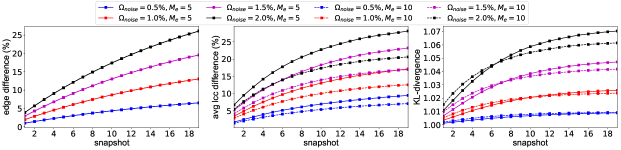
Figure 5: Factors influencing the utility of released graphs.

Effectiveness. Fig. 4 shows the success probability of our attack when different noise ratios are applied on dynamic graphs with different initial sizes and growth speeds. First, we can see that the success probability decreases when more noise is applied. This is natural as more perturbation makes it more difficult to find the correct sybil sugraph, either because the sybil graph has been too perturbed to be found as a candidate or because edge perturbation generates more subgraphs similar to the original sybil subgraph. When $M_{e}=5$ and the noise ratio is set to $0.5\%$, success probability always remains above $0.5$. For this value of $M_{e}$, even with $\Omega_{\it noise}$ at $2.0\%$, the attack still displays success probability above $0.5$ in the first three snapshots. Second, the rate at which success probability decreases slows down as we increase the value of the noise ratio. The largest drop occurs when we increase $\Omega_{\it noise}$ from $0.5$ to $1.0$. This suggests that keeping increasing the level of perturbation may not necessarily guarantee a better privacy protection, but just damage the utility of the released graphs. Third, the sequences of success probability values show a very small dependence on the initial size of the graphs, with other parameters fixed. Last, the success probability decreases when dynamic graphs grow faster. From the figure, we can see that the probability reduces by about $10\%$ when we increase the value of $M_{e}$ from 5 to 10.

Summing up, we observe that the risk of re-identification decreases when more perturbation is applied and when the graphs grow faster, whereas the initial size of the graphs has a relative small impact on this risk.

Utility. We evaluate the utility of released graphs in terms of three measures: the percentage of edge editions, the variation of the average local clustering coefficient, and the KL-divergence of degree distributions. The first measure quantifies the percentage of edge flips with respect to the total number of edges. In fact, it quantifies the amount of noise accumulated so far. For the $t_{i}$-snapshot, the percentage of edge editions is computed as

$$\frac{1}{\!\mid\!E_{G^{+}_{t_{i}}}\mid}\!\mid\!\{(v,v^{\prime})\in E_{G^{+}_{t_{i}}}\mid(\varphi(v),\varphi(v^{\prime}))\not\in{G^{\star}_{t_{i}}}\}\\ \cup\{(v,v^{\prime})\in E_{G^{\star}_{t_{i}}}\mid(\varphi^{-1}(v),\varphi^{-1}(v^{\prime}))\not\in{G^{+}_{t_{i}}}\}\!\mid\!.$$

The local clustering coefficient (LCC) of a vertex measures the proportion of pairs of mutual neighbours of the vertex that are connected by an edge. We calculate the average to the LCCs of all vertices and take the proportion between the differences of the value of the original graph and that of the anonymised graph as, that is

$$\frac{\!\mid\!{\it avgLcc}({G^{+}_{t_{i}}})-{\it avgLcc}({G^{\star}_{t_{i}}})\!\mid\!}{{\it avgLcc}({G^{+}_{t_{i}}})}.$$

where ${\it avgLcc}(G)$ is the average local clustering coefficient of graph $G$. Our last measure uses the KL-divergence [11] as an indicator of the difference between the degree distribution of the original graph and that of the perturbed graph.

As all the three measures present almost identical patterns for different values of $n_{v}$, we only show the results for $n_{v}=8000$. We have two major observations. First, as expected, the values of all three measures increase as the noise accumulates over time, indicating that the utility of released graphs deteriorates. Even with $\Omega_{\it noise}$ set to just $1.0\%$, at the tenth snapshot we can have up to $10\%$ of edges flipped and changes in edge density around $15\%$. At this point, we can say that the utility of released graphs has already been greatly damaged. Second, when dynamic graphs grow faster, the impact of noise becomes smaller, as more legitimate edges offset the impact of noisy edges.

Together with the finding that larger growth speed results in smaller success probability, we can conclude that the social networks that grow fast among releases display a better balance between re-identification risk and the utility of the released graphs.

5.2.3 Results on a real-life dynamic social graph

We make use of a publicly available graph collected from Petster, a website for pet owners to communicate [12], to validate to what extent the results reported in the previous subsection remain valid in a more realistic domain. The Petster dataset is an undirected graph whose vertices represent the pet owners. The vertices are labelled by their joining date, which span from January 2004 to December 2012. The graph is incremental, which means no vertices are removed. It contains 1898 vertices and $16,750$ edges. We take a snapshot every six months.

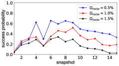
(a) Re-identification risk on Petster.

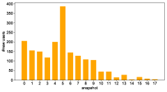
(b) Numbers of new vertices added before release.

Figure 6: Evaluation on Petster.

We present in Fig. 6(a) the success probability of our D-AA attack on the Petster dataset when the noise ratio is set to $0.5\%$, $1.0\%$ and $1.5\%$, respectively. Compared to the success probabilities discussed above on simulated graphs, the curves have different shapes and more fluctuations. This is because, instead of a fixed growth speed (determined by $r_{\Delta}$ and $M_{e}$ in our simulator), the real-life graph grows at different speeds in different periods, as shown in Fig. 6(b). We can see that the number of new vertices varies before each release. After the first few years of steady growth, Petster gradually lost its popularity, especially with few new vertices added in the last three years. By cross-checking the two figures, we can see that the success probability changes with the amount of growth before the corresponding release. It first increases steadily due to the steady growth of the graph until the fifth snapshot, which suddenly has the largest number of new vertices. Then when the growth slows down, the success probability also recovers; and when the growth stops (e.g., from the 12 snapshot), it starts increasing again, even though the noise continues to accumulate. These observations validate our findings on synthetic graphs, that is, the speed of growth is the dominating factor that affects the re-identification risk.

6 Conclusions

In this paper, we have presented the first dynamic active re-identification attack on periodically released social graphs. Unlike preceding attacks, the new attack exploits the inherent dynamic nature of social graphs by leveraging tempo-structural patterns for re-identification. Compared to existing (static) active attacks, our new dynamic attack significantly improves success probability, by more than two times, and efficiency, by almost 10 times. Through comprehensive experimental evaluation on synthetic data, we analysed the factors influencing the success probability of our attack, namely the growth rate of the graph and the amount of noise injected. These findings can subsequently be used to develop graph anonymisation methods that better balance privacy protection and the utility of the released graphs. For instance, for a given noise level, the decision to publish a new snapshot should be determined by taking into account the number of changes that have occurred from the last release. Similarly, if the time for the next release is given, the amount of noise should be customised according to the number of changes that have occurred. Additionally, we evaluated our attack on Petster, a real-life dataset. This evaluation showed that some of the findings obtained on synthetic data remain valid in practical scenarios.

Acknowledgements: The work reported in this paper received funding from Luxembourg’s Fonds National de la Recherche (FNR), via grant C17/IS/11685812 (PrivDA).

References

- [1] Réka Albert and Albert-László Barabási. Statistical mechanics of complex networks. Review of Modern Physics, 74:47–97, 2002.
- [2] Lars Backstrom, Cynthia Dwork, and Jon M. Kleinberg. Wherefore art thou r3579x?: anonymized social networks, hidden patterns, and structural steganography. Communications of the ACM, 54(12):133–141, 2011.
- [3] Jordi Casas-Roma, Jordi Herrera-Joancomartí, and Vicenç Torra. An algorithm for k-degree anonymity on large networks. In Procs. of the 2013 IEEE/ACM Int’l Conf. on Advances in Social Networks Analysis and Mining, pages 671–675, 2013.
- [4] Jordi Casas-Roma, Jordi Herrera-Joancomartí, and Vicenç Torra. k-degree anonymity and edge selection: improving data utility in large networks. Knowledge and Information Systems, 50(2):447–474, 2017.
- [5] Sean Chester, Bruce M Kapron, Ganesh Ramesh, Gautam Srivastava, Alex Thomo, and S Venkatesh. Why waldo befriended the dummy? k-anonymization of social networks with pseudo-nodes. Social Network Analysis and Mining, 3(3):381–399, 2013.
- [6] Narimene Dakiche, Fatima Benbouzid-Si Tayeb, Yahya Slimani, and Karima Benatchba. Tracking community evolution in social networks: A survey. Information Processing & Management, 56(3):1084–1102, 2019.
- [7] Xuan Ding, Lan Zhang, Zhiguo Wan, and Ming Gu. De-anonymizing dynamic social networks. In 2011 IEEE Global Telecommunications Conference-GLOBECOM 2011, pages 1–6. IEEE, 2011.
- [8] Shouling Ji, Weiqing Li, Mudhakar Srivatsa, and Raheem Beyah. Structural data de-anonymization: Quantification, practice, and implications. In Proceedings of the 2014 ACM SIGSAC Conference on Computer and Communications Security, pages 1040–1053. ACM, 2014.
- [9] Shouling Ji, Weiqing Li, Mudhakar Srivatsa, Jing Selena He, and Raheem Beyah. Structure based data de-anonymization of social networks and mobility traces. In International Conference on Information Security, pages 237–254. Springer, 2014.
- [10] Nitish Korula and Silvio Lattanzi. An efficient reconciliation algorithm for social networks. Proceedings of the VLDB Endowment, 7(5):377–388, 2014.
- [11] S. Kullback and R.A. Leibler. On information and sufficiency. The Annals of Mathematical Statistics, 22(1):79–86, 1951.
- [12] Jérôme Kunegis. KONECT: the koblenz network collection. In Proc. 22nd International World Wide Web Conference (WWW), pages 1343–1350. ACM Press, 2013.
- [13] Jure Leskovec, Jon M. Kleinberg, and Christos Faloutsos. Graph evolution: Densification and shrinking diameters. ACM Transactions on Knowledge Discovery from Data (TKDD), 1(1):2, 2007.
- [14] Kun Liu and Evimaria Terzi. Towards identity anonymization on graphs. In Proc. 2008 ACM SIGMOD International Conference on Management of Data (SIGMOD), pages 93–106. ACM Press, 2008.
- [15] Linyuan Lü and Tao Zhou. Link prediction in complex networks: A survey. Physica A: statistical mechanics and its applications, 390(6):1150–1170, 2011.
- [16] Xuesong Lu, Yi Song, and Stéphane Bressan. Fast identity anonymization on graphs. In Procs. of the Int’l Conf. on Database and Expert Systems Applications, pages 281–295, 2012.
- [17] Tinghuai Ma, Yuliang Zhang, Jie Cao, Jian Shen, Meili Tang, Yuan Tian, Abdullah Al-Dhelaan, and Mznah Al-Rodhaan. Kdvem: a k-degree anonymity with vertex and edge modification algorithm. Computing, 97(12):1165–1184, 2015.
- [18] Sjouke Mauw, Yunior Ramírez-Cruz, and Rolando Trujillo-Rasua. Anonymising social graphs in the presence of active attackers. Transactions on Data Privacy, 11(2):169–198, 2018.
- [19] Sjouke Mauw, Yunior Ramírez-Cruz, and Rolando Trujillo-Rasua. Conditional adjacency anonymity in social graphs under active attacks. Knowledge and Information Systems, 61(1):485–511, 2018.
- [20] Sjouke Mauw, Yunior Ramírez-Cruz, and Rolando Trujillo-Rasua. Robust active attacks on social graphs. Data Mining and Knowledge Discovery, 33(5):1357–1392, 2019.
- [21] Arvind Narayanan, Elaine Shi, and Benjamin IP Rubinstein. Link prediction by de-anonymization: How we won the kaggle social network challenge. In The 2011 International Joint Conference on Neural Networks, pages 1825–1834. IEEE, 2011.
- [22] Arvind Narayanan and Vitaly Shmatikov. De-anonymizing social networks. In Proc. 30th IEEE Symposium on Security and Privacy (S&P), pages 173–187. IEEE Computer Society, 2009.
- [23] Shirin Nilizadeh, Apu Kapadia, and Yong-Yeol Ahn. Community-enhanced de-anonymization of online social networks. In Proc. 2014 ACM SIGSAC Conference on Computer and Communications Security (CCS), pages 537–548. ACM Press, 2014.
- [24] Shirin Nilizadeh, Apu Kapadia, and Yong-Yeol Ahn. Community-enhanced de-anonymization of online social networks. In Proceedings of the 2014 acm sigsac conference on computer and communications security, pages 537–548. ACM, 2014.
- [25] Fragkiskos Papadopoulos and Kaj-Kolja Kleineberg. Link persistence and conditional distances in multiplex networks. Physical Review E, 99(1):012322, 2019.
- [26] Pedram Pedarsani, Daniel R Figueiredo, and Matthias Grossglauser. A bayesian method for matching two similar graphs without seeds. In 2013 51st Annual Allerton Conference on Communication, Control, and Computing (Allerton), pages 1598–1607. IEEE, 2013.
- [27] Wei Peng, Feng Li, Xukai Zou, and Jie Wu. Seed and grow: An attack against anonymized social networks. In Procs. of the 9th Annual IEEE Communications Society Conf. on Sensor, Mesh and Ad Hoc Communications and Networks, pages 587–595, 2012.
- [28] Wei Peng, Feng Li, Xukai Zou, and Jie Wu. A two-stage deanonymization attack against anonymized social networks. IEEE Transactions on Computers, 63(2):290–303, 2014.
- [29] François Rousseau, Jordi Casas-Roma, and Michalis Vazirgiannis. Community-preserving anonymization of graphs. Knowledge and Information Systems, 54(2):315–343, 2017.
- [30] Julián Salas and Vicenç Torra. Graphic sequences, distances and k-degree anonymity. Discrete Applied Mathematics, 188:25–31, 2015.
- [31] Chih-Hua Tai, Peng-Jui Tseng, S Yu Philip, and Ming-Syan Chen. Identities anonymization in dynamic social networks. In 2011 IEEE 11th International Conference on Data Mining, pages 1224–1229. IEEE, 2011.
- [32] Rolando Trujillo-Rasua and Ismael González Yero. k-metric antidimension: A privacy measure for social graphs. Information Sciences, 328:403–417, 2016.
- [33] Yazhe Wang, Long Xie, Baihua Zheng, and Ken CK Lee. High utility k-anonymization for social network publishing. Knowledge and Information Systems, 41(3):697–725, 2014.
- [34] Wentao Wu, Yanghua Xiao, Wei Wang, Zhenying He, and Zhihui Wang. K-symmetry model for identity anonymization in social networks. In Procs. of the 13th Int’l Conf. on Extending Database Technology, pages 111–122, 2010.
- [35] Lyudmila Yartseva and Matthias Grossglauser. On the performance of percolation graph matching. In Proceedings of the first ACM conference on Online social networks, pages 119–130. ACM, 2013.
- [36] Haifeng Yu, Phillip B Gibbons, Michael Kaminsky, and Feng Xiao. Sybillimit: A near-optimal social network defense against sybil attacks. In Procs. of the 2008 IEEE Symposium on Security and Privacy, pages 3–17, Oakland, CA, USA, 2008.
- [37] Haifeng Yu, Michael Kaminsky, Phillip B Gibbons, and Abraham Flaxman. Sybilguard: defending against sybil attacks via social networks. In Procs. of the 2006 Conf. on Applications, Technologies, Architectures, and Protocols for Computer Communications, pages 267–278, Pisa, Italy, 2006.
- [38] Bin Zhou and Jian Pei. Preserving privacy in social networks against neighborhood attacks. In Procs. of the 2008 IEEE 24th Int’l Conf. on Data Engineering, pages 506–515, Washington, DC, USA, 2008.
- [39] Lei Zou, Lei Chen, and M. Tamer Özsu. K-automorphism: A general framework for privacy preserving network publication. PVLDB, 2(1):946–957, 2009.