Safe Linear Stochastic Bandits

Abstract

We introduce the safe linear stochastic bandit framework—a generalization of linear stochastic bandits—where, in each stage, the learner is required to select an arm with an expected reward that is no less than a predetermined (safe) threshold with high probability. We assume that the learner initially has knowledge of an arm that is known to be safe, but not necessarily optimal. Leveraging on this assumption, we introduce a learning algorithm that systematically combines known safe arms with exploratory arms to safely expand the set of safe arms over time, while facilitating safe greedy exploitation in subsequent stages. In addition to ensuring the satisfaction of the safety constraint at every stage of play, the proposed algorithm is shown to exhibit an expected regret that is no more than $O(\sqrt{T}\log(T))$ after $T$ stages of play.

1 Introduction

We investigate the role of safety in constraining the design of learning algorithms within the classical framework of linear stochastic bandits (?; ?; ?). Specifically, we introduce a family of safe linear stochastic bandit problems where—in addition to the typical goal of designing learning algorithms that minimize regret—we impose a constraint requiring that an algorithm’s stagewise expected reward remains above a predetermined safety threshold with high probability at every stage of play. In the proposed framework, we assume that a “safe” baseline arm is initially known, and consider a class of safety thresholds that are defined as fixed cutbacks on the expected reward of the known baseline arm. Accordingly, an algorithm that is deemed to be safe cannot induce stagewise rewards that dip below the baseline reward by more than a fixed amount. Critically, the assumption of a known baseline arm—and the limited capacity for exploration implied by the class of safety thresholds considered—can be leveraged on to initially guide the exploration of allowable arms by playing combinations of the baseline arm and exploratory arms in a manner that expands the set of safe arms over time, while simultaneously preserving safety at every stage of play.

There are a variety of real-world applications that might benefit from the design of stagewise-safe online learning algorithms (?; ?; ?). Most prominently, clinical trials have long been used as a motivating application for the multi-armed bandit (?) and linear bandit (?) frameworks. However, as pointed out by (?): “Despite this apparent near-perfect fit between a real-world problem and a mathematical theory, the MABP has yet to be applied to an actual clinical trial.” One could argue that the ability to provide a learning algorithm that is guaranteed to be stagewise safe has the potential to facilitate the utilization of bandit models and algorithms in clinical trials. More concretely, consider the possibility of using the linear bandit framework to model the problem of optimizing a combination of $d$ candidate treatments for a specific health issue. In this context, an “arm” represents a mixture of treatments, the “unknown reward vector” encodes the effectiveness of each treatment, and the “reward” represents a patient’s response to a chosen mixture of treatments. In terms of the safety threshold, it is natural to select the “baseline arm” to be the (possibly suboptimal) combination of treatments possessing the largest reward known to date. As it is clearly unethical to prescribe a treatment that may degrade a patient’s health, the stagewise safety constraint studied in this paper can be interpreted as a requirement that a patient’s response to a chosen treatment must be arbitrarily close to that of the baseline treatment, if not better.

1.1 Contributions

In this paper, we propose a new learning algorithm that is tailored to the safe linear bandit framework. The proposed algorithm, which we call the Safe Exploration and Greedy Exploitation (SEGE) algorithm, is shown to exhibit near-optimal expected regret, while guaranteeing the satisfaction of the proposed safety constraint at every stage of play. Initially, the SEGE algorithm performs safe exploration by combining the baseline arm with a random exploratory arm that is constrained by an “exploration budget” implied by the stagewise safety constraint. Over time, the proposed algorithm systematically expands the family of safe arms in this manner to include new safe arms with expected rewards that exceed the baseline reward level. Exploitation under the SEGE algorithm is based on the certainty equivalence principle. That is, the algorithm constructs an “estimate” of the unknown reward parameter, and selects an arm that is optimal for the given parameter estimate. The SEGE algorithm only plays the certainty equivalent (i.e., greedy) arm when it is safe—a condition that is determined according to a lower confidence bound on its expected reward. Moreover, the proposed algorithm balances the trade-off between exploration and exploitation by controlling the rate at which information is accumulated over time, as measured by the growth rate of the minimum eigenvalue of the so-called information matrix. More specifically, the SEGE algorithm guarantees that the minimum eigenvalue of the information matrix grows at a rate ensuring that the expected regret of the algorithm is no greater than $O(\sqrt{T}\log(T))$ after $T$ stages of play. This regret rate that is near optimal in light of $\Omega(\sqrt{T})$ lower bounds previously established in the linear stochastic bandit literature (?; ?).

1.2 Related Literature

There is an extensive literature on linear stochastic bandits. For this setting, several algorithms based on the principle of Optimism in the Face of Uncertainty (OFU) (?; ?; ?) or Thompson Sampling (?) have been proposed. Although such algorithms are known to be near-optimal under various measures of regret, they may fail in the safe linear bandit framework, as their (unconstrained) approach to exploration may result in a violation of the stagewise safety constraints considered in this paper.

In the context of multi-armed bandits, there is a related stream of literature that focuses on the design of “risk-sensitive” learning algorithms by encoding risk in the performance objectives according to which regret is measured (?; ?). Typical risk measures that have been studied in the multi-armed bandit literature include Mean-Variance (?; ?), Value-at-Risk (?), and Conditional Value-at-Risk (?). Although such risk-sensitive algorithms are inclined to exhibit reduced volatility in the cumulative reward that is received over time, they are not constrained in a manner that explicitly limits the stagewise risk of the reward processes that they induce.

Closer to the setting studied in this paper is the conservative bandit framework (?; ?), which incorporates explicit safety constraints on the reward process induced by the learning algorithm. However, in contrast to the stagewise safety constraints considered in this paper, conservative bandits encode their safety requirements in the form of constraints on the cumulative rewards received by the algorithm. Along a similar line of research, (?) investigate the design of learning algorithms for risk-constrained contextual bandits that balance a tradeoff between cumulative constraint violation and regret. Given the cumulative nature of the safety constraints considered by the aforementioned algorithms, they cannot be directly applied to the stagewise safe linear bandit problem considered in this paper. In Section 6.3, we provide a simulation-based comparison between the SEGE algorithm and the Conservative Linear Upper Confidence Bound (CLUCB) algorithm (?) to more clearly illustrate the potential weaknesses and strengths of each approach.

We close this section by mentioing another closely related body of work in the online learning literature that investigates the design of stagewise-safe algorithms for a more general class of smooth reward functions (?; ?; ?). Although the proposed algorithms are shown to respect stagewise safety constraints that are similar in spirit to the class of safety constraints considered in this paper, they lack formal upper bounds on their cumulative regret.

1.3 Organization

The remainder of the paper is organized as follows. We introduce pertinent notation in Section 2. In Section 3, we define the safe linear stochastic bandit problem. In Section 4, we introduce the Safe Exploration and Greedy Exploitation (SEGE) algorithm. We present our main theoretical findings in Section 5, and close the paper with a simulation study of the SEGE algorithm in Section 6. All mathematical proofs are presented in the Appendix to the paper.

2 Notation

We denote the standard Euclidean norm of a vector $x\in\mathbb{R}^{d}$ by $\lVert x\rVert$ and define its weighted Euclidean norm as $\lVert x\rVert_{S}=\sqrt{x^{\top}Sx}$ where $S\in\mathbb{R}^{d\times d}$ is a given symmetric positive semidefinite matrix. We denote the inner product of two vectors $x,y\in\mathbb{R}^{d}$ by $\langle x,y\rangle=x^{\top}y$. For a square matrix $A\in\mathbb{R}^{d\times d}$, we denote its minimum and maximum eigenvalues by $\lambda_{\min}(A)$ and $\lambda_{\max}(A)$, respectively.

3 Problem Formulation

In this section, we introduce the safe linear stochastic bandit model considered in this paper. Before doing so, we review the standard model for linear stochastic bandits on which our formulation is based.

3.1 Linear Bandit Model

Linear stochastic bandits belong to a class of sequential decision-making problems in which a learner (i.e., decision-maker) seeks to maximize an unknown linear function using noisy observations of its function values that it collects over multiple stages. More precisely, at each stage $t=1,2,\dots$, the learner is required to select an arm (i.e., action) $X_{t}$ from a compact set $\mathcal{X}\subset\mathbb{R}^{d}$ of allowable arms, which is assumed to be an ellipsoid of the form

$$\mathcal{X}=\left\{x\in\mathbb{R}^{d}\ |\ (x-\bar{x})^{\top}H^{-1}(x-\bar{x})\leq 1\right\},$$ (1)

where $\bar{x}\in\mathbb{R}^{d}$ and $H\in\mathbb{R}^{d\times d}$ is a symmetric and positive definite matrix. In response to the particular arm played at each stage $t$, the learner observes a reward $Y_{t}$ that is induced by the stochastic linear relationship:

$$Y_{t}=\langle X_{t},\theta^{*}\rangle+\eta_{t}.$$ (2)

Here, the noise process $\{\eta_{t}\}_{t=1}^{\infty}$ is assumed be a sequence of independent and zero-mean random variables, and, critically, the reward parameter $\theta^{*}\in\mathbb{R}^{d}$ is assumed to be fixed and unknown. This a priori uncertainty in the reward parameter gives rise to the need to balance the exploration-exploitation trade-off in adaptively guiding the sequence of arms played in order to maximize the expected reward accumulated over time.

Admissible Policies and Regret.

We restrict the learner’s decisions to those which are non-anticipating in nature. That is to say, at each stage $t$, the learner is required to select an arm based only on the history of past observations $H_{t}=(X_{1},Y_{1},\dots,X_{t-1},Y_{t-1})$, and on an external source of randomness encoded by a random variable $U_{t}$. The random process $\{U_{t}\}_{t=1}^{\infty}$ is assumed to be independent across time, and independent of the random noise process $\{\eta_{t}\}_{t=1}^{\infty}$. Formally, an admissible policy is a sequence of functions $\pi=\{\pi_{t}\}_{t=1}^{\infty}$, where each function $\pi_{t}$ maps the information available to the learner at each stage $t$ to a feasible arm $X_{t}\in\mathcal{X}$ according to $X_{t}=\pi_{t}(H_{t},U_{t})$.

The performance of an admissible policy after $T$ stages of play is measured according to its expected regret, which equals the difference between the expected reward accumulated by the optimal arm and the expected reward accumulated by the given policy after $T$ stages of play. Formally, the expected regret of an admissible policy is defined as

$$R_{T}=\sum_{t=1}^{T}\langle X^{*},\theta^{*}\rangle-\mathbb{E}\left[\sum_{t=1}^{T}\langle X_{t},\theta^{*}\rangle\right],$$ (3)

where expectation is taken with respect to the distribution induced by the underling policy, and $X^{*}\in\mathcal{X}$ denotes the optimal arm that maximizes the expected reward at each stage of play given knowledge of the reward parameter $\theta^{*}$, i.e.,

$$X^{*}=\mbox{argmax}_{x\in\mathcal{X}}\langle x,\theta^{*}\rangle.$$ (4)

At a minimum, we seek policies exhibiting an expected regret that is sublinear in the number of stages played $T$. Such policies are said to have no-regret in the sense that $\lim_{T\rightarrow\infty}\ R_{T}/T=0$. To facilitate the design and theoretical analysis of such policies, we adopt a number of technical assumptions, which are standard in the literature on linear stochastic bandits, and are assumed to hold throughout the paper.

Assumption 1

The unknown reward parameter is bounded according to $\|\theta^{*}\|\leq S$, where $S>0$ is a known constant.

Assumption 1 will prove essential to the design of policies that safely explore the parameter space in a manner ensuring that the expected reward stays above a predetermined (safe) threshold with high probability at each stage of play. We refer the reader to Definition 1 for a formal definition of the particular safety notion considered in this paper.

Assumption 2

Each element of $\{\eta_{t}\}_{t=1}^{\infty}$ is assumed to be $\sigma_{\eta}$-sub-Gaussian, where $\sigma_{\eta}\geq 0$ is a fixed constant. That is,

$$\mathbb{E}\left[\exp(\gamma\eta_{t})\right]\leq\exp\left(\gamma^{2}\sigma_{\eta}^{2}/2\right)$$

for all $\gamma\in\mathbb{R}$ and $t\geq 1$.

Assumptions 1 and 2, together with the class of admissible policies considered in this paper, enable the utilization of existing results that provide an explicit characterization of confidence ellipsoids for the unknown reward parameter based on a $\ell_{2}$-regularized least-squares estimator (?). Such confidence regions play a central role in the design of no-regret algorithms for the linear stochastic bandits (?; ?; ?).

3.2 Safe Linear Bandit Model

In what follows, we introduce the framework of safe linear stochastic bandits studied in this paper. Loosely speaking, an admissible policy is said to be safe if the expected reward $\mathbb{E}\left[Y_{t}\mid X_{t}\right]=\langle X_{t},\theta^{*}\rangle$ that it induces at each stage $t$ is guaranteed to stay above a given reward threshold with high probability. More formally, we have the following definition.

Definition 1 (Stagewise Safety Constraint)

Let $b\in\mathbb{R}$ and $\delta\in[0,1]$. An admissible policy $\pi$—or equivalently the arm $X_{t}$ that it induces—is defined to be $(\delta,b)$-safe at stage $t$ if

$$\mathbb{P}\left(\langle X_{t},\theta^{*}\rangle\geq b\right)\geq 1-\delta,$$ (5)

where the probability is calculated according to the distribution induced by the policy $\pi$.

The stagewise safety constraint requires that the expected reward at stage $t$ exceed the safety threshold $b\in\mathbb{R}$ with probability no less than $1-\delta$, where $\delta\in[0,1]$ encodes the maximum allowable risk that the learner is willing to tolerate.

Clearly, without making additional assumptions, it is not possible to design policies that are guaranteed to be safe according to (5) given arbitrary safety specifications. We circumvent this obvious limitation by giving the learner access to a baseline arm with a known lower bound on its expected reward. We formalize this assumption as follows.

Assumption 3 (Baseline Arm)

We assume that the learner knows a deterministic baseline arm $X_{0}\in\mathcal{X}$ satisfying

$$\langle X_{0},\theta^{*}\rangle\geq b_{0},$$

where $b_{0}\in\mathbb{R}$ is a known lower bound on its expected reward.

We note that it is straightforward to construct a baseline arm satisfying Assumption 3 by leveraging on the assumed boundedness of the unknown reward parameter as specified by Assumption 1. In particular, any arm $X_{0}\in\mathcal{X}$ and its corresponding “worst-case” reward given by $b_{0}=\min_{\|\theta\|\leq S}\ \langle X_{0},\theta\rangle=-S\|X_{0}\|$ are guaranteed to satisfy Assumption 3.

With Assumption 3 in hand, the learner can leverage on the baseline arm to initially guide its exploration of allowable arms by playing combinations of the baseline arm and carefully designed exploratory arms in a manner that safely expands the set of safe arms over time. Plainly, the ability to safely explore in the vicinity of the baseline arm is only possible under stagewise safety constraints defined in terms of safety thresholds satisfying $b<b_{0}$. Under such stagewise safety constraints, the difference in rewards levels $b_{0}-b$ can be interpreted as a stagewise “exploration budget” of sorts, as it reflects the maximum relative loss in expected reward that the learner is willing to tolerate when playing arms that deviate from the baseline arm. Naturally, the larger the exploration budget, the more aggressively can the learner explore. With the aim of designing safe learning algorithms that leverage on this simple idea, we will restrict our attention to stagewise safety constraints that are specified in terms of safety thresholds satisfying $b<b_{0}$.

Before proceeding, we briefly summarize the framework of safe linear stochastic bandits considered in this paper. Given a baseline arm satisfying Assumption 3, the learner is initially required to fix a safety threshold that satisfies $b<b_{0}$. At each subsequent stage $t=1,2,\dots$, the learner must select a risk level $\delta_{t}\in[0,1]$ and a corresponding arm $X_{t}\in\mathcal{X}$ that is $(\delta_{t},b)$-safe. The learner aims to design an admissible policy that minimizes its expected regret, while simultaneously ensuring that all arms played satisfy the stagewise safety constraints. In the following section, we propose a policy that is guaranteed to both exhibit no-regret and satisfy the safety constraint at every stage of play.

Relationship to Conservative Bandits.

We briefly discuss the relationship between the safety constraints considered in this paper and the conservative bandit framework orginally studied by (?) in the context of multi-armed bandits, and subsequently extended to the setting of linear bandits by (?). In contrast to the stagewise safety constraints considered in this paper, conservative bandits encode their safety requirements in the form of constraints on the cumulative expected rewards received by a policy. Specifically, given a baseline arm satisfying Assumption 3, an admissible policy is said to respect the safety constraint defined in (?) if

$$\mathbb{P}\left(\sum_{k=1}^{t}\langle X_{k},\theta^{*}\rangle\geq(1-\alpha)\sum_{k=1}^{t}b_{0},\ \forall\ t\geq 1\right)\geq 1-\delta,$$ (6)

where $\delta\in[0,1]$ and $\alpha\in(0,1)$. Here, the parameter $\alpha$ encodes the maximum fraction of the cumulative baseline rewards that the learner is willing to forgo over time. In this context, smaller values of $\alpha$ imply greater levels of conservatism (safety). It is straightforward to show that conservative performance constraints of the form (6) are a special case of the class of stagewise safety constraints considered in Definition 1. In particular, if we set the safety threshold according to $b=(1-\alpha)b_{0}$, and let $\{\delta_{t}\}_{t=1}^{\infty}$ be any summable sequence of risk levels satisfying $\sum_{t=1}^{\infty}\delta_{t}\leq\delta$, then any admissible policy that is $(\delta_{t},b)$-safe for each stage $t\geq 1$ also satisfies the conservative performance constraint (6).

4 A Safe Linear Bandit Algorithm

In this section, we propose a new algorithm, which we call the Safe Exploration and Greedy Exploitation (SEGE) algorithm, that is guaranteed to be safe in every stage of play, while exhibiting a near-optimal expected regret. Before proceeding with a detailed description of the proposed algorithm, we briefly summarize the basic elements underpinning its design. Initially, the SEGE algorithm performs safe exploration by playing convex combinations of the baseline arm and random exploratory arms in a manner that satisfies Definition 1. Through this process of exploration, the SEGE algorithm is able to expand the family of safe arms to incorporate new arms that are guaranteed to outperform the baseline arm with high probability. Among all safe arms available to the algorithm at any given stage of play, the arm with the largest lower confidence bound on its expected reward is used as the basis for safe exploration. The SEGE algorithm performs exploitation by playing the certainty equivalent (greedy) arm based on a $\ell_{2}$-regularized least-squares estimate of the unknown reward parameter. The SEGE algorithm only plays the greedy arm when it is safe, i.e., when a lower confidence bound on its expected reward exceeds the given safety threshold. Critically, the proposed algorithm balances the trade-off between exploration and exploitation by explicitly controlling the growth rate of the so-called information matrix (cf. Eq. (8)) in a manner that ensures that the expected regret of the SEGE algorithm is no greater than $O(\sqrt{T}\log(T))$ after $T$ stages of play. The pseudocode for the SEGE algorithm is presented in Algorithm 1.

In the following section, we introduce a regularized least-squares estimator that will serve as the foundation for the proposed learning algorithm.

4.1 Regularized Least Squares Estimator

The $\ell_{2}$-regularized least-squares estimate of the unknown reward parameter $\theta^{*}$ based on the information available to the algorithm up until and including stage $t$ is defined as

$$\widehat{\theta}_{t}=\underset{\theta\in\mathbb{R}^{d}}{\mbox{argmin}}\ \left\{\sum_{k=1}^{t}(Y_{k}-\langle X_{k},\theta\rangle)^{2}+\lambda\lVert\theta\rVert^{2}\right\}.$$

Here, $\lambda>0$ denotes a user-specified regularization parameter. It is straightforward to show that

$$\widehat{\theta}_{t}=V_{t}^{-1}\sum_{k=1}^{t}X_{k}Y_{k},$$ (7)

where

$$V_{t}=\lambda I+\sum_{k=1}^{t}X_{k}X_{k}^{\top}.$$ (8)

Throughout the paper, we will frequently refer to the matrix $V_{t}$ as the information matrix at each stage $t$.

The following result taken from (?, Theorem 2) provides an ellipsoidal characterization of a confidence region for the unknown reward parameter based on the regularized least-squares estimator (7). It is straightforward to verify that the conditions of (?, Theorem 2) are satisfied under the standing assumptions of this paper.

Theorem 1

For any admissible policy and $\delta\in(0,1)$, it holds that

$$\mathbb{P}\left(\theta^{*}\in\mathcal{C}_{t}(\delta),\ \forall t\geq 1\right)\geq 1-\delta,$$

where the confidence set $\mathcal{C}_{t}(\delta)$ is defined as

$$\mathcal{C}_{t}(\delta)=\left\{\theta\in\mathbb{R}^{d}\ :\ \lVert\widehat{\theta}_{t}-\theta\rVert_{V_{t}}\leq r_{t}(\delta)\right\}.$$ (9)

Here, $r_{t}(\delta)$ is defined as

$$r_{t}(\delta)=\sigma_{\eta}\sqrt{d\log\left(\frac{1+tL^{2}/\lambda}{\delta}\right)}+\sqrt{\lambda}S,$$ (10)

where $L=\max_{x\in\mathcal{X}}{\lVert x\rVert}$.

In the following section, we propose a method for safe exploration using the characterization of the confidence ellipsoids introduced in Theorem 1.

4.2 Safe Exploration

We now describe the approach to “safe exploration” that is employed by the proposed algorithm. At each stage $t\geq 1$, given a risk level $\delta_{t}$, the SEGE algorithm constructs a safe exploration arm ($X^{\mathsf{SE}}_{t}$) as a convex combination of a $(\delta_{t},b_{0})$-safe arm ($X^{\mathsf{S}}_{t}$) and a random exploratory arm ($U_{t}$), i.e.,

$$X^{\mathsf{SE}}_{t}=(1-\rho)X^{\mathsf{S}}_{t}+\rho U_{t}.$$ (11)

Qualitatively, the user-specified parameter $\rho\in(0,1)$ controls the balance between safety and exploration. Figure 1 provides a graphical illustration of the set of all safe exploration arms induced by a given safe arm $X^{\mathsf{S}}_{t}$ according to (11).

The random exploratory arm process $\{U_{t}\}_{t=1}^{\infty}$ is generated according to

$$U_{t}=\bar{x}+H^{1/2}\zeta_{t},$$ (12)

where the random process $\{\zeta_{t}\}_{t=1}^{\infty}$ is assumed to be a sequence of independent, zero-mean, and symmetric random vectors. For each element of the sequence, we require that $\lVert\zeta_{t}\rVert=1$ almost surely and $\sigma_{\zeta}^{2}=\lambda_{\min}(\mbox{Cov}\left(\zeta_{t}\right))>0$. Additionally, we define $\sigma^{2}=\lambda_{\min}(\mbox{Cov}\left(U_{t}\right))$. The parameters $\sigma$ and $\rho$ both determine how aggressively the algorithm can explore the set of allowable arms. However, exploration that is too aggressive may result in a violation of the stagewise safety constraint. In the following Lemma, we establish an upper bound on $\rho$ such that for all choices of $\rho\in(0,\bar{\rho})$, the arm $X^{\mathsf{SE}}_{t}$ is guaranteed to be safe for any $\sigma\geq 0$.

Lemma 1

Let $\rho\in(0,\bar{\rho})$ where $\bar{\rho}>0$ is defined as

$$\bar{\rho}=\min\ \left\{1,\frac{b_{0}-b}{2S\sqrt{\lambda_{\max}(H)}}\right\}.$$ (13)

Then, for every stage $t\geq 1$, the safe exploration arm $X^{\mathsf{SE}}_{t}$ defined in Equation (11) is $(\delta,b)$-safe for any $\delta\in[0,1]$.

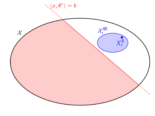
Figure 1: The figure illustrates the effect of the safety constraint on the learner’s decision making ability. The shaded blue ellipse $\mathcal{X}^{\mathsf{SE}}_{t}$ depicts the set of all safe exploration arms constructed using the safe arm $X^{\mathsf{S}}_{t}$ under the SEGE algorithm, i.e., $\mathcal{X}^{\mathsf{SE}}_{t}=\{(1-\rho)X^{\mathsf{S}}_{t}+\rho x\mid\rho\in(0,\bar{\rho}),x\in\partial\mathcal{X}\}$. The red shaded area depicts the set of unsafe arms. The black ellipse (and its interior) depicts the set of feasible arms.

As the SEGE algorithm expands its set of safe arms over time, it attempts to increase the stagewise efficiency with which it safely explores by exploring in the vicinity of the safe arm with the largest lower confidence bound on its expected reward. More specifically, at each stage $t$, the SEGE algorithm constructs a confidence set $\mathcal{C}_{t-1}(\delta_{t})$ according to Equation (9). With this confidence set in hand, the proposed algorithm calculates a lower confidence bound (LCB) on the expected reward $\mbox{LCB}_{t}(x)$ of each arm $x\in\mathcal{X}$ according to

$$\mbox{LCB}_{t}(x)=\min_{\theta\in\mathcal{C}_{t-1}(\delta_{t})}\ \langle x,\theta\rangle.$$

It is straightforward to show that the lower confidence bound defined above can be simplified to:

$$\mbox{LCB}_{t}(x)=\langle x,\widehat{\theta}_{t-1}\rangle-r_{t}(\delta_{t})\lVert x\rVert_{V_{t-1}^{-1}}.$$

We define the LCB arm ($X^{\mathsf{LCB}}_{t}$) to be the arm with the largest lower confidence bound on its expected reward among all allowable arms. It is given by:

$$X^{\mathsf{LCB}}_{t}=\mbox{argmax}_{x\in\mathcal{X}}\ \mbox{LCB}_{t}(x).$$ (14)

Clearly, the LCB arm is guaranteed to be $(\delta_{t},b_{0})$-safe if $\mbox{LCB}_{t}(X^{\mathsf{LCB}}_{t})\geq b_{0}$. In this case, the SEGE algorithm relies on the LCB arm for safe exploration, as its expected reward is potentially superior to the baseline arm’s expected reward. Putting everything together, the SEGE algorithm sets the safe arm ($X^{\mathsf{S}}_{t}$) at each stage $t$ according to:

$$X^{\mathsf{S}}_{t}=\begin{cases}X^{\mathsf{LCB}}_{t},&\text{if}\ \ \mbox{LCB}_{t}(X^{\mathsf{LCB}}_{t})\geq b_{0},\\ X_{0},&\text{otherwise}.\end{cases}$$ (15)

Before closing this section, it is important to note that the LCB arm (14) can be calculated in polynomial time by solving a second-order cone program. This is in stark contrast to the non-convex optimization problem that needs to be solved when computing the UCB arm (i.e., the arm with the largest upper confidence bound on the expected reward)—a problem that has been shown to be NP-hard in general (?).

4.3 Safe Greedy Exploitation

We now describe the method for exploitation employed by the SEGE algorithm. Exploitation under the SEGE algorithm relies on the certainty equivalence principle. That is, the algorithm first estimates the unknown reward parameter according to Equation (7). Then, the algorithm chooses an arm that is optimal for the given parameter estimate. Given the ellipsoidal structure of the set of allowable arms, the optimal arm $X^{*}$ can be calculated as

$$X^{*}=\bar{x}+\frac{H\theta^{*}}{\lVert\theta^{*}\rVert_{H}}.$$ (16)

Similarly, the certainty equivalent (greedy) arm can be calculated as

$$X^{\mathsf{CE}}_{t}=\bar{x}+\dfrac{H\widehat{\theta}_{t-1}}{\lVert\widehat{\theta}_{t-1}\rVert_{H}},$$ (17)

where $\widehat{\theta}_{t-1}$ is the regularized least-squares estimate of the unknown reward parameter, as defined in Equation (7).

It is important to note that the SEGE algorithm only plays the greedy arm (17) when the lower confidence bound on its expected reward is greater than or equal to the safety threshold $b$. This ensures that the greedy arm is only played when it is safe.

Algorithm 1 SEGE Algorithm

1:  Input: $X_{0}$, $b_{0}$, $\mathcal{X}$, $S>0$, $c>0$, $\lambda>0$, $b<b_{0}$, $\rho\in(0,\bar{\rho})$, $\delta_{t}\in[0,1]\ \forall t\geq 1$

2:  for $t=1,2,3,\ldots$ do {Parameter Estimation}

3:    Set $\widehat{\theta}_{t-1}$ according to Eq. (7)

4:    Set $\mathcal{C}_{t-1}(\delta_{t})$ according to Eq. (9) {Safe Greedy Exploitation}

5:    if $\mbox{LCB}_{t}(X^{\mathsf{CE}}_{t})\geq b$ and $\lambda_{\min}(V_{t})\geq c\sqrt{t}$

6:      Set $X_{t}=X^{\mathsf{CE}}_{t}$ according to Eq. (17) {Safe Exploration}

7:    else

8:      Set $X_{t}=X^{\mathsf{SE}}_{t}$ according to Eq. (11)

9:    end if

10:    Observe $Y_{t}=\langle X_{t},\theta^{*}\rangle+\eta_{t}$

11:  end for

5 Theoretical Results

We now present our main theoretical results showing that the SEGE algorithm exhibits near optimal regret for a large class of risk levels (cf. Theorem 3), in addition to being safe at every stage of play (cf. Theorem 2). As an immediate corollary to Theorem 3, we establish sufficient conditions under which the SEGE algorithm is also guaranteed to satisfy the conservative bandit constraint (6), while preserving the upper bound on regret in Theorem 3 (cf. Corollary 1).

Theorem 2 (Stagewise Safety Guarantee)

The SEGE algorithm is $(\delta_{t},b)$-safe at each stage, i.e.,

$$\mathbb{P}\left(\langle X_{t},\theta^{*}\rangle\geq b\right)\geq 1-\delta_{t}$$

for all $t\geq 1$.

The ability to enforce safety in the sequence of arms played is not surprising given the assumption of a known baseline arm that is guaranteed to be safe at the outset. However, given the potential suboptimality of the baseline arm, a naïve policy that plays the baseline arm at every stage will likely incur an expected regret that grows linearly with the number of stages played $T$. In constrast, we show, in Theorem 3, that the SEGE algorithm exhibits an expected regret that is no greater than $O(\sqrt{T}\log(T))$ after $T$ stages—a regret rate that is near optimal given existing $\Omega(\sqrt{T})$ lower bounds on regret (?; ?).

Theorem 3 (Upper Bound on Expected Regret)

Fix $\overline{\delta}\in(0,1]$ and $K\geq 0$. Let $\{\delta_{t}\}_{t=1}^{\infty}$ be any sequence of risk levels satisfying

$$\delta_{t}\geq\overline{\delta}e^{-K\sqrt{t}}$$ (18)

for all $t\geq 1$. Then, there exists finite positive constant $C$ such that the expected regret of the SEGE algorithm is upper bounded as

$$R_{T}\leq C\sqrt{T}\log(T)$$ (19)

for all $T\geq 1$.

In what follows, we provide a high-level sketch of the proof of Theorem 3. The complete proof is presented in Appendix A.3. We bound the expected regret incurred during the safe exploration and the greedy exploitation stages separately. First, we show that the stagewise expected regret incurred when playing the greedy arm is proportional to the mean squared parameter estimation error. We then employ Theorem 1 to show that, conditioned on the event $\{\lambda_{\min}(V_{t})\geq c\sqrt{t}\}$, the mean squared parameter estimation error at each stage $t$ is no greater than $O(\log(t)/\sqrt{t})$. It follows that the cumulative expected regret incurred during the exploitation stages is no more than $O(\sqrt{T}\log(T))$ after $T$ stages of play. Now, in order to upper bound the expected regret accumulated during the safe exploration stages, it suffices to upper bound the expected number of safe exploration stages, since the stagewise regret can be upper bounded by a finite constant under any admissible policy. We show that the expected number of safe exploration stages is no more than $O(\sqrt{T})$ after $T$ stages of play for any sequence of risk levels that does not decay faster than the rate specified in (18).

We close this section with a result establishing sufficient conditions under which the SEGE algorithm is guaranteed to satisfy the conservative performance constraint (6), in addition to being stagewise safe, while satisfying an upper bound on its expected regret that matches that of the CLUCB algorithm (?)[Theorem 5]. Corollary 1 is stated without proof, as it is an immediate consequence of Theorems 2 and 3.

Corollary 1 (Conservative Performance Guarantee)

Let $\delta\in(0,1)$. Assume, in addition to the standing assumptions of Theorem 3, that $\{\delta_{t}\}_{t=1}^{\infty}$ is a summable sequence satisfying $\sum_{t=1}^{\infty}\delta_{t}\leq\delta$. Then, the SEGE algorithm satisfies the conservative performance constraint (6), and exhibits an expected regret that is upper bounded by $O(\sqrt{T}\log(T))$ for all $T\geq 1$.

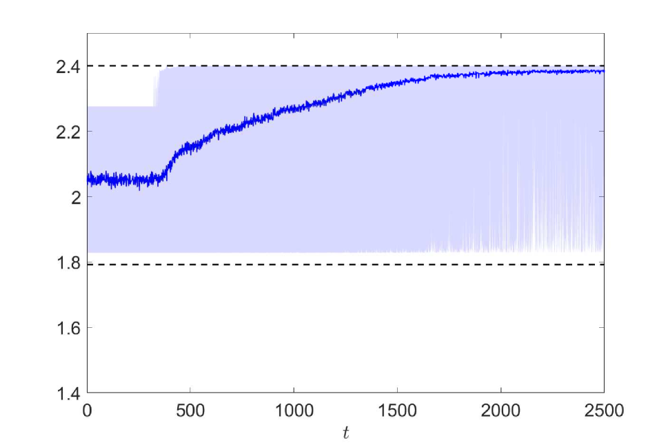
(a) Stagewise expected reward under the SEGE algorithm.

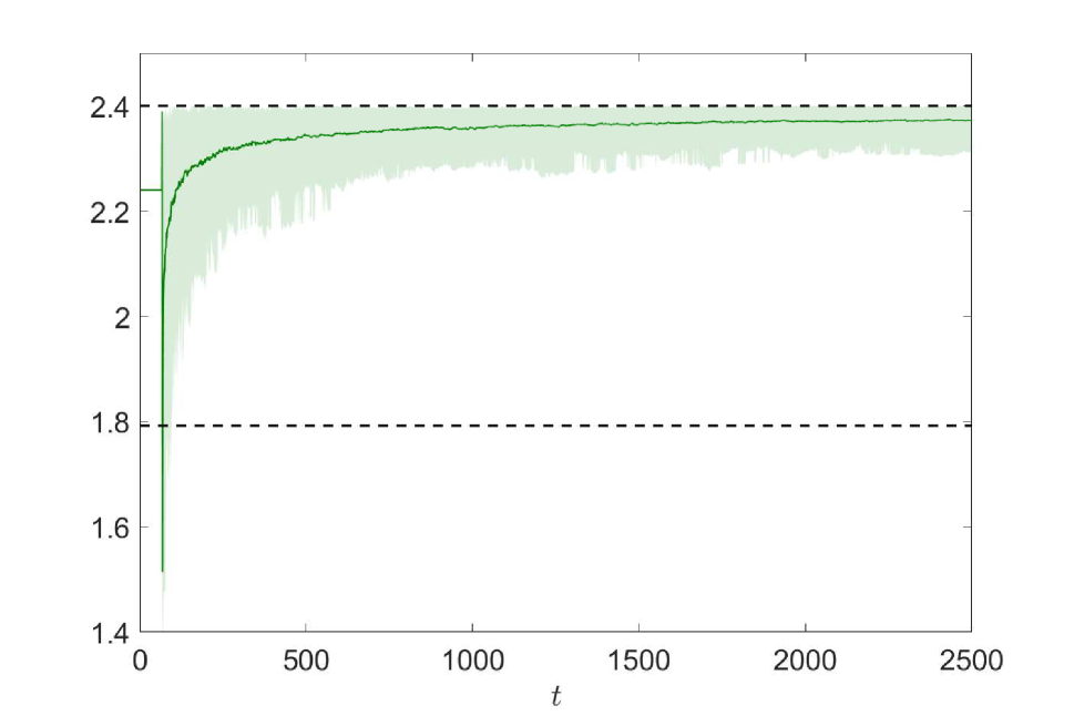
(b) Stagewise expected reward under the CLUCB algorithm.

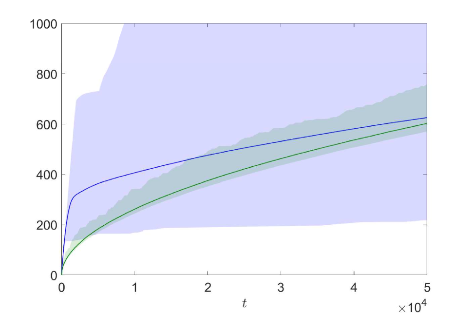
(c) Cumulative regret of the SEGE algorithm (blue) and the CLUCB algorithm (green).

Figure 2: These figures illustrate the empirical performance of the SEGE and CLUCB algorithms. The solid lines depict empirical means and the shaded regions depict empirical ranges computed from $250$ independent simulations.

6 Simulation Results

In this section, we conduct a simple numerical study to illustrate the qualitative features of the SEGE algorithm and compare it with the CLUCB algorithm introduced by (?).

6.1 Simulation Setup

Model Parameters.

We consider a linear bandit with a two-dimensional input space ($d=2$), and restrict the set of allowable arms $\mathcal{X}$ to be closed disk of radius $r=1$ centered at $\bar{x}=(1,1)$. The true reward parameter is taken to be $\theta^{*}=(0.6,0.8)$, and the upper bound on its norm is set to $S=1$. We select a baseline arm at random from the set of allowable arms as $X_{0}=(1.2,1.9)$, and set the baseline expected reward to $b_{0}=\langle X_{0},\theta^{*}\rangle=2.24$. We set the safety threshold to $b=0.8\times b_{0}$. The observation noise process $\{\eta_{t}\}_{t=1}^{\infty}$ is assumed to be an IID sequence of zero-mean Normal random variables with standard deviation $\sigma_{\eta}=1$.

SEGE Algorithm.

We set the parameters of the SEGE algorithm to $c=0.5$, $\lambda=0.1$, and $\rho=\bar{\rho}=0.224$. We generate the random exploration process according to $U_{t}=\bar{x}+\zeta_{t}$, where $\{\zeta_{t}\}_{t=1}^{\infty}$ is a sequence of IID random variables that are uniformly distributed on the unit circle. To enable a direct comparison between the SEGE and CLUCB algorithms, we restrict our attention to a summable sequence of risk levels that satisfy the conditions of Corollary 1. Specifically, we set the sequence of risk levels to $\delta_{t}=6\overline{\delta}/(\pi^{2}t^{2})$ for all stages $t\geq 1$, where $\overline{\delta}=0.1$.

CLUCB Algorithm.

We note that the implementation of the CLUCB algorithm requires the repeated solution of a non-convex optimization problem in order to compute UCB arms. To circumvent this intractable calculation, we approximate the continuous set of arms $\mathcal{X}$ by a finite set of arms $\widehat{\mathcal{X}}$ that correspond to a uniform discretization of the boundary of $\mathcal{X}$. The error induced by this approximation is negligible, as $\max_{x\in\mathcal{X}}\langle x,\theta^{*}\rangle-\max_{x\in\widehat{\mathcal{X}}}\langle x,\theta^{*}\rangle\leq 3\times 10^{-3}$.

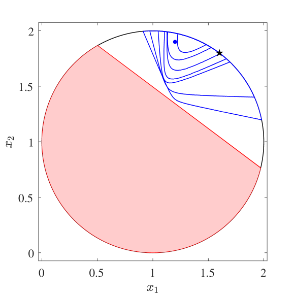
Figure 3: The blue curves depict the gradual expansion of the set of safe arms $\{x\in\mathcal{X}\ |\ \mbox{LCB}_{t}(x)\geq b\}$ over time under the SEGE algorithm for $t=250$, $500$, $1000$, $2000$, $5000$, $10000$, and $50000$. The blue dot depicts the baseline arm $X_{0}$, the black star depicts the optimal arm $X^{*}$, and the red shaded area depicts the set of unsafe arms.

6.2 Performance of the SEGE Algorithm

We first discuss the transient behavior and performance of the SEGE algorithm. As one might expect, the SEGE algorithm initially relies on the baseline arm for safe exploration as depicted in Figure 22(a). Over time, as the algorithm accumulates information, it is able to gradually expand the set of safe arms as shown in Figure 3. This expansion enables the algorithm to increase the stagewise efficiency with which it safely explores by selecting arms in the vicinity of the safe arm with the largest lower confidence bounds on their expected rewards. In turn, the SEGE algorithm is able to exploit the information gained to play the greedy with increasing frequency over time. As a result, the growth rate of regret diminishes over time as depicted in Figure 22(c). Critically, Figure 22(a) also shows that the SEGE algorithm maintains stagewise safety throughout each of the $250$ independent experiments.

6.3 Comparison with the CLUCB Algorithm

Unlike the SEGE algorithm, the CLUCB algorithm is shown to violate the stagewise safety constraint at an early stage in the learning process as depicted in Figure 22(b). The violation of the stagewise safety constraint by the CLUCB algorithm is not surprising as it is only guaranteed to respect the conservative performance constraint (6). The SEGE algorithm, on the other hand, is guaranteed to satisfy the conservative performance constraint, in addition to being stagewise safe (cf. Corollary 1). However, as one might expect, the more stringent safety guarantee of the SEGE algorithm comes at a cost. Specifically, the regret under the SEGE algorithm initially grows more rapidly than the regret incurred by the CLUCB algorithm, as shown in Figure 22(c). However, over time the growth rate of regret of the SEGE algorithm slows down as information accumulates and the need for safe exploration diminishes enabling the algorithm to play the greedy arm more frequently.

Appendix A Appendices

In this Section, we provide a detailed proof of the theoretical results including Lemma 1, and Theorems 2 and 3.

A.1 Proof of Lemma 1

Recall from the definition of $X^{\mathsf{S}}_{t}$ that $\mathbb{P}\left(\langle X^{\mathsf{S}}_{t},\theta^{*}\rangle\geq b_{0}\right)\geq 1-\delta_{t}$. Thus, with probability $1-\delta_{t}$, it holds that,

$$\langle X^{\mathsf{SE}}_{t},\theta^{*}\rangle =\langle(1-\rho)X^{\mathsf{S}}_{t}+\rho U_{t},\theta^{*}\rangle$$

$$=\langle(1-\rho)X^{\mathsf{S}}_{t}+\rho\bar{x}+\rho H^{1/2}\zeta_{t},\theta^{*}\rangle$$

$$=\langle X^{\mathsf{S}}_{t},\theta^{*}\rangle-\rho\langle X^{\mathsf{S}}_{t}-\bar{x},\theta^{*}\rangle+\rho\langle H^{1/2}\zeta_{t},\theta^{*}\rangle$$

$$\geq b_{0}-\rho\lVert X^{\mathsf{S}}_{t}-\bar{x}\rVert\lVert\theta^{*}\rVert-\rho\sqrt{\lambda_{\max}(H)}\lVert\theta^{*}\rVert,$$ (20)

where the inequality follows from the Cauchy-Schwarz inequality and the fact that $\lVert\zeta_{t}\rVert=1$. For any $x\in\mathcal{X}$, it holds that

$$\lVert x-\bar{x}\rVert \leq\lVert x-\bar{x}\rVert_{H^{-1}}\sqrt{\lambda_{\max}(H)}$$

$$\leq\sqrt{\lambda_{\max}(H)},$$ (21)

where the inequality follows from the definition of $\mathcal{X}$ in Equation (1). By applying Inequality (21) to Inequality (20), with probability $1-\delta_{t}$, it holds that

$$\langle X^{\mathsf{SE}}_{t},\theta^{*}\rangle \geq b_{0}-2\rho\sqrt{\lambda_{\max}(H)}\lVert\theta^{*}\rVert.$$

Recall Assumption 1 that $\lVert\theta^{*}\rVert\leq S$. Thus, in order to guarantee that $\mathbb{P}\left(\langle X^{\mathsf{SE}}_{t},\theta^{*}\rangle\geq b\right)\geq 1-\delta_{t}$ it suffices to choose $\rho$ such that

$$\rho\leq\frac{b_{0}-b}{2S\sqrt{\lambda_{\max}(H)}}.$$ (22)

A.2 Proof of Theorem 2

From Lemma 1, it follows that the safe exploration arm $X^{\mathsf{SE}}_{t}$ is $(\delta_{t},b)$-safe by construction. Moreover, under the SEGE algorithm the greedy arm $X^{\mathsf{CE}}_{t}$ is only played if $\mbox{LCB}_{t}(X^{\mathsf{CE}}_{t})\geq b$, which, in turn, implies

$$\mathbb{P}\left(\langle X^{\mathsf{CE}}_{t},\theta^{*}\rangle\geq b\right)\geq 1-\delta_{t}.$$

Thus, the greedy arm $X^{\mathsf{CE}}_{t}$ if played is $(\delta_{t},b)$-safe.

A.3 Proof of Theorem 3

As mentioned in the Theoretical Results section, in order to establish an upper bound on the expected regret, we rely on intermediary results. More precisely, to upper bound the expected regret during the greedy exploitation stages, we establish a bound on the stagewise regret under the greedy arm in terms of the mean squared estimation error in Lemma 2.

Lemma 2 (Stagewise Regret)

The stagewise expected reward under the greedy (certainty equivalent) arm $X^{\mathsf{CE}}_{t}$ is almost surely lower bounded as

$$\langle X^{\mathsf{CE}}_{t},\theta^{*}\rangle\geq\langle X^{*},\theta^{*}\rangle-k_{1}\left\lVert\theta^{*}-\widehat{\theta}_{t-1}\right\rVert^{2},$$ (23)

for all $t\geq 1$, where the constant $k_{1}$ is given by

$$k_{1}=\frac{2\lVert X_{0}\rVert\lambda_{\max}(H)}{b_{0}\sqrt{\lambda_{\min}(H)}}.$$

The proof of Lemma 2 is postponed to Appendix A.5.

Moreover, to upper bound the expected regret during the safe exploitation stages, we establish an upper bound on the expected number of safe exploration stages in Theorem 4. More precisely, let $N_{t}$ be the number of stages in which a safe exploration arm is played among the first $t$ stages. Then, Theorem 4 establishes an upper bound on $\mathbb{E}\left[N_{t}\right]$ under the SEGE algorithm.

Theorem 4 (Safe Exploration Stages)

Let $\{\delta_{t}\}_{t=1}^{\infty}$ be any sequence of risk levels satisfying Inequality (18) for all $t\geq 1$. There exists a finite positive constant $C_{0}$ such that under the SEGE Algorithm 1, it holds that

$$\mathbb{E}\left[N_{t}\right]\leq C_{0}\sqrt{t},$$

for all $t\geq 1$.

The proof of Lemma 4 is postponed to Appendix A.4.

Recall the definition of expected regret $R_{T}$

$$R_{T}=\mathbb{E}\left[\sum_{t=1}^{T}\langle X^{*}-X_{t},\theta^{*}\rangle\right].$$

We bound the expected regret in the exploration and exploitation stages separately. Let $\mathcal{N}_{T}^{\mathsf{SE}}$ ($\mathcal{N}_{T}^{\mathsf{CE}}$) be the stages in which a safe exploration arm (greedy arm) is played in the first $T$ stages. The expected regret can be decomposed into two parts,

$$R_{T} =\mathbb{E}\left[\sum_{t\in\mathcal{N}_{T}^{\mathsf{SE}}}\langle X^{*}-X^{\mathsf{SE}}_{t},\theta^{*}\rangle\right]+\mathbb{E}\left[\sum_{t\in\mathcal{N}_{T}^{\mathsf{CE}}}\langle X^{*}-X^{\mathsf{CE}}_{t},\theta^{*}\rangle\right].$$ (24)

The regret in safe exploration stages:  From the fact that $\lVert x\rVert\leq L$ for all $x\in\mathcal{X}$, $\lVert\theta^{*}\rVert\leq S$, and the Cauchy-Schwarz inequality it almost surely holds that

$$\sum_{t\in\mathcal{N}_{T}^{\mathsf{SE}}}\langle X^{*}-X^{\mathsf{SE}}_{t},\theta^{*}\rangle\leq 2LSN_{T}.$$

From Theorem 4, it follows that

$$\mathbb{E}\left[\sum_{t\in\mathcal{N}_{T}^{\mathsf{SE}}}\langle X^{*}-X^{\mathsf{SE}}_{t},\theta^{*}\rangle\right]\leq 2LS\mathbb{E}\left[N_{T}\right]\leq 2LSC_{0}\sqrt{T}.$$

The regret in greedy exploitation stages: Recall that the greedy arm is only played if $\mbox{LCB}_{t}(X^{\mathsf{CE}}_{t})\geq b$ and $\lambda_{\min}(V_{t})\geq c\sqrt{t}$. Notice that it almost surely holds that $\langle x,\theta^{*}\rangle\leq LS$ for all $x\in\mathcal{X}$. Then, for all $t\in\mathcal{N}_{T}^{\mathsf{CE}}$, it holds that

$$\mathbb{E}\left[\langle X^{*}-X^{\mathsf{CE}}_{t},\theta^{*}\rangle\right] =\int_{0}^{2LS}\mathbb{P}\left(\left\{\langle X^{*}-X^{\mathsf{CE}}_{t},\theta^{*}\rangle\geq\gamma\right\}\bigcap\left\{\lambda_{\min}(V_{t-1})\geq c\sqrt{t}\right\}\bigcap\left\{\mbox{LCB}_{t}(X^{\mathsf{CE}}_{t})\geq b\right\}\right)\ d\gamma$$

$$\leq\int_{0}^{2LS}\mathbb{P}\left(\left\{\langle X^{*}-X^{\mathsf{CE}}_{t},\theta^{*}\rangle\geq\gamma\right\}\bigcap\left\{\lambda_{\min}(V_{t-1})\geq c\sqrt{t}\right\}\right)\ d\gamma$$

$$\leq\int_{0}^{2LS}\mathbb{P}\left(\left\{k_{1}\lVert\theta^{*}-\widehat{\theta}_{t-1}\rVert^{2}\geq\gamma\right\}\bigcap\left\{\lambda_{\min}(V_{t-1})\geq c\sqrt{t}\right\}\right)\ d\gamma,$$

where the last inequality follows from the bound on the stagewise regret in Inequality (23). From the Cauchy-Schwarz inequality it follows that $\lVert\theta^{*}-\widehat{\theta}_{t-1}\rVert_{V_{t-1}}\geq\lVert\theta^{*}-\widehat{\theta}_{t-1}\rVert\sqrt{\lambda_{\min}(V_{t-1})}$. Then,

$$\mathbb{E}\left[\langle X^{*}-X^{\mathsf{CE}}_{t},\theta^{*}\rangle\right] \leq\int_{0}^{2LS}\mathbb{P}\left(\left\{\lVert\theta^{*}-\widehat{\theta}_{t-1}\rVert^{2}_{V_{t-1}}\geq\frac{\gamma c\sqrt{t}}{k_{1}}\right\}\bigcap\left\{\lambda_{\min}(V_{t-1})\geq c\sqrt{t}\right\}\right)\ d\gamma$$

$$\leq\int_{0}^{2LS}\mathbb{P}\left(\lVert\theta^{*}-\widehat{\theta}_{t-1}\rVert^{2}_{V_{t-1}}\geq\frac{\gamma c\sqrt{t}}{k_{1}}\right)\ d\gamma$$

$$\leq\gamma_{t-1}+\int_{\gamma_{t-1}}^{2LS}\mathbb{P}\left(\lVert\theta^{*}-\widehat{\theta}_{t-1}\rVert^{2}_{V_{t-1}}\geq\frac{\gamma c\sqrt{t}}{k_{1}}\right)\ d\gamma,$$ (25)

where the last inequality follows from upper bounding the integrand by $1$ for $\gamma\leq\gamma_{t-1}$. Here, $\gamma_{t-1}$ is defined as

$$\gamma_{t-1}=k_{7}\frac{\log\left(t\right)}{\sqrt{t}},$$ (26)

where $k_{4}$ is defined as

$$k_{7}=\frac{2k_{1}d\sigma_{\eta}^{2}}{c}\left(\log(1+L^{2}/\lambda)+\frac{2\lambda S^{2}}{d\sigma_{\eta}^{2}}\right).$$ (27)

Recall from the definition of $\mathcal{C}_{t-1}(\delta)$ that for any $\delta\in(0,1)$, it holds that

$$\mathbb{P}\left(\lVert\theta^{*}-\widehat{\theta}_{t-1}\rVert_{V_{t-1}}\geq r_{t}(\delta)\right)\leq\delta.$$ (28)

In order to apply Inequality (28) to (25), we set $\delta$ such that $r_{t}^{2}(\delta)=c\sqrt{t}\gamma/k_{1}$, i.e.,

$$\delta=(1+tL^{2}/\lambda)\exp\left(-\frac{1}{d\sigma_{\eta}^{2}}\left(\sqrt{\frac{c\sqrt{t}\gamma}{k_{1}}}-\sqrt{\lambda}S\right)^{2}\right).$$

Using the fact that for any two real numbers $x,y>0$, we have that $(\sqrt{x}-\sqrt{y})^{2}\geq x/2-y$, we get

$$\delta\leq(1+tL^{2}/\lambda)\exp\left(\frac{2\lambda S^{2}}{d\sigma_{\eta}^{2}}\right)\exp\left(-\frac{c\gamma}{2k_{1}d\sigma_{\eta}^{2}}\sqrt{t}\right).$$ (29)

Then, by applying Inequality (28) and (29) to Inequality (25), we get

$$\mathbb{E}\left[\langle X^{*}-X^{\mathsf{CE}}_{t},\theta^{*}\rangle\right] \leq\gamma_{t-1}+(1+tL^{2}/\lambda)\exp\left(\frac{2\lambda S^{2}}{d\sigma_{\eta}^{2}}\right)\int_{\gamma_{t-1}}^{2LS}\exp\left(-\frac{c\gamma}{2k_{1}d\sigma_{\eta}^{2}}\sqrt{t}\right)\ d\gamma$$

$$\leq\gamma_{t-1}+(1+tL^{2}/\lambda)\exp\left(\frac{2\lambda S^{2}}{d\sigma_{\eta}^{2}}\right)\exp\left(-\frac{c\gamma_{t-1}}{2k_{1}d\sigma_{\eta}^{2}}\sqrt{t}\right)\frac{2k_{1}d\sigma_{\eta}^{2}}{c\gamma\sqrt{t}}$$

$$\leq\gamma_{t-1}+\frac{2k_{1}d\sigma_{\eta}^{2}}{c\sqrt{t}},$$ (30)

where the last inequality follows from the fact that $(1+tL^{2}/\lambda)\exp\left(\frac{2\lambda S^{2}}{d\sigma_{\eta}^{2}}\right)\exp\left(-\frac{c\gamma_{t-1}}{2k_{1}d\sigma_{\eta}^{2}}\sqrt{t}\right)\leq 1$ by definition, i.e.,

$$(1+tL^{2}/\lambda)\exp\left(\frac{2\lambda S^{2}}{d\sigma_{\eta}^{2}}\right)\exp\left(-\frac{c\gamma_{t-1}}{2k_{1}d\sigma_{\eta}^{2}}\sqrt{t}\right) \leq t(1+L^{2}/\lambda)\exp\left(\frac{2\lambda S^{2}}{d\sigma_{\eta}^{2}}\right)\exp\left(-\frac{ck_{7}\log(t)}{2k_{1}d\sigma_{\eta}^{2}}\right)$$

$$=(1+L^{2}/\lambda)\exp\left(\frac{2\lambda S^{2}}{d\sigma_{\eta}^{2}}\right)\exp\left(-\frac{ck_{7}}{2k_{1}d\sigma_{\eta}^{2}}\right)$$

$$=1,$$

where the last inequality follows from the definition of $k_{7}$ in inequality (27). Thus, using Inequality (30) and the definition of $\gamma_{t-1}$ in (26), we get

$$\mathbb{E}\left[\sum_{t\in\mathcal{N}_{T}^{\mathsf{CE}}}\langle X^{*}-X^{\mathsf{CE}}_{t},\theta^{*}\rangle\right] \leq\sum_{t=2}^{T}\left(k_{7}\frac{\log\left(t\right)}{\sqrt{t}}+\frac{2k_{1}d\sigma_{\eta}^{2}}{c\sqrt{t}}\right)$$

$$\leq\sum_{t=2}^{T}\left(k_{7}\frac{\log(T)}{\sqrt{t}}+\frac{2k_{1}d\sigma_{\eta}^{2}}{c\sqrt{t}}\right)$$

$$\leq\left(k_{7}\log(T)+\frac{2k_{1}d\sigma_{\eta}^{2}}{c}\right)\int_{t=1}^{T}\frac{1}{\sqrt{t}}\ dt$$

$$\leq C_{0}\sqrt{T}+C_{1}\sqrt{T}\log(T),$$

where $C_{2}$ and $C_{3}$ are defined as

$$C_{2} =\frac{4k_{1}d\sigma_{\eta}^{2}}{c},$$

$$C_{3} =2k_{7}.$$

Thus, by defining $C=2LSC_{0}+C_{2}+C_{3}$, we get the desired upper bound on regret.

A.4 Proof of Theorem 4

From the definition of $N_{t}$, it follows that $N_{0}=0$ and for all $t\geq 0$,

$$N_{t+1}=\begin{cases}N_{t},&\lambda_{\min}(V_{t})\geq c\sqrt{t}\ \text{and}\ \mbox{LCB}_{t}(X^{\mathsf{CE}}_{t})\geq b,\\ N_{t}+1,&\text{otherwise}.\end{cases}$$ (31)

Fix $\mu\in(0,1)$. Define the random process $\{Z\}_{t=1}^{\infty}$ as follows. For any $t\geq 0$, $Z_{t}$ is defined as

$$Z_{t}=0\vee\left(N_{t}-\left\lceil\frac{c\sqrt{t}}{\mu\rho^{2}\sigma^{2}}\right\rceil\right).$$ (32)

Notice that if $N_{t}<\left\lceil\frac{c\sqrt{t}}{\mu\rho^{2}\sigma^{2}}\right\rceil$ then $Z_{t+1}=0$. Thus,

$$\mathbb{E}\left[Z_{t+1}\right] =\mathbb{E}\left[Z_{t}\right]+\mathbb{E}\left[\mathds{1}\left\{\left\{N_{t}\geq\left\lceil\frac{c\sqrt{t}}{\mu\rho^{2}\sigma^{2}}\right\rceil\right\}\cap\left(\left\{\lambda_{\min}(V_{t})\leq c\sqrt{t}\right\}\cup\left\{{{\mbox{LCB}}_{t}}(X^{\mathsf{CE}}_{t})\leq b\right\}\right)\right\}\right]$$

$$=\mathbb{E}\left[Z_{t}\right]+\mathbb{P}\left(\left\{N_{t}\geq\left\lceil\frac{c\sqrt{t}}{\mu\rho^{2}\sigma^{2}}\right\rceil\right\}\cap\left(\left\{\lambda_{\min}(V_{t})\leq c\sqrt{t}\right\}\cup\left\{{{\mbox{LCB}}_{t}}(X^{\mathsf{CE}}_{t})\leq b\right\}\right)\right)$$

$$=\sum_{k=1}^{t}\mathbb{P}\left(\left\{N_{k}\geq\left\lceil\frac{c\sqrt{k}}{\mu\rho^{2}\sigma^{2}}\right\rceil\right\}\cap\left(\left\{\lambda_{\min}(V_{k})\leq c\sqrt{k}\right\}\cup\left\{{{\mbox{LCB}}_{k}}(X^{\mathsf{CE}}_{k})\leq b\right\}\right)\right)$$ (33)

To establish an upper bound on the probability of the events in Equation (33), we establish the following relationship.

Lemma 3

Conditioned on the event $\lambda_{\min}(V_{t})\geq c\sqrt{t}$, we have that $\theta^{*}\in\mathcal{C}_{t-1}\left(\delta_{t}\wedge\widehat{\delta}_{t}\right)$ implies ${{\mbox{LCB}}_{t}}(X^{\mathsf{CE}}_{t})\geq b$, i.e.,

$$\left\{\lambda_{\min}(V_{t})\geq c\sqrt{t}\right\}\cap\left\{\theta^{*}\in\mathcal{C}_{t-1}\left(\delta_{t}\wedge\widehat{\delta}_{t}\right)\right\}\subseteq\left\{\lambda_{\min}(V_{t})\geq c\sqrt{t}\right\}\cap\left\{{{\mbox{LCB}}_{t}}(X^{\mathsf{CE}}_{t})\geq b\right\}.$$

Here, $\widehat{\delta}_{t}$ is defined as

$$\widehat{\delta}_{t}=\left(1+\frac{tL^{2}}{\lambda}\right)\exp\left(-\frac{k_{2}c\sqrt{t}-2\lambda S^{2}}{2\sigma_{\eta}^{2}d}\right),$$

where the positive constant $k_{2}$ is defined as

$$k_{2}=\left(\sqrt{\frac{b_{0}-b}{k_{1}}+\frac{L^{2}}{k_{1}^{2}}}-\frac{L}{k_{1}}\right)^{2}$$

By applying De Morgan’s law and Lemma 3 to Inequality (33), we get

$$\mathbb{E}\left[Z_{t+1}\right] \leq\sum_{k=1}^{t}\mathbb{P}\left(\left\{N_{k}\geq\left\lceil\frac{c\sqrt{k}}{\mu\rho^{2}\sigma^{2}}\right\rceil\right\}\cap\left(\left\{\lambda_{\min}(V_{k})\leq c\sqrt{k}\right\}\cup\left\{\theta^{*}\notin\mathcal{C}_{k-1}\left(\delta_{k}\wedge\widehat{\delta}_{k}\right)\right\}\right)\right)$$

$$\leq\sum_{k=1}^{t}\mathbb{P}\left(\left\{N_{k}\geq\left\lceil\frac{c\sqrt{k}}{\mu\rho^{2}\sigma^{2}}\right\rceil\right\}\cap\left\{\lambda_{\min}(V_{k})\leq c\sqrt{k}\right\}\right)+\mathbb{P}\left(\theta^{*}\notin\mathcal{C}_{k-1}\left(\delta_{k}\wedge\widehat{\delta}_{k}\right)\right)$$

$$\leq\sum_{k=1}^{t}\mathbb{P}\left(\left\{N_{k}\geq\left\lceil\frac{c\sqrt{k}}{\mu\rho^{2}\sigma^{2}}\right\rceil\right\}\cap\left\{\lambda_{\min}(V_{k})\leq c\sqrt{k}\right\}\right)+\delta_{k}\wedge\widehat{\delta}_{k}$$

$$\leq\sum_{k=1}^{t}\mathbb{P}\left(\left\{N_{k}\geq\left\lceil\frac{c\sqrt{k}}{\mu\rho^{2}\sigma^{2}}\right\rceil\right\}\cap\left\{\lambda_{\min}(V_{k})\leq c\sqrt{k}\right\}\right)+\widehat{\delta}_{k}.$$

Using the total probability theorem, we have that

$$\mathbb{P}\left(\left\{N_{k}\geq\left\lceil\frac{c\sqrt{k}}{\mu\rho^{2}\sigma^{2}}\right\rceil\right\}\cap\left\{\lambda_{\min}(V_{k})\leq c\sqrt{k}\right\}\right) =\sum_{n=\left\lceil\frac{c\sqrt{k}}{\mu\rho^{2}\sigma^{2}}\right\rceil}^{\infty}\mathbb{P}\left(\lambda_{\min}(V_{k})\leq c\sqrt{k}\mid N_{k}=n\right)\mathbb{P}\left(N_{k}=n\right)$$

$$\leq\sum_{n=\left\lceil\frac{c\sqrt{k}}{\mu\rho^{2}\sigma^{2}}\right\rceil}^{\infty}\mathbb{P}\left(\lambda_{\min}(V_{k})\leq\mu\rho^{2}\sigma^{2}N_{k}\mid N_{k}=n\right)\mathbb{P}\left(N_{k}=n\right).$$ (34)

We now establish an upper bound on the minimum eigenvalue of $V_{t}$ in terms of the number of safe exploration stages.

Lemma 4 (Random Exploration)

Under the SEGE Algorithm, for any $\mu\in(0,1)$ it holds that

$$\mathbb{P}\left(\lambda_{\min}(V_{t})\leq\mu\rho^{2}\sigma^{2}N_{t}\mid N_{t}=n\right)\leq de^{-k_{4}(1-\mu)^{2}n},$$ (35)

where $c_{1}$ is defined as

$$k_{4} =\frac{\rho^{4}\sigma^{4}}{2k_{3}^{2}},$$

$$k_{3} =2\rho((1-\rho)L+\rho\lVert\bar{x}\rVert)\sqrt{\lambda_{\max}(H)}+\rho^{2}\lambda_{\max}(H)-\rho^{2}\sigma^{2}d.$$

By applying Inequality (35) to Inequality (34), we

$$\mathbb{P}\left(\left\{N_{k}\geq\left\lceil\frac{c\sqrt{k}}{\mu\rho^{2}\sigma^{2}}\right\rceil\right\}\cap\left\{\lambda_{\min}(V_{k})\leq c\sqrt{k}\right\}\right) \leq\sum_{n=\left\lceil\frac{c\sqrt{k}}{\mu\rho^{2}\sigma^{2}}\right\rceil}^{\infty}d\exp\left(-k_{4}(1-\mu)^{2}n\right)\mathbb{P}\left(N_{k}=n\right)$$

$$\leq d\exp\left(-\frac{k_{4}(1-\mu)^{2}c}{\mu\rho^{2}\sigma^{2}}\sqrt{k}\right)\sum_{n=\left\lceil\frac{c\sqrt{k}}{\mu\rho^{2}\sigma^{2}}\right\rceil}^{\infty}\mathbb{P}\left(N_{k}=n\right)$$

$$\leq d\exp\left(-\frac{k_{4}(1-\mu)^{2}c}{\mu\rho^{2}\sigma^{2}}\sqrt{k}\right).$$

Thus,

$$\mathbb{E}\left[Z_{t}\right] \leq\sum_{k=1}^{t-1}\left(d\exp\left(-\frac{k_{4}(1-\mu)^{2}c}{\mu\rho^{2}\sigma^{2}}\sqrt{k}\right)+\left(1+\frac{kL^{2}}{\lambda}\right)\exp\left(-\frac{k_{2}c\sqrt{k}-2\lambda S^{2}}{2\sigma_{\eta}^{2}d}\right)\right)$$

$$\leq\sum_{k=1}^{t-1}\left(d\exp\left(-\frac{k_{4}(1-\mu)^{2}c}{\mu\rho^{2}\sigma^{2}}\sqrt{k}\right)+k_{5}k\exp\left(-\frac{k_{2}c}{2\sigma_{\eta}^{2}d}\sqrt{k}\right)\right),$$

where $k_{5}$ is defined as

$$k_{5}=\left(1+\frac{L^{2}}{\lambda}\right)\exp\left(\frac{\lambda S^{2}}{\sigma_{\eta}^{2}d}\right).$$

Then,

$$\mathbb{E}\left[Z_{t}\right] \leq d\int_{0}^{t}\exp\left(-\frac{k_{4}(1-\mu)^{2}c}{\mu\rho^{2}\sigma^{2}}\sqrt{x}\right)\ dx+k_{5}\int_{0}^{t}x\exp\left(-\frac{k_{2}c}{2\sigma_{\eta}^{2}d}\sqrt{x}\right)\ dx$$

$$\leq d\int_{0}^{\infty}\exp\left(-\frac{k_{4}(1-\mu)^{2}c}{\mu\rho^{2}\sigma^{2}}\sqrt{x}\right)\ dx+k_{5}\int_{0}^{\infty}x\exp\left(-\frac{k_{2}c}{2\sigma_{\eta}^{2}d}\sqrt{x}\right)\ dx$$

$$=-d\frac{2(\mu\rho^{2}\sigma^{2})^{2}}{(k_{4}(1-\mu)^{2}c)^{2}}\exp\left(-\frac{k_{4}(1-\mu)^{2}c}{\mu\rho^{2}\sigma^{2}}\sqrt{x}\right)\left(\frac{k_{4}(1-\mu)^{2}c}{\mu\rho^{2}\sigma^{2}}\sqrt{x}+1\right)\bigg{|}_{0}^{\infty}$$

$$\qquad-\frac{2(2\sigma_{\eta}^{2}d)^{4}}{(k_{2}c)^{4}}\exp\left(-\frac{k_{2}c}{2\sigma_{\eta}^{2}d}\sqrt{x}\right)\left(\left(\frac{k_{2}c}{2\sigma_{\eta}^{2}d}\right)^{3}x^{3/2}+3\left(\frac{k_{2}c}{2\sigma_{\eta}^{2}d}\right)^{2}x+6\frac{k_{2}c}{2\sigma_{\eta}^{2}d}\sqrt{x}+6\right)\bigg{|}_{0}^{\infty}$$

$$=k_{6},$$

where $k_{6}$ is defined as

$$k_{6} =d\frac{2(\mu\rho^{2}\sigma^{2})^{2}}{(k_{4}(1-\mu)^{2}c)^{2}}+k_{5}\frac{12(2\sigma_{\eta}^{2}d)^{4}}{(k_{2}c)^{4}}.$$

Thus,

$$\mathbb{E}\left[N_{t}\right] \leq\mathbb{E}\left[Z_{t}\right]+\left\lceil\frac{c\sqrt{t}}{\mu\rho^{2}\sigma^{2}}\right\rceil$$

$$\leq k_{6}+1+\frac{c\sqrt{t}}{\mu\rho^{2}\sigma^{2}}.$$

Setting $C_{0}=k_{6}+1+\frac{c}{\mu\rho^{2}\sigma^{2}}$ concludes the proof.

A.5 Proof of Lemma 2

For each $t\geq 1$, the expected reward under the greedy arm is lower bounded as

$$\langle X^{\mathsf{CE}}_{t},\theta^{*}\rangle =\langle X^{*},\theta^{*}\rangle-\langle X^{*}-X^{\mathsf{CE}}_{t},\theta^{*}\rangle$$

$$=\langle X^{*},\theta^{*}\rangle-\langle X^{*}-X^{\mathsf{CE}}_{t},\theta^{*}-\widehat{\theta}_{t-1}\rangle-\langle X^{*}-X^{\mathsf{CE}}_{t},\widehat{\theta}_{t-1}\rangle$$

$$\geq\langle X^{*},\theta^{*}\rangle-\langle X^{*}-X^{\mathsf{CE}}_{t},\theta^{*}-\widehat{\theta}_{t-1}\rangle,$$

where the inequality follows from the fact that $\langle X^{\mathsf{CE}}_{t},\widehat{\theta}_{t-1}\rangle\geq\langle x,\widehat{\theta}_{t-1}\rangle$ for all $x\in\mathcal{X}$ as the greedy arm is the optimal arm for the reward parameter $\widehat{\theta}_{t-1}$. Using the Cauchy-Schwarz inequality, we get

$$\langle X^{\mathsf{CE}}_{t},\theta^{*}\rangle \geq\langle X^{*},\theta^{*}\rangle-\lVert X^{*}-X^{\mathsf{CE}}_{t}\rVert\lVert\theta^{*}-\widehat{\theta}_{t-1}\rVert$$

$$=\langle X^{*},\theta^{*}\rangle-\left\lVert\frac{H\theta^{*}}{\lVert\theta^{*}\rVert_{H}}-\dfrac{H\widehat{\theta}_{t-1}}{\lVert\widehat{\theta}_{t-1}\rVert_{H}}\right\rVert\lVert\theta^{*}-\widehat{\theta}_{t-1}\rVert.$$ (36)

We now show that

$$\left\lVert\frac{H\theta^{*}}{\lVert\theta^{*}\rVert_{H}}-\dfrac{H\widehat{\theta}_{t-1}}{\lVert\widehat{\theta}_{t-1}\rVert_{H}}\right\rVert\leq\frac{2\lVert X_{0}\rVert{\lambda_{\max}(H)}}{b_{0}\sqrt{\lambda_{\min}(H)}}\lVert\theta^{*}-\widehat{\theta}_{t-1}\rVert.$$ (37)

Using the triangle inequality, we get

$$\left\lVert\frac{H\theta^{*}}{\lVert\theta^{*}\rVert_{H}}-\dfrac{H\widehat{\theta}_{t-1}}{\lVert\widehat{\theta}_{t-1}\rVert_{H}}\right\rVert =\left\lVert\frac{H\theta^{*}}{\lVert\theta^{*}\rVert_{H}}-\frac{H\widehat{\theta}_{t-1}}{\lVert\theta^{*}\rVert_{H}}+\frac{H\widehat{\theta}_{t-1}}{\lVert\theta^{*}\rVert_{H}}-\dfrac{H\widehat{\theta}_{t-1}}{\lVert\widehat{\theta}_{t-1}\rVert_{H}}\right\rVert$$

$$\leq\left\lVert\frac{H\theta^{*}}{\lVert\theta^{*}\rVert_{H}}-\frac{H\widehat{\theta}_{t-1}}{\lVert\theta^{*}\rVert_{H}}\right\rVert+\left\lVert\frac{H\widehat{\theta}_{t-1}}{\lVert\theta^{*}\rVert_{H}}-\dfrac{H\widehat{\theta}_{t-1}}{\lVert\widehat{\theta}_{t-1}\rVert_{H}}\right\rVert$$

$$=\frac{1}{\lVert\theta^{*}\rVert_{H}}\lVert H(\theta^{*}-\widehat{\theta}_{t-1})\rVert+\frac{\lVert H\widehat{\theta}_{t-1}\rVert}{\lVert\theta^{*}\rVert_{H}\lVert\widehat{\theta}_{t-1}\rVert_{H}}\left|\lVert\theta^{*}\rVert_{H}-\lVert\widehat{\theta}_{t-1}\rVert_{H}\right|$$

$$\leq\frac{1}{\lVert\theta^{*}\rVert_{H}}\lVert H(\theta^{*}-\widehat{\theta}_{t-1})\rVert+\frac{\lVert H\widehat{\theta}_{t-1}\rVert}{\lVert\theta^{*}\rVert_{H}\lVert\widehat{\theta}_{t-1}\rVert_{H}}\lVert\theta^{*}-\widehat{\theta}_{t-1}\rVert_{H},$$

where the last inequality follows from the reverse triangle inequality. Using the Cauchy-Schwarz inequality and the fact that $\lVert H\rVert=\lambda_{\max}(H)$, we get

$$\frac{1}{\lVert\theta^{*}\rVert_{H}}\lVert H(\theta^{*}-\widehat{\theta}_{t-1})\rVert+\frac{\lVert H\widehat{\theta}_{t-1}\rVert}{\lVert\theta^{*}\rVert_{H}\lVert\widehat{\theta}_{t-1}\rVert_{H}}\lVert\theta^{*}-\widehat{\theta}_{t-1}\rVert_{H}$$

$$\leq\frac{\lambda_{\max}(H)}{\lVert\theta^{*}\rVert_{H}}\lVert\theta^{*}-\widehat{\theta}_{t-1}\rVert+\frac{\sqrt{\lambda_{\max}(H)}\lVert\widehat{\theta}_{t-1}\rVert_{H}}{\lVert\theta^{*}\rVert_{H}\lVert\widehat{\theta}_{t-1}\rVert_{H}}\sqrt{\lambda_{\max}(H)}\lVert\theta^{*}-\widehat{\theta}_{t-1}\rVert$$

$$=\frac{2\lambda_{\max}(H)}{\lVert\theta^{*}\rVert_{H}}\lVert\theta^{*}-\widehat{\theta}_{t-1}\rVert,$$ (38)

where the inequality follows from the fact that $\lVert H\widehat{\theta}_{t-1}\rVert\leq\lVert H^{1/2}\rVert\lVert H^{1/2}\widehat{\theta}_{t-1}\rVert=\sqrt{\lambda_{\max}(H)}\lVert\widehat{\theta}_{t-1}\rVert_{H}$. Recall from Assumption 3 that $\langle X_{0},\theta^{*}\rangle\geq b_{0}$. So, $\lVert X_{0}\rVert\lVert\theta^{*}\rVert\geq b_{0}$

$$\lVert\theta^{*}\rVert_{H}\geq\frac{\sqrt{\lambda_{\min}(H)}b_{0}}{\lVert X_{0}\rVert}.$$ (39)

Thus, by applying Inequality (39) to (38), we get Inequality (37). Finally, combining Inequalities (36) and (37) yields the desired lower bound on the expected reward of the greedy arm.

A.6 Proof of Lemma 3

For $x\in\mathcal{X}$, let $\widehat{\mbox{LCB}}_{t}(x)$ be the lower confidence bound on the reward of arm $x$ computed using the confidence set $\mathcal{C}_{t-1}(\widehat{\delta}_{t})$, i.e.,

$$\widehat{\mbox{LCB}}_{t}(x)=\langle x,\widehat{\theta}_{t-1}\rangle-r_{t}(\widehat{\delta}_{t})\lVert x\rVert_{V_{t-1}^{-1}}.$$

Notice that for any $\delta,\widehat{\delta}\in(0,1)$ the condition $\widehat{\delta}\leq\delta$ implies that $r_{t}(\widehat{\delta})\geq r_{t}(\delta)$. Thus, if $\widehat{\delta}_{t}\leq\delta_{t}$ then $\widehat{\mbox{LCB}}_{t}(x)\leq\mbox{LCB}_{t}(x)$.

Recall that $\theta^{*}\in\mathcal{C}_{t-1}(\delta_{t})$ implies that ${{\mbox{LCB}}_{t}}(X^{\mathsf{CE}}_{t})\geq b$. Thus, to prove the Lemma it suffices to show that given $\lambda_{\min}(V_{t})\geq c\sqrt{t}$ and $\theta^{*}\in\mathcal{C}_{t-1}(\widehat{\delta}_{t})$ , we have that $\widehat{\mbox{LCB}}_{t}(X^{\mathsf{CE}}_{t})\geq b$. It holds that

$$\widehat{\mbox{LCB}}_{t}(X^{\mathsf{CE}}_{t}) =\langle X^{\mathsf{CE}}_{t},\widehat{\theta}_{t-1}\rangle-r_{t}(\widehat{\delta}_{t})\left\lVert X^{\mathsf{CE}}_{t}\right\rVert_{V_{t-1}^{-1}}$$

$$\geq\langle X^{\mathsf{CE}}_{t},\theta^{*}\rangle-2r_{t}(\widehat{\delta}_{t})\left\lVert X^{\mathsf{CE}}_{t}\right\rVert_{V_{t-1}^{-1}}$$

$$\geq\langle X^{*},\theta^{*}\rangle-k_{1}\left\lVert\theta^{*}-\widehat{\theta}_{t-1}\right\rVert^{2}-2r_{t}(\widehat{\delta}_{t})\left\lVert X^{\mathsf{CE}}_{t}\right\rVert_{V_{t-1}^{-1}},$$

where the first inequality follows from the fact that $\lVert\theta^{*}-\widehat{\theta}_{t-1}\rVert_{V_{t-1}}\leq r_{t}(\widehat{\delta}_{t})$ and the second inequality follows from Lemma 2. Then, using the fact that $\langle X^{*},\theta^{*}\rangle\geq b_{0}$ we get

$$\widehat{\mbox{LCB}}_{t}(X^{\mathsf{CE}}_{t}) \geq b_{0}-k_{1}\left\lVert\theta^{*}-\widehat{\theta}_{t-1}\right\rVert^{2}-2r_{t}(\widehat{\delta}_{t})\left\lVert X^{\mathsf{CE}}_{t}\right\rVert_{V_{t-1}^{-1}}$$

$$\geq b_{0}-\frac{k_{1}}{\lambda_{\min}(V_{t-1})}\left\lVert\theta^{*}-\widehat{\theta}_{t-1}\right\rVert^{2}_{V_{t-1}}-2r_{t}(\widehat{\delta}_{t})\left\lVert X^{\mathsf{CE}}_{t}\right\rVert_{V_{t-1}^{-1}}$$

$$\geq b_{0}-k_{1}\frac{r_{t}(\widehat{\delta}_{t})^{2}}{\lambda_{\min}(V_{t-1})}-2L\frac{r_{t}(\widehat{\delta}_{t})}{\sqrt{\lambda_{\min}(V_{t-1})}}$$

$$\geq b_{0}-k_{1}\frac{r_{t}(\widehat{\delta}_{t})^{2}}{\lambda_{\min}(V_{t-1})}-2L\frac{r_{t}(\widehat{\delta}_{t})}{\sqrt{\lambda_{\min}(V_{t-1})}}$$

$$=b_{0}+\frac{L^{2}}{k_{1}}-k_{1}\left(\frac{r_{t}(\widehat{\delta}_{t})}{\sqrt{\lambda_{\min}(V_{t-1})}}+\frac{L}{k_{1}}\right)^{2}$$

$$\geq b_{0}+\frac{L^{2}}{k_{1}}-k_{1}\left(\frac{r_{t}(\widehat{\delta}_{t})}{\sqrt{c\sqrt{t}}}+\frac{L}{k_{1}}\right)^{2}.$$

In order to show that $\widehat{\mbox{LCB}}_{t}(X^{\mathsf{CE}}_{t})\geq b$, it suffices to show that

$$b_{0}+\frac{L^{2}}{k_{1}}-k_{1}\left(\frac{r_{t}(\widehat{\delta}_{t})}{\sqrt{c\sqrt{t}}}+\frac{L}{k_{1}}\right)^{2}\geq b,$$

or equivalently

$$r_{t}(\widehat{\delta}_{t})^{2}\leq\left(\sqrt{\frac{b_{0}-b}{k_{1}}+\frac{L^{2}}{k_{1}^{2}}}-\frac{L}{k_{1}}\right)^{2}c\sqrt{t}.$$

It holds that

$$r_{t}(\delta)^{2}\leq 2\sigma_{\eta}^{2}d\log\left(\frac{1+tL^{2}/\lambda}{\delta}\right)+2\lambda S^{2}.$$

From the definition of $\widehat{\delta}_{t}$ it immediately follows that

$$2\sigma_{\eta}^{2}d\log\left(\frac{1+tL^{2}/\lambda}{\widehat{\delta}_{t}}\right)+2\lambda S^{2}=\left(\sqrt{\frac{b_{0}-b}{k_{1}}+\frac{L^{2}}{k_{1}^{2}}}-\frac{L}{k_{1}}\right)^{2}c\sqrt{t}.$$

Thus, if $\widehat{\delta}_{t}\leq\delta_{t}$ then $\mbox{LCB}_{t}(X^{\mathsf{CE}}_{t})\geq b$.

A.7 Proof of Lemma 4

Let $\mathcal{N}_{t}^{\mathsf{SE}}$ be the set of stages in which a safe exploration arm is played up to and including stage $t$. Our objective is to establish a lower bound on the minimum eigenvalue of $V_{t}$ in terms on $N_{t}$. As $yy^{\top}$ is a positive semidefinite matrix for any $y\in\mathbb{R}^{d}$, it holds that

$$V_{t} =\lambda I+\sum_{k=1}^{t}X_{t}X_{t}^{\top}$$

$$\succeq\sum_{k\in\mathcal{N}_{t}^{\mathsf{SE}}}X^{\mathsf{SE}}_{k}{X^{\mathsf{SE}}_{k}}^{\top}$$

$$=\sum_{k\in\mathcal{N}_{t}^{\mathsf{SE}}}\bigg{(}((1-\rho)X^{\mathsf{S}}_{k}+\rho\bar{x}+\rho H^{1/2}\zeta_{k})((1-\rho)X^{\mathsf{S}}_{k}+\rho\bar{x}+\rho H^{1/2}\zeta_{k})^{\top}\bigg{)}$$

$$\succeq\sum_{k\in\mathcal{N}_{t}^{\mathsf{SE}}}\bigg{(}((1-\rho)X^{\mathsf{S}}_{k}+\rho\bar{x})(\rho H^{1/2}\zeta_{k})^{\top}+\rho H^{1/2}\zeta_{k}((1-\rho)X^{\mathsf{S}}_{k}+\rho\bar{x})^{\top}+\rho^{2}H^{1/2}\zeta_{k}\zeta_{k}^{\top}H^{1/2}\bigg{)}$$

$$=\sum_{k\in\mathcal{N}_{t}^{\mathsf{SE}}}\left(\rho^{2}H^{1/2}\mathbb{E}\left[\zeta_{k}\zeta_{k}^{\top}\right]H^{1/2}+W_{k}\right)$$

$$\succeq\sum_{k\in\mathcal{N}_{t}^{\mathsf{SE}}}\left(\rho^{2}\lambda_{\min}\left(H^{1/2}\mathbb{E}\left[\zeta_{k}\zeta_{k}^{\top}\right]H^{1/2}\right)+W_{k}\right),$$

where $W_{k}$ is defined as

$$W_{k}= ((1-\rho)X^{\mathsf{S}}_{k}+\rho\bar{x})(\rho H^{1/2}\zeta_{k})^{\top}+\rho H^{1/2}\zeta_{k}((1-\rho)X^{\mathsf{S}}_{k}+\rho\bar{x})^{\top}+\rho^{2}H^{1/2}(\zeta_{k}\zeta_{k}^{\top}-\mathbb{E}\left[\zeta_{k}\zeta_{k}^{\top}\right])H^{1/2}.$$ (40)

Recall that $\sigma^{2}$ is defined as the minimum eigenvalue of the covariance matrix of $U_{k}$, i.e.,

$$\sigma^{2} =\lambda_{\min}\left(\mathbb{E}\left[\left(U_{k}-\mathbb{E}\left[U_{k}\right]\right)\left(U_{k}-\mathbb{E}\left[U_{k}\right]\right)^{\top}\right]\right)$$

$$=\lambda_{\min}\left(H^{1/2}\mathbb{E}\left[\zeta_{k}\zeta_{k}^{\top}\right]H^{1/2}\right).$$

Thus, using the fact that $|\mathcal{N}_{t}^{\mathsf{SE}}|=N_{t}$, we get

$$V_{t} \succeq\rho^{2}\sigma^{2}N_{t}I+\sum_{k\in\mathcal{N}_{t}^{\mathsf{SE}}}W_{k}.$$

Using Weyl’s inequality, it immediately follows that

$$\lambda_{\min}(V_{t})\geq\rho^{2}\sigma^{2}N_{t}-\lambda_{\max}\left(\sum_{k\in\mathcal{N}_{t}^{\mathsf{SE}}}W_{k}\right).$$ (41)

We rely on the Matrix Azuma Inequality (42) to establish an upper bound on $\lambda_{\max}(\sum_{k\in\mathcal{N}_{t}}W_{k})$, which holds with high probability.

Theorem 5 (Matrix Azuma Inequality)

(?, Theorem 7.1. and Remark 7.8.) Let $\{\mathcal{F}_{k}\}_{k=0}^{\infty}$ be a filtration. Consider the random process $\{Y_{k}\}_{k=1}^{\infty}$ adapted to the filtration $\{\mathcal{F}_{k}\}_{k=1}^{\infty}$. Each $Y_{k}$ is a self-adjoint matrix with dimension $d$ such that

$$\mathbb{E}\left[Y_{k}\mid\mathcal{F}_{k-1}\right]=0\ \text{for}\ k=1,2,3,\ldots.,$$

and

$$Y_{k}^{2}\preceq A_{k}^{2}\ \text{almost surely for}\ k=1,2,3,\ldots,$$

where $\{A_{k}\}_{k=1}^{\infty}$ is a sequence of deterministic matrices. Moreover, the sequence $\{Y_{k}\}_{k=1}^{\infty}$ is conditionally symmetric, i.e., $Y_{k}\sim-Y_{k}$ conditional on $\mathcal{F}_{k-1}$. Then, for all $\delta\geq 0$ and $t\geq 1$, it holds that

$$\mathbb{P}\left(\lambda_{\max}\left(\sum_{k=1}^{t}Y_{k}\right)\geq\delta\right) \leq d\cdot\exp\left(-\frac{\delta^{2}}{2\left\lVert\sum_{k=1}^{t}A_{k}^{2}\right\rVert}\right).$$ (42)

In order to apply the Matrix Azuma Inequality (42), we first show that the sequence of random matrices $\{W_{k}\}_{k=1}^{\infty}$ satisfy the assumptions of Theorem 5. From the definition of $W_{k}$ in Equation (40), it follows that $W_{k}=W_{k}^{\top}$ for all $k\geq 1$. Define the filtration $\mathcal{F}_{k}=\sigma(X^{\mathsf{S}}_{1},\ldots,X^{\mathsf{S}}_{k+1},\zeta_{1},\ldots,\zeta_{k})$ for all $k\geq 1$. It immediately follows that $W_{k}$ is $\mathcal{F}_{k}$-measurable, conditionally symmetric, and $\mathbb{E}\left[W_{k}\mid\mathcal{F}_{k-1}\right]=0$. We now construct the sequence of deterministic matrices $\{A_{k}\}_{k=1}^{\infty}$ such that it almost surely holds that $W_{k}^{2}\preceq A_{k}^{2}$. Using the fact that the trace of a matrix is equal to the sum of its eigenvalues, it almost surely holds that

$$\lambda_{\max}(W_{k}) \leq\mbox{trace}\left(W_{k}\right)$$

$$=2((1-\rho)X^{\mathsf{S}}_{k}+\rho\bar{x})^{\top}(\rho H^{1/2}\zeta_{k})+\rho^{2}\zeta_{k}^{\top}H\zeta_{k}-\rho^{2}\mbox{trace}\left(H^{1/2}\mathbb{E}\left[\zeta_{k}\zeta_{k}^{\top}\right]H^{1/2}\right)$$

$$\leq 2((1-\rho)X^{\mathsf{S}}_{k}+\rho\bar{x})^{\top}(\rho H^{1/2}\zeta_{k})+\rho^{2}\lambda_{\max}(H)-\rho^{2}\sigma^{2}d,$$

where the inequality follows from the fact that $\lVert\zeta_{k}\rVert=1$ for all $k\geq 1$ and the definition of $\sigma^{2}$. Using the fact that $\lVert X^{\mathsf{S}}_{k}\rVert\leq L$, and the Cauchy-Schwarz inequality, it almost surely holds that

$$\lambda_{\max}(W_{k}) \leq k_{3},$$

where $k_{3}$ is defined as

$$k_{3} =2\rho((1-\rho)L+\rho\lVert\bar{x}\rVert)\sqrt{\lambda_{\max}(H)}+\rho^{2}\lambda_{\max}(H)-\rho^{2}\sigma^{2}d.$$

Define $A_{k}=k_{3}I$ for all $k\geq 1$. Then, it almost surely holds that $W_{k}^{2}\preceq\lambda_{\max}(W_{k})^{2}I\preceq A_{k}^{2}$ for all $k\geq 1$. Thus, the sequence of random matrices $\{W_{k}\}_{k=1}^{\infty}$ satisfies all the assumptions of Theorem 5. Using the Cauchy-Schwarz inequality, we get

$$\left\lVert\sum_{k\in\mathcal{N}_{t}^{\mathsf{SE}}}A_{k}^{2}\right\rVert \leq\sum_{k\in\mathcal{N}_{t}^{\mathsf{SE}}}\left\lVert A_{k}^{2}\right\rVert\leq N_{t}k_{3}^{2}.$$

Using the Matrix Azuma Inequality (42), for any $\delta\geq 0$, it holds that

$$\mathbb{P}\left(\lambda_{\max}\left(\sum_{k\in\mathcal{N}_{t}^{\mathsf{SE}}}W_{k}\right)\geq\delta\ \bigg{|}\ N_{t}=n\right) \leq d\cdot\exp\left(-\frac{\delta^{2}}{2nk_{3}^{2}}\right).$$

By setting $\delta=(1-\mu)\rho^{2}\sigma^{2}N_{t}$, we get

$$\mathbb{P}\left(\lambda_{\max}\left(\sum_{k\in\mathcal{N}_{t}^{\mathsf{SE}}}W_{k}\right)\geq(1-\mu)\rho^{2}\sigma^{2}N_{t}\ \bigg{|}\ N_{t}=n\right) \leq d\cdot\exp\left(-\frac{(1-\mu)^{2}\rho^{4}\sigma^{4}n^{2}}{2nk_{3}^{2}}\right)$$

$$\leq d\cdot\exp\left(-k_{4}(1-\mu)^{2}n\right),$$

where $k_{4}$ is defined as

$$k_{4}=\frac{\rho^{4}\sigma^{4}}{2k_{3}^{2}}.$$

References

• [Abbasi-Yadkori, Pál, and Szepesvári 2011] Abbasi-Yadkori, Y.; Pál, D.; and Szepesvári, C. 2011. Improved algorithms for linear stochastic bandits. In Advances in Neural Information Processing Systems, 2312–2320.
• [Agrawal and Goyal 2013] Agrawal, S., and Goyal, N. 2013. Thompson sampling for contextual bandits with linear payoffs. In International Conference on Machine Learning, 127–135.
• [Berry and Pearson 1985] Berry, D. A., and Pearson, L. M. 1985. Optimal designs for clinical trials with dichotomous responses. Statistics in Medicine 4(4):497–508.
• [Cassel, Mannor, and Zeevi 2018] Cassel, A.; Mannor, S.; and Zeevi, A. 2018. A general approach to multi-armed bandits under risk criteria. In Conference On Learning Theory, 1295–1306.
• [Dani, Hayes, and Kakade 2008] Dani, V.; Hayes, T. P.; and Kakade, S. M. 2008. Stochastic linear optimization under bandit feedback. In Conference on Learning Theory, 355––366.
• [David et al. 2018] David, Y.; Szörényi, B.; Ghavamzadeh, M.; Mannor, S.; and Shimkin, N. 2018. PAC bandits with risk constraints. In ISAIM.
• [den Boer and Zwart 2013] den Boer, A. V., and Zwart, B. 2013. Simultaneously learning and optimizing using controlled variance pricing. Management science 60(3):770–783.
• [Galichet, Sebag, and Teytaud 2013] Galichet, N.; Sebag, M.; and Teytaud, O. 2013. Exploration vs exploitation vs safety: Risk-aware multi-armed bandits. In Asian Conference on Machine Learning, 245–260.
• [Kazerouni et al. 2017] Kazerouni, A.; Ghavamzadeh, M.; Abbasi, Y.; and Van Roy, B. 2017. Conservative contextual linear bandits. In Advances in Neural Information Processing Systems, 3910–3919.
• [Keskin and Zeevi 2014] Keskin, N. B., and Zeevi, A. 2014. Dynamic pricing with an unknown demand model: Asymptotically optimal semi-myopic policies. Operations Research 62(5):1142–1167.
• [Khezeli and Bitar 2017] Khezeli, K., and Bitar, E. 2017. Risk-sensitive learning and pricing for demand response. IEEE Transactions on Smart Grid 9(6):6000–6007.
• [Li et al. 2019] Li, C.; Kveton, B.; Lattimore, T.; Markov, I.; de Rijke, M.; Szepesvári, C.; and Zoghi, M. 2019. Bubblerank: Safe online learning to re-rank via implicit click feedback. In The Conference on Uncertainty in Artificial Intelligence.
• [Rusmevichientong and Tsitsiklis 2010] Rusmevichientong, P., and Tsitsiklis, J. N. 2010. Linearly parameterized bandits. Mathematics of Operations Research 35(2):395–411.
• [Sani, Lazaric, and Munos 2012] Sani, A.; Lazaric, A.; and Munos, R. 2012. Risk-aversion in multi-armed bandits. In Advances in Neural Information Processing Systems, 3275–3283.
• [Sui et al. 2015] Sui, Y.; Gotovos, A.; Burdick, J.; and Krause, A. 2015. Safe exploration for optimization with gaussian processes. In International Conference on Machine Learning, 997–1005.
• [Sui et al. 2018] Sui, Y.; Burdick, J.; Yue, Y.; et al. 2018. Stagewise safe bayesian optimization with gaussian processes. In International Conference on Machine Learning, 4788–4796.
• [Sun, Dey, and Kapoor 2017] Sun, W.; Dey, D.; and Kapoor, A. 2017. Safety-aware algorithms for adversarial contextual bandit. In Proceedings of the 34th International Conference on Machine Learning-Volume 70, 3280–3288. JMLR. org.
• [Tropp 2012] Tropp, J. A. 2012. User-friendly tail bounds for sums of random matrices. Foundations of computational mathematics 12(4):389–434.
• [Usmanova, Krause, and Kamgarpour 2019] Usmanova, I.; Krause, A.; and Kamgarpour, M. 2019. Safe convex learning under uncertain constraints. In The 22nd International Conference on Artificial Intelligence and Statistics, 2106–2114.
• [Vakili and Zhao 2015] Vakili, S., and Zhao, Q. 2015. Mean-variance and value at risk in multi-armed bandit problems. In 2015 53rd Annual Allerton Conference on Communication, Control, and Computing (Allerton), 1330–1335. IEEE.
• [Vakili and Zhao 2016] Vakili, S., and Zhao, Q. 2016. Risk-averse multi-armed bandit problems under mean-variance measure. IEEE Journal of Selected Topics in Signal Processing 10(6):1093–1111.
• [Villar, Bowden, and Wason 2015] Villar, S. S.; Bowden, J.; and Wason, J. 2015. Multi-armed bandit models for the optimal design of clinical trials: benefits and challenges. Statistical science: a review journal of the Institute of Mathematical Statistics 30(2):199.
• [Wu et al. 2016] Wu, Y.; Shariff, R.; Lattimore, T.; and Szepesvári, C. 2016. Conservative bandits. In International Conference on Machine Learning, 1254–1262.