Navigating Planar Topologies in Near-Optimal Space and Time

Abstract

We show that any embedding of a planar graph can be encoded succinctly while efficiently answering a number of topological queries near-optimally. More precisely, we build on a succinct representation that encodes an embedding of $m$ edges within $4m$ bits, which is close to the information-theoretic lower bound of about $3.58m$. With $4m+o(m)$ bits of space, we show how to answer a number of topological queries relating nodes, edges, and faces, most of them in any time in $\omega(1)$. Further, we show that with $O(m)$ bits of space we can solve all those operations in $O(1)$ time.

1 Introduction

Plane embeddings, which are drawings of planar graphs on the plane, arise naturally in many applications, especially in those that are geometrical in nature like VLSI, computer graphics, and Geographic Information Systems (GIS) LozzoDF20 . In this work we focus on efficiently answering queries that relate nodes, edges, and faces in planar embeddings. Those are the building blocks, for example, of the topological model, widely used in GIS applications to describe topological relationships among objects. With this underlying motivation, we define a comprehensive set of topological queries and show that they can be efficiently answered within very little space.

To achieve such space-efficient representations, we build on compact data structures (CDS) Navarro2016 , whose main goal is to support efficient query operations while using space close to the information-theoretic lower bound. CDS have achieved remarkable results, both in theory and practice, to handle very large volumes of data in different domains, including graph and geometric data aleardi2005succinct ; aleardi2008succinct ; BoseCHMM12 .

We build on Turán’s encoding Turan1984 of plane embeddings of connected planar graphs, where the dual of the graph (where the faces become nodes) is also explicitly represented. We build on that representation and extend previous results FFSGHN18 in order to provide a succinct-space representation of the topological model (using $4m+o(m)$ bits on a graph of $m$ edges) that efficiently supports a rich set of topological queries (most of them in any time in $\omega(1)$), which include those defined in current standards and flagship implementations. Our main technical results are new $\omega(1)$-time algorithms for determining if two nodes are neighbors, and if a node touches a face, by orienting edges; many other results are derived via analogous structures and exploiting duality.

We then improve the time complexities by relaxing the space usage to $O(m)$ bits. We show that, within this space, all the operations can be supported in $O(1)$ time. Our main technique in this second part is a new $O(m)$-bits representation that allows us determining in constant time whether two nodes are in touch with the same unknown face.

2 Our Contribution in Context

2.1 An Application in GIS: The Topological Model

Geographic Information Systems (GIS) enable capture, modeling, manipulation, retrieval, analysis and presentation Worboys:2004 of geographically referenced data. On the logical level, the most popular GIS model (together with the raster model) is the vector model. There are three common representations of collections of vector objects, called spaghetti, network, and topological model, which mainly differ in the expression of topological relationships among the objects 2001:SDA . In the spaghetti model, the geometry of each object is represented independently of the others and no explicit topological relations are stored. Despite its drawbacks, this is the most used model in practice because of its simplicity and the lack of efficient implementations of the other models. Those other two models are similar, and explicitly store topological relationships among objects. The network model is tailored to graph-based applications, such as transportation networks, whereas the topological model focuses on planar networks (e.g., all sorts of maps). This model is more efficient to answer topological queries, which are usually expensive, thus it is gaining popularity in spatial databases like Oracle Spatial.

The topological model represents a planar subdivision into adjacent polygons. Hereinafter, we will refer to these polygons as faces. A face is represented as a sequence of edges, each of them being shared with an adjacent face, which may be the outer face. An edge connects two nodes, which are associated with a point in space, usually the Euclidean space. Edges also have a geometry, which represents the boundary shared between its two faces. This eliminates redundancy in the stored geometries and also reduces inconsistencies. In Fig. 1, faces are named with capital letters, $A$ to $I$, $A$ being the outer face. Face $C$ is defined by the sequence of nodes $\langle 1,5,4,8,7,6\rangle$, and edge $(6,7)$ is shared by faces $C$ and $F$. Note, however, that a pair of nodes is insufficient in general to name an edge, because multiple edges may exist between two nodes.

Those topological concepts are related with geographic entities. The basic geographic entity is the point, defined by two coordinates. Each node in the topological model is associated with a point, and each edge is associated with a sequence of points describing a sequence of segments that form the boundary between the two faces that share such edge. Each face is related to the area limited by its edges (the external face is infinite).

The international standard ISO/IEC 13249-3:2016 isosqlmm defines a basic set of primitive operations for the model, which are also implemented in flagship database systems. Some of the queries relate the geometry with the topology, for example, find the face covering a point given its coordinates. Those queries require data structures that store coordinates, and are therefore bound to use considerable space. Instead, we focus on pure topological queries, which can be solved within much less space and can encompass many problems once mapped to topological space. We also restrict our work to a static version of the model, in which case our representation supports a much richer set of access operations.

Topological queries can also be solved using the geometries, but this approach is computationally very expensive. We propose instead an approach in which most of the work is done on an in-memory compact index on the topology, resorting to the geometric data only when necessary. Such an approach enables handling geometries that do not fit in main memory, but whose topologies do, and still solving queries on them with reasonable efficiency because secondary-memory accesses are limited. To illustrate this, consider the example of given the coordinates of two query points, tell if they lie on adjacent faces, and if so, which edge separates them. In our approach, this type of query can be solved with just two mappings from the geographical space to the topological space, and then using pure topological queries.

Table 1 lists a set of topological queries we consider on the topological model, together with the time complexities we achieve in this paper within $4m+o(m)$ bits (we solve them all in $O(1)$ time within $O(m)$ bits). These comprehensively consider querying about relations between two given entities of the same or different type, and listing or counting entities related to a given one. The set considerably extends the queries available in standards or flagship implementations, which comprise just intersects (1.d and 5.b), GetNodeEdges (3.c), and ST_GetFaceEdges (3.e).

Table 1: The queries we consider on the topological model and our time complexities within $4m+o(m)$-bit space. We put in boldface those where we contributed.

1. Relations between entities of the same type
(1.a)	Do edges $e$ and $e^{\prime}$ share a node?	$O(1)$	FFSGHN18 $+$ Lemma 2
(1.b)	Do edges $e$ and $e^{\prime}$ border the same face?	$O(1)$	FFSGHN18 $+$ Lemma 2
(1.c)	Do nodes $u$ and $v$ share an edge?	any in $\omega(1)$	Lemma 4
(1.d)	Do faces $x$ and $y$ share an edge?	any in $\omega(1)$	Lemma 5
2. Relations between entities of different type
(2.a)	Is edge $e$ incident on node $u$?	$O(1)$	FFSGHN18 $+$ Lemma 2
(2.b)	Is edge $e$ on the border of face $x$?	$O(1)$	FFSGHN18 $+$ Lemma 2
(2.c)	Is face $x$ incident on node $u$?	any in $\omega(1)$	Lemma 6
3. Listing related entities (time per element output)
(3.a)	Endpoints of edge $e$	$O(1)$	FFSGHN18 $+$ Lemma 2
(3.b)	Faces divided by edge $e$	$O(1)$	FFSGHN18 $+$ Lemma 2
(3.c)	Nodes/edges neighbors of node $u$	$O(1)$	FFSGHN18
(3.d)	Faces bordering face $x$	$O(1)$	FFSGHN18 and duality
(3.e)	Faces incident on node $u$	$O(1)$	Lemma 3
(3.f)	Nodes/edges bordering face $x$	$O(1)$	Lemma 3
4. Counting related entities
(4.a)	Nodes/edges/faces neighbors of node $u$	any in $\omega(1)$	FFSGHN18 extended
(4.b)	Faces/edges/nodes bordering face $x$	any in $\omega(1)$	FFSGHN18 and duality
5. Relations via a third entity
(5.a)	Do nodes $u$ and $v$ border the same face?	any in $\omega(\sqrt{m})$	Lemma 7
(5.b)	Do faces $x$ and $y$ share a node?	any in $\omega(\sqrt{m})$	Lemma 7

2.2 Planar Graphs

A graph is planar if it can be drawn on the plane without crossing edges. The topology of a specific drawing of a planar graph on the plane is called a plane embedding. We use plane embeddings to represent topological models. Representing a plane embedding with $m$ edges requires $m\log 12\approx 3.58m$ bits Tutte1963 , which opens the door to $O(m)$-bit representations. This is remarkable because representing general graphs with $n$ nodes and $m$ edges needs $\Omega(m\log\frac{n^{2}}{m})$ bits.

Succinct representations of plane embeddings build on spanning trees, book embeddings Yannakakis1979 , and small node separators lt1979 . Turán Turan1984 introduced a succinct representation using $4m$ bits, and Keeler and Westbrook KeelerWestbrook1995 reached the optimal $m\log 12+O(1)$ bits, though disallowing either self-loops or nodes with degree 1. Both used spanning trees. He et al. HKL00 used graph separators and obtained $m\log 12+o(m)$ bits without restrictions. Those representations do not support efficient navigation of the compressed representation, however.

There exist a number of navigable representations, which support a few basic queries in optimal time: adjacency (are these two nodes connected?), degree (how many neighbors this node has?), and neighborhood (list the neighbors of this node, in clockwise or counter-clockwise order). Using book embeddings, Jacobson Jacobson1989 provides an $O(m)$-bit representation, and Munro and Raman MR01 provide a $2m+8n+o(m)$ bits representation not allowing self-loops. Blelloch and Farzan BlellochFarzan2010 propose a representation using $m\log 12+o(m)$ bits based on small node separators. Ferres et al. FFSGHN18 use spanning trees to provide a simple representation using $4m+o(m)$ bits with richer functionality.

There are other succinct representations of planar graphs, but most of them cannot represent an arbitrary embedding either because they need to change the embedding in order to compute spanning trees with useful properties, or because they add edges to the embedding in order to obtain a planar triangulation. We refer the reader to Navarro’s book (Navarro2016, , Sec. 9.4) for more details.

2.3 Our Contribution

In this paper we are interested in the representation of Ferres et al. FFSGHN18 , which extends Turán’s encoding with $o(m)$ extra bits in order to support efficient navigation operations. They list neighbors in optimal time, and show how to list all the edges of a face in optimal time as well. However, computing degrees requires (any) time in $\omega(1)$ and determining adjacency of two nodes requires (any) time in $\omega(\log n)$. Compared to other more efficient representations, however, Turán’s encoding is interesting because it includes an explicit representation of both the plane embedding and of its dual, that is, one can directly refer to faces and pose queries on them. We use this feature to extend the set of primitives so as to support a full set of topological queries, formed by all the operations listed in Table 1. Moreover, we improve their performance for adjacency and related queries to any time in $\omega(1)$.

A warmup result essentially hinted by Ferres et al., our Lemma 2, sorts out a number of simple queries (all [123].[ab]) in constant time. A consequence of Lemma 2 is Lemma 3, which extends the algorithm of Ferres et al. listing the neighbors of a node (3.c, GetNodeEdges) in optimal time to list the faces incident on a node (3.e) and, by duality, to list the faces or edges bordering a face (3.d, ST_GetFaceEdges) and the nodes bordering a face (3.f), all in optimal time. We also extend their results that count the edges incident on a node (4.a) in $\omega(1)$ time to count nodes, edges, or faces incident on a node or bordering a face (4.b).

Our first main result is Lemma 4, which exploits orientation of edges to determine if two given nodes are connected by an edge (1.c) in any time in $\omega(1)$, adding only $o(m)$ bits to the main structure. The same procedure on the dual graph, Lemma 5, determines in the same time if two given faces share an edge (1.d, a variant of the standard query intersects). Our second main result is Lemma 6, which builds on Lemma 4 to determine if a given node is in the frontier of a given face (2.c) in any time in $\omega(1)$, by defining a new graph where faces become nodes as well. Determining if two given nodes border the same face (5.a) or if two given faces share some node (5.b, a variant of query intersects) is costlier, $\omega(\sqrt{m})$.

Our general approach is to solve the queries by enumeration (queries of type 3), mapping the “hard” nodes/faces where enumeration would be too expensive to a smaller graph where we can store extra information in $o(m)$ bits that allows handling the query in $O(1)$ additional time. The main challenge is to define what extra information to store, and how to store it, so that we take $o(m)$ bits of space and we can map to the reduced graph in constant time.

If we use $(4+\epsilon)m$ bits of space, for any constant $\epsilon>0$, then we have space to interpret “too expensive” in the previous paragraph to “more than a constant”, then all the times of the form “ any in $\omega(1)$” in Table 1 become $O(1)$. We then explore what can be achieved if we allow any space usage in $O(m)$ bits. Lemma 8 shows that, by modifying the arrangement of Lemma 6, we also solve queries (5.a) and (5.b) in constant time. As a result, all the queries in Table 1 can be solved in $O(1)$ time and within $O(m)$ bits of space.

The following theorem summarizes our results.

Theorem 1.

An embedding of a connected planar graph with $m$ edges can be represented in $4m+o(m)$ bits so that the queries listed in Table 1 can be answered in the given time complexities. By using $O(m)$ bits, all the queries can be solved in $O(1)$ time.

Note that the given space results assume that the graph is connected. Ferres et al. FFSGHN18 show how an embedding formed by $k$ connected components can be optimally represented by adding $k\lg(m/k)+O(k)$ bits and without any essential change to the algorithms designed for connected graphs.

A preliminary version of this article appeared in Proc. SPIRE’19 FNS19 . In this extended version we present the results in greater detail, and manage to improve their time for queries (1.c) and (1.d) from $O(\frac{\log\log m}{\log\log\log m})$, and for query (2.c) from $\omega(\log n)$, to any time in $\omega(1)$. Further, we obtain constant time on all the queries of Table 1 by relaxing the space usage to $O(m)$ bits.

3 Succinct Data Structures

3.1 Sequences and Parentheses

Given a sequence $S[1..n]$, the operation $rank_{a}(S,i)$ returns the number of occurrences of the symbol $a$ in the prefix $S[1..i]$, and the operation $select_{a}(S,i)$ returns the position in $S$ of the $i$th occurrence of the symbol $a$. For binary alphabets, the bitvector $S$ can be stored in $n+o(n)$ bits supporting $rank$ and $select$ in $O(1)$ time Cla96 . If $S$ has $m$ 1-bits, then it can be represented in $m\lg\frac{n}{m}+O(m)+o(n)$ bits, maintaining $O(1)$-time $rank$ and $select$ RRR07 .

Binary sequences can be used to represent balanced parentheses sequences, by interpreting the bit values as opening or closing parentheses. Given a balanced parenthesis sequence $S$, $open(S,i)/close(S,i)$ returns the position in $S$ of the closing/opening parenthesis matching the parenthesis $S[i]$, and $enclose(S,i)$ returns the rightmost position $j$ such that $j<i<close(S,j)$. A parentheses sequence can be used to represent an ordinal tree, where each node is identified by the position $i$ of an opening parenthesis $S[i]$ and its descendant nodes are listed between positions $i+1$ and $close(S,i)-1$. The parent of the node $i$ is $parent(S,i)=enclose(S,i)$. Another relevant operation for this interpretation is $child(S,i,j)$, which yields the opening parenthesis of the $j$th child of the node identified by position $i$. The sequence $S$ can be represented in $n+o(n)$ bits and support $open$, $close$, $enclose$, $parent$, and $child$, all in $O(1)$ time NS14 .

3.2 Ferres et al.’s Representation

Given a plane embedding of a connected planar graph $G$, the computation of a spanning tree $T$ of $G$ induces a spanning tree $T^{*}$ in the dual graph of $G$ Biggs1971 . The edges of $T^{*}$ correspond to the edges in the dual graph that cross edges in $G\setminus T$. Fig. 1(b) shows a primal (thick continuous edges) and a dual (thick dashed edges) spanning trees for the plane embedding of Fig. 1(a). Lemma 1 states that a depth-first traversal of $T$ induces a depth-first traversal in $T^{*}$.

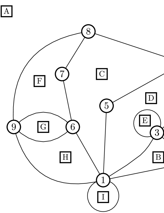
(a) A plane embedding

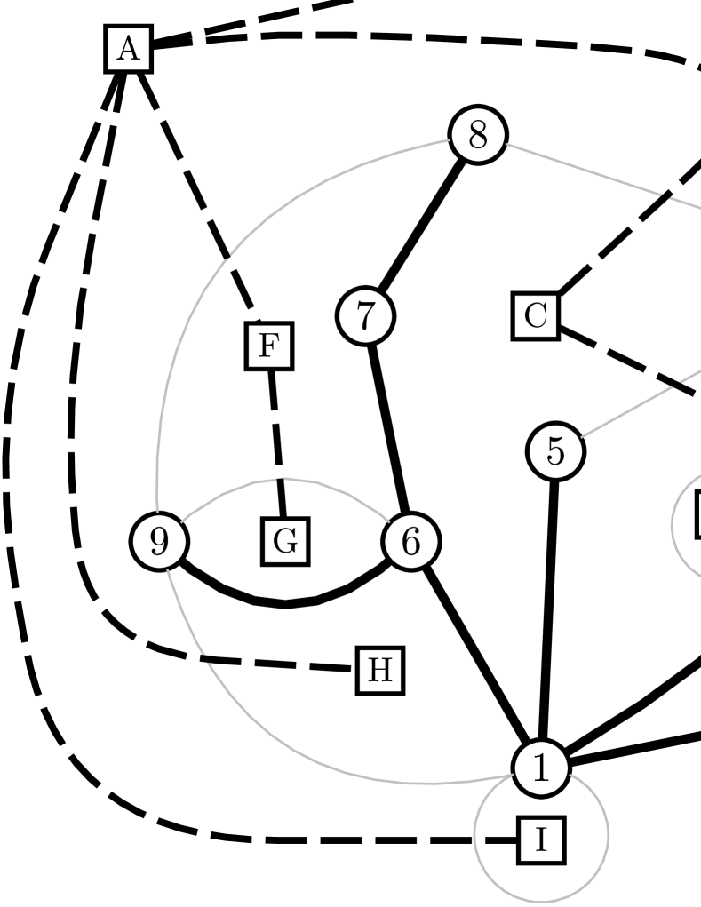
(b) Its primal and dual spanning trees

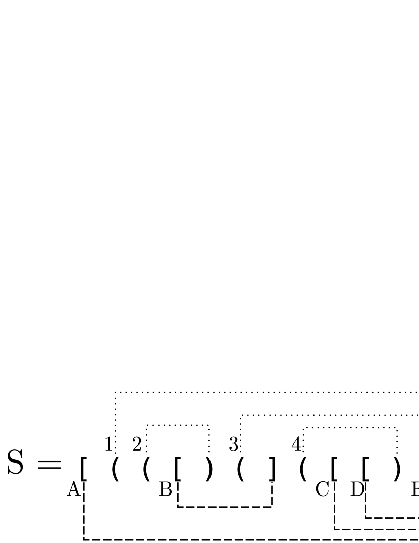
(c) The sequence of parentheses and brackets encoding the plane embedding

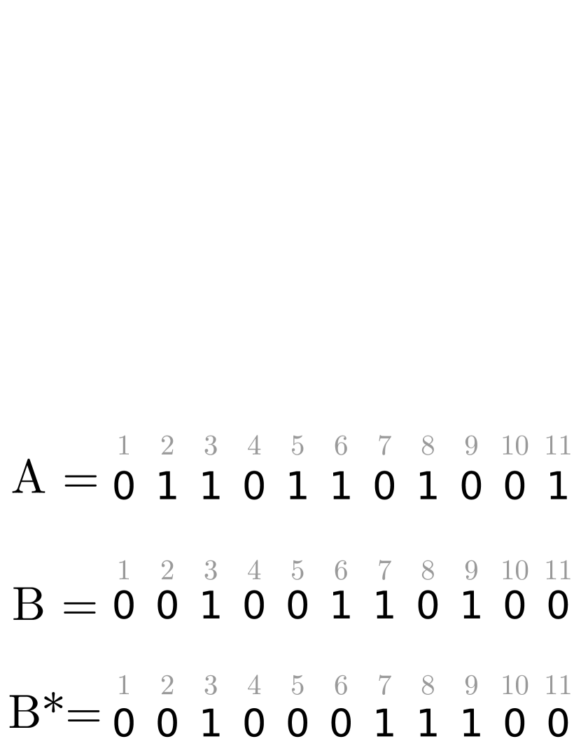
(d) Bitvectors $A$, $B$ and $B^{*}$ representing the sequence $S$

Figure 1: Example of the succinct plane embedding representation of Ferres et al. FFSGHN18 .

Lemma 1 (FFSGHN18 ).

Consider any plane embedding of a planar graph $G$, any spanning tree $T$ of $G$ and the complementary spanning tree $T^{*}$ of the dual $G^{*}$ of $G$. Suppose we perform a depth-first traversal of $T$ starting from any node on the outer face of $G$ and always process the edges incident to the node v we are visiting in counter-clockwise order. At the root, we arbitrarily choose an incidence of the outer face in the root and start from the last edge of the incidence in counterclockwise order; at any other node, we start from the edge immediately after the one to that node’s parent. Then each edge not in $T$ corresponds to the next edge we cross in a depth-first traversal of $T^{*}$.

Here, an incidence of the outer face in the root means a place where the root and the outer face are in contact. For instance, in Fig. 1(b), the traversal can start at edge $(1,1)$, $(1,2)$, or $(1,9)$, taking node $1$ as the spanning tree root.

The compact representation Turan1984 ; FFSGHN18 is based on the traversal of Lemma 1. Starting at the root of any suitable spanning tree $T$, each time we visit for the first time an edge $e$, we write a “(” if $e$ belongs to $T$, or a “[” if not. Each time we visit an edge $e$ for the second time, we write a “)” if $e$ belongs to $T$ or a “]” otherwise. We call $S$ the resulting sequence of $2m$ parentheses and brackets, which are enclosed by an additional pair of parentheses and of brackets that represent the root and the outer face, respectively. Ranks of opening parentheses act as node identifiers, whereas ranks of opening brackets act as face identifiers. Further, positions in $S$ act as edge identifiers: each edge is identified twice, first by an opening parenthesis or bracket, and later by its corresponding closing parenthesis or bracket.

Fig. 1(c) shows the sequence $S$ for the plane embedding of Fig. 1(b), starting the traversal at the edge $(1,2)$. Observe that the parentheses of $S$ encode the balanced-parentheses representation of $T$ and the brackets encode the balanced-parentheses representation of the dual spanning tree $T^{*}$. In general the representation of a node $v$, $(\cdots)$ where “(” is the $v$th opening parenthesis, contains the sequences of nested parenthesis sequences for the children of $v$ in $T$ (e.g., the sequence for node $1$ in the figure contains those of the nodes $2$ and $8$), interspersed with top-level brackets (i.e., brackets not contained in the sequence of a child of $v$). Those brackets represent the other edges incident on $v$ (e.g., the “]” of G and the “[ ]” of H). Since the brackets also represent the faces of $G$, if we exchange the roles of brackets and parentheses, the sequence represents the dual graph $G^{*}$.

In the succinct representation of Ferres et al. FFSGHN18 , the sequence $S$ is stored in three bitvectors, $A[1..2(m+2)]$, $B[1..2n]$, and $B^{*}[1..2(m-n+2)]$. It holds that $A[i]=1$ if the $i$th entry of $S$ is a parenthesis, and $A[i]=0$ if it is a bracket. Bitvector $B$ stores the balanced sequence of parentheses of $S$, storing a $0$ for each opening parenthesis and a $1$ for each closing parenthesis. Bitvector $B^{*}$ stores the balanced sequence of brackets of $S$ in a similar way. Fig. 1(d) shows the bitvectors that store the sequence $S$ of Fig. 1(c).

Adding support for $rank$ and $select$ operations on $A$, $B$ and $B^{*}$, and for $open$, $close$ and $enclose$ (i.e., $parent$) operations on $B$ and $B^{*}$, we simulate their support on $S$, as follows ($match(S,i)$ and $enclose(S,i)$ give the parenthesis or bracket matching or enclosing, respectively, the one at $S[i]$):

$$\small S[i]=\left\{\begin{array}[]{ll}\mbox{``{\tt(}''}&\textrm{if }A[i]=1\land B[rank_{1}(A,i)]=0,\\ \mbox{``{\tt)}''}&\textrm{if }A[i]=1\land B[rank_{1}(A,i)]=1\\ \mbox{``{\tt[}''}&\textrm{if }A[i]=0\land B^{*}[rank_{0}(A,i)]=0,\\ \mbox{``{\tt]}''}&\textrm{if }A[i]=0\land B^{*}[rank_{0}(A,i)]=1\\ \end{array}\right.$$

$$\small rank_{c}(S,i)=\left\{\begin{array}[]{ll}rank_{0}(B,rank_{1}(A,i))&\textrm{if~{}}c=\mbox{``{\tt(}''},\\ rank_{1}(B,rank_{1}(A,i))&\textrm{if~{}}c=\mbox{``{\tt)}''}\\ rank_{0}(B^{*},rank_{0}(A,i))&\textrm{if~{}}c=\mbox{``{\tt[}''},\\ rank_{1}(B^{*},rank_{0}(A,i))&\textrm{if~{}}c=\mbox{``{\tt]}''}\\ \end{array}\right.$$

$$\small select_{c}(S,i)=\left\{\begin{array}[]{ll}select_{1}(A,select_{0}(B,i))&\textrm{if~{}}c=\mbox{``{\tt(}''},\\ select_{1}(A,select_{1}(B,i))&\textrm{if~{}}c=\mbox{``{\tt)}''}\\ select_{0}(A,select_{0}(B^{*},i))&\textrm{if~{}}c=\mbox{``{\tt[}''},\\ select_{0}(A,select_{1}(B^{*},i))&\textrm{if~{}}c=\mbox{``{\tt]}''}\\ \end{array}\right.$$

$$\small match(S,i)=\left\{\begin{array}[]{llll}select_{1}(close(B,rank_{1}(A,i)))&\textrm{if~{}}S[i]=\mbox{``{\tt(}''},\\ select_{1}(open(B,rank_{1}(A,i)))&\textrm{if~{}}S[i]=\mbox{``{\tt)}''},\\ select_{0}(close(B^{*},rank_{0}(A,i)))&\textrm{if~{}}S[i]=\mbox{``{\tt[}''},\\ select_{0}(open(B^{*},rank_{0}(A,i)))&\textrm{if~{}}S[i]=\mbox{``{\tt]}''}\\ \end{array}\right.$$

$$\small enclose(S,i)=\left\{\begin{array}[]{ll}select_{1}(enclose(B,rank_{1}(A,i)))&\textrm{if }S[i]=\mbox{``{\tt(}''}\\ select_{0}(enclose(B^{*},rank_{0}(A,i)))&\textrm{if }S[i]=\mbox{``{\tt[}''}\\ \end{array}\right.$$

With those primitives, the succinct representation of Ferres et al. FFSGHN18 supports constant-time operations to navigate the embedding. Precisely, the representation supports the following operations:

$first(v)/last(v)$:

the position in $S$ of the first/last visited edge of the node $v$;

$mate(i)$:

the position in $S$ of the other occurrence of the $i$th visited edge;

$next(i)/prev(i)$:

the position of the next/previous edge after visiting the $i$th edge of a node $v$ in counter-clockwise order; and

$node(i)$:

the index of the node we are visiting when the traversal reaches the $i$th edge.

The index $v$ of the nodes corresponds to their order in the depth-first traversal of the spanning tree $T$, whereas the index $i$ of a visited edge is just a position in $S$ (since each edge is visited twice, it has two positions in $S$, and $node(\cdot)$ is different on them). The operations are then supported as follows FFSGHN18 :

• By Lemma 1, the first visited edge of a node $v$ is immediately after the edge to the parent of $v$ in $T$ (except for the root of $T$), thus $first(v)=select_{\mbox{``{\tt(}''}}(S,v)+1$. The last visited edge of $v$ is the one returning to its parent, $last(v)=match(S,select_{\mbox{``{\tt(}''}}(S,v))$.

• The operation $mate(i)$ is just $match(S,i)$.

• The implementation of $next(i)$ depends on whether the $i$th visited edge belongs to $T$ or not. Specifically, $next(i)=i+1$ unless $S[i]=\mbox{``{\tt(}''}$, in which case it is instead $next(i)=match(S,i)+1$. Analogously, $prev(i)=i-1$ unless $S[i-1]=\mbox{``{\tt)}''}$, in which case it is $match(S,i-1)$.

• Operation $node(i)$ also depends on whether $S[i]$ is a parenthesis or a bracket. In the first case, the edge is in $T$ and connects $i$ with its parent. The source is the parent, $rank_{\mbox{``{\tt(}''}}(S,enclose(S,i))$, if $S[i]=\mbox{``{\tt(}''}$, or the mate of $i$, $rank_{\mbox{``{\tt(}''}}(S,match(S,i))$, if $S[i]=\mbox{``{\tt)}''}$. On brackets (i.e., $S[i]=\mbox{``{\tt[}''}$ or “]”), we must find the lowest node of $T$ containing the bracket. That is, letting $j=select_{1}(A,rank_{1}(A,i))$ be the position of the last parenthesis preceding $i$, $node(i)=rank_{\mbox{``{\tt(}''}}(S,j)$ if $S[j]=\mbox{``{\tt(}''}$, and $node(i)=rank_{\mbox{``{\tt(}''}}(S,enclose(S,match(S,j)))$ otherwise.

With the operations described above, we can implement more complex queries in optimal time, such as listing all the incident edges of a node $v$ in constant time per returned element, and listing all the edges or nodes bordering a face given an edge of the face, spending constant time per returned element. Other operations, such as the degree of a node and checking if two nodes are neighbors, are not supported in constant time. For the degree of a node $v$, the representation supports any time in $\omega(1)$, whereas for the adjacency test of two nodes $u$ and $v$, they achieve any time in $\omega(\log m)$. Theorem 2 summarizes the results of Ferres et al.

Theorem 2 (FFSGHN18 ).

An embedding of a connected planar graph with $m$ edges can be represented in $4m+o(m)$ bits, supporting the listing in clockwise or counter-clockwise order of the neighbors of a node and the nodes bordering a face in $O(1)$ time per returned node. One can also find the degree of a node in any time in $\omega(1)$, and check if two nodes are adjacent in any time in $\omega(\log m)$.

4 Some Simple Results

As a warm-up exercise, we start with some results that derive easily from previous work FFSGHN18 , but that have not been clearly stated.

4.1 Nodes and Faces Connected by an Edge

We first obtain the nodes connected by a given edge, and its dual, the faces separated by the edge. This trivially answers queries (1.a) and its dual (1.b), (2.a) and its dual (2.b), (3.a) and its dual (3.b), all in constant time.

Note that our edge representation, as positions in $S$, is valid for both $G$ and its dual $G^{*}$: by Lemma 1, the spanning tree edges of $G$, marked with parentheses in $S$, are exactly the non-spanning tree edges of $G^{*}$, and vice versa, the brackets in $S$ are the spanning-tree edges of $G^{*}$ and the non-spanning tree edges of $G$. We then define a new operation, $face(i)$, that returns the identifier of the face where the traversal of $G^{*}$ is when we traverse edge $i$. This is solved analogously to $node(i)$, by exchanging the meaning of parentheses and brackets:

• If $S[i]$ is a bracket, then $face(i)=rank_{\mbox{``{\tt[}''}}(S,enclose(S,i))$ if $S[i]=\mbox{``{\tt[}''}$, and $face(i)=rank_{\mbox{``{\tt[}''}}(S,match(S,i))$ if $S[i]=\mbox{``{\tt]}''}$. If $S[i]$ is a parenthesis, we compute the position $j=select_{0}(A,rank_{0}(A,i))$ of the last bracket preceding $i$; then $face(i)=rank_{\mbox{``{\tt[}''}}(S,j)$ if $S[j]=\mbox{``{\tt[}''}$, and $face(i)=rank_{\mbox{``{\tt[}''}}(S,enclose(S,match(S,j)))$ otherwise.

The result is trivial once we can compute operations $node(\cdot)$ and $face(\cdot)$.

Lemma 2.

The representation of Theorem 2 can determine in $O(1)$ time the two nodes connected by an edge, and the two faces separated by an edge.

Proof: The two nodes corresponding to an edge $i$ in $G$ are simply $node(i)$ and $node(match(S,i))$. The two faces are $face(i)$ and $face(match(S,i))$.

4.2 Listing Queries

Listing the faces bordering a given face (3.d) can be done as the dual of listing the neighbors of a node (3.c), by exchanging the roles of brackets and parentheses in Theorem 2. Listing the faces incident on a node (3.e) can also be done as a subproduct of Theorem 2. For each edge $e$ incident on $u$, obtained in counter-clockwise order, we obtain the faces $e$ divides using Lemma 2. This lists all the faces incident on $u$, in counter-clockwise order, with the only particularity that each face is listed twice, consecutively. Analogously, given a face identifier $x$, we can list the nodes found in the frontier of the face (3.f). This query is not exactly the same as in Theorem 2, because there we must start from an edge bordering the desired face.

Lemma 3.

The representation of Theorem 2 suffices to list, given a node $u$, the faces incident on $u$ in counter-clockwise order from its parent in $T$, each in $O(1)$ time, or given a face $x$, the nodes in the frontier of $x$ in clockwise order from its parent in $T^{*}$, each in $O(1)$ time.

4.3 Counting Queries

Ferres et al. FFSGHN18 count the number of edges incident on a node $u$ (4.a) in $O(f(m))$ time using $o(m)$ bits, for any $f(m)\in\omega(1)$. A bitvector of length $O(m)$ with $O(m/f(m))$ 1s marks the nodes with degree $f(m)$ or more; this bitvector requires $O(m\log f(m)/f(m))+o(m)$ bits in compressed form RRR07 . For nodes with degree below $f(m)$, they traverse the neighbors one by one; for the others, they store the degree explicitly in another bitvector using $O(m\log f(m)/f(m))\subseteq o(m)$ further bits.

We can similarly count the number of neighboring nodes or faces, with the exception that we can reach several times the same node or face as we traverse the edges incident on a node. Thus, we need time $O(f(m)\log f(m))$ on nodes with degree over $f(m)$ in order to remove repetitions; for higher-degree nodes we store the correct number explicitly. We then obtain $O(f(m)\log f(m))$ time using $o(m)$ bits, which still achieves any time in $\omega(1)$. By building the structure on the dual of $G$, we count the number of edges, nodes, or faces in the frontier of a face $x$ (4.b).

5 Deciding if Two Nodes/Faces Share an Edge

Ferres et al. FFSGHN18 show how we can determine if two given nodes $u$ and $v$ are connected in any time $f(m)\in\omega(\log m)$. First, they check in constant time if they are connected by an edge of the spanning tree $T$: one must be the parent of the other. Otherwise, the nodes can be connected by an edge not in $T$, represented by a pair of brackets. Their idea is to mark in a bitvector $D[1..n]$ the nodes having $f(m)$ neighbors or more (see Fig.2(d) for an example). The subgraph $G^{\prime}$ induced by the marked nodes, where they also eliminate self-loops and multi-edges, has $n^{\prime}\leq 2m/f(m)$ nodes, because at least $f(m)$ edges are incident on each marked node and each of the $m$ edges are incident on $2$ nodes. Since $G^{\prime}$ is planar and simple, it can have only $m^{\prime}<3n^{\prime}\leq 6m/f(m)$ edges. They represent $G^{\prime}$ using adjacency lists, which use $o(m)$ bits as long as $f(m)\in\omega(\log m)$. Given two nodes $u$ and $v$, if either of them is not marked in $D$, they simply enumerate its neighbors in time $O(f(m))$ to check for the other node. Otherwise, they map both to $G^{\prime}$ using $rank_{1}(D)$, and binary search the adjacency list of one of the nodes for the presence of the other, in time $O(\log m)\subseteq o(f(m))$. Bitvector $D$ has $n^{\prime}\leq 2m/f(m)$ bits set out of $n\leq m+1$ (this second inequality holds because $G$ is connected), and therefore it can be represented using $(2m/f(m))\log(f(m)/2))+O(m/f(m))+o(m)\subseteq o(m)$ bits while answering $rank$ queries in constant time RRR07 .

We will obtain any time $f(m)\in\omega(1)$ by solving the query on $G^{\prime}$ in a different way. This requires a more complex mapping, however, because now we cannot afford to represent the node identifiers of $G^{\prime}$ in explicit form within $o(m)$ bits.

In particular, we will not physically remove (all) the unmarked nodes of $G$ to form $G^{\prime}$; we just paint the unmarked nodes to signal that they can be removed. We do, instead, remove useless edges not in the spanning tree $T$. More precisely, we start with $G^{\prime}=G$ and then:

• Paint the low-degree nodes $u$ in gray; say the high-degree ones are black.

• Remove the edges incident on gray nodes $u$ and not belonging to $T$.

• Remove self-loops and multiple edges, though never choosing an edge of $T$.

The spanning tree $T^{\prime}$ of $G^{\prime}$ is in principle identical to $T$. Note that the only remaining neighbors of gray nodes are connected by edges in $T^{\prime}$. In order to obtain the desired space/time performance the gray nodes must be reduced, yet without affecting the traversal order of $T^{\prime}$ on the remaining nodes. We thus perform the following additional pruning on $G^{\prime}$ and $T^{\prime}$:

1. Consecutive gray siblings in $T^{\prime}$, if their parent has no other edges between them in $G^{\prime}$, are merged into one, and their children list are concatenated.

2. A gray node with only one child that is also gray is removed, and its child is connected to its parent.

3. Gray nodes that are leaves in $T^{\prime}$ are removed.

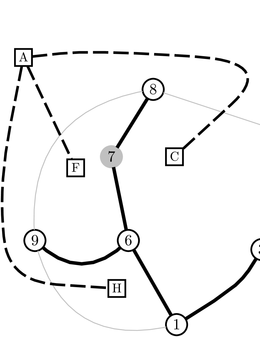
(a) Graph $G^{\prime}$ with $f(m)=3$

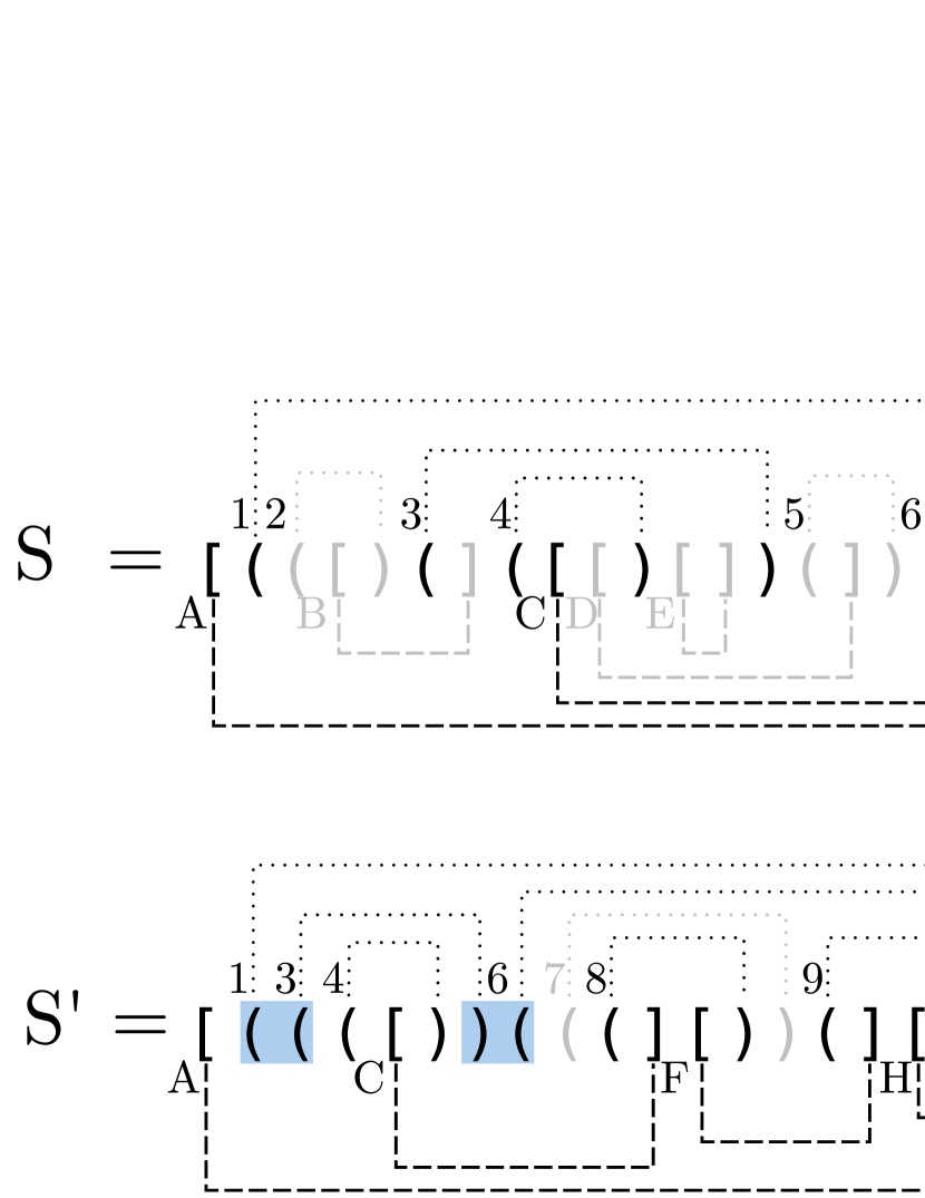
(b) Parentheses/brackets representation of $G^{\prime}$

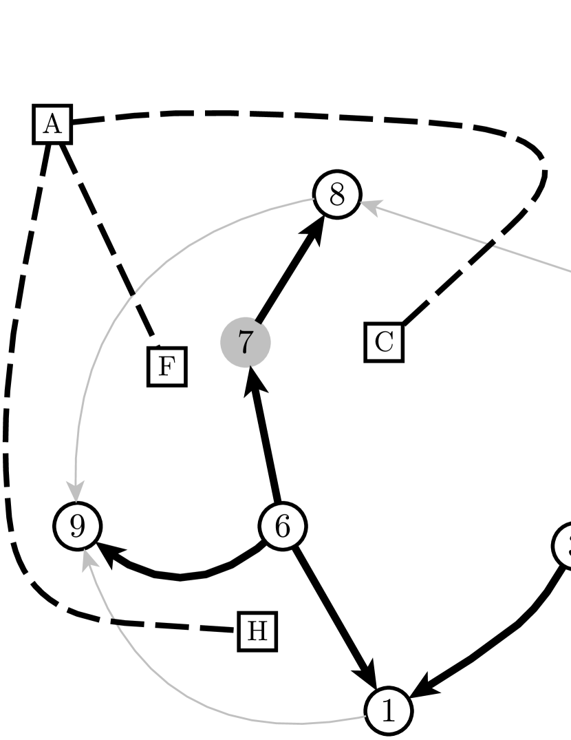
(c) Oriented graph $G^{\prime}$

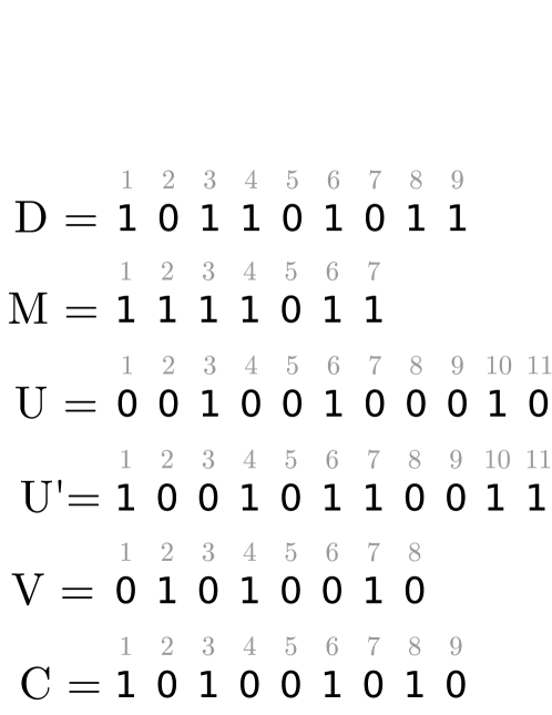
(d) Bitvectors $D$, $M$, $U$, $U^{\prime}$, $V$ and $C$

Figure 2: Graph $G^{\prime}$ used to support query (1.c). (2(a)) Graph $G^{\prime}$ after applying all the pruning rules, with $f(m)=3$; node $7$ is the only gray node that remains. (2(b)) The representation of $G^{\prime}$. On the top we mark the gray nodes and removed edges in $S$. On the bottom we show the final sequence $S^{\prime}$; we also highlight in blue the range of parentheses and brackets representing the children of node 1. (2(c)) Graph $G^{\prime}$ with oriented edges. (2(d)) Bitvectors $D$, $M$, $U$, $U^{\prime}$, $V$, and $C$ used to support query (1.c).

Fig. 2(a) shows the graph $G^{\prime}$ for the graph $G$ of Fig. 1(a), with $f(m)=3$.

As seen, $G^{\prime}$ has $n^{\prime}\leq 2m/f(m)$ black nodes. It has also gray nodes, but by rules (1–3) above, every gray node has a first or a second child in $T^{\prime}$ that is black (recall that all the edges of a gray node are in $T^{\prime}$, so rule (1) leaves no consecutive gray children of a gray node in $T^{\prime}$). Thus, $G^{\prime}$ has at most $n^{\prime}$ gray nodes. Further, since $G^{\prime}$ is simple and contains at most $2n^{\prime}$ nodes (black or gray), it contains $m^{\prime}<6n^{\prime}$ edges. The length of the sequence $S^{\prime}$ representing $G^{\prime}$ is then $2m^{\prime}+4<12n^{\prime}+4\leq 24m/f(m)+4\in O(m/f(m))\subseteq o(m)$.

We use an additional bitvector $M$ that identifies with 1s the black nodes of $T^{\prime}$, in preorder. Therefore, to map the identifier $u$ of a marked node in $G$ (i.e., $D[u]=1$), we first compute $u^{\prime\prime}=rank_{1}(D,u)$, which is its preorder position among the black nodes of $T^{\prime}$. We then compute $u^{\prime}=select_{1}(M,u^{\prime\prime})$ to obtain its node identifier in $T^{\prime}$. Its opening parenthesis in $S^{\prime}$ is then at $select_{\mbox{``{\tt(}''}}(S^{\prime},u^{\prime})$. The length of $M$ is at most $2n^{\prime}\in o(m)$. An example of the bitvector $M$ can be seen Fig. 2(d).

The key idea to determine if (black) nodes $u^{\prime}$ and $v^{\prime}$ are connected in $G^{\prime}$ is that one can orient the edges in a simple planar graph so that every node has outdegree at most $3$ CE91 . Once $G^{\prime}$ is oriented, determining whether $(u^{\prime},v^{\prime})$ is an edge of $G^{\prime}$ requires testing whether at most $6$ edges connect $u^{\prime}$ and $v^{\prime}$ (i.e., the $3$ edges leaving $u^{\prime}$ and the $3$ edges leaving $v^{\prime}$). For instance, Fig. 2(c) shows a possible orientation for the edges of graph $G^{\prime}$ of Fig. 2(a).

The problem then reduces to finding each of the out-edges of a node $u^{\prime}$ fast. We can focus on the edges not in $T^{\prime}$, because we always start checking whether $(u,v)$ or $(v,u)$ are in $T$, and the edges between black nodes of $T^{\prime}$ also belong to $T$. We will find in constant time the (at most) $3$ brackets that represent out-edges in the top level of the sequence $(\cdots)$ that describes $u^{\prime}$ (we say that those brackets are marked). Recall that this sequence contains the sub-sequences $(\cdots)$ of the children $u_{1},\ldots,u_{k}$ of $u^{\prime}$ in $T^{\prime}$, interspersed with brackets.

We proceed as follows. We define a bitvector $U$ where we traverse $T^{\prime}$ in preorder and, for each black node $u^{\prime}$ with $k$ children $u_{1},\ldots,u_{k}$, we add $k+1$ bits. The first bit is $1$ iff there are marked brackets between the opening parenthesis of $u^{\prime}$ and the opening parenthesis of $u_{1}$ (or, if $u^{\prime}$ has no children, between the opening and closing parentheses of $u^{\prime}$). For $1<j\leq k$, the $j$th of the $k+1$ bits is $1$ iff there are marked brackets between the closing parenthesis of $u_{j-1}$ and the opening parenthesis of $u_{j}$. Finally, the $(k+1)$th bit is a $1$ iff there are marked brackets between the closing parenthesis of $u_{k}$ and that of $u^{\prime}$. Since $T^{\prime}$ has at most $2n^{\prime}$ nodes and at most $2n^{\prime}-1$ of those are children of some node, the length of $U$ is $<4n^{\prime}\in O(m^{\prime})$. A second bitvector, $U^{\prime}$, marks with $1$s the first of the $k+1$ bits of each node described in $U$. Finally, we use a third bitvector $V$ of length $O(m^{\prime})$, where $V[i]=1$ means that the $i$th bracket, left to right in $S^{\prime}$, is marked. For example, the bitvectors $U$, $U^{\prime}$ and $V$ for the graph of Fig. 2(c) are shown in Fig. 2(d).

To find the out-neighbors of a node $u^{\prime}$, we first find its area $U[p..p^{\prime}]$, with $p=select_{1}(U^{\prime},u^{\prime})$ and $p^{\prime}=select_{1}(U^{\prime},u^{\prime}+1)-1$. We now find the (up to $3$) positions $p_{i}\in[p..p^{\prime}]$ where $U[p_{i}]=1$, with $p_{i}=select_{1}(U,rank_{1}(U,p-1)+i)$, stopping when $p_{i}>p^{\prime}$. For each of those $p_{i}$, we must search the area of brackets that lie between the $(p_{i}-p)$th and the $(p_{i}-p+1)$th children of $u^{\prime}$. Let $u^{\prime}$ have $k$ children. The area between the $0$th and the $1$st children refers to $S^{\prime}[select_{\mbox{``{\tt(}''}}(S^{\prime},u^{\prime})+1..select_{\mbox{``{\tt(}''}}(S^{\prime},u^{\prime}+1)-1]$. The area between the $i$th and the $(i+1)$th children, for $1\leq i\leq k$, refers to $S^{\prime}[match(S^{\prime},child(S^{\prime},u^{\prime},i))+1..child(S^{\prime},u^{\prime},i+1)]$, where we extend the operation $child$ to operate on the parentheses of the sequence $S^{\prime}$ as follows:

$$child(S^{\prime},u^{\prime},i)=select_{1}(A^{\prime},child(B^{\prime},select_{0}(B^{\prime},u^{\prime}),i)),$$

where we assume $S^{\prime}$ is represented with bitvectors $A^{\prime}$, $B^{\prime}$, and $(B^{*})^{\prime}$. Finally, the area between the $k$th and the $(k+1)$th children of $u^{\prime}$ refers to $S^{\prime}[match(S^{\prime},child(S^{\prime},u^{\prime},k))+1..match(S^{\prime},u^{\prime})-1]$.

Let $S^{\prime}[q..q^{\prime}]$ be any such area of $S^{\prime}$, which is composed of only brackets. We map $q$ and $q^{\prime}$ to $V$ with $r=rank_{0}(A^{\prime},q)$ and $r^{\prime}=r+(q^{\prime}-q)$, so we must enumerate the (up to 3) 1s in $V[r..r^{\prime}]$. Those are $r_{i}=select_{1}(V,rank_{1}(V,r-1)+i)$, stopping when $r_{i}>r^{\prime}$. The corresponding marked brackets are $q_{i}=r_{i}+(q-r)$. Each position $S^{\prime}[q_{i}]$ corresponds to an edge that must be tested to see if it is incident on $v^{\prime}$, in constant time with query (2.a). We then analogously check if the up to $3$ out-neighbors of $v^{\prime}$ are incident on $u^{\prime}$.

If we further wish to retrieve the positions $S[b..b^{\prime}]$ of a pair of brackets that connect $u^{\prime}$ and $v^{\prime}$, when the edge does not trivially belong to $T$, we enrich our structure with bitvector $C$, which tells which face identifiers of $G$ (i.e., ranks of opening brackets) survive in $G^{\prime}$. See the bottom of Fig. 2(d) for an example. Once we find that $u^{\prime}$ and $v^{\prime}$ are neighbors connected by the edge $S^{\prime}[x..x^{\prime}]=[\cdots]$, we have that the opening bracket number $b^{\prime}=rank_{\mbox{``{\tt[}''}}(S^{\prime},x)$ connects them in $G^{\prime}$. We then identify the edge in $G$ with $b=select_{1}(C,b^{\prime})$, and $mate(b)$, in $O(1)$ additional time. The length of bitvector $C$ is less than $m$ and it has less than $m^{\prime}$ 1s, thus it can be represented in $O(m\log f(m)/f(m))+o(m)\subseteq o(m)$ bits RRR07 .

We thus solve query (1.c) with $o(m)$ extra bits of space and $O(f(m))$ time, for any $f(m)\in\omega(1)$.

Lemma 4.

The representation of Theorem 2 can be enriched with $o(m)$ bits so that we can determine whether two nodes are connected in any time in $\omega(1)$.

5.1 Determining Adjacency of Faces

By exchanging the interpretation of parentheses and brackets, the same sequence $S$ represents the dual $G^{*}$ of $G$, where the roles of nodes and faces are exchanged. We can then use the same solution of Lemma 4 to determine whether two faces are adjacent (1.d). We do not explicitly store the sequence $S^{*}$ representing $G^{*}$, since we can simulate it using $S$. We do, instead, build a structure on $S^{*}$ analogous to the one we built on $S$, creating sequence $(S^{*})^{\prime}$ and its auxiliary bitvectors. This time, the input to the query are the ranks of the opening brackets representing both faces (i.e., node identifiers in $G^{*}$). We then solve query (1.d).

Lemma 5.

The representation of Theorem 2 can be enriched with $o(m)$ bits so that we can determine whether two faces are adjacent in any time in $\omega(1)$.

6 Determining Incidence of a Face in a Node

Given a node $u$ and a face $x$, the problem is to determine whether $x$ is incident on $u$ (2.c). Since with Lemma 3 we can list each face incident on $u$ in constant time, or each node bordering $x$ in constant time, we can use a scheme combining those of Lemmas 4 and 5: If $u$ has less than $f(m)$ neighbors, we traverse them looking for $x$. Otherwise, if $x$ has less than $f(m)$ bordering nodes, we traverse them looking for $u$. We now show how to handle the remaining case.

We define a graph $G^{\#}$ where we add additional nodes representing selected faces of $G$, that is, those having at least $f(m)$ nodes in their frontier. The queries that are not handled by enumeration in $G$ will become a node neighbor query on $G^{\#}$, and solved as in Lemma 4. The graph $G^{\#}$, which will have $O(m)$ edges, will not be represented directly.

Concretely, $G^{\#}$ adds to $G$ a new node $v(x)$ per selected face $x$, as well as new edges connecting $v(x)$ with all nodes in the frontier of $x$. Note $G^{\#}$ is planar because we can draw $v(x)$ inside the face $x$. There are at most $2m/f(m)$ selected faces $x$, because each has at least $f(m)$ edges in its frontier and each edge is in the frontier of two faces. The graph $G^{\#}$ contains $n^{\prime}\leq n+2m/f(m)=O(m)$ nodes and $m^{\prime}\leq 3m$ edges (each selected face limited by $j$ edges of $G$ adds $j$ new edges in $G^{\#}$, and each edge of $G$ limits two faces).

A spanning tree $T^{\#}$ for $G^{\#}$ is built by extending the spanning tree $T$ of $G$ with leaves $v(x)$, as follows. Consider the traversal of $G$ that defines the spanning trees $T$ and $T^{*}$. Let $(u,v)\not\in T$ be the edge in the frontier of a selected face $x$ where the traversal of $T^{*}$ first reaches the face $x$, that is, when edge $(y,x)$ is added to $T^{*}$ for some face $y$. Right after visiting the edge $(u,v)$, we add a new leaf node $v(x)$, as a child of $u$, to $T^{\#}$. We also add the edges $(x,w)$ for the other nodes $w$ in the frontier of face $x$; those edges will not belong to $T^{\#}$. An example of $G^{\#}$ and $T^{\#}$ is shown in Fig. 3(a).

To generate the sequence $S^{\#}$ representing $G^{\#}$ we traverse $T^{\#}$ starting from the edge that connects the outer face with the starting node that generates the sequence $S$. After that, the traversal follows the same order of $T$. When we reach an original selected face $x$ (which in $G^{\#}$ is partitioned into $j$ triangles), we will visit the edge $(u,v(x))\in T^{\#}$ right after $(u,v)\not\in T^{\#}$. We will then traverse the other $j-1$ edges incident on $v(x)$, none of which is in $T^{\#}$, and all of which are visited for the first time because we had not entered face $x$ before. Therefore, the “[” that represents $(u,v)$ in $S^{\#}$ will be immediately followed by $(~{}[^{j-1})$, and then the normal layout of $T$ will follow. Those opening brackets will be closed later along the traversal. Fig. 3(b) shows the sequence $S^{\#}$ obtained after traversing the spanning tree $T^{\#}$ of Fig. 3(a), starting from the edge $(1,A)$. For instance, face $C$ is bounded by the nodes 1, 5, 4, 8, 7 and 6, which are represented by $(~{}[~{}[~{}[~{}[~{}[~{})$ in Fig. 3(b).

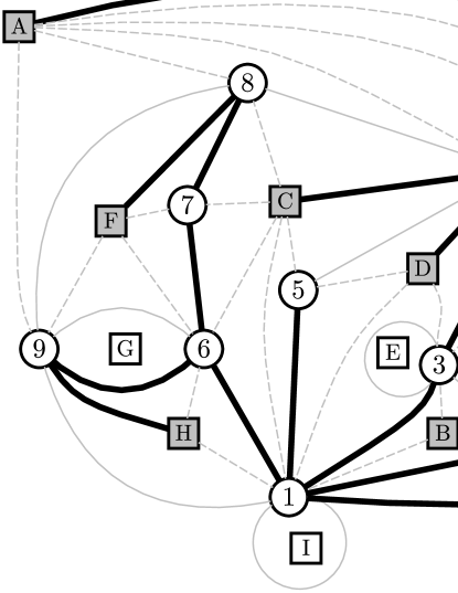
(a) Graph $G^{\#}$ with $f(m)=3$

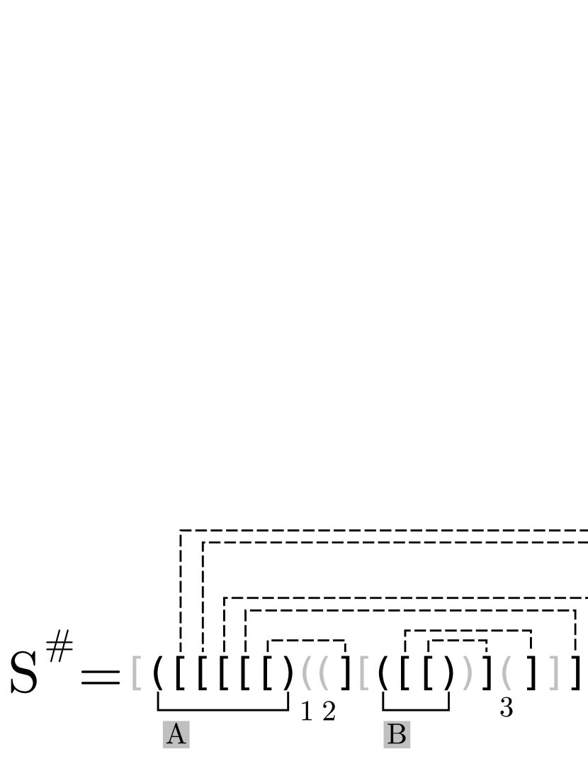
(b) Sequence $S^{\#}$ generated from the graph of Fig. 3(a)

Figure 3: Graph $G^{\#}$ used to support query (2.c). (3(a)) Graph $G^{\#}$ with $f(m)=3$. The selected faces are painted in gray and the spanning tree $T^{\#}$ is represented with thick edges. (3(b)) Sequence $S^{\#}$ obtained from the traversal of $T^{\#}$. The parentheses and brackets added to those in $S$ are in black, so $S$ is the gray subsequence of $S^{\#}$.

This implies that every opening bracket in $S$ representing a selected face $x$, is immediately followed in $S^{\#}$ by an opening parenthesis corresponding to the node $v(x)$ we created for the face. That is, selected faces $x$ in $S$ are in the same order of added nodes $v(x)$ in $S^{\#}$. Further, the nodes of $G$ are in the same order in $S$ and $S^{\#}$. We exploit this correspondence to map nodes and faces from $G$ to nodes of $G^{\#}$ by using the following bitvectors:

• The same bitvector $D[1..n]$ of Section 5, where $D[u]=1$ iff node $u$ of $G$ has at least $f(m)$ neighbors.

• A bitvector $E[1..m-n+1]$, where $E[x]=1$ iff face $x$ of $G$ has at least $f(m)$ nodes (or edges) in its frontier.

• A bitvector $R$ where $R[x^{\prime}]=1$ iff node $x^{\prime}$ of $G^{\#}$ is one of the nodes $v(x)$ we added to $G$ in order to form $G^{\#}$.

If $D[u]=1$, we map it to node $u^{\prime}=select_{0}(R,u)$ in $G^{\#}$ (note that all the nodes in $G$ appear in $G^{\#}$). If $E[x]=1$, we map it to node $x^{\prime}=select_{1}(R,rank_{1}(E,x))$ (only the selected faces in $G$ appear as new nodes in $G^{\#}$). Bitvectors $D$, $E$, and $R$ are of length $O(m)$ and have $O(m/f(m))$ 1s, so they can be represented within $O(m\log f(m)/f(m))+o(m)\subseteq o(m)$ bits RRR07 .

If $u$ has at least $f(m)$ neighbors and $x$ is limited by at least $f(m)$ nodes, we map node $u$ and face $x$ to nodes $u^{\prime}$ and $x^{\prime}$ in $G^{\#}$ as explained, and determine if they are neighbors. Note that, since $x$ has at least $f(m)$ nodes in its frontier, node $x^{\prime}$ has at least $f(m)$ neighbors. Node $u^{\prime}$ also has at least $f(m)$ neighbors in $G^{\#}$, because it had in $G$ and it can only get further neighbors in $G^{\#}$. We then build on $S^{\#}$ the structures of Lemma 4, without explicitly representing $S^{\#}$, so that we can map $u^{\prime}$ and $x^{\prime}$ to the reduced sequence $(S^{\#})^{\prime}$ and solve the query in there. This adds $o(m)$ bits of space and completes the query in any time in $\omega(1)$.

Lemma 6.

The representation of Theorem 2 can be enriched with $o(m)$ bits so that, given a node $u$ and a face $x$, it answers whether $u$ is in the frontier of $x$ in any time in $\omega(1)$.

7 Determining Indirect Connections

To handle queries (5.a) and (5.b), we reuse the idea of selecting a subgraph where the query cannot be solved in time $O(f(m))$ and storing a suitable speed-up structure for those cases. This time, however, the idea leads to a much higher time complexity. We later obtain constant time by relaxing the space requirement to $O(m)$ bits.

Let us first consider determining if two nodes are in the border of the same (unknown) face. Given two nodes $u$ and $v$, if either has less than $f(m)$ neighbors we can traverse its incident faces one by one and, for each face $x$, use Lemma 6 to determine if $x$ is incident on the other node in time $\omega(1)$. For all the pairs of nodes $(u,v)$ where both have $f(m)$ neighbors or more, we store a binary matrix telling whether or not they lie on the same face. This requires $(2m/f(m))^{2}$ bits, which is $o(m)$ for any $f(m)\in\omega(\sqrt{m})$. Thus we can solve query (5.a) and, by duality, query (5.b), in any time in $\omega(\sqrt{m})$.

Lemma 7.

The representation of Theorem 2 can be enriched with $o(m)$ bits so that, given two nodes or two faces, it answers in $O(f(m))$ time whether they share a face or a node, respectively, for any $f(m)\in\omega(\sqrt{m})$.

If we want to know the identity of the shared face (or, respectively, node), this can be stored in the matrix, which now requires $O((m/f(m))^{2}\log m)$ bits. We can then reach any time in $\omega(\sqrt{m\log m})$.

7.1 Constant Times with $O(m)$ Bits of Space

As explained, those operations requiring $\omega(1)$ time in Table 1 automatically become $O(1)$ if we use $f(m)\in O(1)$. In exchange, the space becomes $4+\epsilon$ bits of space for any desired constant $\epsilon>0$. We now show that queries (5.a) and (5.b) can also be solved in $O(1)$ time if we raise the space to $O(m)$ bits. Let us focus on the query of Lemma 7 (5.a); we then obtain (5.b) by duality. Our solution is inspired in a (non-compact) data structure for constant-time bounded shortest distance queries on planar graphs KK06 .

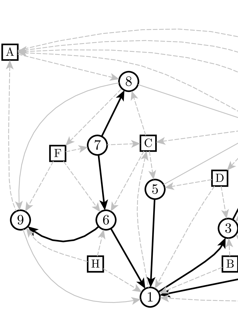
(a) Graph $G^{\#}$ with oriented edges

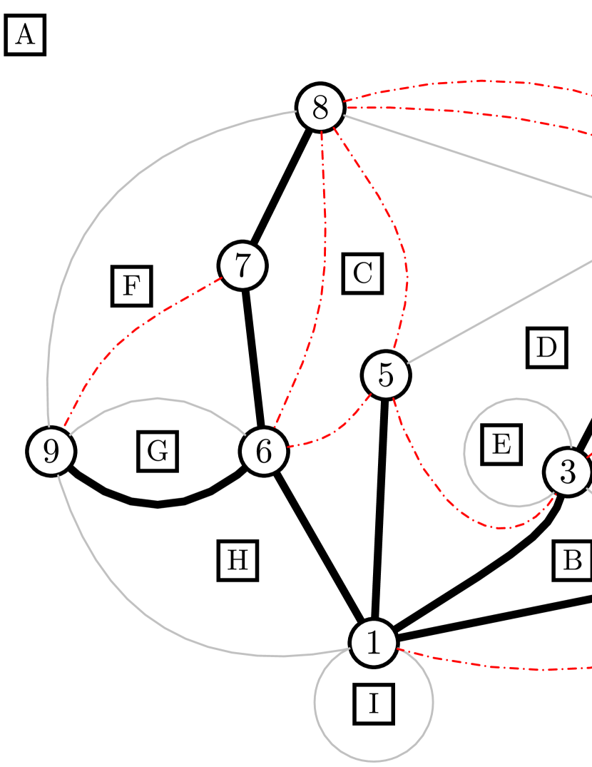
(b) Graph $G^{\$}$

Figure 4: Graphs $G^{\#}$ and $G^{\$}$ used to support query (5.a). (4(a)) Graph $G^{\#}$. Solid edges represent edges of the original graph $G$ (Fig. 1(a)), and dashed ones represent edges connecting faces with their bordering nodes. The spanning tree $T$ of the original graph is in black. (4(b)) Graph $G^{\$}$. Red edges represent the new edges connecting nodes linked by two out-edges of the node induced by their common face in $G^{\#}$.

Consider the graph $G^{\#}$ of Section 6, with the following changes:

• We start with a copy of $G$ and then remove self-loops and multiple edges (not those that belong to $T$). Removing self-loops and multiple edges is irrelevant for the query (5.a).

• We select all the remaining faces of $G$.

• We represent $G^{\#}$ explicitly (so we use $O(m)$ bits of space).

• We orient the edges of $G^{\#}$ as in Section 5. Since $G^{\#}$ is simple, the out-degree of every node can be made at most $3$.

If nodes $u$ and $v$ are both in the frontier of some face mapped to node $x$ in $G^{\#}$, then the following configurations of the edge orientations are possible in $G^{\#}$: $u\rightarrow x\rightarrow v$, $u\rightarrow x\leftarrow v$, $u\leftarrow x\leftarrow v$, and $u\leftarrow x\rightarrow v$. The first three are easily verified in constant time using the structures of Section 6. For example, for $u\rightarrow x\rightarrow v$ we check the (up to) $3$ out-neighbors $x_{i}$ of $u$ and, for those $x_{i}$ that are faces in $G$ (which is verified in bitvector $R$), we check their (up to) $3$ out-neighbors $v_{i,j}$, to see if $v_{i,j}=v$.

The difficult case is $u\leftarrow x\rightarrow v$, because we should start our quest from the unknown node $x$. Fortunately, inside the face $x$ represents in $G$, there can be at most $3$ nodes that are out-neighbors of $x$ in $G^{\#}$. We then create another extended version of the original graph $G$, which we call $G^{\$}$, where we additionally connect those $3$ nodes inside each face $x$, thereby drawing a triangle inside the face (thus $G^{\$}$ is planar). Thus, there is a configuration $u\leftarrow x\rightarrow v$ iff $(u,v)$ is one of those edges of the triangles we have added. Fig. 4(b) shows an example for the graph $G^{\$}$, based on the oriented edges of Fig. 4(a). For instance, the cases $8\leftarrow A\rightarrow 1$ and $5\leftarrow C\rightarrow 6$ cause the insertion of the edges $(1,8)$ and $(5,6)$, as shown in Fig. 4(b). It is clear that $G^{\$}$ has $O(m)$ edges and that we can define a spanning tree $T^{\$}$ for it that is identical to that of $T$, letting all the added edges be not in $T^{\$}$. We then represent $G^{\$}$ as in Lemma 4 (with $f(m)\in O(1)$) and verify the configuration $u\leftarrow x\rightarrow v$ by asking if $u$ and $v$ share an edge in $G^{\$}$. Note that this query can return an edge that belongs to $G$, but in this case it is also true that $u$ and $v$ border the same face. By also considering duality, we have the following result.

Lemma 8.

The representation of Theorem 2 can be enriched with $O(m)$ bits so that, given two nodes or two faces, it answers in $O(1)$ time whether they share a face or a node, respectively.

8 Conclusions

We built on a recent extension FFSGHN18 of Turán’s representation Turan1984 for plane embeddings so as to support a rich set of topological queries within succinct space, $4m+o(m)$ bits for an $m$-edge embedding. Though it exceeds the asymptotically optimal space of $3.58m+o(m)$ bits, this representation is particularly attractive to handle the topological model because it regards the graph and its dual symmetrically, thereby enabling a number of queries relating nodes, edges, and faces.

Starting with an improved solution to determine if two nodes are neighbors, we exploit analogies and duality to support most of the operations in any time in $\omega(1)$. We then relax our space requirements to $O(m)$ bits, showing that in this case we can represent variants of the graph that allow us support all the desired queries (on the original graph) in $O(1)$ time.

An interesting challenge is whether we can support bounded distance queries (bounded meaning that only distances up to some constant $k$ are distinguished) efficiently and within $O(m)$ bits of space. For $k=2$, a relatively obvious variant of Lemma 7 yields any time in $\omega(\sqrt{m})$ within $4m+o(m)$ bits of space. We cannot use an analogous to the $O(m)$-bits construction of Lemma 8 to obtain constant time, however, because the resulting graph $G^{\$}$ could be non-planar. Kowalik and Kurowski KK06 show that this query can be solved in constant time using $O(m\log m)$ bits, that is, with a classical non-compact representation. They use the same idea of orienting the edges and are left with the hard subproblem of the configuration $u\leftarrow x\rightarrow v$, for which we built $G^{\$}$. They handle this case by adding the edges $(u,v)$ explicitly, which in general make the graph non-planar. They show, however, that the resulting graph is the union of a constant number of planar graphs, which can then be queried one by one. Our problem to obtain $O(m)$ bits from this idea is how to track the node identifiers across those planar graphs, which can have very different spanning trees.

References

- \bibcommenthead
- (1) Lozzo, G.D., D’Angelo, A., Frati, F.: On planar greedy drawings of 3-connected planar graphs. Discrete Computational Geometry 63(1), 114–157 (2020)
- (2) Navarro, G.: Compact Data Structures: A Practical Approach. Cambridge University Press, Cambridge, UK (2016)
- (3) Castelli Aleardi, L., Devillers, O., Schaeffer, G.: Succinct representation of triangulations with a boundary. In: Proc. 9th International Conference on Algorithms and Data Structures (WADS), pp. 134–145 (2005)
- (4) Castelli Aleardi, L., Devillers, O., Schaeffer, G.: Succinct representations of planar maps. Theoretical Computer Science 408(2-3), 174–187 (2008)
- (5) Bose, P., Chen, E.Y., He, M., Maheshwari, A., Morin, P.: Succinct geometric indexes supporting point location queries. ACM Transactions on Algorithms 8(2), 10–11026 (2012)
- (6) Turán, G.: On the succinct representation of graphs. Discrete Applied Mathemathics 8(3), 289–294 (1984)
- (7) Ferres, L., Fuentes-Sepúlveda, J., Gagie, T., He, M., Navarro, G.: Fast and compact planar embeddings. Computational Geometry Theory and Applications, 101630 (2020)
- (8) Worboys, M., Duckham, M.: GIS: A Computing Perspective, 2nd edn. CRC Press, Boca Raton, FL, USA (2004)
- (9) Scholl, M.O.: Spatial Databases with Application to GIS. Morgan Kaufmann, San Francisco, CA, USA (2002)
- (10) ISO/IEC 13249-3:2016. Information technology – Database languages – SQL multimedia and application packages – Part 3: Spatial. Technical report (2016)
- (11) Tutte, W.T.: A census of planar maps. Canadian Journal of Mathematics 15, 249–271 (1963)
- (12) Yannakakis, M.: The effect of a connectivity requirement on the complexity of maximum subgraph problems. Journal of the ACM 26, 618–630 (1979)
- (13) Lipton, R.J., Tarjan, R.E.: A separator theorem for planar graphs. SIAM Journal of Applied Mathematics 36, 177–189 (1979)
- (14) Keeler, K., Westbrook, J.: Short encodings of planar graphs and maps. Discrete Applied Mathematics 58, 239–252 (1995)
- (15) He, X., Kao, M.Y., Lu, H.-I.: A fast general methodology for information-theoretically optimal encodings of graphs. SIAM Journal on Computing 30, 838–846 (2000)
- (16) Jacobson, G.: Space-efficient static trees and graphs. In: Proc. 30th Annual Symposium on Foundations of Computer Science (FOCS), pp. 549–554 (1989)
- (17) Munro, J.I., Raman, V.: Succinct representation of balanced parentheses and static trees. SIAM Journal on Computing 31(3), 762–776 (2001)
- (18) Blelloch, G.E., Farzan, A.: Succinct representations of separable graphs. In: Proc. 21st Annual Conference on Combinatorial Pattern Matching (CPM), pp. 138–150 (2010)
- (19) Fuentes-Sepúlveda, J., Navarro, G., Seco, D.: Implementing the topological model succinctly. In: Proc. 26th International Symposium on String Processing and Information Retrieval (SPIRE), pp. 499–512 (2019)
- (20) Clark, D.R.: Compact PAT trees. PhD thesis, University of Waterloo, Canada (1996)
- (21) Raman, R., Raman, V., Satti, S.: Succinct indexable dictionaries with applications to encoding k-ary trees, prefix sums and multisets. ACM Transactions on Algorithms 3(4) (2007)
- (22) Navarro, G., Sadakane, K.: Fully functional static and dynamic succinct trees. ACM Transactions on Algorithms 10(3), 16–11639 (2014)
- (23) Biggs, N.: Spanning trees of dual graphs. Journal of Combinatorial Theory B 11(2), 127–131 (1971)
- (24) Chrobak, M., Eppstein, D.: Planar orientations with low out-degree and compaction of adjacency matrices. Theoretical Computer Science 86(2), 243–266 (1991)
- (25) Cohen, H., Porat, E.: Fast set intersection and two-patterns matching. Theoretical Computer Science 411(40-42), 3795–3800 (2010)
- (26) Patrascu, M., Roditty, L.: Distance oracles beyond the Thorup-Zwick bound. SIAM Journal on Computing 43(1), 300–311 (2014)
- (27) Kowalik, L., Kurowski, M.: Oracles for bounded-length shortest paths in planar graphs. ACM Transactions on Algorithms 2(3), 335–363 (2006)