Planck far-infrared detection of Hyper Suprime-Cam protoclusters at $\bf z\sim 4$: hidden AGN and star formation activity

Abstract

We perform a stacking analysis of Planck, AKARI, Infrared Astronomical Satellite ($IRAS$), Wide-field Infrared Survey Eplorer ($WISE$), and Herschel images of the largest number of (candidate) protoclusters at $z\sim 3.8$ selected from the Hyper Suprime-Cam Subaru Strategic Program (HSC-SSP). Stacking the images of the $179$ candidate protoclusters, the combined infrared (IR) emission of the protocluster galaxies in the observed $12-850~{}\mu$m wavelength range is successfully detected with $>5\sigma$ significance (at $Planck$). This is the first time that the average IR spectral energy distribution (SED) of a protocluster has been constrained at $z\sim 4$. The observed IR SEDs of the protoclusters exhibit significant excess emission in the mid-IR compared to that expected from typical star-forming galaxies (SFGs). They are reproduced well using SED models of intense starburst galaxies with warm/hot dust heated by young stars, or by a population of active galactic nuclei (AGN)/SFG composites. For the pure star-forming model, a total IR (from 8 to 1000 $\mu$m) luminosity of $19.3_{-4.2}^{+0.6}\times 10^{13}~{}L_{\odot}$ and a star formation rate (SFR) of $16.3_{-7.8}^{+1.0}\times 10^{3}~{}M_{\odot}$ yr^-1 are found whereas for the AGN/SFG composite model, $5.1_{-2.5}^{+2.5}\times 10^{13}~{}L_{\odot}$ and $2.1^{+6.3}_{-1.7}\times 10^{3}~{}M_{\odot}$ yr^-1 are found. Uncertainty remaining in the total SFRs; however, the IR luminosities of the most massive protoclusters are likely to continue increasing up to $z\sim 4$. Meanwhile, no significant IR flux excess is observed around optically selected QSOs at similar redshifts, which confirms previous results. Our results suggest that the $z\sim 4$ protoclusters trace dense, intensely star-forming environments that may also host obscured AGNs missed by the selection in the optical.

1 Introduction

Overdense regions at a high redshift known as protoclusters are plausible progenitors of clusters of galaxies today and thus important targets to prove the formation history of galaxy clusters and the giant ellipticals/brightest cluster galaxies (BCGs) therein. Today, many protoclusters are found using the surveys of overdensities of Lyman break galaxies (LBGs; e.g., Steidel et al. 1998; Toshikawa et al. 2012; Ota et al. 2018), Ly$\alpha$ emitters (LAEs; e.g., Kurk et al. 2000; Steidel et al. 2000; Hayashino et al. 2004; Venemans et al. 2007; Kikuta et al. 2019; Higuchi et al. 2019; Harikane et al. 2019), H$\alpha$ emitters (HAEs; e.g., Kurk et al. 2004; Tanaka et al. 2011; Matsuda et al. 2011), and color selection with $Spitzer$ infrared array camera (IRAC) (Galametz et al., 2012; Wylezalek et al., 2013, 2014; Noirot et al., 2016, 2018).

The protoclusters at $z=2-4$, the peak of the cosmic star formation density history (Madau & Dickinson, 2014), are paticularly important targets to constrain the star formation history of cluster galaxies. A bunch of massive galaxies has already appeared in the protoclusters at $z\hskip 3.00003pt\raisebox{1.72218pt}{$<$}\raisebox{-3.01385pt}{$\sim$}\hskip 3.00003pt3$ reported by detecting protocluster galaxies at near-infrared (NIR) such as H$\alpha$ emitters (e.g., Matsuda et al. 2011; Koyama et al. 2013), color selected massive galaxies (e.g., Kodama et al. 2007; Uchimoto et al. 2012; Kubo et al. 2013; Noirot et al. 2016, 2018), including passively evolving galaxies (Kubo et al., 2013; Noirot et al., 2016, 2018; Shimakawa et al., 2018; Shi et al., 2019). During the last decade, overdensities of dusty star-forming galaxies (DSFGs), which have a star formation rate (SFR) of $\sim$ several $100~{}M_{\odot}$ yr^-1 or more but whose ultraviolet (UV) light is absorbed by dust and re-emitted as thermal emission in the infrared (IR) (e.g.,Casey et al. 2014), in protoclusters have been found via deep observations at a mid-IR to mm wavelength using $Spitzer$, $Herschel$ and ground-based sub-milimeter telescopes/arrays (e.g., Tamura et al. 2009; Kato et al. 2016; Wang et al. 2016; Umehata et al. 2017, 2018; Miller et al. 2018; Oteo et al. 2018; Arrigoni Battaia et al. 2018; Gómez-Guijarro et al. 2019; Smith et al. 2019; Harikane et al. 2019). Such DSFGs are likely main progenitors of cluster giant ellipticals because they are compatible with the instantaneous star formation history expected for them. Particularly at the cores of protoclusters, a substantial number of the star formation activities are hidden in the optical but detectable in the IR (e.g., Wang et al. 2016; Umehata et al. 2018; Miller et al. 2018; Oteo et al. 2018). The deep $X$-ray observations show AGN overdensities and an enhanced AGN fraction in protoclusters that indicate the environmental dependence of super massive black hole (SMBH) growth though a wide range of values has been reported (Lehmer et al., 2009; Digby-North et al., 2010; Lehmer et al., 2013; Kubo et al., 2013; Krishnan et al., 2017; Macuga et al., 2019).

Although there is an increasing number of studies of protoclusters, it remains difficult to obtain robust statistics because they are quite rare ($\sim 1.5$ deg^-2 at $z\sim 4$ in Toshikawa et al. 2016). Previous studies have concentrated on high redshift radio galaxies (HzRGs) or luminous QSOs (e.g., Venemans et al. 2007; Matsuda et al. 2011; Kikuta et al. 2019), which are thought to have evolved into the BCGs of today in general while some protoclusters have been found by chance (e.g., Steidel et al. 1998; Spitler et al. 2012; Toshikawa et al. 2012; Ishigaki et al. 2016). The selection bias on them is not clear. In addition, the properties of the known protoclusters vary widely even when they are at the same redshift. Thus there is a strong need for a large statistical study of protoclusters to investigate their typical properties and variations as a function of cluster mass and redshift.

The on-going wide and deep optical imaging survey by the Hyper Suprime-Cam Subaru Strategic Program (HSC-SSP; Aihara et al. 2018) is performing a wide and uniform survey of protoclusters at $z=2-7$ (Toshikawa et al., 2018). At this point, $\approx 180$ protocluster candidates at $z\sim 3.8$ have been found based on the overdensities of LBGs. According to past protocluster studies, the properties of protoclusters observed in the optical are expected to be only “the tip of the iceberg”. However, it is difficult to conduct multi-band follow up observations for such a large catalog of candidates. Particularly, spectral energy distributions (SEDs) in the IR are necessary to constrain the SFR and AGN activities obscured by dust. The Atacama Large Millimeter Array (ALMA) can cover only a portion of the entire IR SEDs. Unfortunately, currently space telescopes capable of detecting the redshifted mid-far IR emission of galaxies at high redshift are not available.

Here we perform the statistical study of the IR properties of the protoclusters by using the archival IR all sky maps. Lately, plausible clusters of DSFGs at $z=2$ to $4$ detected as point sources on Planck high frequency instrument (HFI) sky images has been reported (e.g., Clements et al. 2014, 2016; Greenslade et al. 2018). The spatial resolution and detection limit of the $Planck$ HFI images are too low to discretely identify galaxies at high redshift; however they are useful to evaluate the average total sum flux of protocluster galaxies, though it is difficult to individually detect protoclusters at $z\sim 4$. In this study, the average of all the IR fluxes from a protocluster at $z\sim 3.8$ is shown for the first time, by stacking the publicly available archival IR images taken by Planck (Planck collaboration I, 2011), AKARI (Murakami et al., 2007), Infrared Astronomical Satellite (IRAS: Neugebauer et al. 1984), Wide-Field Infrared Survey Explorer (WISE: Wright et al. 2010), and the Herschel Astrophysical Terahertz Large Area Survey ($H$-ATLAS data release 1, Valiante et al. 2016) of the largest catalog of the candidate protoclusters at $z\sim 3.8$ selected from the HSC-SSP survey.

This paper is organized as follows: in Section 2, the HSC-SSP protocluster catalog and archival IR data are described, in Section 3, the stacking analysis methods are described, in Section 4, the results are presented, and in Section 5, the findings are discussed. Throughout the paper, a $\Lambda$CDM cosmology is adopted with $H_{0}=70$ km s^-1 Mpc^-1, $\Omega_{\Lambda}=0.7$ and $\Omega_{m}=0.3$.

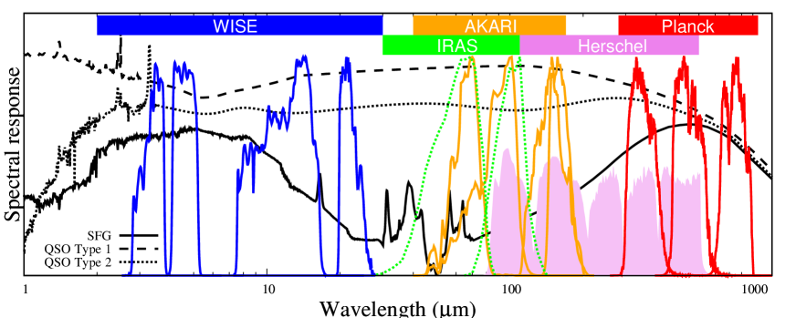
Figure 1: Filter transmission curves for the IR sky surveys used in this study. The red curves at $350-850~{}\mu$m show Planck 353, 545, and 857 GHz. The orange curves at $40-200~{}\mu$m show AKARI N60, WIDE-S, WIDE-L, and N160. The green dotted curves show IRAS 60 and 100 $\mu$m. The violet filled curves show Herschel 100, 160, 250, 350, and 500 $\mu$m. The blue curves at $3-30~{}\mu$m show WISE W1, W2, W3, and W4. The black thick solid, dashed and dotted curves show the SEDs of a SFG, Type-1 QSO and Type-2 QSO from the SED library by Polletta et al. (2006) shifted to $z=3.8$, respectively.

2 Data

2.1 Protocluster catalog

We use the protocluster catalog at $z\sim 3.8$ obtained via a systematic search for high-z protoclusters based on the HSC-SSP survey (Aihara et al., 2018) in Toshikawa et al. (2018). HSC is the prime focus camera with a large field-of-view (FoV) of 1.8 deg² and high sensitivity on Subaru Telescope (Miyazaki et al., 2012). The HSC-SSP survey is an on-going multi-color ($griz$ + narrow band) survey consisting of three layers; the ultradeep (UD; 3.5 deg², $i\sim 28$ mag), deep (26 deg², $i\sim 27$ mag) and wide (1400 deg², $i\sim 26$ mag) layers. Toshikawa et al. (2018) constructed a catalog of LBGs based on the $gri$-band images (hereafter the $g$-dropout galaxies) over an area of 121 deg² of the HSC-SSP wide survey. Their color cut is sensitive to galaxies in the redshift range of $3.3\hskip 3.00003pt\raisebox{1.72218pt}{$<$}\raisebox{-3.01385pt}{$\sim$}\hskip 3.00003ptz\hskip 3.00003pt\raisebox{1.72218pt}{$<$}\raisebox{-3.01385pt}{$\sim$}\hskip 3.00003pt4.2$. Then, they measured the surface density of the $g$-dropout galaxies selected down to a limiting magnitude of $i=25.0$ mag within an aperture of $1.8$ arcmin (0.75 Mpc physical). They then, selected the regions with an overdensity significance of $>4\sigma$ as protocluster candidates. This radius corresponds to the typical extent of the regions that will collapse into a single massive halo with a halo mass $M_{h}>10^{14}~{}M_{\odot}$ by $z=0$ predicted in the cosmological numerical simulations (e.g., Chiang et al. 2013). Because the redshift range of the $g$-dropout galaxies is large, some of the protocluster candidates are probably spurious because of projection effects. They quantified this possible contamination using simulations, finding that at a $4\sigma$ threshold, approximately $>76$ % of the candidate protoclusters are expected to evolve into massive galaxy clusters. According to the correlation function analysis in Toshikawa et al. (2018), the majority of the candidates are expected to evolve into clusters of galaxies with $M_{h}\geq 5\times 10^{14}~{}M_{\odot}$, i.e., the richest clusters today.

They finally selected 216 overdense regions. Of these, 37 are within $8$ arcmin from another overdense region. Because the typical spatial extents of protoclusters drop at $\sim 8$ arcmin (see Fig. 8 of Toshikawa et al. 2016), they can be substructures of larger overdense regions. After merging these regions, they identified 179 unique protocluster candidates. In the following stacking analysis, the archival IR images centered on these 216 density peaks of the $g$-dropout galaxies in each protocluster candidate are cut out.

2.2 IR all sky surveys

We perform a stacking analysis of the protoclusters using the publicly available archival IR images. We use Planck, AKARI, IRAS, and WISE all sky survey, and $H$-ATLAS. Fig. 1 shows their filter transmission curves. They cover a large portion of the IR SEDs of galaxies at $z\sim 4$. Table 6 in the Appendix summarizes the central wavelengths, full width at half-maximum (FWHM) of the point spread functions (PSFs), point source detection limits, and expected sky noises on the stacked images. In the following, we provide a brief description of the archival IR images used here.

2.2.1 Planck

We use the 353, 545, and 857 GHz images taken by the Planck HFI in the $Planck$ legacy archive. They cover $350$ to $850~{}\mu$m with a FWHM of the PSF from $4.2$ to $4.9$ arcmin. Various objects are detectable on the sky images taken by Planck, e.g., synchrotron emission from radio sources, the SZ effect from galaxy clusters and Galactic dust emission. At $z\sim 3.8$, warm to cold dust emission originating in the SFGs and AGNs shifts in 350 to 850 $\mu$m.

The major contaminant from nearby objects is the dust emission from our Galaxy. To reduce the contamination from Galactic dust emission, we use the cosmic infrared background (CIB) products (Planck collaboration XLVIII, 2016) in which Galactic thermal dust emission is subtracted using the Generalized Needlet Internal Linear Combination (GNILC) component separation method. The area heavily affected by Galactic dust emission are masked in the CIB products. None of the protoclusters in our catalog are in the masked area.

2.2.2 IRAS

The IRAS mission is an all sky survey at $12-100~{}\mu$m (Neugebauer et al., 1984). Here the 60 and 100 $\mu$m images available from NASA/IPAC Infrared science archive are used. The FWHM of the PSF at 60 and 100 $\mu$m is $3.6$ and $4.2$ arcmin, respectively.

2.2.3 AKARI

AKARI is the Japanese infrared astronomical satellite that performed all sky mapping at $9-160~{}\mu$m (Murakami et al., 2007). The N60, WIDE-S, WIDE-L, and N160-band images taken with Far InfraRed Surveyor (FIS; Kawada et al. 2007) available from the AKARI all-sky survey map in the public archive (Doi et al., 2015; Takita et al., 2015) are used here. The FWHMs of the PSF on them are $1\sim 1.5$ arcmin.

2.2.4 WISE

The WISE (Wright et al., 2010) all-sky survey mapped the sky in 3.4 (W1), 4.6 (W2), 12 (W3), and 22 $\mu$m (W4). WISE Atlas images with a FWHM of the PSF $8\sim 16.5$ arcsec ($6-12$ arcsec for single exposure) in the public archive are used. On the WISE images, not only Galactic dust emission but also many foreground stars/galaxies are the major cause of the noise for our stacking analysis.

2.3 $H$-ATLAS

The $H$-ATLAS surveyed 161 deg² of the Galaxy Mass and Assembly (GAMA) field at 100, 160, 250, 350, and 500 $\mu$m. The 93 protoclusters in our catalog are enclosed in $H$-ATLAS. Here RAW images at 250, 350, and 500 $\mu$m provided in the public archive are used. $H$-ATLAS also provides background subtracted (BACKSUB) images at 100, 160, 250, 350, and 500 $\mu$m; however, they are not used because of the over sky subtraction problem described in Section 3.4. Because only BACKSUB images are available for 100 and 160 $\mu$m, they are excluded from the stacking analysis of the protoclusters. The signal to noise (S/N) ratios for 4-arcmin diameter photometries on stacked images of $H$-ATLAS are lower than those of the $Planck$ images because of the two-fold smaller sample size and large aperture size. Because Herschel images have a good spatial resolution ($12-35$ arcsec), they are also useful to evaluate the total fluxes (Section 3.4) and the fluxes of the $g$-dropout galaxies and QSOs (Section 3.6).

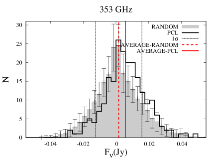
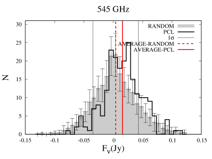
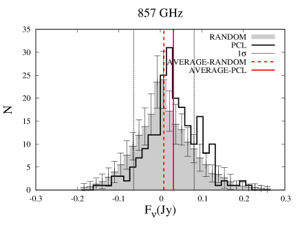
Figure 2: Top: Black solid line shows the distribution of the flux densities at 353 GHz measured at the protoclusters at $z\sim 3.8$. The gray histogram and its error show the average and standard deviation of the flux distribution of the random sky positions. The vertical dotted lines show the $1\sigma$ rms noise at 353 GHz. The red vertical solid and dashed lines show the average value of the protoclusters and random sky positions, respectively. The Middle and bottom are similar to the top panel but at 545 and 857 GHz, respectively.

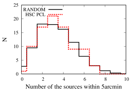
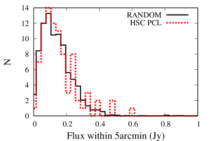
Figure 3: Top: The distribution of the number count of the $4\sigma$ sources at 250 $\mu$m within the 5-arcmin diameter aperture of the protoclusters (red dashed) and random sky positions (black solid). Bottom: Similar to the top panel but the $x$-axis shows the sum of the fluxes of the sources within 5-arcmin diameter.

3 Method

3.1 Discrete detections of the protoclusters using Planck

First, whether protoclusters are individually detected on Planck images is assessed because e.g., Greenslade et al. (2018) suggests that the most actively star-bursting protoclusters can be detected on $Planck$. At the least, none of the protoclusters matches the the second Planck compact source catalog (Planck collaboration XXXIX, 2016), a secure catalog with high detection significance and a S/N $\hskip 3.00003pt\raisebox{1.72218pt}{$>$}\raisebox{-3.01385pt}{$\sim$}\hskip 3.00003pt5$. To investigate the presence of fainter sources, the distribution of 5-arcmin diameter aperture flux values measured at the protoclusters and random sky positions shown in Fig. 2 are compared. The flux distribution for random sky positions shows the average and $1\sigma$ standard deviation of the flux distributions of 216 random sky positions measured by a thousand times iteration. The vertical dotted lines show $\pm 1\sigma$ errors. The average fluxes of the protoclusters and random sky positions are indicated with red thick solid and dashed lines, respectively. The flux distributions of the protoclusters and random points are compared via the Kolmogorov-Smirnov (KS)-test, and $p$-values $=0.006$, 0.049, and 0.778 are obtained at 353, 545, and 857 GHz, respectively. Thus, the flux distributions at 353 and 545 GHz are significantly offset from the random points. In addition, the centers of the flux distributions of the protoclusters shift brighter than those of random sky positions. The average fluxes at 353, 545, and 857 GHz are 6, 16, and 32 mJy, respectively, for the protoclusters and 2, 4, and 9 mJy for random sky positions. These excesses follow well the fluxes of the protoclusters measured using the stacking analysis.

3.2 Notes for the possibility to detect individual galaxies in the protoclusters

$H$-ATLAS and WISE are sufficiently sensitive to detect the most luminous objects at $z\sim 4$. $H$-ATLAS can detect a very bright SMG or a dense group of bright SMGs as a point source at $z\sim 4$ (e.g., Miller et al. 2018). Fan et al. (2018) and Toba et al. (2018) reported extremely IR luminous dust obscured galaxies (DOGs) at $z\sim 4$ detectable using WISE. Although such sources are quite rare, the possibility cannot be ignored that the protoclusters contain such sources detectable using Herschel and/or WISE.

The number count and total fluxes of the sources detected at the protoclusters and random sky positions are compared using the $H$-ATLAS source catalog (Valiante et al., 2016) in Fig. 3. The top panel shows the distributions of the number count of the objects detected above $4\sigma$ in 250 $\mu$m within a 5-arcmin diameter of the protoclusters and random sky positions. The bottom panel is similar to the top panel except for the sum of their fluxes. The number and flux distributions of the protoclusters and random points are compared via KS-test and $p$-values $=0.86$ and 0.84 are found, respectively. Thus, there is no significant difference between the protoclusters and random sky positions. Similarly, there is no clear difference at 350 $\mu$m and 500 $\mu$m, and also WISE $W3$ and $W4$. However, there remains still a possibility that some extremely luminous protocluster members can be found using more detailed SED analysis of the sources detected on the $H$-ATLAS and/or WISE images. This is beyond the scope of this work and will be the subject of a future paper.

3.3 Stacking analysis using WISE, IRAS, AKARI and Planck images

Next, we perform a stacking analysis of the protoclusters. Before performing the stacking analysis, we check contamination of bright foreground sources, subtract sky and smooth images. First, possible contaminants are assessed. Foreground objects can be resolved and detected on $AKARI$ images. Using SExtractor (Bertin & Arnouts, 1996), one or two sources with $1\sim 3$ Jy are detected in more than one bandpass at two fields. Because both of the fields have no corresponding source on the $H$-ATLAS images at 100 and 160 $\mu$m, the sources are not foreground objects but likely noise. To make sure, these fields are not used. The other possible bright interlopers are QSOs. Not only QSOs themselves but also possible protoclusters around them at different redshifts can contaminate the signal from our targets. Approximately one-half of the protoclusters in our catalog are within 5 arcmin of the QSOs at all redshifts selected from Sloan Digital Sky Survey (SDSS). The effect of these QSOs is checked by performing a stacking analysis rejecting such fields. Because this rejection causes no change in the results, they are not rejected. Given the aforementioned, there is no possible bright foreground interlopers at the sky positions of our targets.

We perform our own sky subtraction because the background sky levels on the archival $AKARI$, $IRAS$ and $WISE$ images considerably vary among the survey area of the protoclusters while they are nearly uniform on the Planck CIB map and $H$-ATLAS RAW images. For example, in the case of $AKARI$ $WideL$, the average sky values on the archived images at the protoclusters vary from $0.01-0.04$ Jy/pix. Thus, before stacking the images, sky subtractions for $AKARI$, $IRAS$ and $WISE$ images are performed. The archived $WISE$, $AKARI$, and $IRAS$ images are provided as 1.6 $\times$ 1.6 deg, 6 $\times$ 6 deg, and 12.4 $\times$ 12.4 deg cutouts, respectively. We evaluate the sky values on an image after masking the bright sources. To generate object masks, we extract sources using SExtractor (Bertin & Arnouts, 1996). The sources detected above $2\sigma$ for a square of the FWHM of the PSF size region, and their surrounding regions for the FWHM of the PSF size radius, are masked. The sky is evaluated with $\approx 10$ arcmin mesh and the sky images are generated. Then, the sky image is subtracted from the original image. The sky subtraction is visually assessed to ensure it works well. Though sky subtraction does not work well around very bright objects, sky subtraction at protoclusters largely works well.

Then, we smooth the sky subtracted images such that the FWHM of the PSF $\approx 4.9$ arcmin, similar to that on the Planck 353-GHz image. We cut out the images at the protoclusters taking the density peaks of the $g$-dropout galaxies as the centers. Then, we perform average stacking with 3$\sigma$ clippings by using the imcombine task of IRAF. If there are no value pixels at the edge of a cutout image, these pixels are ignored. In addition to all the protoclusters, we also perform the stacking analysis for the brighter-half protoclusters on the Planck 857-GHz image (see Fig. 2) and the protoclusters with the overdensity significances of the $g$-dropout galaxies $5\sigma$ or more. The number of the cutout images of the brighter-half protoclusters is $N=106$, rejecting the two poor $AKARI$ fields, and that of the $5\sigma$ overdense protoclusters is $N=67$. We perform 4-arcmin diameter aperture photometries and later convert them to the total fluxes by aperture correction. The average fluxes and their errors are the average and standard deviations measured via a thousand-times bootstrap resampling. The standard deviation does not only originate in the sky noise but also in the variation in the protoclusters. Finally, we apply an aperture correction to convert them into total fluxes measured in the next section.

The $1\sigma$ sky noises expected for the stacked images are listed in Table 6. They are the standard deviations of the flux values in 4-arcmin diameter apertures measured on a thousand images generated by stacking the images at 214 random sky positions. The detection limits of Planck stacks are deeper than that of the $H$-ATLAS stacks. Notably, when the HSC-SSP WIDE survey is completed, a $\sim 10$ times larger catalog will be available. Then, these stacks will be three times deeper than the current depth in the future.

We match the PSF sizes on images by a simple Gaussian smoothing; however, the PSFs on the images used here are not simply similar to a Gaussian profile. The beam profiles on the Planck images depend on the sky positions. We evaluate the average beam profile of the protoclusters in 353 GHz based on the public data-base (Planck collaboration VI, 2014). For the averaged beam profile, $\approx 62\%$, $79\%$, and $96\%$ of the total flux of a point source is enclosed in 4-, 5-, and 10-arcmin diameter apertures, respectively. For a Gaussian profile with FWHM of the PSF size $=4.9$ arcmin, $\approx 43\%$, $58\%$, and $96\%$ of the total flux of a point source is enclosed in 4-, 5-, and 10-arcmin diameter apertures, respectively. The PSFs on the $IRAS$ images are not the same as those on the $Planck$ images. Because a large Gaussian smoothing is applied on the AKARI, WISE, and Herschel images, their PSFs may not behave like Planck but a Gaussian profile. This can result in a slight inconsistency of the flux measured with different facilities. Practically, protoclusters should not behave similar to a point source. The average spatial extent of the protoclusters is measured using $H$-ATLAS in the next subsection. The average radial profile of the protoclusters in $Planck$ compared to that of the PSF and several mock source distributions are presented in Appendix B.

3.4 Stacking analysis of $H$-ATLAS images

We stack $H$-ATLAS RAW images and those smoothed to have a FWHM of the PSF sizes similar to those of a Planck image at 353 GHz. With the former products, the average physical extent and total flux of the protoclusters are limited while the fluxes measured on $Planck$ images are smoothed off because of the large PSFs and extended geometries of the protoclusters. Fig. 4 shows the average radial profiles of the protoclusters measured at 250, 350, and 500 $\mu$m. Signals of the protoclusters are detected within $\approx 4$ arcmin. For the brighter-half protoclusters, signals are detected within $\approx 6$ arcmin. We adopt the fluxes measured at an 8-arcmin diameter (12-arcmin for the brighter-half) as the lower limits of the total fluxes.

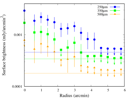
Figure 4: Average radial profile of all protoclusters measured using $Herschel$. The blue circles, green squares and yellow triangles show the average radial profiles at 250, 350, and 500 $\mu$m, respectively. The vertical lines denote the $1\sigma$ sky noise levels measured in 1 arcmin square regions. Here after, a $2\sigma$ upper limit value is shown if a signal is not detected above $2\sigma$ significance.

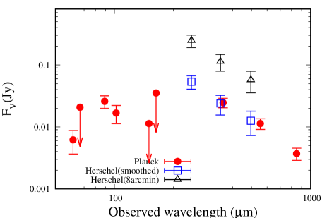
Figure 5: The red filled circles show the fluxes measured on the stacked images of Planck, AKARI, and IRAS. The blue open squares show the fluxes measured on the stacked images of the Herschel images smoothed to match the PSF sizes with those of Planck at 353 GHz. For these two, we perform 4-arcmin diameter aperture photometries. The black open triangles show the fluxes measured using an 8-arcmin diameter aperture on the stacked images of the Herschel images without smoothing.

The black triangles and blue squares in Fig. 5 show the total fluxes measured by stacking $Herschel$ images and 4-arcmin diameter aperture fluxes measured by stacking $Herschel$ images matched the PSF sizes to $Planck$ 353 GHz, respectively. The fluxes measured using the PSF-matched $Herschel$ images match quite well those measured using $Planck$ images. The average flux ratios are $4.7\pm 2.2$ and $6.6\pm 2.1$ for all and the brighter-half protoclusters, respectively. Here, these ratios are adopted as the aperture correction factors. For the $5\sigma$ overdensity protoclusters, we apply the aperture correction factor for all protoclusters. The aperture correction factors for various source geometries expected for protoclusters are simulated as presented in Appendix B. These aperture correction factors are consistent with those of the simulated protocluster geometries.

We note that background subtracted products (BACKSUB) of $H$-ATLAS are not suitable for the stacking analysis of the protoclusters because the fluxes of our targets are greatly reduced as a consequence of their sky subtraction. For example, at 250 $\mu$m, the flux of the protoclusters measured using RAW images is two times greater than that using BACKSUB images. This result is perhaps because sky subtraction is performed at a scale smaller than the typical extent of the protoclusters and the subtracted sky values are similar to the protoclusters fluxes. The difference between the BACKSUB and RAW images is less ($<10\%$) for $g$-dropout galaxies and QSOs (Section 3.6) because they are point sources and $g$-dropout galaxies are much fainter than protoclusters.

3.5 Average optical total fluxes

Because the contamination of nearby sources is large, we avoid a stacking analysis in optical. We here limit the average total fluxes of the protocluster galaxies in the $g,r,i,z\&y$-band by summing the Cmodel fluxes of the $g$-dropout galaxies in the HSC-SSP catalog public data release 1 (pdr1: Aihara et al. 2018). First, the average total fluxes of the $g$-dropout galaxies with a $i\leq 25.0$ mag within the 8-arcmin diameter of the protoclusters is measured and that of 1000 random positions. Then, the latter is subtracted from the former. Note that this is a lower limit because the contribution from the galaxies with $i>25.0$ mag are ignored.

3.6 Stacking analysis of the $g$-dropout galaxies and SDSS QSOs

To discuss whether the optically selected objects can explain the entire flux of the protoclusters, we perform stacking analyses of $g$-dropout galaxies and SDSS QSOs. Approximately $\approx 238,500$ ($\approx 94,000$ for $H$-ATLAS) $g$-dropout galaxies with an $i\leq 25.0$ are used but not within 10 arcmin of the protoclusters from the HSC-SSP survey area in Toshikawa et al. (2018). We also use 151 (60 in $H$-ATLAS) SDSS QSOs at $3.3<z<4.2$ studied in Uchiyama et al. (2018) which shows that only two out of the 151 QSOs reside in the protoclusters selected by Toshikawa et al. (2018).

To obtain the average flux as that from a single object, it is ideal to stack only isolated sources and measure flux on PSF matched images with a sufficiently large aperture; however, the PSFs of the images used here are extremely large to use such a robust method. We here stack them without any smoothing. The fluxes measured with $2\times$ FWHM of the PSF aperture diameter on each image are adopted as approximate estimates of the total fluxes. Notably, contaminations from other sources are not likely negligible even for $WISE$ and $Herschel$, and are considerably large for $IRAS$, $AKARI$, and $Planck$ images.

As the $g,~{}r,~{}i,~{}z~{}\&~{}y$-band flux values and errors, the median and standard deviation of the Cmodel fluxes of them from the HSC-SSP catalog pdr1 (Aihara et al., 2018) are used.

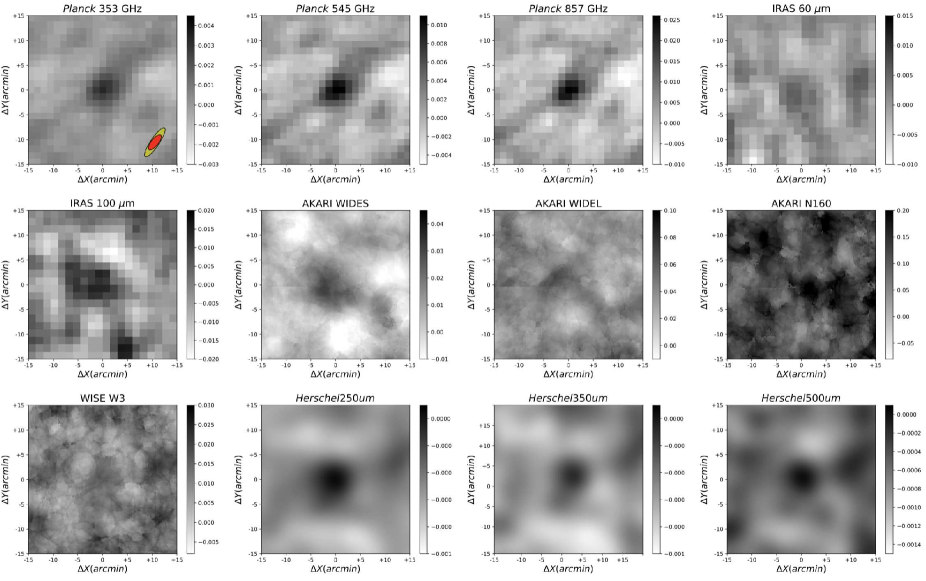
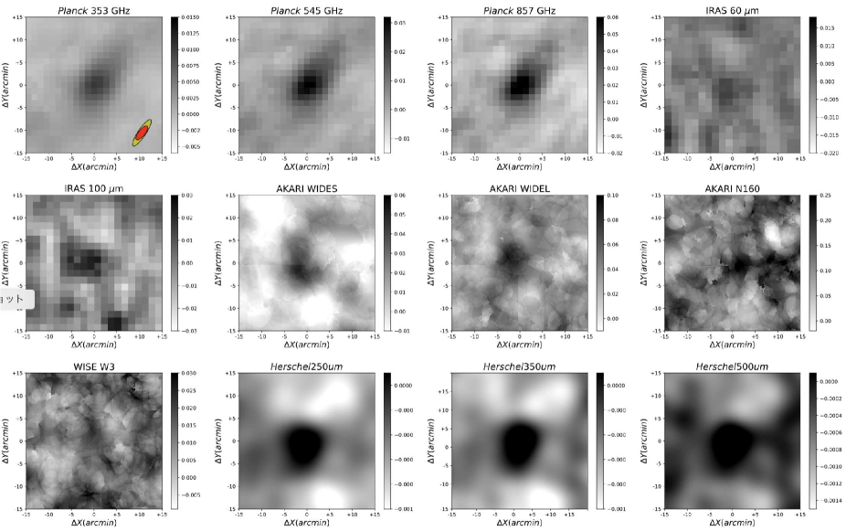
Figure 6: Stacked images of the protoclusters in Planck 353, 545, and 857 GHz; IRAS 60 and 100 $\mu$m; AKARI WIDES, WIDEL, and N160; WISE W3;, and Hershcel 250, 350, and 500 $\mu$m from the top left to bottom right. All the images are 30 arcmin by side. The ellipses on the 353-GHz images show the average beam profiles described in Section 3.3. In the case of a point source, 50% and 90% of fluxes are included within the red and yellow-filled ellipses, respectively.

Figure 6: - continues. The stacked images of the brighter-half protoclusters.

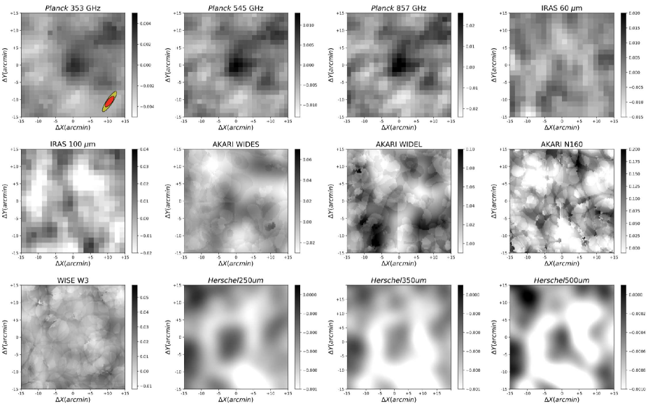
Figure 6: - continues. The stacked images of $5\sigma$ overdensity protoclusters.

Table 1: The flux densities of HSC SSP $g$-dropout protoclusters

	IRAS		Planck			Herschel
Sample	60 $\mu$m	100 $\mu$m	857 GHz	545 GHz	353 GHz	250 $\mu$m	350 $\mu$m	500 $\mu$m
			(350 $\mu$m)	(540 $\mu$m)	(840 $\mu$m)
	(mJy)	(mJy)	(mJy)	(mJy)	(mJy)	(mJy)	(mJy)	(mJy)
All	$6.2\pm 2.5$	$16.8\pm 5.5$	$24.7\pm 4.3$	$11.3\pm 2.2$	$3.7\pm 0.8$	$53.8\pm 13.3$	$24.0\pm 8.4$	$12.6\pm 5.3$
Brighter-half	$8.9\pm 3.6$	$23.3\pm 9.4$	$69.6\pm 4.2$	$33.8\pm 2.2$	$11.6\pm 0.9$	$96.2\pm 19.8$	$58.2\pm 11.6$	$35.4\pm 9.1$
$5\sigma$ overdensity	$<7.9$	$14.7\pm 6.7$	$27.0\pm 6.3$	$11.8\pm 3.2$	$3.5\pm 1.2$	$45.3\pm 14.3$	$<26.9$	$<15.1$

Note. — Flux values are measured in 4-arcmin diameter aperture. Each flux and error are the average and standard deviation of a thousand times bootstrap resampling. If they are not detected above 2$\sigma$, we put a 2$\sigma$ value as an upper limit.

Table 2: –continues

	AKARI				WISE
Sample	N60	WIDE-S	WIDE-L	N160	W1	W2	W3	W4
	(65 $\mu$m)	(90 $\mu$m)	(140 $\mu$m)	(160 $\mu$m)	(3.4 $\mu$m)	(4.6 $\mu$m)	(12 $\mu$m)	(22 $\mu$m)
	(mJy)	(mJy)	(mJy)	(mJy)	(mJy)	(mJy)	(mJy)	(mJy)
All	$<41.5$	$25.9\pm 5.9$	$<22.7$	$<70.6$	$<0.82$	$<0.57$	$0.40\pm 0.13$	$<0.57$
Brighter-half	$<58.5$	$43.8\pm 8.2$	$67.1\pm 16.8$	$106.4\pm 49.9$	$<0.98$	$<0.57$	$0.54\pm 0.18$	$<0.86$
$5\sigma$ overdensity	$<77.6$	$23.2\pm 9.7$	$<40.5$	$<118.5$	$<1.84$	$<0.92$	$<0.56$	$<1.28$

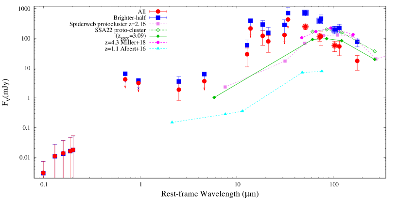
Figure 7: SEDs of the protoclusters at $z=3.8$ and the known protoclusters. The red filled circles and blue filled squares show all and the brighter-half protoclusters. The encircled symbols show that measured with $H$-ATLAS. We show the sum of the IR sources in the known protoclusters within the same physical size (8 arcmin $\approx 3.4$ physical Mpc diameter). We scale all of them to be at $z=3.8$. The violet filled squares with a dashed line show the Spiderweb protocluster at $z=2.16$ based on Dannerbauer et al. (2014). The green open diamonds with a dotted line is the SSA22 protocluster at $z\approx 3.09$ based on Kato et al. (2016) and Umehata et al. (2014). The green filled diamonds with a solid line is that limit to $z_{\rm spec}\approx 3.09$ (Umehata et al., 2018). The data point at 6 $\mu$m is the sum of the fluxes of sources at $z_{\rm spec}\approx 3.09$ in Umehata et al. (2018) measured with Spitzer MIPS 24 $\mu$m image in archive (Webb et al., 2009). The magenta filled pentagons with a dashed line are a protocluster at $z=4.3$ in Miller et al. (2018). The cyan filled triangles with a dashed line are a protocluster at $z=1.1$ in Alberts et al. (2016).

4 Result

Figure 6 shows the stacked images of all, brighter-half, and 5$\sigma$-overdensity protoclusters. Table 1 summarizes their fluxes measured using a 4-arcmin diameter aperture. Signals are significantly detected in WISE $W3$; IRAS 60 and 100 $\mu$m; AKARI WIDES (and WIDEL and N160 for the brighter-half); Planck 353, 545, and 857 GHz, and $Herschel$ 250, 350, and 500 $\mu$m. Although the spectroscopic follow-up of the protoclusters remains on-going, it is shown that they trace special environments with excess IR emission. Fig. 7 shows the SEDs in the total flux obtained by multiplying the aperture fluxes using the aperture correction factors found in Section 3.4. This is the first time the “average” SED of a protocluster is shown.

The flux values of all and the 5$\sigma$-overdensity protoclusters are identical although 5$\sigma$ is a more reliable overdensity threshold. It implies that the 4$\sigma$ selection is as reliable as the 5$\sigma$ selection of the protoclusters. The brighter-half protoclusters are twice brighter in the Planck than all the protoclusters while there is no significant difference in the optical. This implies that above the $4\sigma$ overdensity threshold, there is no strong correlation between the optical and IR properties on average. Our study demonstrates that deep multi-wavelength observations are necessary to characterize protoclusters.

Fig. 2 and 2 in Appendix C show the stacked images of the 1st and 2nd quartiles from the lowest of the flux distribution at 857 GHz (Fig. 2). The 2nd quartile is marginally detected while the 1st quartile shows negative detections perhaps because of noise. This indicates the possibility of the artificial signal on the $Planck$ HFI images. However, because the $Herschel$ and $Planck$ results match quite well (Fig. 5), they should be negligible.

In the followings, our results are compared to the known protoclusters at various redshifts and various populations at $z\sim 4$.

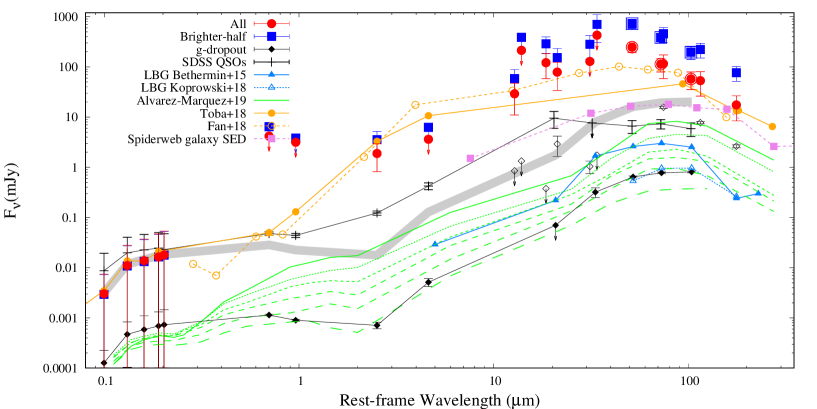
Figure 8: Similar to Fig.7 but we compare with various galaxies at $z\sim 4$. The black filled diamonds with a solid line show the average flux of a $g$-dropout galaxy measured in Section 3.6. Those measured in $Planck$, $AKARI$, and $IRAS$ are shown with open symbols since they are severely contaminated by their neighbor sources. The black crosses with a solid line show the average flux of a SDSS QSO at $z\sim 4$ measured in Section 3.6. The light blue filled triangles with a solid line and open triangles with a dot line show the average flux of a typical SFG at $z\sim 4$ in Béthermin et al. (2015) and Koprowski et al. (2018), respectively. The green curves show the average fluxes of LBGs at $z\sim 3$ split by stellar mass in Álvarez-Márquez et al. (2019), scaled at $z=3.8$. The orange filled circles with a solid line and open circles with a dashed line show infrared luminous DOGs at $z=3.7$ in Toba et al. (2018) and at $z=4.6$ in Fan et al. (2018) scaled at $z=3.8$, respectively. The violet filled squares with a dashed line show the SED of the HzRG in the Spiderweb protocluster (Dannerbauer et al., 2014). The gray shaded region shows the SEDs of the $g$-dropout galaxies multiplied by 20 to 30.

4.1 Comparison to the known protoclusters

First, we compare our results with the known protoclusters deeply observed in far-infrared (FIR) in Fig. 7. We show the sum of the fluxes of the IR sources at the same physical size (8 arcmin $\approx$ 3.4 physical Mpc diameter) of the Spiderweb (MRC1138-262) protocluster at $z=2.16$ (Dannerbauer et al., 2014), the SSA22 protocluster at $z=3.09$ (Webb et al., 2009; Kato et al., 2016; Umehata et al., 2018), a protocluster at $z=4.3$ reported in Miller et al. (2018) and a massive cluster at $z=1.1$ in Alberts et al. (2016). The IR sources in the protoclusters at $z>2$ are selected as sub-mm sources while those in Alberts et al. (2016) are selected at 100 $\mu$m. The fluxes of the objects with spectroscopic redshifts $z_{\rm spec}$ and/or photometric redshifts $z_{\rm phot}$ similar to the protoclusters are summed. The sum of the purely spectroscopically confirmed sources for the SSA22 protocluster is also shown. Their fluxes are scaled to be at $z=3.8$ by multiplying with (1+3.8)/$(1+z_{\rm at~{}known~{}(proto)cluster})\times(D_{\rm L~{}at~{}known~{}(proto)cluster})^{2}/(D_{\rm L~{}at~{}z=3.8})^{2}$ where $D_{\rm L}$ is the luminosity distance. Note that only the sources brighter than ultra-luminous infrared galaxies (ULIRGs) or hyper-luminous infrared galaxies (HyLIRGs) are counted in the known protoclusters at $z>2$ ($\hskip 3.00003pt\raisebox{1.72218pt}{$>$}\raisebox{-3.01385pt}{$\sim$}\hskip 3.00003pt4$ mJy at 850 $\mu$m for Spiderweb and $\hskip 3.00003pt\raisebox{1.72218pt}{$>$}\raisebox{-3.01385pt}{$\sim$}\hskip 3.00003pt0.4$ mJy at 1.1 mm for SSA22). In the case of the SSA22 protocluster, the detections of the $X$-ray selected AGNs at $z_{\rm spec}\approx 3.09$ (Lehmer et al., 2009; Kubo et al., 2015) in 24 $\mu$m are also checked. All the 24 $\mu$m detected AGNs are already included in the sum shown in Fig. 7.

At $>100~{}\mu$m in the rest-frame, the flux from the protoclusters at $z\sim 3.8$ and the known protoclusters at $z=2-4$ do not differ in order. Amazingly, the Spiderweb and SSA22 protoclusters are just as luminous as the typical massive protoclusters at $z\sim 3.8$ though they have been believed to be the most prominent structures at $z=2-3$. In addition, the SEDs of the Spiderweb and SSA22 protoclusters more rapidly decrease at $<100~{}\mu$m than those of the protoclusters at $z\sim 3.8$. Although only the bright sources in the known protoclusters are summed, this tendency may not appreciably change by adding the fluxes from IR faint sources optically detected (Section 4.2 and 5). Our results imply that the Spiderweb and SSA22 protoclusters may not be particularly special protoclusters in the IR, and/or the typical IR luminosities and SEDs of the protoclusters have changed drastically between $z=2$ and 4.

4.2 Comparison to LBGs, SDSS QSOs and infrared luminous DOGs at $z\sim 4$

Next, we compare the SEDs of the protoclusters with those of typical SFGs (Béthermin et al. 2015; Koprowski et al. 2018 and $g$-dropout galaxies from the HSC-SSP survey) and IR luminous DOGs (Fan et al., 2018; Toba et al., 2018) at $z\sim 4$ in Fig. 8.

The blue filled and open triangles in Fig. 8 show the average SEDs of typical SFGs at $z\sim 4$ measured by stacking analysis in Béthermin et al. (2015) and Koprowski et al. (2018). The green curves show LBGs at $z=3$ split by stellar mass in Álvarez-Márquez et al. (2019), scaled at $z=3.8$. The black diamonds show the average SED of the $g$-dropout galaxies with an $i\leq 25.0$ mag in the HSC-SSP survey obtained in Section 3.6. The $Planck$, $AKARI$, and $IRAS$ fluxes shown with open symbols deviate from $Herschel$ and $WISE$. These may be contaminated by surrounding $g$-dropout galaxies as well as some unknown protoclusters because of low spatial resolution. The average SED of the $g$-dropout galaxies selected from the HSC-SSP survey matches well Koprowski et al. (2018) and Álvarez-Márquez et al. (2019) whose sample selections are similar to ours. Béthermin et al. (2015) is biased to more massive objects and there is no wonder that it does not match our results. The gray shaded region shows the SED of $g$-dropout galaxies multiplied by 20 to 30 which is the expected number of $g$-dropout galaxies with an $i\leq 25$ mag in a protocluster. The protoclusters are not only several tens of times brighter than typical SFGs but they have SEDs with greater warm/hot dust component compared to those of typical SFGs at $z\sim 4$. From the aforementioned, we argue that the IR SEDs of the protoclusters cannot be explained by only multiplying typical SFGs at $z\sim 4$.

The dust torus of an AGN are luminous in the mid to FIR; however, at least, SDSS QSOs or optically luminous QSOs are not found at the HSC-SSP protoclusters in general (Uchiyama et al., 2018). Our results suggests that there are overdensities of IR sources that cannot be selected by $g$-dropout selection and/or $g$-dropout galaxies in the protoclusters have special properties such as AGN-dominated DOGs; The extremely IR luminous DOGs detectable with $WISE$ at $z=3.7$ (Toba et al., 2018) and at $z=4.6$ (Fan et al., 2018) are shown in Fig. 8. Toba et al. (2018) is shown without any scaling while Fan et al. (2018) is plotted after scaling the flux at $z=3.8$. Interestingly, the SEDs of the protoclusters quite resemble those of the luminous DOGs. They report that these DOGs have IR SEDs dominated by dust emission from AGN tori. Because the AGN emission dominates $\sim 50$ % of the total flux even at $\sim 200~{}\mu$m in the rest-frame, despite the huge total IR luminosity, these DOGs have a SFR of only $\sim 480$ and 1300 $M_{\odot}$ yr^-1 for Fan et al. (2018) and Toba et al. (2018), respectively. This result implies that dust emission from AGN tori and moreover a single object such as IR luminous DOGs can dominate the fluxes of the protoclusters.

We discuss the breakdown of the IR emission from the protoclusters by fitting them with models as in the next section.

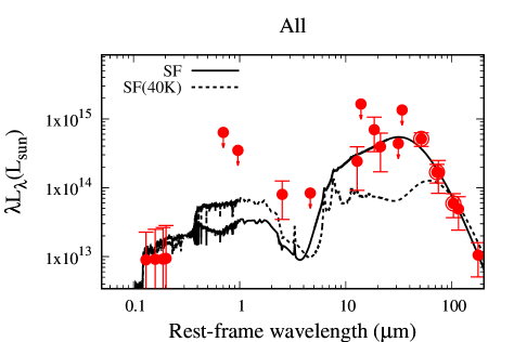
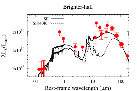
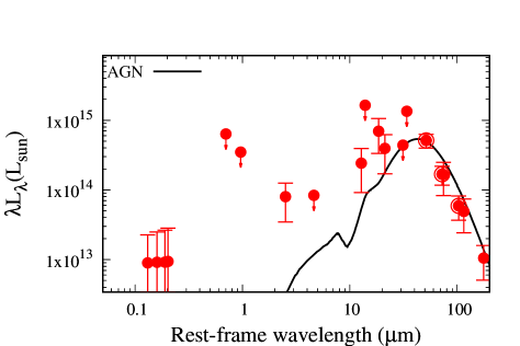
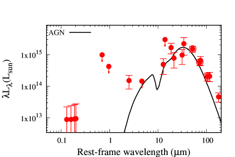
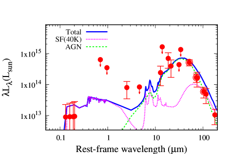
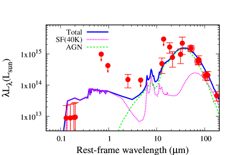
Figure 9: Left: Best-fit SEDs for all the protoclusters. The red filled circles show the observed fluxes. Left top: The black solid curve shows the best-fit SED found with MAGPHYS. The black dashed curve shows the best-fit SED found with MAGPHYS limit to $T_{dust}\approx 40~{}K$. Left middle: The black solid line shows the best-fit SED for AGN SED models. Left bottom: The best-fit model for composite SED models of a MAGPHYS and an AGN SED model. The blue solid, magenta dotted, and green dashed lines show the total, star-forming, and AGN components of the best-fit SEDs, respectively. Right: Similar to the left panels but for the brighter-half protoclusters.

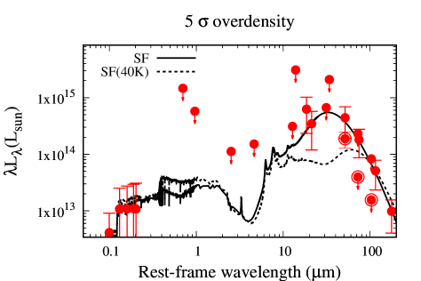
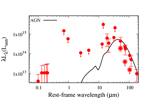
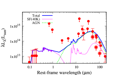
Figure 9: –continues. Similar to the above figures of Fig. 9 but for the 5$\sigma$ overdensity protoclusters.

Table 3: $\chi^{2}/\nu$ values for SED models

Sample	MAGPHYS	MAGPHYS ($T_{dust}=40K$)	AGN	MAGPHYS+AGN
All	0.53	2.50	0.74	0.62
Brighter-half	0.76	3.60	1.50	0.91
$>5\sigma$ overdensity	0.55	1.46	0.55	0.46

Table 4: Best fit SED model (model: MAGPHYS ($T_{dust}=40K$) + AGN)

Sample	$L_{FIR,SB}$	$L_{FIR,AGN}$	$L_{FIR,total}$	$L_{FIR,SB}/L_{FIR,AGN}$	SFR	$A_{V}$
	($10^{13}~{}L_{\odot}$)	($10^{13}~{}L_{\odot}$)	($10^{13}~{}L_{\odot}$)		($10^{3}~{}M_{\odot}$ yr-1 )
All	$1.3_{-1.0}^{+1.6}$	$3.7_{-2.0}^{+1.8}$	$5.1_{-2.5}^{+2.5}$	$0.4^{+0.7}_{-0.2}$	$2.1^{+6.3}_{-1.7}$	$0.5^{+1.0}_{-0.2}$
Brighter-half	$3.2_{-1.0}^{+4.5}$	$11.1_{-3.6}^{+3.5}$	$14.2_{-4.5}^{+5.8}$	$0.3^{+0.5}_{-0.0}$	$1.9^{+3.9}_{-0.9}$	$1.0^{+0.0}_{-0.4}$
$>5\sigma$ overdensity	$0.9_{-0.8}^{+1.4}$	$2.8_{-2.3}^{+1.7}$	$3.7_{-2.9}^{+2.1}$	$0.3^{+1.8}_{-0.3}$	$1.1^{+2.9}_{-1.0}$	$0.3^{+1.8}_{-0.0}$

Table 5: Best fit SED model (model: MAGPHYS)

Sample	$T_{dust}$	$L_{dust}$	SFR	$A_{V}$
		($10^{13}~{}L_{\odot}$)	($10^{3}~{}M_{\odot}$ yr-1 )
All	$71_{-2}^{+4}$	$19.3_{-4.2}^{+0.6}$	$16.3_{-7.8}^{+1.0}$	$1.7^{+1.6}_{-0.1}$
Brighter-half	$74_{-12}^{+0}$	$48.7_{-7.1}^{+0.7}$	$43.4_{-8.2}^{+2.9}$	$1.8^{+1.9}_{-0.0}$
$>5\sigma$ overdensity	$75_{-20}^{+0}$	$16.0_{-11.7}^{+8.2}$	$13.4_{-10.1}^{+6.9}$	$1.7^{+3.4}_{-0.4}$

5 Discussion

5.1 Origin of the IR emission

First, the sum of the IR fluxes of the $g$-dropout galaxies of the protoclusters, estimated by multiplying the average flux of a $g$-dropout galaxy with the number excess of $g$-dropout galaxies ($N=20\sim 30$), is only a third and a tenth of the flux of all and the brighter-half protoclusters, respectively. In addition, the average SED of the $g$-dropout galaxies is different from that of the protoclusters. Therefore the $g$-dropout galaxies are not sufficient to explain the whole IR flux of the protoclusters. Obscured AGNs are plausible origin of the MIR excess (Fan et al., 2018; Toba et al., 2018). According to the previous studies of the protoclusters shown in Fig. 7, several SMGs comprise the remaining greater portion of the IR luminosity of the protoclusters. It is also reported that such sources found by single-dish telescopes are resolved into multiple SMGs by ALMA (e.g., Umehata et al. 2018).

We discuss the origin of the IR emission of the protoclusters by fitting the observed SEDs with the model SEDs. The major components of a SED from $\approx 0.01$ to $200~{}\mu$m in the rest-frame are stellar emission, and emission from dust heated by young stars and AGN torus (Here we ignore other AGN components since we focus on the dust emission in the IR). Therefore, the SED fitting is performed by using the models of (1) stellar emission and emission from dust heated by stars, (2) AGN torus, and (3) their combination.

We adopt the SED models from MAGPHYS (da Cunha et al., 2008) which generates the SED models via the combinations of stellar light and emission from dust heated by young stars. MAGPHYS describes the UV to IR SEDs with the consistency of the absorbed UV light and that re-emitted in IR. The dust in MAGPHYS consists of that in stellar birth clouds and ambient inter-stellar medium. The former represents hot ($130-250~{}K$) and warm ($30-60~{}K$) dust components, and the latter represents a cold ($15-25~{}K$) dust component. Notably, MAGPHYS can generate a model containing a large warm/hot dust component which can also originate in an AGN torus. MAGPHYS is a comprehensive package generating various SED models and fitting an observed SED with SED models. When combining MAGPHYS models with AGN models, we extract $\approx 4800$ models with solar metallicity and dust temperature $T_{dust}\approx 40~{}K$ (for SFGs at $z\sim 4$ in Koprowski et al. 2018) for simplification.

For SED models of AGNs, we adopt the model library by Siebenmorgen et al. (2015). Their models are parameterized by viewing angle, inner radius of the dusty torus $R$, cloud volume filling factor $V_{c}$, optical depth (in $V$-band) of the individual clouds $A_{c}$ and the optical depth (in $V$-band) of the disk mid-plane $A_{d}$. Because the images are stacked, we use the average of the model SEDs with the same parameters but different viewing angles. The Lyman forest absorption at $\lambda<1216$ Å  in the rest-frame is manually added on AGN models following Madau (1995).

Then we fit the observed SEDs in case (1) to (3) using a standard $\chi^{2}$ minimization procedure. In case (3), we fit the observed SEDs with the models combining SFG and AGN models with free ratio. Fig. 9 shows the best-fit SED models and Table 3 shows their $\chi^{2}/\nu$ values. The $\chi^{2}/\nu$ values minimize for cases (1) and (3). The best-fit SED parameters are shown in Table 4 and 5. Though several works suggested high dust temperatures for SFGs at high redshift (e.g., Magdis et al. 2012; Béthermin et al. 2015; Bouwens et al. 2016; Faisst et al. 2017; Liang et al. 2019), the best-fit models of MAGPHYS of protoclusters have dust temperatures $T_{dust}\sim 70~{}K$, which are exceptionally higher than that of a typical SFG at $z\sim 4$, $T_{dust}\sim 40~{}K$ (Koprowski et al., 2018). Such high $T_{dust}$ models describe SFGs with a very high specific SFR $\hskip 3.00003pt\raisebox{1.72218pt}{$>$}\raisebox{-3.01385pt}{$\sim$}\hskip 3.00003pt10$ Gyr^-1. In the case of the composite models, $70\sim 80~{}\%$ of the total FIR ($8-1000~{}\mu$m) luminosities originate in AGNs. Briefly, the total FIR luminosity of all and the brighter-half protoclusters is $5.1_{-2.5}^{+2.5}$ and $14.2_{-4.5}^{+5.8}\times 10^{13}~{}L_{\odot}$, respectively for the best-fit MAGPHYS+AGN models and $19.3_{-4.2}^{+0.6}$ and $48.7_{-7.1}^{+0.7}\times 10^{13}~{}L_{\odot}$, respectively, for the best-fit MAGPHYS models. The total SFR of all and the brighter-half protoclusters is $2.1_{-1.7}^{+6.3}$ and $1.9_{-0.9}^{+3.9}$ $\times 10^{3}~{}M_{\odot}$ yr^-1, respectively, for the best-fit MAGPHYS+AGN models and $16.3_{-7.8}^{+1.0}$ and $43.4_{-8.2}^{+2.9}$ $\times 10^{3}~{}M_{\odot}$ yr^-1, respectively, for the best-fit MAGPHYS models.

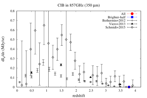
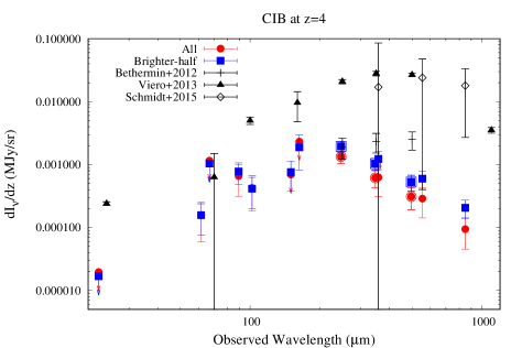
Figure 10: Left: CIB level redshift distribution in 857 GHz (350 $\mu$m). The red filled circle and blue filled square show the CIB from all and the brighter-half protoclusters, respectively. The black crosses, triangles, and diamonds show the CIB mean levels in Béthermin et al. (2012), Viero et al. (2013), and Schmidt et al. (2015), respectively. We show the median value at $3.4<z<4.0$ in Table B1 of Béthermin et al. (2012), the value at $3.0<z<4.0$ in Table 6 of Viero et al. (2013), and the median value at $3.325<z<4.225$ in Table 6 of Schmidt et al. (2015). Right: The CIB level at $z=4$. Symbols are the same as left panel.

At this point, whether the warm/hot dust emission from the protoclusters originates in star formation or AGNs cannot be determined by the SED fitting. However, given the dust temperature of typical SFGs at $z\sim 4$, and the presence of luminous QSOs and/or overdensities of AGNs in the known protoclusters at $z=2-3$, dust emission from AGNs are likely not negligible. Further characterization of galaxies in the protoclusters e.g., SEDs with higher S/N ratio and line diagnostics for individual sources will be helpful to distinguish these scenarios.

5.2 Contribution of the protoclusters to the CIB at $z\sim 4$

The cosmic infrared background (CIB; Lagache et al. 2005; Planck collaboration XVIII 2011) is the cumulative infrared emission from all galaxies/AGNs throughout cosmic history (Dole et al., 2006; Planck collaboration XXX, 2014). The redshift evolution of the mean CIB intensity is an important probe of the whole star formation history in the Universe. The anisotropy of the CIB traces the large scale distribution of DSFGs (Amblard et al., 2011; Béthermin et al., 2012, 2013; Viero et al., 2013; Maniyar et al., 2018). Protoclusters should represent the most biased regions of the CIB. Here, we discuss the consistency of our results with the CIB anisotropy studies in literatures.

Fig. 10 shows the redshift evolution of the CIB intensity at 857 GHz ($\approx 350~{}\mu$m) and the wavelength dependence of the CIB intensity at $z\sim 4$. The average flux of a protocluster is converted into the CIB intensity in MJy/sr by, $dI_{\nu}/dz=F_{\nu}~{}({\rm MJy})\times N_{\rm pcl}~{}(deg^{-2})\times 3282~{}(sr~{}deg^{-2})~{}/~{}dz$, where the number density of the protoclusters $N_{\rm pcl}~{}(deg^{-2})=179/121$ and the redshift range $dz\approx 0.9$ according to the redshift selection function for $g$-dropout galaxies in Toshikawa et al. (2016). Béthermin et al. (2012) and Viero et al. (2013) obtained the CIB intensity by stacking the $Herschel$ images of the photometric redshift catalogs. Schmidt et al. (2015) evaluated the CIB intensity based on the $Planck$ HFI data inferring redshift distribution by taking a cross-correlation with SDSS QSOs. Note that Béthermin et al. (2012) is only sensitive for the sources with 24 $\mu$m fluxes $>80\mu$Jy while Viero et al. (2013) studied sources fainter than Béthermin et al. (2012). The cross-correlation method (e.g., Schmidt et al. 2015; Maniyar et al. 2018) is sensitive for further faint unresolved populations but only covers the $Planck$ HFI bandpath at this point.

The CIB intensity at $z\sim 4$ is $0.02\sim 0.03$ MJy/sr in 857 GHz or 350 $\mu$m in the literatures (Viero et al., 2013; Schmidt et al., 2015; Maniyar et al., 2018). All protoclusters in this study have a 350 $\mu$m intensity of $0.0006\pm 0.0003$ MJy/sr while that of the brighter-half protoclusters is $0.0012\pm 0.0004$ MJy/sr. This implies that we should consider the IR luminosity function of the protoclusters to properly evaluate the protocluster contribution to the CIB. Here, we adopt the value evaluated with the brighter-half protoclusters as a lower limit. According to Maniyar et al. (2018) who evaluated the CIB anisotropy based on the $Planck$ CIB auto- and cross-power spectra, and the CIB and CMB (cosmic microwave background) lensing cross-spectra, the dark matter halos contributing the most to the CIB have a nearly constant $M_{h}\approx 10^{12.77}~{}M_{\odot}$ at $1<z<4$. According to them, the contribution of dark matter halos with $M_{h}>10^{13}~{}M_{\odot}$, which is the typical mass of the protoclusters in Toshikawa et al. (2018), to the whole CIB is several percent, although the volume density of the protoclusters at $z\sim 4$ is quite small. We find that the protoclusters in Toshikawa et al. (2018) comprise the $\hskip 3.00003pt\raisebox{1.72218pt}{$>$}\raisebox{-3.01385pt}{$\sim$}\hskip 3.00003pt6$ % of the whole CIB at $z\sim 4$, consistent with Maniyar et al. (2018).

At $<350~{}\mu$m, the contribution of the protoclusters to the entire CIB intensity becomes larger than that at a longer wavelength. This can reflect the true bias of warm dust emission sources such as AGNs and young starburst galaxies but note that there are several observational gaps.; The previous studies performed using the stacking analysis of the photometric redshift catalogs are subject to the selection incompleteness because of the survey depth and the photometric redshift selections which tend to miss objects with non-galaxy-like SEDs e.g., QSOs. The cross-power spectra method (e.g., Maniyar et al. 2018) assumes only the typical SED of SFGs. Schmidt et al. (2015) used SDSS QSOs as priors, however, they do not always represent the regions brightest in the IR (Section 5.4).

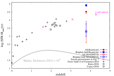
Figure 11: Evolution of the SFRs of the protoclusters. The red filled circle and blue filled square show the (average) SFR of all and the brighter-half protoclusters evaluated by multiplying $L_{FIR}$ in Table 5 with the convertion factor in Kennicutt (1998). The open ones are the SFR in Table 4 which are subtracted of the contribution of AGNs. The black crosses, open circles, and squares show the protoclusers/clusters summarized in Clements et al. (2014), Kato et al. (2016) and Casey (2016). The magenta crosses show the four protoclusters in Fig. 7. The gray tick curve shows the cosmic SFR density in general field in Madau & Dickinson (2014) multiplied by $10^{4}$.

5.3 Evolution of SFRs of massive protoclusters

Figure 11 shows the evolution of the SFR of protoclusters/clusters. At $z\sim 3.8$, we show the total SFRs subtracted of the IR emission from AGNs (Table 4) and those measured by only multiplying the total FIR luminosities (Table 5) with a conversion factor in Kennicutt (1998) where SFR $=L_{FIR}\times 1.7\times 10^{-10}~{}(M_{\odot}$ yr^-1). Our results are compared to the SFRs of massive protoclusters/clusters. We refer to the protoclusters/clusters at $0<z<3$ listed in Table 8 of Clements et al. (2014) which is originally based on Meusinger et al. (2000) (Perseus), Braglia et al. (2011) (A3112), Fadda et al. (2000) (A1689), Haines et al. (2009) (A1758). Chung et al. (2010) (the Bullet cluster), Geach et al. (2006) (Cl0024+16 and MS0451-03), Stevens et al. (2010) (protoclusters around QSOs at $1.7<z<2.8$), and clusters of DSFGs selected with $Planck$ and $Herschel$ in Clements et al. (2014); 2QZ and HS1700 protoclusters in Kato et al. (2016);. the known protoclusters shown in Fig. 7:, and the GOODS-N $z=1.99$ protocluster (Blain et al., 2004; Chapman et al., 2009), COSMOS $z=2.10$ protocluster (Yuan et al., 2014) and COSMOS $z=2.47$ protocluster (Casey et al., 2015) summarized in Casey (2016). Clements et al. (2014) measured the total IR luminosities of all the IR sources in protoclusters/clusters by fitting their IR SEDs with a modified black body with a dust emission index $\beta=2$ and converted them to the SFR with the relation in Bell (2003), which is slightly (10 percent) different from that in Kennicutt (1998). Kato et al. (2016) pre-selected IR sources with photometric redshifts, measured the IR luminosities by fitting their IR SEDs with a modified black body with a dust emission index $\beta=1.5$, and converted them to the SFR with the conversion factor in Kennicutt (1998). The SFRs summarized in Casey (2016) were measured using MAGPHYS or the conversion factor in Kennicutt (1998). For the known protoclusters shown in Fig. 7 (we use the spec-z only flux for the SSA22 protocluster), the total FIR luminosities are measured by fitting the total IR SEDs with MAGPHYS and converting them into the SFR using the conversion factor in Kennicutt (1998). Although there are differences in the methods to obtain total FIR luminosities, the SFRs converted using Kennicutt (1998) or Bell (2003) are evaluated in a similar manner.

Here, the total SFRs are shown while Clements et al. (2014) and Kato et al. (2016) showed a SFR density-redshift diagram. Because their considered sizes ($\sim 1$ Mpc in physical radius volume) of high-z protoclusters are smaller than the considered size of the protoclusters at $z=3.8$ in this study, it is not trivial to calibrate our measurement to their SFR density. Notably, according to the empirical source distributions in the known protoclusters and our simulation shown in Fig. 2, most of the fluxes from the IR sources in the protoclusters are likely concentrated within a few arcmin ($\sim 1$ Mpc in physical) radius. Thus the SFR densities of the protoclusters at the central $\sim 1$ Mpc in physical radius volume may follow the total SFRs well. At $z\hskip 3.00003pt\raisebox{1.72218pt}{$>$}\raisebox{-3.01385pt}{$\sim$}\hskip 3.00003pt2$, the literature only considers bright sources more luminous than ULIRGs/HyLIRGs. In Section 5.1, we found that one third of the flux of a protocluster can originate in $g$-dropout galaxies. The upward arrow at $z=4.3$ in Fig. 11 shows a possible correction because of such galaxies optically selected.

The measured masses of the referred $z\hskip 3.00003pt\raisebox{1.72218pt}{$<$}\raisebox{-3.01385pt}{$\sim$}\hskip 3.00003pt1$ clusters are $M_{h}=6\times 10^{14}~{}M_{\odot}$ to a few $10^{15}~{}M_{\odot}$ while those of protoclusters are approximately $10^{14}~{}M_{\odot}$. Our targets are relatively massive protoclusters which will collapse into a halo with halo mass $>10^{14}~{}M_{\odot}$. Therefore, although the selection techniques are not uniform, Fig. 11 shows the evolution of the most massive clusters today. While the cosmic SFR density in general field peaks at $z\sim 2$ (e.g., Gruppioni et al. 2013; Madau & Dickinson 2014; Bourne et al. 2017), the SFRs of the protoclusters evaluated by only multiplying the total IR luminosity by the conversion factor in Kennicutt (1998) are likely on one track which rapidly evolves at $z=0-0.5$ and continues to increase up to $z\sim 4$. However, if we subtract the emission from AGNs, the SFR of a protocluster drops at $z=3\sim 4$. The protoclusters in the literature also need the consideration of AGNs. Though not as much as AGNs, the SFR to FIR luminosity relation depends on the assumed stellar population synthesis model. It can be said that the total IR luminosity of massive protoclusters continues to increase up to $z\sim 4$; however, to show the evolution of the total SFR/SFR density, a more careful treatment of AGNs and stellar population of galaxies is needed.

5.4 QSOs and protoclusters

The correlation between the QSOs and protoclusters remains an open issue. QSOs are frequently used as land-marks of protoclusters however they are not always in overdense regions (Kim et al., 2009; Kikuta et al., 2017; Uchiyama et al., 2018; Goto et al., 2017). It has been argued that protoclusters are preferentially found around radio-loud AGNs (Hatch et al., 2014) while radio-quiet AGNs do not often trace the density peaks, except for QSO pairs and multiplets (e.g., Onoue et al. 2018; Uchiyama et al. 2018). Previously, Uchiyama et al. (2018) showed that only two out of the 151 QSOs at $z\sim 3.8$ selected from the SDSS survey are in the protoclusters at $z\sim 3.8$ studied here.

We compare the 4-arcmin diameter aperture fluxes measured on $IRAS$, $AKARI$ and $Planck$ stacks of all the protoclusters and SDSS QSOs at $z\sim 3.8$ in Fig. 12, which are measured in the same manner. However, SDSS QSOs are not detected at all, although the stacked numbers of them are not appreciably different from the protoclusters. This supports the results in Uchiyama et al. (2018) that SDSS QSOs at $z\sim 3.8$ are not in special regions in general. It is also consistent with Schmidt et al. (2015) referred in Section 5.2.

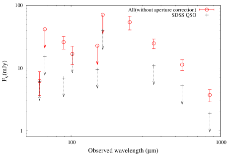
Figure 12: The 4-arcmin diameter aperture fluxes measured on $IRAS$, $AKARI$ and $Planck$ stacks of the HSC-SSP protoclusters and SDSS QSOs at $z\sim 4$. The red open circles show the average flux of a protocluster (all). The black crosses show the 2$\sigma$ upper limit fluxes of a SDSS QSO.

However, the average MIR luminosity, which is an excellent measure of AGN activity, of SDSS QSOs is not significantly different from that of the HzRGs of the known protoclusters; The IR SED of Spiderweb HzRG at $z=2.16$ is similar to that of the SDSS QSOs (Fig. 8). The HzRGs of the other known protoclusters at $z=2-3$ have $X$-ray luminosities $L_{2-10keV}=1\sim 4\times 10^{45}$ erg $s^{-1}$ (Pentericci et al., 2002; Scharf et al., 2003; Johnson et al., 2007; Macuga et al., 2019), which corresponds to $\nu L_{\nu}=10^{46}\sim 10^{47.5}$ erg $s^{-1}$ at $6~{}\mu$m ($\approx 0.03\sim 1$ mJy at $z=3.8$) according to the empirical $L_{2-10keV}$ v.s. $\nu L_{\nu}$ at a 6 $\mu$m relation (e.g., Stern 2015).

Meanwhile, the protoclusters at $z\sim 3.8$ show strong excess at $<100~{}\mu$m in the rest-frame which implies the overdensities and/or enhanced activities of obscured AGNs in the protoclusters correspond to $\sim$ ten times that of a SDSS QSO at $z\sim 4$ in the IR. Interestingly, warm/hot dust emission of the protoclusters becomes luminous approaching $z\sim 4$ while the change at $>100~{}\mu$m is small. Assuming that the excess warm/hot dust emission originates in AGNs, this implies that the growth of SMBHs in protoclusters peaks at $z\sim 4$ or more in advance of that in the general field at $z\sim 2$ (Madau & Dickinson, 2014). If this scenario is true, SDSS QSOs are not good landmarks of protoclusters at $z\sim 4$ because the proto-BCG like sources at $z\sim 4$ are more luminous than them but buried in dust formed by accompanying intense star formation.

6 Conclusion

By stacking Planck, AKARI, IRAS, WISE, and $H$-ATLAS images of the largest catalog of the protoclusters at $z\sim 4$ obtained by the HSC-SSP survey, we successfully show their average IR SED for the first time. The protoclusters at $z\sim 4$ are several tens of times brighter than a typical SFG at $z\sim 4$. They are on average as luminous as the most prominent protoclusters at $z=2-3$ and contain a larger warm/hot dust component. This suggests that protoclusters have rapidly evolved from $z=2$ to 4. The average IR SED of the protoclusters is unlike the average SED of a typical SFG but similar to IR luminous DOGs whose IR emission is dominated by AGNs. We evaluate the average SFR of the protoclusters by fitting the observed SEDs with SFG and AGN/SFG composite SED models. For the pure star-forming model, we find $L_{FIR}=19.3_{-4.2}^{+0.6}\times 10^{13}~{}L_{\odot}$ and SFR $=16.3_{-7.8}^{+1.0}\times 10^{3}~{}M_{\odot}$ yr^-1 while for the AGN/SFG composite model, we find $L_{FIR}=5.1_{-2.5}^{+2.5}\times 10^{13}~{}L_{\odot}$ and SFR$=2.1^{+6.3}_{-1.7}\times 10^{3}~{}M_{\odot}$ yr^-1. Their degeneracy cannot be solved via the SED fitting at this point; however, the contribution from AGNs is not empirically negligible. Our results are nearly consistent with previous CIB anisotropy studies, but at a shorter wavelength, CIB can be more biased in protocluster regions. Large uncertainty remained in the total SFR estimates; however, the total IR luminosity of the most massive clusters are likely to continue increasing up to $z\sim 4$. Stacking analysis of the QSOs at $z\sim 4$ optically selected is also performed and no excess star formation around them, as reported in Uchiyama et al. (2018), is confirmed.

Finally, we compare our results to the cosmological simulations of dusty SFGs to date (e.g., Chapman et al. 2009; Almeida et al. 2011; Hayward et al. 2013; Granato et al. 2015; Miller et al. 2015; Cowley et al. 2016; Lacey et al. 2016). Simulations predict that SMGs (e.g., with the flux over a few mJy in 850 $\mu$m in their definition) are in general strongly biased population hosted in massive halos with $M_{h}\hskip 3.00003pt\raisebox{1.72218pt}{$>$}\raisebox{-3.01385pt}{$\sim$}\hskip 3.00003pt10^{11.5}~{}M_{\odot}$ (Chapman et al., 2009; Almeida et al., 2011; Hayward et al., 2013; Miller et al., 2015; Cowley et al., 2016). Chapman et al. (2009) and Miller et al. (2015) predicted that the density excesses of SMGs do not always trace the most massive protoclusters. This agrees with our results that above 4$\sigma$ significance, the overdensity significance of $g$-dropout galaxies, which more tightly correlates with a halo mass, and the total IR luminosity do not correlate well. In addition, one or a few IR luminous DOGs such as in Fan et al. (2018) and Toba et al. (2018) can be responsible for the IR flux of a protocluster. If so, a protocluster may not be observed as an significant overdensity of SMGs. Simulations also predicted that the peak of the star formation history of cluster-sized halos is earlier than that in the general field (e.g., Chiang et al. 2017; Muldrew et al. 2018). Behroozi et al. (2013, 2019) linked the galaxy-halo assembly history from simulations and the observed galaxy properties, and found that halos with $M_{h}=10^{14}~{}M_{\odot}$ at present have a star formation history peak at $z\sim 3$. Our results suggests that the peak of the star formation history can be at $z>4$, earlier than that of the predictions using simulations and semi-observational methods.

Our results demonstrate the great importance of the IR properties of SFGs and AGNs in protoclusters “typical” at $z\sim 4$, for the first time. On the whole, our results suggest that DSFGs in protoclusters at $z\sim 4$ are more common than those predicted by current simulations. According to our results, simulations will need to approach the statistical behavior of the richest clusters with $M_{h}>10^{14}~{}M_{\odot}$ with a larger simulation box, dust emissivity at mid to far-IR, role of AGNs, and further constraints on the evolution of protoclusters at $z>3$ in the future. From the observational side, we can expand our study with HSC-SSP and next generation telescopes. Notably, the catalog used here is only a tenth of the whole HSC-SSP WIDE layer. In addition, Large Synoptic Survey Telescope will provide an additional large catalog of protoclusters in the future. These surveys will enable deeper stacking analysis for protoclusters at various redshifts. Characterization of individual IR sources in protoclusters is also needed though it is beyond the scope of this paper. Ito et al. (2019) optically selected the predominantly bright sources in some of our protocluster candidates as the candidate brightest cluster galaxies (BCGs). They are among the possible sources dominating the IR emission. Our study provides an excellent simulation for the James Webb Space Telescope (JWST) and Space Infrared Telescope for Cosmology and Astrophysics (SPICA). At this point, the deep observations with $8-10$ m class telescopes in the NIR, ALMA, $Chandra$, and $XMM-Newton$ telescopes are feasible to identify DSFGs/AGNs of protoclusters. However, given their large variation, several protoclusters at $z\sim 4$ need to be observed to evaluate a typical value.

Appendix A DATA SUMMARY

Table 6: Summary of the data

Instrument	Band	Wcena	FWHM PSFa	Point source detection limitb	1$\sigma$ (stack, 4’)c
		($\mu$m)	(arcmin)	(Jy)	(mJy)
Plancka	857 GHz	350	4.92	0.166	5.2
	545 GHz	540	4.68	0.118	2.8
	353 GHz	840	4.22	0.069	1.1
IRAS	60	60	3.6	0.6	4.7
	100	100	4.2	1.0	7.0

Note. — ^aThe central wavelengths and FWHM of the PSFs for $Planck$ are from https://wiki.cosmos.esa.int/planck-legacy-archive/index.php. For $IRAS$, $AKARI$, $WISE$ and $Herschel$, we refer $IRAS$ Explanatory Supplement (https://irsa.ipac.caltech.edu/IRASdocs/exp.sup), Doi et al. (2015) and Takita et al. (2015), http://wise2.ipac.caltech.edu/docs/release/allsky and https://www.cosmos.esa.int/web/herschel/home, respectively. For WISE, we list FWHM of the PSFs for Atlas image which are larger than those of a single exposure image. ^bThe point source detection limits in the literatures. For Planck, we refer the 90 % completeness limits listed in Table 1 of Planck collaboration XXXIX (2016), originally given in mJy. For IRAS, we refer the completeness limit for IRAS Point Source Catalog, Version 2.0 (Helou & Walker 1988; https://heasarc.gsfc.nasa.gov/W3Browse/iras /iraspsc.html). For AKARI, we refer AKARI/FIS All-Sky Survey Bright Source Catalogue Version 1.0 Release Note (https://www.ir.isas.jaxa.jp/AKARI/Archive/Catalogues/PSC/RN/AKARI-FIS_BSC_V1_RN.pdf). For Herschel, we refer the $5\sigma$ detection limit for H-ATLAS data release 1 (Valiante et al., 2016), originally given in mJy. For WISE, we refer the $5\sigma$ detection limit in the Release Note (http://wise2.ipac.caltech.edu/docs/release/allsky). ^cThe standard deviation of the fluxes in 4-arcmin diameters measured by 1000 times iteration of the stacking analysis at random positions in similar manner with the protoclusters ($N=216$ for Planck, IRAS, AKARI and WISE, and $N=93$ for $H$-ATLAS).

Table A1: Summary of the data –continues

Instrument	Band	Wcena	FWHM PSFa	Point source detection limitb	1$\sigma$ (stack, 4’)c
		($\mu$m)	(arcsec)	(Jy)	(mJy)
AKARI	N60	65	63.4	2.4	16
	WIDE-S	90	77.8	0.5	5.1
	WIDE-L	140	88.3	1.4	7.1
	N160	160	88.3d	6.3	14
Herschel	100	98	$11.8\times 11.0$	0.220	64
	160	154	$14.6\times 12.9$	0.245	48
	250	247	$18.4\times 17.4$	0.037	20
	350	347	$24.9\times 23.6$	0.047	6.5
	500	497	$37.0\times 33.8$	0.051	4.8
WISE	W1	3.368	8.25	0.068 $\times 10^{-3}$	0.56
	W2	4.618	8.25	0.098 $\times 10^{-3}$	0.27
	W3	12.082	8.25	0.86 $\times 10^{-3}$	0.16
	W4	22.194	16.5	5.4 $\times 10^{-3}$	0.27

Note. — ^dFWHM of the PSF for WIDE-L

Appendix B Stacking analysis simulation

We simulate the flux of a protocluster enclosed in an aperture by stacking mock images. Here four cases are assumed as follows: (1) one source at a random position within 2 arcmin, (2) three to five sources at random positions and flux values within 2.5 arcmin, (3) three to five sources at random positions and flux values within 5.0 arcmin from the center, and (4) observed distribution and fluxes of SMGs at $z_{\rm spec}\approx 3.09$ in the SSA22 protocluster. Their average flux distributions are more extended in the order of (1)$<$(2)$<$(4)$<$(3). At total of 214 mock images are generated and, smooth the images to have FWHM PSF 4.9 arcmin;, and they are stacked for each case. The total flux of the sources on a mock image is a fixed value. In case (4), random rotations and random shifts within 2 arcmin centering at the brightest source are added.

Fig. 1 shows the simulated images. We compare the observed radial profiles of the protoclusters at 857 GHz smoothed to have a FWHM of the PSF 4.9 arcmin to the simulations in Fig. 2 (left). The observed radial profiles are more extended than that of a point source. All protoclusters are similar to case (1) and (2) while the brighter-half protoclusters are more similar to case (4). Fig. 2 (right) shows the flux fraction enclosed in an aperture. In cases (1), (2) and (4), $\sim 29\%,~{}28\%$, and $22$ % of the total fluxes are enclosed in a 2 arcmin aperture radius. The aperture correction factors obtained using Herschel as in Section 3.4 are identical to them.

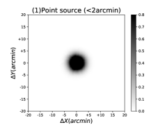
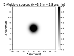
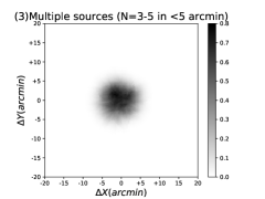
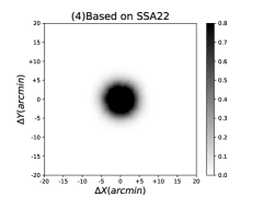
Figure 1: Simulation of the stacking analysis in case (1) to (4) from left to right

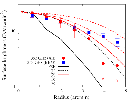
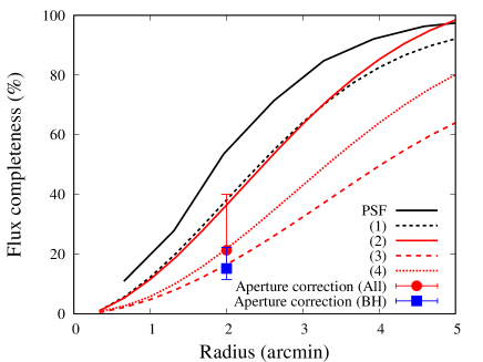
Figure 2: Left: Radial profiles of the protoclusters compared with the simulations. The black solid curve shows the radial profile of a point source. The black dashed curve, and red solid, dashed, and dotted curves show the average radial profiles for case (1), (2), (3), and (4) measured by a thousand times iterations for each. The red filled circles and blue filled squares show the radial profiles of the all and brighter-half protoclusters measured on the stacked images at Planck 857 GHz smoothed to have FWHM of the PSF 4.9 arcmin. Right: Similar to left panel but flux completenesses at a given aperture are shown in $y$-axis. The red filled circle and blue filled square show the aperture correction factors found in Section 3.4.

Appendix C Fainter half protoclusters

Figures 2 and 2 show the $Planck$ 353, 545, and 857-GHz stacks for the 1st quartile and 2nd quertile from the lowest of the 857 GHz flux distribution of the protoclusters (Fig. 2).

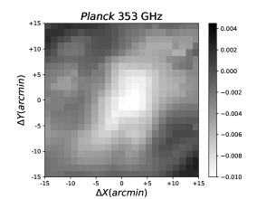
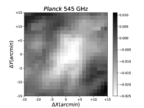
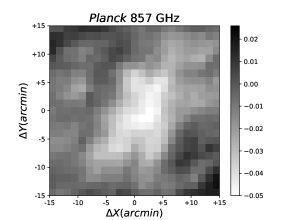
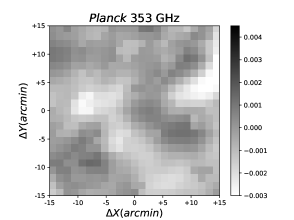
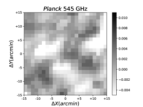
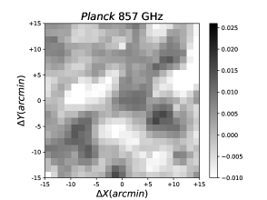
Figure 1: $Planck$ 353, 545, and 857-GHz stacks for the 1st quartile from the lowest of the flux distribution of the protoclusters, from left to right.

Figure 2: $Planck$ 353, 545, and 857-GHz stacks for the 2nd quartile from the lowest of the flux distribution of the protoclusters, from left to right.

References

- Alberts et al. (2016) Alberts, S., Pope, A., Brodwin, M., et al. 2016, ApJ, 825, 72.
- Almeida et al. (2011) Almeida, C., Baugh, C. M., & Lacey, C. G. 2011, MNRAS, 417, 2057
- Álvarez-Márquez et al. (2019) Álvarez-Márquez, J., Burgarella, D., Buat, V., et al. 2019, A&A, 630, A153
- Amblard et al. (2011) Amblard, A., Cooray, A., Serra, P., et al. 2011, Nature, 470, 510
- Arrigoni Battaia et al. (2018) Arrigoni Battaia, F., Chen, C.-C., Fumagalli, M., et al. 2018, A&A, 620, A202
- Aihara et al. (2018) Aihara, H., Arimoto, N., Armstrong, R., et al. 2018, PASJ, 70, S4
- Behroozi et al. (2013) Behroozi, P. S., Wechsler, R. H., & Conroy, C. 2013, ApJ, 770, 57
- Behroozi et al. (2019) Behroozi, P., Wechsler, R. H., Hearin, A. P., et al. 2019, MNRAS, 488, 3143
- Bell (2003) Bell, E. F. 2003, ApJ, 586, 794
- Bertin & Arnouts (1996) Bertin, E., & Arnouts, S. 1996, A&AS, 117, 393
- Béthermin et al. (2012) Béthermin, M., Le Floc’h, E., Ilbert, O., et al. 2012, A&A, 542, A58
- Béthermin et al. (2013) Béthermin, M., Wang, L., Doré, O., et al. 2013, A&A, 557, A66
- Béthermin et al. (2015) Béthermin, M., Daddi, E., Magdis, G., et al. 2015, A&A, 573, A113
- Blain et al. (2004) Blain, A. W., Chapman, S. C., Smail, I., et al. 2004, ApJ, 611, 725
- Bourne et al. (2017) Bourne, N., Dunlop, J. S., Merlin, E., et al. 2017, MNRAS, 467, 1360
- Bouwens et al. (2016) Bouwens, R. J., Aravena, M., Decarli, R., et al. 2016, ApJ, 833, 72
- Braglia et al. (2011) Braglia, F. G., Ade, P. A. R., Bock, J. J., et al. 2011, MNRAS, 412, 1187
- Bruzual & Charlot (2003) Bruzual, G., & Charlot, S. 2003, MNRAS, 344, 1000
- Casey et al. (2014) Casey, C. M., Narayanan, D., & Cooray, A. 2014, Phys. Rep., 541, 45
- Casey et al. (2015) Casey, C. M., Cooray, A., Capak, P., et al. 2015, ApJ, 808, L33
- Casey (2016) Casey, C. M. 2016, ApJ, 824, 36
- Chabrier (2003) Chabrier, G. 2003, ApJ, 586, L133
- Chapman et al. (2009) Chapman, S. C., Blain, A., Ibata, R., et al. 2009, ApJ, 691, 560
- Charlot & Fall (2000) Charlot, S., & Fall, S. M. 2000, ApJ, 539, 718
- Chiang et al. (2013) Chiang, Y.-K., Overzier, R., & Gebhardt, K. 2013, ApJ, 779, 127
- Chiang et al. (2017) Chiang, Y.-K., Overzier, R. A., Gebhardt, K., et al. 2017, ApJ, 844, L23
- Chung et al. (2010) Chung, S. M., Gonzalez, A. H., Clowe, D., et al. 2010, ApJ, 725, 1536
- Clements et al. (2014) Clements, D. L., Braglia, F. G., Hyde, A. K., et al. 2014, MNRAS, 439, 1193
- Clements et al. (2016) Clements, D. L., Braglia, F., Petitpas, G., et al. 2016, MNRAS, 461, 1719
- Cowley et al. (2016) Cowley, W. I., Lacey, C. G., Baugh, C. M., et al. 2016, MNRAS, 461, 1621
- da Cunha et al. (2008) da Cunha, E., Charlot, S., & Elbaz, D. 2008, MNRAS, 388, 1595
- Dannerbauer et al. (2014) Dannerbauer, H., Kurk, J. D., De Breuck, C., et al. 2014, A&A, 570, A55
- De Lucia & Blaizot (2007) De Lucia, G., & Blaizot, J. 2007, MNRAS, 375, 2
- Digby-North et al. (2010) Digby-North, J. A., Nandra, K., Laird, E. S., et al. 2010, MNRAS, 407, 846
- Doi et al. (2015) Doi, Y., Takita, S., Ootsubo, T., et al. 2015, PASJ, 67, 50
- Dole et al. (2006) Dole, H., Lagache, G., Puget, J.-L., et al. 2006, A&A, 451, 417
- Fadda et al. (2000) Fadda, D., Elbaz, D., Duc, P.-A., et al. 2000, A&A, 361, 827
- Faisst et al. (2017) Faisst, A. L., Capak, P. L., Yan, L., et al. 2017, ApJ, 847, 21
- Fan et al. (2018) Fan, L., Gao, Y., Knudsen, K. K., & Shu, X. 2018, ApJ, 854, 157
- Galametz et al. (2012) Galametz, A., Stern, D., De Breuck, C., et al. 2012, ApJ, 749, 169
- Geach et al. (2006) Geach, J. E., Smail, I., Ellis, R. S., et al. 2006, ApJ, 649, 661
- Gómez-Guijarro et al. (2019) Gómez-Guijarro, C., Riechers, D. A., Pavesi, R., et al. 2019, ApJ, 872, 117
- Goto et al. (2017) Goto, T., Utsumi, Y., Kikuta, S., et al. 2017, MNRAS, 470, L117
- Granato et al. (2015) Granato, G. L., Ragone-Figueroa, C., Domínguez-Tenreiro, R., et al. 2015, MNRAS, 450, 1320
- Greenslade et al. (2018) Greenslade, J., Clements, D. L., Cheng, T., et al. 2018, MNRAS, 476, 3336.
- Gruppioni et al. (2013) Gruppioni, C., Pozzi, F., Rodighiero, G., et al. 2013, MNRAS, 432, 23
- Haines et al. (2009) Haines, C. P., Smith, G. P., Egami, E., et al. 2009, MNRAS, 396, 1297
- Harikane et al. (2019) Harikane, Y., Ouchi, M., Ono, Y., et al. 2019, arXiv e-prints , arXiv:1902.09555.
- Hatch et al. (2014) Hatch, N. A., Wylezalek, D., Kurk, J. D., et al. 2014, MNRAS, 445, 280
- Hayashino et al. (2004) Hayashino, T., Matsuda, Y., Tamura, H., et al. 2004, AJ, 128, 2073
- Hayward et al. (2013) Hayward, C. C., Narayanan, D., Kereš, D., et al. 2013, MNRAS, 428, 2529
- Helou & Walker (1988) Helou, G., & Walker, D. W. 1988, Infrared astronomical satellite (IRAS) catalogs and atlases. Volume 7, p.1-265, 7, 1
- Hickox & Alexander (2018) Hickox, R. C., & Alexander, D. M. 2018, arXiv:1806.04680
- Higuchi et al. (2019) Higuchi, R., Ouchi, M., Ono, Y., et al. 2019, ApJ, 879, 28
- Ishigaki et al. (2016) Ishigaki, M., Ouchi, M., & Harikane, Y. 2016, ApJ, 822, 5
- Ito et al. (2019) Ito, K., Kashikawa, N., Toshikawa, J., et al. 2019, ApJ, 878, 68
- Johnson et al. (2007) Johnson, O., Almaini, O., Best, P. N., & Dunlop, J. 2007, MNRAS, 376, 151
- Kashikawa et al. (2007) Kashikawa, N., Kitayama, T., Doi, M., et al. 2007, ApJ, 663, 765
- Kato et al. (2016) Kato, Y., Matsuda, Y., Smail, I., et al. 2016, MNRAS, 460, 3861
- Kawada et al. (2007) Kawada, M., Baba, H., Barthel, P. D., et al. 2007, PASJ, 59, S389
- Kennicutt (1998) Kennicutt, R. C. 1998, ARA&A, 36, 189
- Kikuta et al. (2017) Kikuta, S., Imanishi, M., Matsuoka, Y., et al. 2017, ApJ, 841, 128
- Kikuta et al. (2019) Kikuta, S., Matsuda, Y., Cen, R., et al. 2019, PASJ, 71, L2
- Kim et al. (2009) Kim, S., Stiavelli, M., Trenti, M., et al. 2009, ApJ, 695, 809
- Kodama et al. (2007) Kodama, T., Tanaka, I., Kajisawa, M., et al. 2007, MNRAS, 377, 1717
- Koprowski et al. (2018) Koprowski, M. P., Coppin, K. E. K., Geach, J. E., et al. 2018, MNRAS, 479, 4355
- Koyama et al. (2013) Koyama, Y., Kodama, T., Tadaki, K.-. ichi ., et al. 2013, MNRAS, 428, 1551
- Krishnan et al. (2017) Krishnan, C., Hatch, N. A., Almaini, O., et al. 2017, MNRAS, 470, 2170.
- Kubo et al. (2013) Kubo, M., Uchimoto, Y. K., Yamada, T., et al. 2013, ApJ, 778, 170
- Kubo et al. (2015) Kubo, M., Yamada, T., Ichikawa, T., et al. 2015, ApJ, 799, 38
- Kubo et al. (2016) Kubo, M., Yamada, T., Ichikawa, T., et al. 2016, MNRAS, 455, 3333
- Kurk et al. (2000) Kurk, J. D., Röttgering, H. J. A., Pentericci, L., et al. 2000, A&A, 358, L1
- Kurk et al. (2004) Kurk, J. D., Pentericci, L., Röttgering, H. J. A., et al. 2004, A&A, 428, 793
- Lacey et al. (2016) Lacey, C. G., Baugh, C. M., Frenk, C. S., et al. 2016, MNRAS, 462, 3854
- Lagache et al. (2005) Lagache, G., Puget, J.-L., & Dole, H. 2005, ARA&A, 43, 727
- Lehmer et al. (2009) Lehmer, B. D., Alexander, D. M., Geach, J. E., et al. 2009, ApJ, 691, 687
- Lehmer et al. (2013) Lehmer, B. D., Lucy, A. B., Alexander, D. M., et al. 2013, ApJ, 765, 87
- Liang et al. (2019) Liang, L., Feldmann, R., Kereš, D., et al. 2019, MNRAS, 489, 1397
- Macuga et al. (2019) Macuga, M., Martini, P., Miller, E. D., et al. 2019, ApJ, 874, 54
- Madau (1995) Madau, P. 1995, ApJ, 441, 18
- Madau & Dickinson (2014) Madau, P., & Dickinson, M. 2014, ARA&A, 52, 415
- Magdis et al. (2012) Magdis, G. E., Daddi, E., Béthermin, M., et al. 2012, ApJ, 760, 6
- Maniyar et al. (2018) Maniyar, A. S., Béthermin, M., & Lagache, G. 2018, A&A, 614, A39
- Matsuda et al. (2004) Matsuda, Y., Yamada, T., Hayashino, T., et al. 2004, AJ, 128, 569
- Matsuda et al. (2011) Matsuda, Y., Smail, I., Geach, J. E., et al. 2011, MNRAS, 416, 2041
- Meusinger et al. (2000) Meusinger, H., Brunzendorf, J., & Krieg, R. 2000, A&A, 363, 933
- Miller et al. (2015) Miller, T. B., Hayward, C. C., Chapman, S. C., et al. 2015, MNRAS, 452, 878
- Miller et al. (2018) Miller, T. B., Chapman, S. C., Aravena, M., et al. 2018, Nature, 556, 469
- Miyazaki et al. (2012) Miyazaki, S., Komiyama, Y., Nakaya, H., et al. 2012, Proc. SPIE, 8446, 84460Z
- Muldrew et al. (2018) Muldrew, S. I., Hatch, N. A., & Cooke, E. A. 2018, MNRAS, 473, 2335
- Murakami et al. (2007) Murakami, H., Baba, H., Barthel, P., et al. 2007, PASJ, 59, S369
- Neugebauer et al. (1984) Neugebauer, G., Habing, H. J., van Duinen, R., et al. 1984, ApJ, 278, L1
- Noirot et al. (2016) Noirot, G., Vernet, J., De Breuck, C., et al. 2016, ApJ, 830, 90
- Noirot et al. (2018) Noirot, G., Stern, D., Mei, S., et al. 2018, ApJ, 859, 38
- Onoue et al. (2018) Onoue, M., Kashikawa, N., Uchiyama, H., et al. 2018, PASJ, 70, S31
- Ota et al. (2018) Ota, K., Venemans, B. P., Taniguchi, Y., et al. 2018, ApJ, 856, 109
- Oteo et al. (2018) Oteo, I., Ivison, R. J., Dunne, L., et al. 2018, ApJ, 856, 72
- Pentericci et al. (2002) Pentericci, L., Kurk, J. D., Carilli, C. L., et al. 2002, A&A, 396, 109
- Planck collaboration I (2011) Planck Collaboration, Ade, P. A. R., Aghanim, N., et al. 2011, A&A, 536, A1
- Planck collaboration XVIII (2011) Planck Collaboration, Ade, P. A. R., Aghanim, N., et al. 2011, A&A, 536, A18
- Planck collaboration VI (2014) Planck Collaboration 2013 IV, Ade, P. A. R., Aghanim, N., et al. 2014, A&A, 571, A6
- Planck collaboration XXX (2014) Planck Collaboration, Ade, P. A. R., Aghanim, N., et al. 2014, A&A, 571, A30
- Planck collaboration XXXIX (2016) Planck Collaboration 2016, Ade, P. A. R., Aghanim, N., et al. 2016, A&A, 596, A100
- Planck collaboration XLVIII (2016) Planck Collaboration 2016 XLVIII, Aghanim, N., Ashdown, M., et al. 2016, A&A, 596, A109
- Polletta et al. (2006) Polletta, M. d. C., Wilkes, B. J., Siana, B., et al. 2006, ApJ, 642, 673
- Scharf et al. (2003) Scharf, C., Smail, I., Ivison, R., et al. 2003, ApJ, 596, 105
- Schmidt et al. (2015) Schmidt, S. J., Ménard, B., Scranton, R., et al. 2015, MNRAS, 446, 2696
- Shi et al. (2019) Shi, K., Lee, K.-S., Dey, A., et al. 2019, ApJ, 871, 83
- Shimakawa et al. (2018) Shimakawa, R., Koyama, Y., Röttgering, H. J. A., et al. 2018, MNRAS, 481, 5630
- Siebenmorgen et al. (2015) Siebenmorgen, R., Heymann, F., & Efstathiou, A. 2015, A&A, 583, A120
- Smith et al. (2019) Smith, C. M. A., Gear, W. K., Smith, M. W. L., et al. 2019, MNRAS, 486, 4304.
- Spitler et al. (2012) Spitler, L. R., Labbé, I., Glazebrook, K., et al. 2012, ApJ, 748, L21
- Steidel et al. (1998) Steidel, C. C., Adelberger, K. L., Dickinson, M., et al. 1998, ApJ, 492, 428
- Steidel et al. (2000) Steidel, C. C., Adelberger, K. L., Shapley, A. E., et al. 2000, ApJ, 532, 170
- Stevens et al. (2010) Stevens, J. A., Jarvis, M. J., Coppin, K. E. K., et al. 2010, MNRAS, 405, 2623
- Stern (2015) Stern, D. 2015, ApJ, 807, 129
- Takita et al. (2015) Takita, S., Doi, Y., Ootsubo, T., et al. 2015, PASJ, 67, 51
- Tamura et al. (2009) Tamura, Y., Kohno, K., Nakanishi, K., et al. 2009, Nature, 459, 61
- Tanaka et al. (2011) Tanaka, I., De Breuck, C., Kurk, J. D., et al. 2011, PASJ, 63, 415
- Toba et al. (2018) Toba, Y., Ueda, J., Lim, C.-F., et al. 2018, ApJ, 857, 31
- Toshikawa et al. (2012) Toshikawa, J., Kashikawa, N., Ota, K., et al. 2012, ApJ, 750, 137
- Toshikawa et al. (2016) Toshikawa, J., Kashikawa, N., Overzier, R., et al. 2016, ApJ, 826, 114
- Toshikawa et al. (2018) Toshikawa, J., Uchiyama, H., Kashikawa, N., et al. 2018, PASJ, 70, S12
- Uchimoto et al. (2012) Uchimoto, Y. K., Yamada, T., Kajisawa, M., et al. 2012, ApJ, 750, 116
- Uchiyama et al. (2018) Uchiyama, H., Toshikawa, J., Kashikawa, N., et al. 2018, PASJ, 70, S32
- Umehata et al. (2014) Umehata, H., Tamura, Y., Kohno, K., et al. 2014, MNRAS, 440, 3462
- Umehata et al. (2017) Umehata, H., Tamura, Y., Kohno, K., et al. 2017, ApJ, 835, 98
- Umehata et al. (2018) Umehata, H., Hatsukade, B., Smail, I., et al. 2018, PASJ, 70, 65
- Valiante et al. (2016) Valiante, E., Smith, M. W. L., Eales, S., et al. 2016, MNRAS, 462, 3146
- Venemans et al. (2007) Venemans, B. P., Röttgering, H. J. A., Miley, G. K., et al. 2007, A&A, 461, 823
- Viero et al. (2013) Viero, M. P., Moncelsi, L., Quadri, R. F., et al. 2013, ApJ, 779, 32
- Wang et al. (2016) Wang, T., Elbaz, D., Daddi, E., et al. 2016, ApJ, 828, 56
- Webb et al. (2009) Webb, T. M. A., Yamada, T., Huang, J.-S., et al. 2009, ApJ, 692, 1561
- Wright et al. (2010) Wright, E. L., Eisenhardt, P. R. M., Mainzer, A. K., et al. 2010, AJ, 140, 1868
- Wylezalek et al. (2013) Wylezalek, D., Galametz, A., Stern, D., et al. 2013, ApJ, 769, 79
- Wylezalek et al. (2014) Wylezalek, D., Vernet, J., De Breuck, C., et al. 2014, ApJ, 786, 17
- Yuan et al. (2014) Yuan, T., Nanayakkara, T., Kacprzak, G. G., et al. 2014, ApJ, 795, L20