Photon pair production in gluon fusion: Top quark effects at NLO with threshold matching

Abstract

We present a calculation of the NLO QCD corrections to the loop-induced production of a photon pair through gluon fusion, including massive top quarks at two loops, where the two-loop integrals are calculated numerically. Matching the fixed-order NLO results to a threshold expansion, we obtain accurate results around the top quark pair production threshold. We analyse how the top quark threshold corrections affect distributions of the photon pair invariant mass and comment on the possibility of determining the top quark mass from precision measurements of the diphoton invariant mass spectrum.

1 Introduction

The production of pairs of photons in hadronic collisions has attracted interest from both the experimental and the theory side for several decades. Most prominently, the diphoton final state served as one of the key discovery channels for the Higgs boson Chatrchyan:2014fsa ; Aaboud:2017vol , which can decay into two photons. As a very clean experimental channel, it is also well suited for precision studies of the Standard Model (SM) and in particular the Higgs sector. For example, there is the possibility to constrain the Higgs boson width from interference effects of the continuum $gg\to\gamma\gamma$ spectrum with the signal $gg\to H\to\gamma\gamma$ Dicus:1987fk ; Dixon:2003yb ; Martin:2012xc ; deFlorian:2013psa ; Martin:2013ula ; Dixon:2013haa ; Campbell:2017rke ; Cieri:2017kpq . Furthermore, various New Physics models predict the production of photon pairs, where the study of angular correlations between the decay photons can provide information about the spin of the underlying resonances Aaboud:2016tru ; Sirunyan:2018wnk .

Another interesting aspect of diphoton production is the possibility of measuring the top quark mass via the top quark pair production threshold effects manifest in the diphoton invariant mass spectrum Jain:2016kai ; Kawabata:2016aya . While current LHC measurements Aaboud:2017vol ; Chatrchyan:2014fsa are not yet able to provide the necessary statistics for such a threshold scan, the feasibility at the High-Luminosity LHC, and even more so at a future 100 TeV collider, is worth investigating.

Direct diphoton production in hadronic collisions occurs via the leading order (LO) $\alpha_{s}^{0}$ process $q\bar{q}\to\gamma\gamma$. The next-to-leading order (NLO) QCD corrections to this process, including fragmentation contributions at NLO, were implemented in the public program Diphox Binoth:1999qq .

The loop induced $gg\to\gamma\gamma$ process enters as a next-to-next-to-leading order (NNLO) QCD (order $\alpha_{s}^{2}$) correction to the $pp\to\gamma\gamma$ cross section. The process $gg\to\gamma\gamma$ has been calculated at LO including both massless and massive quark loops in Ref. Dicus:1987fk and is included in Diphox at one loop for massless quark loops. Even though the $gg\to\gamma\gamma$ contribution is a higher-order correction to the total $pp\to\gamma\gamma$ cross section, its contribution is similar in size to the LO result at the LHC, due to the large gluon luminosity. A calculation that includes also the effects of transverse-momentum resummation to direct photon production is implemented in the program ResBos Balazs:2007hr .

NLO QCD corrections to the gluon-fusion channel with massless quarks, i.e. ${\cal O}(\alpha_{s}^{3})$ corrections, have been first calculated in Refs. Bern:2001df ; Bern:2002jx and implemented in the code 2$\gamma$MC Bern:2002jx as well as in MCFM Campbell:2011bn . Very recently, the NLO QCD corrections to the gluon-fusion channel including massive top quark loops have become available Maltoni:2018zvp , where the master integrals have been calculated numerically based on the numerical solution of differential equations Czakon:2008zk ; Mandal:2018cdj . Analytic results for the planar two-loop box integrals with massive top quarks have been presented in Ref. Caron-Huot:2014lda ; Becchetti:2017abb . Regarding the non-planar contributions, 3-point topologies containing elliptic integrals have been calculated in Ref. vonManteuffel:2017hms ; Broedel:2019hyg . Other 3-point topologies have been calculated earlier in the context of Higgs production and decay Aglietti:2006tp ; Anastasiou:2006hc .

The NNLO QCD corrections to the process $pp\to\gamma\gamma$ were first calculated in Ref. Catani:2011qz , including the $gg\to\gamma\gamma$ contribution at order $\alpha_{s}^{2}$ with massless quark loops. For a phenomenological study see also Ref. Catani:2018krb . The NNLO QCD corrections to $pp\to\gamma\gamma$ have also been calculated and implemented in MCFM in Ref. Campbell:2016yrh , supplemented by the $gg$ initiated loops proportional to $n_{f}$ at LO and NLO for five massless quark flavours, and at LO for massive top quark loops. Diphoton production at NNLO with massless quarks is also available in Matrix Grazzini:2017mhc .

The aim of this paper is twofold. Firstly, we provide an independent calculation of the QCD corrections to the process $gg\to\gamma\gamma$ including massive top quark loops, confirming the results of Ref. Maltoni:2018zvp for the central scale choice. Secondly, we combine our results with threshold resummation as advocated in Ref. Kawabata:2016aya , such that the top quark pair production threshold region in the diphoton invariant mass spectrum can be predicted with high accuracy. The calculation can thus serve as a starting point for investigating the possibility of a top quark mass measurement from the diphoton invariant mass spectrum.

This work is structured as follows. In Section 2 we describe our calculation of the NLO corrections including both massless and massive fermion loops. Section 3 contains a description of our treatment of the top quark pair production threshold region. In Section 4 we present our numerical results. Finally, in Section 5 we summarise and present an outlook on the possibility of measuring the top quark mass from the diphoton spectrum.

2 Building blocks of the fixed order calculation

We consider the following scattering process,

$$g(p_{1},\lambda_{1},a_{1})+g(p_{2},\lambda_{2},a_{2})\to\gamma(p_{3},\lambda_{3})+\gamma(p_{4},\lambda_{4}),$$ (1)

with on-shell conditions $p_{j}^{2}=0,j=1,...,4$. The helicities $\lambda_{i}$ of the external particles are defined by taking the momenta of the gluons $p_{1}$ and $p_{2}$ (with colour indices $a_{1}$ and $a_{2}$, respectively) as incoming and the momenta of the photons $p_{3}$ and $p_{4}$ as outgoing. The Mandelstam invariants associated with eq. (1) are defined by

$$s=\left(p_{1}+p_{2}\right)^{2}, t=\left(p_{2}-p_{3}\right)^{2}, u=\left(p_{1}-p_{3}\right)^{2}.$$ (2)

2.1 Calculation of the virtual amplitudes

Projection operators

We define the tensor amplitude $\mathcal{M}_{\mu_{1}\mu_{2}\mu_{3}\mu_{4}}$ by extracting the polarisation vectors from the amplitude $\mathcal{M}$,

$$\mathcal{M}{}=\varepsilon_{\lambda_{1}}^{\mu_{1}}(p_{1})\,\varepsilon_{\lambda_{2}}^{\mu_{2}}(p_{2})\,\varepsilon_{\lambda_{3}}^{\mu_{3},\star}(p_{3})\,\varepsilon_{\lambda_{4}}^{\mu_{4},\star}(p_{4})\,\mathcal{M}_{\mu_{1}\mu_{2}\mu_{3}\mu_{4}}(p_{1},p_{2},p_{3},p_{4}),$$ (3)

where the $\varepsilon_{\lambda_{i}}^{\mu_{i}}$ denote the polarisation vectors. The amplitude is computed through projection onto a set of Lorentz structures related to linear polarisation states of the external massless bosons. An appropriate set of $D$-dimensional projection operators is constructed following the approach proposed in Ref. Chen:2019wyb , which has been applied recently in the calculation of Ref. Ahmed:2019udm , and which we will summarise briefly in the following.

A physical polarisation vector $\varepsilon(p)$ of a massless vector boson with (on-shell) momentum $p$ fulfils the transversality and (imposed) normalisation conditions,

$$\varepsilon(p)\cdot p=0,\quad\varepsilon(p)\cdot\varepsilon(p)=-1.$$ (4)

These conditions fix two components of the polarisation vectors in four space-time dimensions. Now we construct explicitly a basis of the space of polarisation states defined by (4) for the external massless vector bosons. First, we introduce a polarisation basis vector $\varepsilon_{X}$, valid for both intial-state gluons, which can be written in terms of the linearly independent momenta of the process

$$\varepsilon_{X}^{\mu}=c_{1}^{X}\,p_{1}^{\mu}+c_{2}^{X}\,p_{2}^{\mu}+c_{3}^{X}\,p_{3}^{\mu}\;,$$ (5)

where the Lorentz invariant coefficients $c_{i}^{X}$ are determined by the system of equations

$$\varepsilon_{X}\cdot p_{1}=0,\qquad\varepsilon_{X}\cdot p_{2}=0,\qquad\varepsilon_{X}\cdot\varepsilon_{X}=-1.$$ (6)

Note that the conditions above constitute a gauge choice in which the reference momentum of either incoming gluon is set to be the momentum of the other gluon. A polarisation vector $\varepsilon_{T}$ for both outgoing photons can be constructed analogously:

$$\varepsilon_{T}\cdot p_{3}=0,\qquad\varepsilon_{T}\cdot p_{4}=0,\qquad\varepsilon_{T}\cdot\varepsilon_{T}=-1.$$ (7)

A third basis vector $\varepsilon_{Y}$, pointing out of the scattering plane, is needed to span the space of all possible polarisation vectors for this process:

$$\varepsilon_{Y}\cdot p_{i}=0,\qquad i\in\{1,\ldots,4\}\;.$$ (8)

In four dimensions, such a vector can be constructed using the Levi-Civita tensor:

$$\varepsilon_{Y}^{\mu}=\varepsilon^{\mu\nu\rho\sigma}{p_{1}}_{\nu}\,{p_{2}}_{\rho}\,{p_{3}}_{\sigma}.$$ (9)

Since we consider only QCD corrections to a QED process, neither $\gamma{}_{5}$ nor Levi-Civita tensors are introduced by the relevant Feynman rules. Consequently, a completely $D$-dimensional tensor decomposition of this scattering amplitude can be expressed solely in terms of metric tensors and external momenta. Therefore, a contraction of the tensor amplitude with an odd number of $\varepsilon_{Y}$ evaluates to zero. A product of two Levi-Civita tensors, however, can be rewritten in terms of metric tensors using

$$\varepsilon^{\mu\nu\rho\sigma}\,\varepsilon{}_{\alpha\beta\kappa\lambda}=\det\left(\begin{array}[]{cccc}\delta_{\alpha}^{\mu}&\delta_{\beta}^{\mu}&\delta_{\kappa}^{\mu}&\delta_{\lambda}^{\mu}\\ \delta_{\alpha}^{\nu}&\delta_{\beta}^{\nu}&\delta_{\kappa}^{\nu}&\delta_{\lambda}^{\nu}\\ \delta_{\alpha}^{\rho}&\delta_{\beta}^{\rho}&\delta_{\kappa}^{\rho}&\delta_{\lambda}^{\rho}\\ \delta_{\alpha}^{\sigma}&\delta_{\beta}^{\sigma}&\delta_{\kappa}^{\sigma}&\delta_{\lambda}^{\sigma}\end{array}\right),$$ (10)

which has a straightforward $D$-dimensional continuation. For a detailed discussion of the subtleties related to the manipulation of Levi-Civita tensors in the construction of projectors for more general cases we refer to Ref. Chen:2019wyb .  

Applied to the scattering process (1), this construction leads to eight projectors

$$\varepsilon_{[X,Y]}^{\mu}\varepsilon_{[X,Y]}^{\nu}\varepsilon_{[T,Y]}^{\rho}\varepsilon_{[T,Y]}^{\sigma},$$ (11)

where the square bracket $[\cdot{},\cdot{}]$ means either entry and where only the combinations containing an even number of $\varepsilon_{Y}$ are considered. Let us emphasize again that, in order to avoid possible ambiguities in the application of these projectors, all pairs of Levi-Civita tensors are replaced according to the contraction rule (10) before being used for the projection of the amplitude. Then the aforementioned projectors are expressed solely in terms of external momenta and metric tensors whose open Lorentz indices are all set to be $D$-dimensional.

The usual helicity amplitudes can be constructed as circular polarisation states from the linear ones using the relations

$$\begin{split}\varepsilon_{\pm}(p_{1})^{\mu}&=\frac{1}{\sqrt{2}}\left(\varepsilon_{X}^{\mu}\pm i\varepsilon_{Y}^{\mu}\right),\\ \varepsilon_{\pm}(p_{2})^{\nu}&=\frac{1}{\sqrt{2}}\left(\varepsilon_{X}^{\nu}\mp i\varepsilon_{Y}^{\nu}\right),\\ \varepsilon_{\pm}(p_{3})^{\rho}&=\frac{1}{\sqrt{2}}\left(\varepsilon_{T}^{\rho}\pm i\varepsilon_{Y}^{\rho}\right),\\ \varepsilon_{\pm}(p_{4})^{\sigma}&=\frac{1}{\sqrt{2}}\left(\varepsilon_{T}^{\sigma}\mp i\varepsilon_{Y}^{\sigma}\right).\end{split}$$ (12)

Analytic results for the LO amplitudes of (1) were obtained quite some time ago in Refs. Karplus:1950zz ; Bern:2001dg ; Binoth:2002xg for massless quark loop contributions and in Refs. Bern:1995db ; Bernicot:2008th with massive quark loop contributions. With the linear polarisation projectors defined in (11), we re-computed these LO amplitudes analytically, with both massless and massive quark loops. These expressions were implemented in our computational setup for the NLO QCD corrections to the considered process, which we describe below.

UV renormalisation

The bare scattering amplitudes of the process (1), denoted by $\hat{\mathcal{M}}$, beyond LO contain poles in the dimensional regulator $\epsilon\equiv(4-D)/2$ arising from ultraviolet (UV) as well as soft and collinear (IR) regions of the loop momenta. In our computation, we renormalise these UV divergences using the $\overline{\text{MS}}$ scheme, except for the top quark mass which is renormalised on-shell.

The bare virtual amplitude $\hat{\mathcal{M}}$ is a function of the bare QCD coupling $\hat{\alpha}_{s}$ and the bare top quark mass $\hat{m}_{t}$. The UV renormalisation of $\hat{\mathcal{M}}$ is achieved by the replacement

$$\hat{\alpha}_{s}\,\hat{\mu}^{2\epsilon}\,S_{\epsilon}=\alpha_{s}\,\mu_{R}^{2\epsilon}\,Z_{a}\;,\;\hat{m}_{t}=m_{t}\,Z_{m},$$ (13)

and by renormalising the gluon wave function. Here, $S_{\epsilon}=\left(4\pi\right)^{\epsilon}e^{-\epsilon\gamma_{E}}$, with $\gamma_{E}$ the Euler constant. The strong coupling is given by $\alpha_{s}=g_{s}^{2}/(4\pi)$ and $\hat{\mu}$ is an auxiliary mass-dimensionful parameter introduced in dimensional regularisation to keep the coupling constants dimensionless. The usual renormalisation scale is denoted $\mu_{R}$, and we will use $\hat{\mu}=\mu_{R}$ in the following.

Both the bare virtual amplitudes and the UV renormalisation constants are expanded in $a_{s}\equiv\alpha_{s}(\mu_{R})/(4\pi)$. We may write the renormalisation constants as

$$Z_{i}=1+a_{s}\,\delta Z_{i}+O(a_{s}^{2}),\qquad i=a,A,m.$$ (14)

Under the $\overline{\text{MS}}$ scheme for $\alpha_{s}$ with $n_{f}$ massless quark flavours and top-quark loops renormalised on-shell, the renormalisation constants needed in our computation read

$$\delta Z_{a} =-\frac{1}{\epsilon}\,\beta_{0}+\left(\frac{\mu_{R}^{2}}{m_{t}^{2}}\right)^{\epsilon}\frac{4}{3\epsilon}\,T_{R},$$

$$\delta Z_{A} =\left(\frac{\mu_{R}^{2}}{m_{t}^{2}}\right)^{\epsilon}\,\left(-\frac{4}{3\epsilon}\,T_{R}\right),$$

$$\delta Z_{m} =\left(\frac{\mu_{R}^{2}}{m_{t}^{2}}\right)^{\epsilon}\,C_{F}\,\left(-\frac{3}{\epsilon}-4\right),$$ (15)

with

$$\beta_{0} =\frac{11}{3}C_{A}-\frac{4}{3}\,T_{R}\,n_{f}.$$ (16)

We write the scattering amplitude for the process $gg\to\gamma\gamma$, up to second order in $a_{s}$, in the following form

$$\hat{\mathcal{M}}= \hat{a}_{s}\hat{\mathcal{M}}_{B}(\hat{m}_{t})+\hat{a}_{s}^{2}\hat{\mathcal{M}}_{V}(\hat{m}_{t})+\mathcal{O}(\hat{a}^{3}_{s})$$

$$= a_{s}\,\mathcal{M}_{B,\mathrm{ren}}(m_{t})+a_{s}^{2}\,\mathcal{M}_{V,\mathrm{ren}}(m_{t})+\mathcal{O}(a^{3}_{s}),$$ (17)

where

$$\mathcal{M}_{B,\mathrm{ren}}(m_{t})= S_{\epsilon}^{-1}\hat{\mathcal{M}}_{B}(\hat{m}_{t})$$

$$\mathcal{M}_{V,\mathrm{ren}}(m_{t})= S_{\epsilon}^{-2}\hat{\mathcal{M}}_{V}(\hat{m}_{t})-\frac{\beta_{0}}{\epsilon}S_{\epsilon}^{-1}\hat{\mathcal{M}}_{B}(\hat{m}_{t})+\delta Z_{m}\ \hat{\mathcal{M}}_{CT}(\hat{m}_{t}).$$ (18)

Here, $\mathcal{M}_{B,\mathrm{ren}}(m_{t})$ and $\mathcal{M}_{V,\mathrm{ren}}(m_{t})$ are the one-loop and UV renormalised two-loop amplitudes, respectively, with the Born kinematics given in (1). The mass counter-term amplitude $\hat{\mathcal{M}}_{CT}(\hat{m}_{t})$ is obtained by inserting a mass counter-term into the heavy quark propagators

$$\Pi^{\delta_{m}}_{ab}(p)=\frac{i\delta_{ac}}{\not{p}-m}(-i\delta Z_{m})\frac{i\delta_{cb}}{\not{p}-m},$$ (19)

where $a,b,c$ are colour indices in the fundamental representation. The mass counter-term can also be obtained by taking the derivative of the one-loop amplitude with respect to $\hat{m}_{t}$.

Definition of the IR-subtracted virtual part

The UV renormalised virtual amplitude $\mathcal{M}_{V,\mathrm{ren}}$ still contains divergences arising from soft and collinear configurations of the loop momenta, which appear as poles in the dimensional regulator. We employ the FKS subtraction approach Frixione:1995ms to deal with the intermediate IR divergences, as implemented in the POWHEG-BOX-V2 framework Nason:2004rx ; Frixione:2007vw ; Alioli:2010xd .

For the process $gg\rightarrow\gamma\gamma$, the corresponding integrated subtraction operator is given by

$$I_{1}(\mu_{R}^{2},s)=\frac{S_{\epsilon}^{-1}}{\Gamma(1-\epsilon)}\left[\frac{2C_{A}}{\epsilon^{2}}+\frac{2\beta_{0}}{\epsilon}+\frac{2C_{A}}{\epsilon}\ln\left(\frac{\mu_{R}^{2}}{s}\right)\right].$$ (20)

To second order in $a_{s}$ the UV renormalised and IR subtracted virtual amplitude is given by

$$\mathcal{M}_{B}= \mathcal{M}_{B,\mathrm{ren}},$$

$$\mathcal{M}_{V}= \mathcal{M}_{V,\mathrm{ren}}+I_{1}(\mu_{R}^{2},s)\ \mathcal{M}_{B,\mathrm{ren}}.$$ (21)

Note that the LO amplitude $\mathcal{M}_{B,\mathrm{ren}}$ needs to be computed to $\mathcal{O}(\epsilon^{2})$ as it is multiplied by coefficients containing $1/\epsilon^{2}$ poles.

In practice, we need to supply only the finite part of the born-virtual interference, under a specific definition Alioli:2010xd in order to combine it with the FKS-subtracted real radiation generated within the GoSam/POWHEG-BOX-V2 framework. Explicitly, we compute

$${\cal V}_{\rm{fin}}(\mu_{R})=a_{s}^{2}(\mu_{R})\,\mathrm{Re}\left[\mathcal{M}_{V}\mathcal{M}_{B}^{\dagger}\right].$$ (22)

The renormalisation scale dependence of $\operatorname{\mathcal{V}_{fin}}$ can be derived from the above definitions, it is given by

$$\operatorname{\mathcal{V}_{fin}}{}(\mu_{R})=\operatorname{\mathcal{V}_{fin}}{}(\mu_{0})\left(\frac{a_{s}(\mu_{R})}{a_{s}(\mu_{0})}\right)^{2}+\left[C_{A}\log{}^{2}\left(\frac{\mu_{0}^{2}}{s}\right)-C_{A}\log{}^{2}\left(\frac{\mu_{R}^{2}}{s}\right)\right]a^{2}_{s}(\mu_{R})\left|\mathcal{M}_{B}\right|^{2},$$ (23)

where $\mu_{0}$ stands for an arbitrarily chosen initial renormalisation scale.

Evaluation of the virtual amplitude

For the two-loop QCD diagrams contributing to our scattering process there is a complete separation of quark flavours due to the colour algebra and Furry’s theorem. Consequently we have $n_{f}+1$ sets of two-loop diagrams which can be treated separated from each other. The two-loop amplitude has been obtained with the multi-loop extension of the program GoSam Jones:2016bci where Reduze 2 vonManteuffel:2012np is employed for the reduction to master integrals. In particular, each of the linearly polarised amplitudes projected out using (11) is eventually expressed as a linear combination of 39 massless integrals and 171 integrals that depend on the top quark mass, distributed into three integral families. All massless two-loop master integrals involved are known analytically Bern:2001df ; Binoth:2002xg ; Argeri:2014qva , and we have implemented the analytic expressions into our code. Regarding the two-loop massive integrals which are not yet fully known analytically, we first rotate to an integral basis consisting partly of quasi-finite loop integrals vonManteuffel:2014qoa . Our integral basis is chosen such that the second Symanzik polynomial, $\mathcal{F}$, appearing in the Feynman representation of each of the integrals is raised to a power, $n$, where $|n|\leq 1$ in the limit $\epsilon\rightarrow 0$. This choice improves the numerical stability of our calculation near to the $t\bar{t}$ threshold, where the $\mathcal{F}$ polynomial can vanish. The integrals are then evaluated numerically using pySecDec Borowka:2017idc ; Borowka:2018goh . Examples of contributing two-loop Feynman diagrams are shown in Figure 1.

Figure 1: Examples of diagrams contributing to the virtual corrections.

The phase-space integration of $\operatorname{\mathcal{V}_{fin}}$ is achieved by reweighting unweighted Born events. The accuracy goal imposed on the numerical evaluation of the virtual two-loop amplitudes in the linear polarisation basis in pySecDec is 1 per-mille on both the relative and the absolute error. We have collected 6898 phase space points out of which 862 points fall into the diphoton invariant mass window $m_{\gamma\gamma}\in\left[330,\,360\right]$ GeV. We have also calculated a further 2578 phase space points restricted to the threshold region.

2.2 Computation of the real radiation contributions

The real radiation matrix elements are calculated using the interface Luisoni:2013cuh between GoSam Cullen:2011ac ; Cullen:2014yla and the POWHEG-BOX-V2 Nason:2004rx ; Frixione:2007vw ; Alioli:2010xd , modified accordingly to compute the real radiation corrections to loop-induced Born amplitudes. Only real radiation contributions which contain a closed quark loop at the amplitude level are included. We also include the $q\bar{q}$ initiated diagrams which contain a closed quark loop, even though their contribution is numerically very small. Examples of Feynman diagrams contributing to the real radiation amplitude are shown in Figure 2. The diagrams in which one of the photons is radiated off a closed fermion loop and the other photon is radiated off an external quark line vanish due to Furry’s theorem.

Figure 2: Examples of diagrams contributing to the real radiation part.

3 Treatment of the threshold region

When the partonic centre-of-mass energy is close to the threshold for the production of a $t\bar{t}$ pair, the top quarks are produced with a non-relativistic velocity such that Coulomb interactions between the top quarks can play a significant role. In the case of the top-loop induced contribution to diphoton production, the Coulomb singularity appears in the form of a logarithmic dependence on the velocity first at two-loop order, due to the exchange of a soft gluon between the top quarks in the loop. To overcome this issue and correctly describe the threshold, we employ the so-called non-relativistic QCD (NRQCD) Caswell:1985ui ; Bodwin:1994jh ; Pineda:1997bj ; Beneke:1997zp , which is an effective field theory designed to describe non-relativistic heavy quark-antiquark systems in the threshold region.

3.1 NRQCD amplitude

To the order which we consider here, the amplitude can be expressed as a coherent sum of light quark loop contributions and the top quark loop contributions,

$$\mathcal{M}{}(p_{i},\lambda_{i},a_{1},a_{2})=8\alpha_{e}\alpha_{s}\ T_{R}\,\delta^{a_{1}a_{2}}\left[\left(\sum_{q}Q_{q}^{2}\right)\mathrm{M}_{q}(s,t)+Q_{t}^{2}\,\mathrm{M}_{t}(s,t)\right],$$ (24)

where $\alpha_{e}=e^{2}/(4\pi)$ and $Q_{q}$ denotes the electric charge of quark $q$. In our computation, the NRQCD expansion of the amplitude $\mathrm{M}_{t}$ near the $t\bar{t}$ threshold is performed according to the formalism explained in more detail in Refs. Melnikov:1994jb ; Kawabata:2016aya . Near the production threshold of an intermediate $t\bar{t}$ pair, $m_{\gamma\gamma}\simeq 2m_{t}$, we define

$$E\equiv m_{\gamma\gamma}-2m_{t}, \beta\equiv\sqrt{1-4m_{t}^{2}/m_{\gamma\gamma}^{2}+i\delta},$$ (25)

and the scattering angle is given by

$$\cos\theta=1+t\,(1-\beta^{2})/(2\,m_{t}^{2}).$$ (26)

Close to threshold, the amplitude $\mathrm{M}_{t}$ can be parametrised as Melnikov:1994jb ; Kawabata:2016aya

$${\mathrm{M}}_{t}^{\rm NR}={\mathcal{A}}_{t}(\theta)+{\mathcal{B}}_{t}(\beta)\,G(\vec{0};{\mathcal{E}})+\mathcal{O}(\beta^{3}),$$ (27)

where ${\mathcal{E}}=E+i\Gamma_{t}$ includes the top-quark decay width $\Gamma_{t}$. Note that the P-wave contribution ${\mathcal{B}}_{t,P}(\beta)\,G_{P}(\vec{0};{\mathcal{E}})$ starts at $\mathcal{O}(\beta^{3})$. In this parametrisation, the amplitude ${\mathrm{M}}_{t}^{\rm NR}$ is split into two parts: ${\mathcal{B}}_{t}(\beta)\,G(\vec{0};{\mathcal{E}})$, which contains the $t\bar{t}$ bound state effects, and ${\mathcal{A}}_{t}(\theta)$, which does not. The term ${\mathcal{B}}_{t}(\beta)\,G(\vec{0};{\mathcal{E}})$ contains the effects from resumming the non-relativistic static potential interactions, where the Green’s function $G(\vec{0};{\mathcal{E}})$ is obtained by solving the non-relativistic Schrödinger equation describing a colour-singlet $t\bar{t}$ bound state:

$$\left(-\frac{\nabla^{2}}{m_{t}}+V(r)-{\mathcal{E}}\right)G(\vec{r};{\mathcal{E}})=\delta(\vec{r}),$$ (28)

with the QCD static potential Fischler:1977yf ; Billoire:1979ih

$$V(r)=-C_{F}\frac{\alpha_{s}(\mu)}{r}\Bigg{(}1+\frac{\alpha_{s}(\mu)}{4\pi}\left(2\beta_{0}\left(\mathrm{ln}(\mu\,r)+\gamma_{E}\right)+\frac{31}{9}C_{A}-\frac{10}{9}n_{f}\right)\Bigg{)}+{\mathcal{O}}(\alpha_{s}^{3})\,.$$ (29)

The mass $m_{t}$ appearing in (28) is the pole mass of the top quark. $G(\vec{0};{\mathcal{E}})$ is the $r\rightarrow 0$ limit of the Green’s function $G(\vec{r};{\mathcal{E}})$. The real part of the NLO Green’s function at $r=0$ is divergent and therefore has to be renormalised. We adopt the $\overline{\rm MS}$ scheme, thus introducing a scale $\mu$ into the renormalised Green’s function Beneke:1998rk ; Hoang:1998xf ; Beneke:1999ff ; Hoang:2001mm . The coefficient ${\mathcal{B}}_{t}(\beta)$ can be obtained from the Wilson coefficients of the $ggt\bar{t}$ and $\gamma\gamma t\bar{t}$ operators Kawabata:2016aya in the NRQCD effective Lagrangian for the process $gg\to\gamma\gamma$. The term ${\mathcal{A}}_{t}(\theta)$ encompasses the non-resonant corrections, resulting from quark loops with large virtuality which can be systematically computed order by order in $\alpha_{s}$.

Both ${\mathcal{A}}_{t}$ and ${\mathcal{B}}_{t}$ can be expanded perturbatively in $\alpha_{s}$. For the process $gg\to\gamma\gamma$, corrections to ${\mathcal{B}}_{t}$ have been calculated up to ${\cal O}(\alpha_{s})$ and ${\cal O}(\beta^{2})$ in Ref. Kawabata:2016aya , where explicit expressions of ${\mathcal{B}}_{t}$ at the leading order for all relevant helicity configurations can be found. Here we repeat for completeness the expressions for the $S$–wave $t\bar{t}$ resonance we are considering. For the $S$–wave the ${\mathcal{B}}_{t}$ coefficients are independent of the scattering angle. We use the notation $G(\beta)\equiv G(\vec{0};E)$ and

$${\cal M}_{t,\{\lambda_{i}\}}^{\rm NR} ={\mathcal{A}}_{t,\{\lambda_{i}\}}(\theta)+{\mathcal{B}}_{t,\{\lambda_{i}\}}(\beta)\,G(\beta)$$

$$={\cal M}_{t,\{\lambda_{i}\}}^{\rm NR,(0)}+\frac{\alpha_{s}}{\pi}\,{\cal M}_{t,\{\lambda_{i}\}}^{\rm NR,(1)}+{\cal O}(\alpha_{s}^{2})\;.$$ (30)

Note that an overall factor of $\alpha_{s}$ already has been extracted from the amplitude (see Eq. (24)), such that the ${\cal O}(\alpha_{s})$ term in the expression (30) contains the two-loop amplitude. The NLO part of ${\cal M}_{t}^{\rm NR}$, denoted by ${\cal M}_{t}^{\rm NR,(1)}$, can be expanded as

$${\cal M}_{t}^{\rm NR,(1)} =A^{(1)}_{t}(\theta)+B^{(1)}_{t}(\beta)G^{(0)}(\beta)+B^{(0)}_{t}(\beta)G^{(1)}(\beta).$$ (31)

The expression for $B^{(n)}_{t}$ can be further expanded in $\beta$,

$$B^{(n)}_{t}(\beta)=b^{(n)}+\beta^{2}\,\tilde{b}^{(n)}+{\cal O}(\beta^{3}),$$ (32)

where Kawabata:2016aya ; Petrelli:1997ge ; Hagiwara:2008df ; Kiyo:2008bv

$$b^{(0)}_{\{\lambda_{i}\}} =-\frac{4\pi^{2}}{m_{t}^{2}}\,\lambda_{1}\lambda_{3}\,\delta_{\lambda_{1}\lambda_{2}}\delta_{\lambda_{3}\lambda_{4}},$$

$$\tilde{b}^{(0)}_{\{\lambda_{i}\}} =-\frac{16\pi^{2}}{3m_{t}^{2}}\,\lambda_{1}\lambda_{3}\,\delta_{\lambda_{1}\lambda_{2}}\delta_{\lambda_{3}\lambda_{4}},$$

$$b^{(1)}_{\{\lambda_{i}\}} =b^{(0)}_{\{\lambda_{i}\}}\,b_{1},\;\tilde{b}^{(1)}_{\{\lambda_{i}\}}=\tilde{b}^{(0)}_{\{\lambda_{i}\}}\,b_{1},$$

$$b_{1} =C_{F}\left(-5+\frac{\pi^{2}}{4}\right)+\frac{C_{A}}{2}\left(1+\frac{\pi^{2}}{12}\right)+\frac{\beta_{0}}{2}\ln{\left(\frac{\mu}{2m_{t}}\right)}.$$ (33)

The expansion of the Green’s function in $\alpha_{s}$ is given by

$$G(\beta)= G^{(0)}(\beta)+\frac{\alpha_{s}}{\pi}G^{(1)}(\beta,\mu)+\mathcal{O}(\alpha_{s}^{2}),$$ (34)

where Hoang:2001mm ; Hoang:2004tg

$$G^{(0)}(\beta)= i\,\frac{m_{t}^{2}}{4\pi}(\beta+\beta^{3})+\mathcal{O}(\beta^{5}),$$ (35)

$$G^{(1)}(\beta,\mu)= \frac{m_{t}^{2}}{8}\,C_{F}\left(1-2\ln(-i\beta)+2\ln(\frac{\mu}{2m_{t}})+\beta^{2}\,[1-4\ln(-i\beta)+4\ln(\frac{\mu}{2m_{t}})]\right.$$

$$\left.+i\beta^{3}\frac{16}{3\pi}\,[2c_{us}+2\ln(-i\beta)-\ln(\frac{\mu}{2m_{t}})]\right)+\mathcal{O}(\beta^{4}),$$ (36)

$$c_{us}= -\frac{7}{4}+\ln{2}.$$

For ${\mathcal{A}}_{t}(\theta)$, we can make use of a partial-wave decomposition in terms of Wigner functions $d^{J}_{hh^{\prime}}(\theta)$,

$${\mathcal{A}}_{t,\{\lambda_{i}\}}(\theta)=\sum_{J=0}^{\infty}(2J+1){\mathcal{A}}^{J}_{t,\{\lambda_{i}\}}d^{J}_{hh^{\prime}}(\theta),$$ (37)

where $h=-\lambda_{1}+\lambda_{2}$ and $h^{\prime}=\lambda_{3}-\lambda_{4}$.

3.2 NRQCD-improved calculation

Matched amplitude

We would like to retain NRQCD resummation effects and, at the same time, keep the cross section accurate up to NLO in the fixed-order power counting. We define the “NRQCD-matched” amplitude as Kawabata:2016aya

$${\mathrm{M}}_{t}^{\rm match} \equiv{\mathrm{M}}_{t}+{\mathcal{B}}_{t}\,G(\vec{0};{\mathcal{E}})-{\mathrm{M}}_{\mathrm{OC}},$$ (38)

where the first term is the fixed-order amplitude, the second term describes the threshold according to NRQCD and the third term ${\mathrm{M}}_{\mathrm{OC}}\equiv{\mathcal{B}}_{t}\,G(\vec{0};E)$ subtracts double counted contributions included in both the fixed-order amplitude and NRQCD contribution. The ${\mathrm{M}}_{\mathrm{OC}}$ term in a fixed-order computation should be expanded to the same order as the fixed-order amplitude.

Expanding (38) to next-to-leading order, we have

$${\mathrm{M}}_{t} ={\mathrm{M}}_{t,B}+\frac{\alpha_{s}}{\pi}{\mathrm{M}}_{t,V}+\mathcal{O}(\alpha_{s}^{2}),$$

$${\mathrm{M}}_{\mathrm{OC}} ={\mathrm{M}}_{\mathrm{OC}}^{(0)}+\frac{\alpha_{s}}{\pi}{\mathrm{M}}_{\mathrm{OC}}^{(1)}+\mathcal{O}(\alpha_{s}^{2}),$$ (39)

with

$${\mathrm{M}}_{\mathrm{OC}}^{(0)} =\mathcal{B}_{t}^{(0)}G^{(0)}(\vec{0};E),$$

$${\mathrm{M}}_{\mathrm{OC}}^{(1)} =\mathcal{B}_{t}^{(1)}G^{(0)}(\vec{0};E)+\mathcal{B}_{t}^{(0)}G^{(1)}(\vec{0};E).$$ (40)

Inserting into the matched amplitude we obtain,

$${\mathrm{M}}_{t}^{\rm match}=\left[{\mathcal{B}}_{t}\,G(\vec{0};{\mathcal{E}})+({\mathrm{M}}_{t,B}-{\mathrm{M}}_{\mathrm{OC}}^{(0)})\right]+\frac{\alpha_{s}}{\pi}\left[{\mathrm{M}}_{t,V}-{\mathrm{M}}_{\mathrm{OC}}^{(1)}\right]+\mathcal{O}(\alpha_{s}^{2}).$$ (41)

The NLO-matched cross section is obtained by squaring the matched amplitude and adding the corresponding real-radiation. Upon squaring the matched amplitude we obtain,

$$|{\mathrm{M}}_{t}^{\rm match}|^{2}= \left|{\mathcal{B}}_{t}\,G(\vec{0};{\mathcal{E}})+({\mathrm{M}}_{t,B}-{\mathrm{M}}_{\mathrm{OC}}^{(0)})\right|^{2}$$

$$+\frac{\alpha_{s}}{\pi}\ 2\mathrm{Re}\left[{\mathrm{M}}_{t,B}^{\dagger}(M_{t,V}-{\mathrm{M}}_{\mathrm{OC}}^{(1)})\right]$$ (42)

$$+\frac{\alpha_{s}}{\pi}\ 2\mathrm{Re}\left[({\mathcal{B}}_{t}\,G(\vec{0};{\mathcal{E}})-{\mathrm{M}}_{\mathrm{OC}}^{(0)})^{\dagger}({\mathrm{M}}_{t,V}-{\mathrm{M}}_{\mathrm{OC}}^{(1)})\right]+\mathcal{O}(\alpha_{s}^{2}).$$ (43)

Expanding the $({\mathcal{B}}_{t}\,G(\vec{0};{\mathcal{E}})-{\mathrm{M}}_{\mathrm{OC}}^{(0)})$ term we note that the last line is formally of order $\alpha_{s}^{2}$ (i.e. beyond NLO accuracy) and we do not include it in our calculation. However, in the first line, we retain the full ${\mathcal{B}}_{t}\,G(\vec{0};{\mathcal{E}})$ term, which describes the threshold behaviour. The fixed-order massless quark contribution can be included by replacing the top-quark only amplitude, $\mathrm{M}_{t}$, with the full amplitude and restoring overall factors extracted from the top-only amplitude.

Matched cross section

We define our NLO-matched cross section as follows

$$\sigma^{\mathrm{match}}_{\mathrm{LO}} \equiv a_{s}^{2}(\mu_{R})\int_{\tau_{min}}^{1}\mathrm{d}\tau\frac{\mathrm{d}\mathcal{L}_{gg}(\mu_{F})}{\mathrm{d}\tau}\,\mathcal{N}_{gg}\int\mathrm{d}\Phi_{2}\,\Big{|}\mathcal{M}_{B}+\mathbf{c}\,\left({\mathcal{B}}(\mu)\,G(\vec{0};{\mathcal{E}},\mu)-{\mathrm{M}}_{\rm{OC}}^{(0)}\right)\Big{|}^{\,2},$$

$$\sigma^{{\rm match}}_{\mathrm{NLO}} \equiv \sigma^{\mathrm{match}}_{\mathrm{LO}}$$

$$+ a_{s}^{3}(\mu_{R})\,\int_{\tau_{min}}^{1}\mathrm{d}\tau\frac{\mathrm{d}\mathcal{L}_{gg}(\mu_{F})}{\mathrm{d}\tau}\,\mathcal{N}_{gg}\,\int\mathrm{d}\Phi_{2}\,2\,\mathrm{Re}\left[\mathcal{M}_{B}^{\dagger}\left({\cal M}_{V}(\mu_{R})-\mathbf{c}\,{\mathrm{M}}_{\rm{OC}}^{(1)}(\mu)\right)\right]$$

$$+ a_{s}^{3}(\mu_{R})\int_{\tau_{min}}^{1}\mathrm{d}\tau\sum_{ij}\frac{\mathrm{d}\mathcal{L}_{ij}(\mu_{F})}{\mathrm{d}\tau}\,\mathcal{N}_{ij}\,\int\mathrm{d}\Phi_{3}\,\Big{|}{\cal M}_{R,[ij]}(\mu_{R})\Big{|}^{\,2}+\sigma_{C}\left(\mu_{F},\mu_{R}\right),$$

where $\mathcal{N}_{ij}$ contains the flux factor and the average over spins and colours of the initial state partons of flavour $i$ and $j$, e.g. $\mathcal{N}_{gg}=\frac{1}{2s}\frac{1}{64}\frac{1}{4}$. And we have introduced the luminosity factors $\mathcal{L}_{ij}$, defined by

$$\sigma(S) =\int_{\tau_{min}}^{1}\mathrm{d}\tau\,\sum_{ij}\int_{\tau}^{1}\frac{\mathrm{d}x}{x}f_{i}(x,\mu_{F})\,f_{j}(\frac{\tau}{x},\mu_{F})\,\sigma_{ij}(s=\tau S)\,$$

$$\equiv\sum_{ij}\int_{\tau_{min}}^{1}\mathrm{d}\tau\frac{\mathrm{d}\mathcal{L}_{ij}}{\mathrm{d}\tau}\,\sigma_{ij}(s=\tau S),$$ (45)

where $f_{i}(x,\mu_{F})$ is the parton distribution function (PDF) of a parton with momentum fraction $x$ and flavour $i$ (including gluons) and $\mu_{F}$ is the factorisation scale. The 2- and 3-particle phase-space integration measures are denoted by $\mathrm{d}\Phi_{2}$ and $\mathrm{d}\Phi_{3}$. The symbol $\mathbf{c}\equiv 32\,\!\pi\,\alpha_{e}\,Q_{t}^{2}\,T_{R}\,\delta^{a_{1}a_{2}}$ collects constants which have been extracted in the definition of ${\mathrm{M}}_{t}$. The real-radiation contributions with the factors of $a_{s}$ extracted are symbolically denoted by ${\cal M}_{R,[ij]}$ and the collinear-subtraction counterterm is denoted by $\sigma_{C}$. We do not include resummation effects in the real-radiation because it is suppressed by a factor of $\beta$. The ${\mathrm{M}}_{\rm{OC}}^{(0)}$ and ${\mathrm{M}}_{\rm{OC}}^{(1)}(\mu)$ denote the LO and NLO double-counted part of the amplitude as we discussed above. Note that the explicit dependence of ${\mathrm{M}}_{\rm{OC}}^{(1)}(\mu)$ on the scale $\mu$ stems from the renormalisation of the Green’s function $G(\vec{0};{E})$, while $\mu_{R}$ comes from the renormalisation of UV divergences in ${\cal M}_{V}(\mu_{R})$ and $\mu_{F}$ from initial-state collinear factorisation.

For the numerical evaluation of eq. (LABEL:eq:matchedXsect), we expand ${\mathrm{M}}^{(0)}_{\mathrm{OC}}$ and ${\mathrm{M}}^{(1)}_{\mathrm{OC}}$ to respectively $\mathcal{O}(\beta^{3})$ and $\mathcal{O}(\beta^{2})$ using the expressions stated in Section 3.1. At the two-loop order, the UV-renormalised and IR-subtracted fixed-order amplitude ${\mathrm{M}}_{t}$ has a Coulomb singularity which is logarithmically divergent in the limit $\beta\rightarrow{}0$. This singularity is, however, subtracted by the expanded term ${\mathrm{M}}_{\mathrm{OC}}$, while a resummed description of the Coulomb interactions is added back by the term ${\mathcal{B}}_{t}\,G(\vec{0};{\mathcal{E}})$. For this purpose, we evaluate the Schrödinger equation (28) numerically Kiyo:2010jm to obtain $G(\vec{0};{\mathcal{E}})$, where we include $\mathcal{O}(\alpha_{s})$ corrections to the QCD potential Fischler:1977yf ; Billoire:1979ih . Unlike the calculation in Kawabata:2016aya , we also include $\mathcal{O}(\alpha_{s})$ corrections to ${\mathcal{B}}_{t}$ as listed above.

4 Results

Our numerical results are calculated at a hadronic centre-of-mass energy of $13$ TeV, using the parton distribution functions PDF4LHC15_nlo_100 Butterworth:2015oua ; CT14 ; MMHT14 ; NNPDF interfaced via LHAPDF Buckley:2014ana , along with the corresponding value for $\alpha_{s}$. For the electromagnetic coupling, we use $\alpha=1/137.035999139$. The mass of the top quark is fixed to $m_{t}=173$ GeV. The top-quark width is set to zero in the fixed order calculation, and to $\Gamma_{t}=1.498$ GeV in the numerical evaluation of the Green’s function $G(\vec{0};{\mathcal{E}},\mu)$ in accordance with Ref. Kawabata:2016aya . We use the cuts $p_{T,\gamma_{1}}^{\rm{min}}=40$ GeV, $p_{T,\gamma_{2}}^{\rm{min}}=25$ GeV and $|\eta_{\gamma}|\leq 2.5$. No photon isolation cuts are applied.

The factorisation and renormalisation scale uncertainties are estimated by varying the scales $\mu_{F}$ and $\mu_{R}$. Unless specified otherwise, the scale variation bands represent the envelopes of a 7-point scale variation with $\mu_{R,F}=c_{R,F}\,m_{\gamma\gamma}/2$, where $c_{R},c_{F}\in\{2,1,0.5\}$ and where the extreme variations $(c_{R},c_{F})=(2,0.5)$ and $(c_{R},c_{F})=(0.5,2)$ have been omitted. The dependence on the scale $\mu$ introduced by renormalisation of the Green’s function $G(\vec{r};{\mathcal{E}})$ in our NRQCD matched results is investigated separately.

4.1 Validation

Fixed-order calculation

We have validated the massless NLO cross section by comparison to MCFM version 9.0 Campbell:2019dru ; Campbell:2011bn and find agreement within the numerical uncertainties for all scale choices. We also compared against the results shown in Maltoni:2018zvp and found agreement for the central scale choice, however we found a smaller scale uncertainty band than in the originally published version of Ref. Maltoni:2018zvp . The authors of Ref. Maltoni:2018zvp meanwhile have sent us an updated version of their figures, where we find agreement.

We remark that the helicity amplitudes can also be computed via first performing the Lorentz tensor decomposition, using the form factor projectors given in Ref. Binoth:2002xg , and then evaluating contractions between the corresponding Lorentz structures and external polarisation vectors in 4 dimensions using the spinor-helicity representations. This amounts to obtaining helicity amplitudes defined in the t’Hooft-Veltman scheme tHooft:1972tcz . We confirm numerically that the same finite remainders are obtained for all helicity configurations at a few chosen test points (while the unsubtracted helicity amplitudes do differ starting from the subleading power in $\epsilon$).

As a further cross check, we evaluate our amplitude with $t\leftrightarrow u$ interchanged and confirm that the helicity amplitudes are permuted as expected.

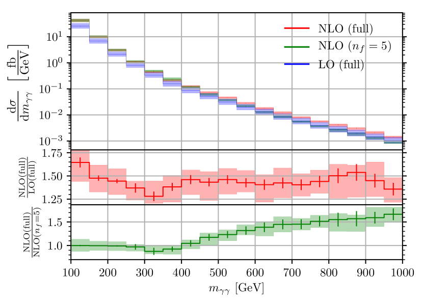
Figure 3: Diphoton invariant mass distribution (fixed order calculation), comparing the result with $n_{f}=5$ to the result including massive top quark loops. The lower panels show the ratios $\mathrm{NLO(full)}/\mathrm{LO(full)}$ and $\mathrm{NLO(full)}/\mathrm{NLO}(n_{f}=5)$. The shaded bands show the envelope of the 7-point scale variation as explained in the text. In the ratio plots, only the scale of the numerators is varied, while the scale of the denominators is fixed to $\mu_{R}=\mu_{F}=m_{\gamma\gamma}/2$. The bars indicate the uncertainty due to the numerical evaluation of the phase-space and loop integrals.

NRQCD amplitude

Numerical values for the coefficients ${\mathcal{A}}^{J}_{t,\{\lambda_{i}\}}$ at leading-order in $\alpha_{s}$ up to $J=4$ are given in Ref. Kawabata:2016aya . We have used them as a check of our numerical calculation of the Born amplitude.

We also evaluated the massive two-loop amplitude at $615$ phase space points with $m_{t}=173$ GeV in the ranges $0<\cos{}\left(\theta{}\right)<1$ and $0.001\leq{}\beta{}\leq{}0.2$, using the program pySecDec Borowka:2017idc ; Borowka:2018goh . The amplitude can numerically be fitted to a suitable ansatz in $\beta$ and $\cos\theta$. We have compared the coefficients of terms proportional to $\ln{(\beta)}$ to the known analytical results based on expanding equation (31) and find good agreement. Note that the coefficients of terms not proportional to $\ln{(\beta)}$ receive contributions from the unknown term $A^{(1)}(\theta)$ and can therefore not be checked this way.

4.2 Invariant mass distribution of the diphoton system

The distribution of the invariant mass of the photon pair is shown in Fig. 3 for invariant masses up to 1 TeV, where we show purely fixed order results at LO, at NLO with five massless flavours and at NLO including massive top quark loops. The ratio plots show the K-factor including the full quark loop content and the ratio between the full and the five-flavour NLO cross-section. We observe that the scale uncertainties are reduced at NLO, and that the top quark loops enhance the differential cross section for $m_{\gamma\gamma}$ values far beyond the top-quark pair-production threshold, asymptotically approaching the $n_{f}=6$ value Campbell:2016yrh .

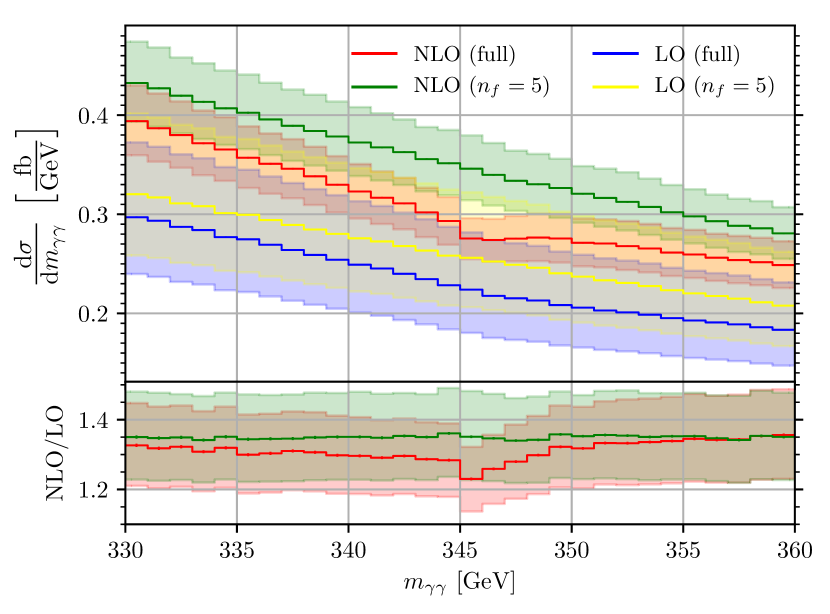
Figure 4: Zoom into the threshold region of the diphoton invariant mass distribution (fixed order calculation), showing the $n_{f}=5$ and full result separately. The shaded bands indicate the scale uncertainties, while the bars indicate uncertainties due to the numerical evaluation of the phase-space and loop integrals. The ratio plot in the lower panel shows the ratios $\mathrm{NLO(full)}/\mathrm{LO(full)}$ (red) and $\mathrm{NLO(}n_{f}=5\mathrm{)}/\mathrm{LO(}n_{f}=5\mathrm{)}$ (green), with the scale variation bands obtained by varying the scale in the numerators only.

In Fig. 4 we zoom into the threshold region, still showing fixed order results only. We can clearly see that after the top quark pair production threshold, the full result shows a dip and then changes slope, which is due to the fact that the two-loop amplitude contains the exchange of a Coulomb gluon (see top left diagram of Fig. 1), as explained in Section 3. In Ref. Kawabata:2016aya it was suggested that this characteristic “dip-bump structure” could be used for a determination of the top quark mass which is free from top quark reconstruction uncertainties, at least at the FCC where the statistical uncertainties for this process would be very small, and the systematic uncertainty due to the finite resolution of the photon energies and angles should be at least as good as at the LHC, where it is at the sub-percent level Aad:2014nim ; Khachatryan:2015iwa .

In Fig. 5 we show the $m_{\gamma\gamma}$-distribution in the threshold region which results from a combination of the fixed-order NLO (QCD) calculation with the resummation of Coulomb gluon exchanges as described in Section 3.2. The scale band in this figure are produced by varying only $\mu$, the scale associated to the renormalisation of the Green’s function. We observe that the dependence on the scale $\mu$ is considerably reduced at NLO compared to the leading-order matched cross-section. The scale band at NLO is comparable to the size of our numerical uncertainties. Further, our leading-order matched cross-section shows a milder dependence on $\mu$ than the one presented in Kawabata:2016aya . This is due to the inclusion of NLO-terms in the coefficient ${\mathcal{B}}_{t}(\beta)$, which have been omitted in Kawabata:2016aya .

We do not consider the effects from a colour-octet $t\bar{t}$ state because the corresponding Green’s function is monotonically increasing in the resonance region Kiyo:2008bv and therefore not expected to move the position of the dip significantly.

Now let us address the prospects to measure the top quark mass from the threshold behaviour of the $m_{\gamma\gamma}$ distribution. In Ref. Kawabata:2016aya it was argued that the characteristic dip-bump structure does not change its location in the $m_{\gamma\gamma}$ spectrum under scale variations, only the overall normalisation is changing. It was also anticipated that the inclusion of the fixed order two-loop amplitude would reduce this uncertainty. Indeed we find that the NLO corrections reduce the scale uncertainties due to 7-point $\mu_{R},\mu_{F}$-variations from about 20% at LO to just below the 10% level at NLO.

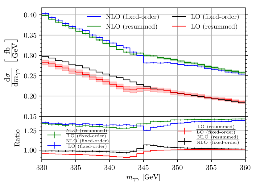
Figure 5: Zoom into the threshold region of the diphoton invariant mass distribution, comparing results with and without NRQCD. The shaded bands indicate the scale uncertainty by varying the scale $\mu$ by a factor of 2 around the central scale $\mu=80$ GeV. The renormalisation and the factorisation scales are set to $\mu_{R}=\mu_{F}=m_{\gamma\gamma}/2$ and not varied in this plot. The bars indicate uncertainties due to the numerical evaluation of the phase-space and loop integrals.

Figure 6: Effect of the top quark width on the dip-bump-structure at LO and NLO. The solid lines correspond to $\Gamma_{t}=1.367$ GeV, the dashed to $\Gamma_{t}=1.498$ GeV and the dotted to $\Gamma_{t}=0.5$ GeV. The corresponding scale bands are also shown in the upper plot.

The treatment of the top quark width included in the NRQCD calculation could be refined by including higher order corrections to the width. We have investigated how a change of the width affects the height and the location of the dip-bump-structure. We have performed the calculation with three different values for $\Gamma_{t}$: our default LO value of $\Gamma_{t}=1.498$ GeV, an NLO value of $\Gamma_{t}=1.367$ GeV, obtained using the expressions of Ref. Jezabek:1988iv , and an “extreme” value of $\Gamma_{t}=0.5$ GeV. The result is shown in Fig. 6. We observe that the amplitude of the dip-bump-structure is quite sensitive to the width, with small widths giving a larger dip-bump-amplitude. This feature might offer the possibility to constrain the top quark width based on a template fit to the $m_{\gamma\gamma}$ distribution, similar to what has been performed in Ref. ATLAS:2019onj for the $m_{lb}$ distribution. Furthermore, we found that at LO, the dip-bump-structure is less broad for smaller top quark widths, while with 1 GeV binnings this is not visible at NLO.

Our results show that the description of the region which is critical for the top quark mass measurement sensitively depends on the theoretical modelling. Therefore, without calculating even higher orders, it is diffcult to assess how large the uncertainties due to the theoretical description really are.

The experimental resolution at the LHC is estimated to be about $10\%/\sqrt{E_{\gamma}\,\rm{[GeV]}}$ Aad:2014nim ; Khachatryan:2015iwa . A resolution of the photon energy scale of about 0.5% or better leads to a systematic uncertainty on $m_{t}$ of about 1 GeV Kawabata:2016aya . Such an uncertainty is not competitive with current measurements from top quark pair production Castro:2019ttg . Therefore such a top quark mass determination has to wait for measurements at a future collider if at all feasible. In order to assess from the theory side whether the shape change present in our best theoretical prediction would be sufficient to measure the top quark mass, it would be useful to perform the current study for various top quark masses, which would enter an experimental template fit. However such an analysis is beyond the scope of this paper and we postpone it to future work.

5 Conclusions and Outlook

We have calculated the production of a photon pair in gluon fusion at order $\alpha_{s}^{3}$, including massive top quark loops. This calculation, which is NLO for the gluon initiated channel, is formally part of the N³LO corrections to the $pp\to\gamma\gamma$ process. However, the gluon channel is important at the LHC due to the large gluon luminosity. The top quark loops have a considerable impact on the diphoton invariant mass spectrum, at values of $m_{\gamma\gamma}$ larger than about 800 GeV they enhance the $m_{\gamma\gamma}$ differential cross section by more than 50%.

The region around the top quark pair production threshold in the diphoton invariant mass spectrum is particularly interesting. The fixed order amplitude has a divergence starting at two loops due to Coulomb gluon exchange. We have used NRQCD methods to resum the bound state effects in order to obtain a more reliable description of the threshold region. Matching the resummed calculation to our fixed order NLO calculation we observe a reduction of the renormalisation and factorisation scale uncertainties in the threshold region by more than a factor of two, and an even more drastic reduction of the scale uncertainty related to the renormalised NLO Green’s function.

These results are promising in view of the possibility of measuring the top quark mass from the characteristic behaviour of the diphoton invariant mass spectrum around the top quark pair production threshold. In Ref. Kawabata:2016aya , it was found that the LO resummed result shows a characteristic “dip-bump” structure and the conclusion was that this would allow a precise measurement of the top quark mass with the statistics and photon resolution projected for the FCC, once an NLO calculation is available such that the scale uncertainties are reduced. Now we indeed found that at NLO, the scale uncertainties are reduced. Furthermore, the characteristic “dip-bump” structure at NLO remains stable when switching from a LO value to an NLO value for the top quark width. A detailed assessment of whether this structure and the change in slope is pronounced enough for a top quark mass measurement once all channels contributing to this observable are included deserves further study. It also requires a detailed study of the prospective experimental uncertainties.

Furthermore, it would be interesting to investigate other top quark mass schemes, as well as the possibility to constrain the top quark width from this process. However this is beyond the scope of this paper and therefore we defer it to future work.

References

- (1) CMS collaboration, S. Chatrchyan et al., Measurement of differential cross sections for the production of a pair of isolated photons in pp collisions at , Eur. Phys. J. C74 (2014) 3129 [1405.7225].
- (2) ATLAS collaboration, M. Aaboud et al., Measurements of integrated and differential cross sections for isolated photon pair production in collisions at TeV with the ATLAS detector, Phys. Rev. D95 (2017) 112005 [1704.03839].
- (3) D. A. Dicus and S. S. D. Willenbrock, Photon Pair Production and the Intermediate Mass Higgs Boson, Phys. Rev. D37 (1988) 1801.
- (4) L. J. Dixon and M. S. Siu, Resonance continuum interference in the diphoton Higgs signal at the LHC, Phys. Rev. Lett. 90 (2003) 252001 [hep-ph/0302233].
- (5) S. P. Martin, Shift in the LHC Higgs diphoton mass peak from interference with background, Phys. Rev. D86 (2012) 073016 [1208.1533].
- (6) D. de Florian, N. Fidanza, R. J. Hernandez-Pinto, J. Mazzitelli, Y. Rotstein Habarnau and G. F. R. Sborlini, A complete calculation of the signal-background interference for the Higgs diphoton decay channel, Eur. Phys. J. C73 (2013) 2387 [1303.1397].
- (7) S. P. Martin, Interference of Higgs diphoton signal and background in production with a jet at the LHC, Phys. Rev. D88 (2013) 013004 [1303.3342].
- (8) L. J. Dixon and Y. Li, Bounding the Higgs Boson Width Through Interferometry, Phys. Rev. Lett. 111 (2013) 111802 [1305.3854].
- (9) J. Campbell, M. Carena, R. Harnik and Z. Liu, Interference in the On-Shell Rate and the Higgs Boson Total Width, Phys. Rev. Lett. 119 (2017) 181801 [1704.08259].
- (10) L. Cieri, F. Coradeschi, D. de Florian and N. Fidanza, Transverse-momentum resummation for the signal-background interference in the channel at the LHC, Phys. Rev. D96 (2017) 054003 [1706.07331].
- (11) ATLAS collaboration, M. Aaboud et al., Search for resonances in diphoton events at =13 TeV with the ATLAS detector, JHEP 09 (2016) 001 [1606.03833].
- (12) CMS collaboration, A. M. Sirunyan et al., Search for physics beyond the standard model in high-mass diphoton events from proton-proton collisions at 13 TeV, Phys. Rev. D98 (2018) 092001 [1809.00327].
- (13) S. R. Dugad, P. Jain, S. Mitra, P. Sanyal and R. K. Verma, The top threshold effect in the production at the LHC, Eur. Phys. J. C78 (2018) 715 [1605.07360].
- (14) S. Kawabata and H. Yokoya, Top-quark mass from the diphoton mass spectrum, Eur. Phys. J. C77 (2017) 323 [1607.00990].
- (15) T. Binoth, J. P. Guillet, E. Pilon and M. Werlen, A Full next-to-leading order study of direct photon pair production in hadronic collisions, Eur. Phys. J. C16 (2000) 311 [hep-ph/9911340].
- (16) C. Balazs, E. L. Berger, P. M. Nadolsky and C. P. Yuan, Calculation of prompt diphoton production cross-sections at Tevatron and LHC energies, Phys. Rev. D76 (2007) 013009 [0704.0001].
- (17) Z. Bern, A. De Freitas and L. J. Dixon, Two loop amplitudes for gluon fusion into two photons, JHEP 09 (2001) 037 [hep-ph/0109078].
- (18) Z. Bern, L. J. Dixon and C. Schmidt, Isolating a light Higgs boson from the diphoton background at the CERN LHC, Phys. Rev. D66 (2002) 074018 [hep-ph/0206194].
- (19) J. M. Campbell, R. K. Ellis and C. Williams, Vector boson pair production at the LHC, JHEP 07 (2011) 018 [1105.0020].
- (20) F. Maltoni, M. K. Mandal and X. Zhao, Top-quark effects in diphoton production through gluon fusion at NLO in QCD, 1812.08703.
- (21) M. Czakon, Tops from Light Quarks: Full Mass Dependence at Two-Loops in QCD, Phys. Lett. B664 (2008) 307 [0803.1400].
- (22) M. K. Mandal and X. Zhao, Evaluating multi-loop Feynman integrals numerically through differential equations, JHEP 03 (2019) 190 [1812.03060].
- (23) S. Caron-Huot and J. M. Henn, Iterative structure of finite loop integrals, JHEP 06 (2014) 114 [1404.2922].
- (24) M. Becchetti and R. Bonciani, Two-Loop Master Integrals for the Planar QCD Massive Corrections to Di-photon and Di-jet Hadro-production, JHEP 01 (2018) 048 [1712.02537].
- (25) A. von Manteuffel and L. Tancredi, A non-planar two-loop three-point function beyond multiple polylogarithms, JHEP 06 (2017) 127 [1701.05905].
- (26) J. Broedel, C. Duhr, F. Dulat, B. Penante and L. Tancredi, Elliptic polylogarithms and Feynman parameter integrals, JHEP 05 (2019) 120 [1902.09971].
- (27) U. Aglietti, R. Bonciani, G. Degrassi and A. Vicini, Analytic Results for Virtual QCD Corrections to Higgs Production and Decay, JHEP 01 (2007) 021 [hep-ph/0611266].
- (28) C. Anastasiou, S. Beerli, S. Bucherer, A. Daleo and Z. Kunszt, Two-loop amplitudes and master integrals for the production of a Higgs boson via a massive quark and a scalar-quark loop, JHEP 01 (2007) 082 [hep-ph/0611236].
- (29) S. Catani, L. Cieri, D. de Florian, G. Ferrera and M. Grazzini, Diphoton production at hadron colliders: a fully-differential QCD calculation at NNLO, Phys. Rev. Lett. 108 (2012) 072001 [1110.2375].
- (30) S. Catani, L. Cieri, D. de Florian, G. Ferrera and M. Grazzini, Diphoton production at the LHC: a QCD study up to NNLO, JHEP 04 (2018) 142 [1802.02095].
- (31) J. M. Campbell, R. K. Ellis, Y. Li and C. Williams, Predictions for diphoton production at the LHC through NNLO in QCD, JHEP 07 (2016) 148 [1603.02663].
- (32) M. Grazzini, S. Kallweit and M. Wiesemann, Fully differential NNLO computations with MATRIX, Eur. Phys. J. C78 (2018) 537 [1711.06631].
- (33) L. Chen, A prescription for projectors to compute helicity amplitudes in D dimensions, 1904.00705.
- (34) T. Ahmed, A. H. Ajjath, L. Chen, P. K. Dhani, P. Mukherjee and V. Ravindran, Polarised Amplitudes and Soft-Virtual Cross Sections for at NNLO in QCD, 1910.06347.
- (35) R. Karplus and M. Neuman, The scattering of light by light, Phys. Rev. 83 (1951) 776.
- (36) Z. Bern, A. De Freitas, L. J. Dixon, A. Ghinculov and H. L. Wong, QCD and QED corrections to light by light scattering, JHEP 11 (2001) 031 [hep-ph/0109079].
- (37) T. Binoth, E. W. N. Glover, P. Marquard and J. J. van der Bij, Two loop corrections to light by light scattering in supersymmetric QED, JHEP 05 (2002) 060 [hep-ph/0202266].
- (38) Z. Bern and A. G. Morgan, Massive loop amplitudes from unitarity, Nucl. Phys. B467 (1996) 479 [hep-ph/9511336].
- (39) C. Bernicot, Light-light amplitude from generalized unitarity in massive QED, 0804.0749.
- (40) S. Frixione, Z. Kunszt and A. Signer, Three jet cross-sections to next-to-leading order, Nucl. Phys. B467 (1996) 399 [hep-ph/9512328].
- (41) P. Nason, A New method for combining NLO QCD with shower Monte Carlo algorithms, JHEP 11 (2004) 040 [hep-ph/0409146].
- (42) S. Frixione, P. Nason and C. Oleari, Matching NLO QCD computations with Parton Shower simulations: the POWHEG method, JHEP 11 (2007) 070 [0709.2092].
- (43) S. Alioli, P. Nason, C. Oleari and E. Re, A general framework for implementing NLO calculations in shower Monte Carlo programs: the POWHEG BOX, JHEP 06 (2010) 043 [1002.2581].
- (44) S. P. Jones, Automation of 2-loop Amplitude Calculations, PoS LL2016 (2016) 069 [1608.03846].
- (45) A. von Manteuffel and C. Studerus, Reduze 2 - Distributed Feynman Integral Reduction, 1201.4330.
- (46) M. Argeri, S. Di Vita, P. Mastrolia, E. Mirabella, J. Schlenk, U. Schubert et al., Magnus and Dyson Series for Master Integrals, JHEP 03 (2014) 082 [1401.2979].
- (47) A. von Manteuffel, E. Panzer and R. M. Schabinger, A quasi-finite basis for multi-loop Feynman integrals, JHEP 02 (2015) 120 [1411.7392].
- (48) S. Borowka, G. Heinrich, S. Jahn, S. P. Jones, M. Kerner, J. Schlenk et al., pySecDec: a toolbox for the numerical evaluation of multi-scale integrals, Comput. Phys. Commun. 222 (2018) 313 [1703.09692].
- (49) S. Borowka, G. Heinrich, S. Jahn, S. P. Jones, M. Kerner and J. Schlenk, A GPU compatible quasi-Monte Carlo integrator interfaced to pySecDec, Comput. Phys. Commun. 240 (2019) 120 [1811.11720].
- (50) G. Luisoni, P. Nason, C. Oleari and F. Tramontano, /HZ + 0 and 1 jet at NLO with the POWHEG BOX interfaced to GoSam and their merging within MiNLO, JHEP 1310 (2013) 083 [1306.2542].
- (51) G. Cullen, N. Greiner, G. Heinrich, G. Luisoni, P. Mastrolia, G. Ossola et al., Automated One-Loop Calculations with GoSam, Eur. Phys. J. C72 (2012) 1889 [1111.2034].
- (52) G. Cullen et al., GS-2.0: a tool for automated one-loop calculations within the Standard Model and beyond, Eur. Phys. J. C74 (2014) 3001 [1404.7096].
- (53) W. E. Caswell and G. P. Lepage, Effective Lagrangians for Bound State Problems in QED, QCD, and Other Field Theories, Phys. Lett. 167B (1986) 437.
- (54) G. T. Bodwin, E. Braaten and G. P. Lepage, Rigorous QCD analysis of inclusive annihilation and production of heavy quarkonium, Phys. Rev. D51 (1995) 1125 [hep-ph/9407339].
- (55) A. Pineda and J. Soto, Effective field theory for ultrasoft momenta in NRQCD and NRQED, Nucl. Phys. Proc. Suppl. 64 (1998) 428 [hep-ph/9707481].
- (56) M. Beneke and V. A. Smirnov, Asymptotic expansion of Feynman integrals near threshold, Nucl. Phys. B522 (1998) 321 [hep-ph/9711391].
- (57) K. Melnikov, M. Spira and O. I. Yakovlev, Threshold effects in two photon decays of Higgs particles, Z. Phys. C64 (1994) 401 [hep-ph/9405301].
- (58) K. Melnikov and O. I. Yakovlev, Top near threshold: All alpha-S corrections are trivial, Phys. Lett. B324 (1994) 217 [hep-ph/9302311].
- (59) W. Fischler, Quark - anti-Quark Potential in QCD, Nucl. Phys. B129 (1977) 157.
- (60) A. Billoire, How Heavy Must Be Quarks in Order to Build Coulombic q anti-q Bound States, Phys. Lett. 92B (1980) 343.
- (61) M. Beneke, A Quark mass definition adequate for threshold problems, Phys. Lett. B434 (1998) 115 [hep-ph/9804241].
- (62) A. H. Hoang and T. Teubner, Top quark pair production at threshold: Complete next-to-next-to-leading order relativistic corrections, Phys. Rev. D58 (1998) 114023 [hep-ph/9801397].
- (63) M. Beneke, A. Signer and V. A. Smirnov, A Two loop application of the threshold expansion: The Bottom quark mass from b anti-b production, in Radiative corrections: Application of quantum field theory to phenomenology. Proceedings, 4th International Symposium, RADCOR’98, Barcelona, Spain, September 8-12, 1998, pp. 223–234, 1999, hep-ph/9906476.
- (64) A. H. Hoang, A. V. Manohar, I. W. Stewart and T. Teubner, The Threshold t anti-t cross-section at NNLL order, Phys. Rev. D65 (2002) 014014 [hep-ph/0107144].
- (65) A. Petrelli, M. Cacciari, M. Greco, F. Maltoni and M. L. Mangano, NLO production and decay of quarkonium, Nucl. Phys. B514 (1998) 245 [hep-ph/9707223].
- (66) K. Hagiwara, Y. Sumino and H. Yokoya, Bound-state Effects on Top Quark Production at Hadron Colliders, Phys. Lett. B666 (2008) 71 [0804.1014].
- (67) Kiyo, Y. and Kühn, Johann H. and Moch, S. and Steinhauser, M. and Uwer, P., Top-quark pair production near threshold at LHC, Eur. Phys. J. C60 (2009) 375 [0812.0919].
- (68) A. H. Hoang and C. J. Reisser, Electroweak absorptive parts in NRQCD matching conditions, Phys. Rev. D71 (2005) 074022 [hep-ph/0412258].
- (69) Y. Kiyo, A. Pineda and A. Signer, New determination of inclusive electromagnetic decay ratios of heavy quarkonium from QCD, Nucl. Phys. B841 (2010) 231 [1006.2685].
- (70) J. Butterworth et al., PDF4LHC recommendations for LHC Run II, 1510.03865.
- (71) S. Dulat, T.-J. Hou, J. Gao, M. Guzzi, J. Huston, P. Nadolsky et al., New parton distribution functions from a global analysis of quantum chromodynamics, Phys. Rev. D93 (2016) 033006 [1506.07443].
- (72) L. A. Harland-Lang, A. D. Martin, P. Motylinski and R. S. Thorne, Parton distributions in the LHC era: MMHT 2014 PDFs, Eur. Phys. J. C75 (2015) 204 [1412.3989].
- (73) NNPDF collaboration, R. D. Ball et al., Parton distributions for the LHC Run II, JHEP 04 (2015) 040 [1410.8849].
- (74) A. Buckley, J. Ferrando, S. Lloyd, K. Nordström, B. Page, M. Rüfenacht et al., LHAPDF6: parton density access in the LHC precision era, Eur. Phys. J. C75 (2015) 132 [1412.7420].
- (75) J. Campbell and T. Neumann, Precision Phenomenology with MCFM, 1909.09117.
- (76) G. ’t Hooft and M. J. G. Veltman, Regularization and Renormalization of Gauge Fields, Nucl. Phys. B44 (1972) 189.
- (77) ATLAS collaboration, G. Aad et al., Electron and photon energy calibration with the ATLAS detector using LHC Run 1 data, Eur. Phys. J. C74 (2014) 3071 [1407.5063].
- (78) CMS collaboration, V. Khachatryan et al., Performance of Photon Reconstruction and Identification with the CMS Detector in Proton-Proton Collisions at sqrt(s) = 8 TeV, JINST 10 (2015) P08010 [1502.02702].
- (79) M. Jezabek and J. H. Kuhn, QCD Corrections to Semileptonic Decays of Heavy Quarks, Nucl. Phys. B314 (1989) 1.
- (80) The ATLAS collaboration, Measurement of the top-quark decay width in top-quark pair events in the dilepton channel at TeV with the ATLAS detector, ATLAS-CONF-2019-038.
- (81) ATLAS, CMS collaboration, A. Castro, Top Quark Mass Measurements in ATLAS and CMS, in 12th International Workshop on Top Quark Physics (TOP2019) Beijing, China, September 22-27, 2019, 2019, 1911.09437.