Subfemtosecond glory hologrammetry for vectorial optical waveform reconstruction

Abstract

In this Letter, we propose a new method to characterize the temporal structure of arbitrary optical laser pulses with low pulse energies. This approach is based on strong field photoelectron holography with the glory rescattering effect as the underlying mechanism in the near-forward direction. Utilizing the subfemtosecond glory rescattering process as a fast temporal gate to sample the unknown light pulse, the time-dependent vectorial electric field can be retrieved from the streaking photoelectron momentum spectra. Our method avoids the challenging task of generation or manipulation of attosecond pulses and signifies important progress in arbitrary optical waveform characterization.

Probing or manipulation of ultrafast electron dynamics on a subfemtosecond($\leq 10^{-15}~{}s$) or attosecond($\sim 10^{-18}~{}s$) timescale necessitates ultrashort laser pulses lasting only a few or near-single optical cycles with controllable waveformsGoulielmakis et al. (2007); Kremer et al. (2009); Schiffrin et al. (2012); Ishii et al. (2014); Garg et al. (2016); Sommer et al. (2016); Rozen et al. (2019). Developments in frequency comb technology combined with pulse-shaping methods have allowed arbitrary electromagnetic waveforms to be synthesized at optical frequenciesDel’Haye et al. (2007); Jiang et al. (2007); Cundiff and Weiner (2010); Chan et al. (2011); Wirth et al. (2011); Schliesser et al. (2012). Knowledge of the temporal structure of these light pulses is a prerequisite for subsequent applications. Traditional characterization techniques, such as frequency-resolved optical gating(FROG), spectral phase interferometry for direct electric field reconstruction(SPIDER) or dispersion scan(d-scan), have been used to measure the spectral/temporal amplitude/phase or dispersion/chirp of short pulsesTrebino et al. (1997); Iaconis and Walmsley (1998); Miranda et al. (2012). However, the phase-matching problem of nonlinear crystals and the deficiency in determining the absolute phase(carrier-envelope phase, CEP) both limit their applicability. Instead, direct access to the time-domain electric field $\textbf{E}_{L}(t)$ requires a fast nonlinear response that is significantly shorter than an optical cycleWyatt et al. (2016); Park et al. (2018).

Advancements in strong field physics have provided such ultrashort temporal gates. One widely used technique is attosecond streak cameraSansone et al. (2006); Goulielmakis et al. (2004); Itatani et al. (2002); Boge et al. (2014): isolated attosecond extreme ultraviolet(XUV) pulses generated by higher-order harmonic generation(HHG) processes are used to ionize atomsLewenstein et al. (1994); Baltuska et al. (2003); Witting et al. (2012); Abel et al. (2009); Ferrari et al. (2010); Sola et al. (2006). The ejected photoelectrons are then streaked to different final energies by the test laser field whose waveform is to be measured. The temporal structure of both the test laser and the attosecond XUV pulse can be accurately reconstructed from the streaking photoelectron spectraMairesse and Quéré (2005); Lucchini et al. (2015). Two other all-optical characterization methods, petahertz optical oscilloscope and attosecond spatial interferometry, both utilize the subfemtosecond tunneling-recombination process during HHG generation as the temporal gate to sample the test optical laser fieldKim et al. (2013); Carpeggiani et al. (2017).

Although these recent characterization techniques yield good performance, their requirement of generation or manipulation of broadband isolated attosecond XUV pulses is still very challenging to meetWang et al. (2009); Krausz and Stockman (2014); Chini et al. (2014). In this Letter, we propose a new method to extract the waveforms of unknown laser pulses with commonly used strong near-infrared(NIR) table-top laser light as a pump field to irradiate the atoms. Our proposal utilizes facilities from the strong field ionization and strong field photoelectron holography(SFPH) fieldsHuismans et al. (2011), and information of the weak test laser pulses is imprinted in the holographic interference fringes of the final photoelectron momentum distribution(PMD).

A strong NIR laser is able to tunnel ionize atoms, and the liberated photoelectron may be driven back and elastically scatter off the parent ion at a later timeCorkum (1993). Concerning SFPH, strong field tunneling ionization plays the role of an atomic-level beamsplitter: after tunneling, part of the photoelectron wavepacket less impacted by the ionic Coulomb potential forms a reference wave. The other part, termed the signal wave, is steered around and scatters off the atomic core. The hologram stemming from interference of the reference and signal waves at the detector encodes spatiotemporal information about the interaction of the electron-ion system. Recently, the interpretation of SFPH has been improved by the discovery of the glory rescattering effect in strong field ionizationXia et al. (2018).

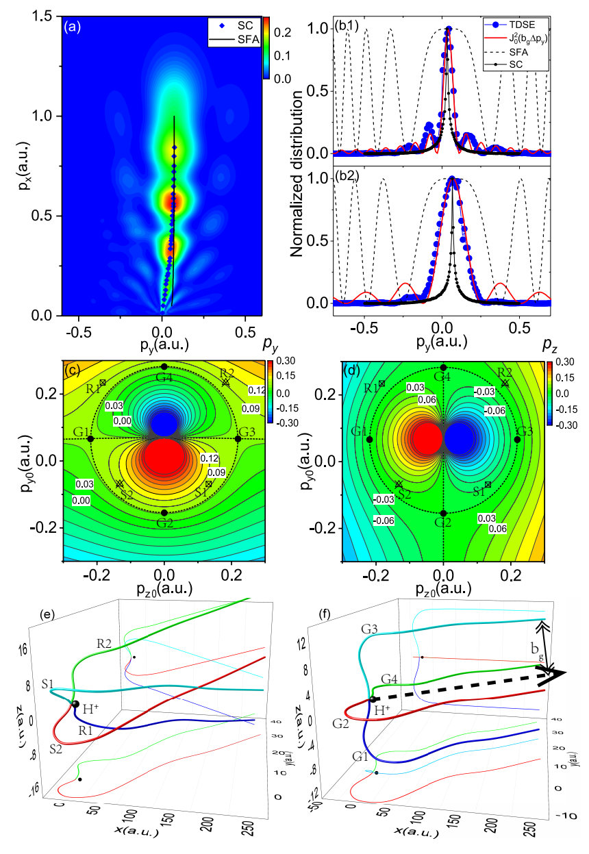
Figure 1: (a) PMD calculated using the TDSE in the polarization plane($p_{z}=0$), and ionization of H atoms by an OTC laser field. The glory interference maxima(GIM) estimated by the semiclassical method(SC, blue diamonds) and strong field approximation(SFA, black solid line) are also presented. (b1-b2) Normalized transverse momentum distribution with $p_{x}=$ 0.2(b1) and 0.6(b2). Note that the SFA curves have been shifted to match the peak positions calculated by the SC and TDSE. (c)(d) Contour plots of the deflection functions with $\eta_{0}=0.3$ and $p_{x}\approx 0.6$. The circle contour indicates the initial conditions of glory trajectories(GTs), while four typical GTs(G1, G2, G3 and G4) are shown in (f) with XY and XZ projections. (e)Two pairs of signal/reference trajectories with initial conditions from regions (S1, R1) and (S2, R2). See the text for more details.

For theoretical demonstration purposes, a fundamental pump laser field with a wavelength of $800nm$ and an intensity of $1.5\times 10^{14}W/cm^{2}$ is used to ionize hydrogen atoms: $\textbf{E}_{0}(t)=\epsilon_{0}\cos^{2}(\frac{\pi t}{T_{0}})\cos(\omega_{0}t)\mathbf{\hat{x}}$, where $T_{0}=3\times\frac{2\pi}{\omega_{0}}$, with the time duration only three optical cycles to eliminate multiple rescattering effects. Fig. 1(a) illustrates the PMD in the polarization plane simulated using the time-dependent Schrödinger equation(TDSE), with an orthogonally polarized two-color(OTC) laser field. The test laser pulse has a wavelength of $1600nm$, an intensity of $2.4\times 10^{11}W/cm^{2}$, and a time duration of four optical cycles: $\textbf{E}_{L}(t)=\epsilon_{L}\cos^{2}(\frac{\pi t}{T_{L}})\cos(\omega_{L}t)\mathbf{\hat{y}}$, with $T_{L}=4\times\frac{2\pi}{\omega_{L}}$. The spider-like interference fringes characteristic of SFPH are clearly visibleHuismans et al. (2011). Unless stated otherwise, atomic units will be used throughout.

Without considering the Coulomb potential, the phase difference responsible for the hologram between the signal and reference photoelectron waves can be derived using strong field approximation(SFA) or approximations from the path integral method as followsHuismans et al. (2011); Li et al. (2019); Brennecke and Lein (2019):

$$\delta\phi\approx\frac{1}{2}(\textbf{p}_{\perp}-\textbf{k}_{L})^{2}(t_{r}-t_{0}^{ref})$$ (1)

in which $\textbf{p}_{\perp}$ is the asymptotic photoelectron momentum perpendicular to the fundamental laser polarization. $t_{r}$ is the rescattering time, and $t_{0}^{ref}$ is the ionization time of the reference photoelectron wave. The intermediate canonical momentum between tunneling and rescattering is $\textbf{k}_{L}=-\frac{1}{t_{r}-t_{0}^{R}}\int^{t_{r}}_{t_{0}^{R}}\textbf{A}_{L}(t^{\prime})dt^{\prime}$ to ensure that the electron travels back to the ion, while $t_{0}^{R}$ is the ionization time of the rescattering wavepacket. Generally, for near-forward rescattering with a small transverse momentum $\textbf{p}_{\perp}$, the tunneling time for reference and rescattering(signal) quantum paths are approximately the same: $t_{0}^{ref}\approx t_{0}^{R}$. $\textbf{A}_{L}(t)=-\int^{t}\textbf{E}_{L}(t^{\prime})dt^{\prime}$ is the vector potential of the weak test laser field.

However, a $\cos(\mathcal{R}e(\delta\phi))$-like peak structure derived from Eqn. 1 for the transverse momentum distribution(black dashed lines in Fig. 1(b1)(b2) for different asymptotic longitudinal momenta $p_{x}=0.2,0.6$) fails to reproduce the TDSE results(blue dotted lines). This problem can be clarified from the semiclassical(SC) perspective of the Feynman path integral method, which dictates that the dominant contributions come from the regions around the classical trajectories. Fig. 1(c)(d) depict the contour plots of the deflection functions $\textbf{p}_{\perp}=\textbf{p}_{\perp}(\eta_{0},\textbf{p}_{\perp 0})$ obtained by solving Newton’s equation of motion after the electron emerges at $\eta_{0}=\omega_{0}t_{0}=\omega_{0}\mathcal{R}e(t_{0}^{ref})\approx 0.3$Liu (2014); Daněk et al. (2018). Due to Coulomb potential influence, the $p_{y0}\_p_{z0}$ plane can be divided into four signal/reference regional pairs: (S1, R1), (S2, R2), (S3, R3) and (S4, R4)(with the latter two not shown). For the final photoelectron momentum originating from inside these pairs, only two classical trajectories are found(Fig. 1(e)); however, infinite classical trajectories stemming from the circle contour dividing the signal and reference regions all contribute to the same asymptotic momentum(Fig. 1(f) depicts four such classical orbits).

This phenomenon is analogous to the (forward) glory effect in quantum scattering theoryFord and Wheeler (1959). The contributions of infinite so-called glory trajectories(GTs) to the final momentum distribution should be summed up. Referring to Eqn. 1, for simplicity, consider the case with only the NIR fundamental pulse; for a small deviation $\Delta p_{\perp}$ from the forward direction, we have $\Delta(\mathcal{R}e(\delta\phi))\sim\Delta p_{\perp}p_{\perp 0}(t_{r}-t_{0})\sim\Delta p_{\perp}b_{g}$, where $p_{\perp 0}\neq 0$ is the initial transverse momentum with the Coulomb potential involved. $b_{g}\sim p_{\perp 0}(t_{r}-t_{0})$ is interpreted as the asymptotic impact factor of GTs(Fig. 1(f))Xia et al. (2018). Then, the transverse momentum distribution in the near-forward direction is $f(p_{\perp})\propto|\frac{1}{2\pi}\int_{0}^{2\pi}e^{i\Delta p_{\perp}b_{g}\cos\theta}d\theta|^{2}=J_{0}^{2}(b_{g}\Delta p_{\perp})$. In an OTC field, this would result in $f(p_{\perp})\propto J_{0}^{2}(b_{g}|\textbf{p}_{\perp}-\textbf{p}_{L}|)$. $\textbf{p}_{L}$ is the transverse momenta corresponding to the primary glory interference maxima(GIM)(on the circle contour in Fig. 1(c)(d), $|\textbf{p}_{\perp}-\textbf{p}_{L}|\equiv 0$). This result has successfully interpreted the near-forward SFPH interference fringes in PMDXia et al. (2018); Brennecke and Lein (2019); López and Arbó (2019).

Using this SC photoelectron trajectory method, $b_{g}$ can be retrieved by back-propagation for each $p_{x}$Xia et al. (2018). The resulting squared-Bessel-like peak structure(red solid lines in Fig. 1(b1)(b2)) agrees very well with the TDSE simulation. A SC trajectory Monte Carlo simulation also reproduces the position of the GIM $\textbf{p}_{L}$(blue diamonds in Fig. 1(a), black dotted lines in Fig. 1(b1)(b2)). An approximation of this position can be found from Eqn. 1Tao et al. (2017): $\textbf{p}_{L}\approx\mathcal{R}e(\textbf{k}_{L})$. This result, shown in Fig. 1(a)(black solid line), describes the TDSE/SC simulations quite well, especially for larger longitudinal photoelectron momentum $p_{x}$. The deviation for smaller $p_{x}$ is due to the Coulomb effects.

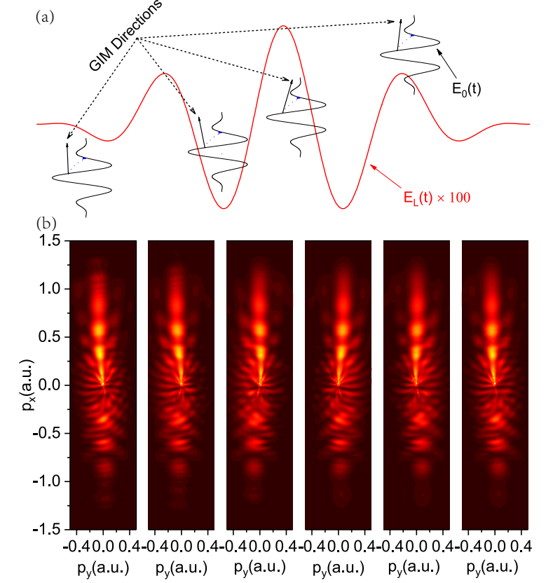
Figure 2: (a) Illustration of the sampling of a test laser field with the subfemtosecond glory rescattering process. Blue dashed arrows indicate the subcycle excursion of the tunneled electrons. (b) Integrated PMD simulated using the TDSE with time delay $\Delta\tau=\frac{n}{6}~{}o.c.$, where $n=-6,-4,-2,2,4,6$(left to right). $1~{}o.c.=\frac{2\pi}{\omega_{0}}$.

Therefore, adding a weak test laser $\textbf{E}_{L}$($\perp\textbf{E}_{0}$) introduces an extra factor into the phase difference between the reference and signal photoelectron waves(Eqn. 1) or, classically, slightly perturbs the whole bunch of glory rescattering trajectories(Fig. 1(f)). One of the consequences is a peak shift of the asymptotic transverse momentum distribution, the same as that in nondipole strong field ionization Tao et al. (2017); Ludwig et al. (2014); Wang et al. (2018); Daněk et al. (2018); He et al. (2017); Hartung et al. (2019). Therefore, we can utilize the subfemtosecond glory rescattering process as a fast temporal gate to sample a test laser pulse by varying the time delay between the fundamental and weak light pulses(Fig. 2(a)):

$$\textbf{p}_{L}(\Delta\tau)\approx\mathcal{R}e\{-\frac{1}{t_{r}-t_{0}^{R}}\int^{t_{r}+\Delta\tau}_{t_{0}^{R}+\Delta\tau}\textbf{A}_{L}(t)dt\}$$ (2)

Fig. 2(b) illustrates the TDSE simulation of PMDs with different time delays; the GIM oscillate with $\Delta\tau$. If the test light pulse does not contain frequency components that are larger than about $\omega_{0}$, we can derive the approximate waveform of the test light from the measured GIM as $\textbf{A}_{L}(t)\approx-\textbf{p}_{L}(t-t_{\alpha})+t^{2}_{\beta}\frac{d^{2}}{dt^{2}}\textbf{p}_{L}(t-t_{\alpha})$ for larger longitudinal momentum($p_{x}\sim(50\%-90\%)\times\frac{\epsilon_{0}}{\omega_{0}}$)Kübel et al. (2019), the second term on the right hand side is much smaller than the first in the present setup. $t_{\alpha,\beta}$ are small time parameters determined by the fundamental ionizing laser field(See the Supplementary for more details). Current experiments can measure the smallest transverse momentum amounting to that carried by a few photons, which is on the order of $\delta p_{c}\sim 10^{-3}~{}a.u.$Smeenk et al. (2011); Ludwig et al. (2014); Hartung et al. (2019). It is sufficient to resolve the peak positions in our scheme($\frac{\epsilon_{L}}{\omega_{L}}\gg\delta p_{c}$). In the following demonstrations we have also chosen the upper bound of the difference between two consecutively sampled peak shifts, estimated as $\delta p_{\perp}\sim\epsilon_{L}\frac{\sinh\omega_{L}t_{i}}{\omega_{L}t_{i}}\delta t$, to be slightly larger: $\delta p_{\perp}\gtrsim\delta p_{c}$, where $t_{i}=\mathcal{I}m(t_{0}^{R})$ and $\delta t$ is the time-step associated with changing the time delay between the fundamental and test laser fields.

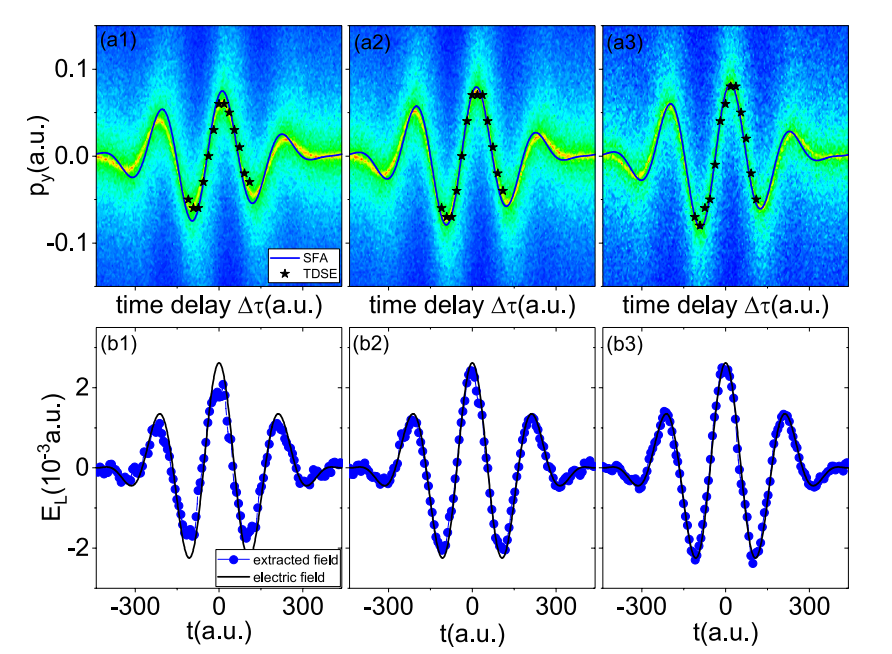
Figure 3: (a1-a3) Streaking spectra of the photoelectron momentum along the test laser polarization direction versus time delay for $p_{x}=$ 0.4(a1), 0.6(a2) and 0.8(a3). The TDSE results(black stars) well fit the SC trajectory Monte Carlo simulation results. Blue solid lines are estimated using Eqn. 2. (b1-b3) Corresponding electric fields(blue dotted lines) extracted from the GIM compared with the actual field(black solid lines).

The streaking photoelectron spectra of the transverse momentum distribution versus time delay are presented in Fig. 3(a1)(a2)(a3) for different final longitudinal momenta $p_{x}=0.4,0.6,0.8$. The same test laser light is used as in Fig. 1. TDSE results(black stars) agree very well with the SC simulation results. The SFA calculation yields a good approximation(blue solid lines in Fig. 3(a1)(a2)(a3)). More precisely, the electric field of the test laser pulse can be directly solved from Eqn. 2:

$$\textbf{E}_{L}(t)=\frac{1}{i\pi}\int_{-\infty}^{\infty}\frac{\omega\tilde{\textbf{p}}_{L}(\omega)}{a(\omega)+a^{\ast}(-\omega)}e^{i\omega t}d\omega$$ (3)

$\tilde{\textbf{p}}_{L}(\omega)=\int_{-\infty}^{\infty}\textbf{p}_{L}(\Delta\tau)e^{-i\omega\Delta\tau}d\Delta\tau$ is the corresponding Fourier transform, and $a(\omega)=-\int_{t_{0}^{R}}^{t_{r}}e^{i\omega t^{\prime}}dt^{\prime}/(t_{r}-t_{0}^{R})$. The extracted electric field is depicted as blue dotted lines in Fig. 3(b1)(b2)(b3). It reproduces the original test laser electric field(black solid lines).

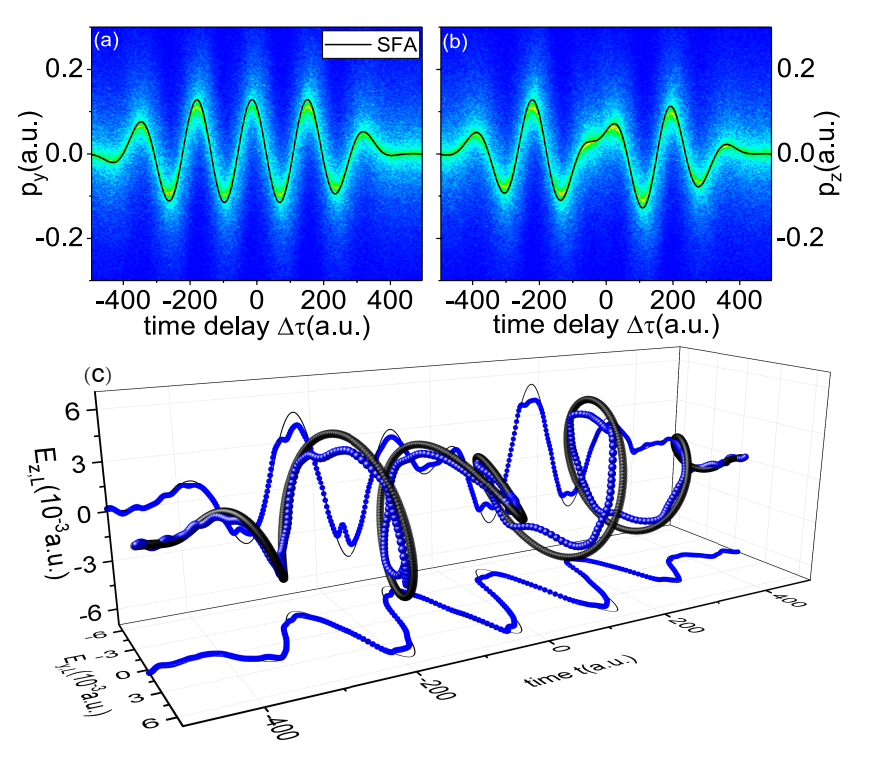
Figure 4: (a-b) Streaking photoelectron momentum spectra for two independent polarization directions of the synthesized test laser light with time-varying ellipticity($p_{x}=0.8$). (c) 3D representation of the extracted electric field(blue spheres). The result is compared to the synthesized waveform(black spheres); the reconstructed electric fields in the $\mathbf{\hat{y}}$ and $\mathbf{\hat{z}}$ directions(blue dotted lines) are also shown in the projections, alongside the respective actual fields(black solid lines).

The test optical laser is superposed on the fundamental pump pulse with perpendicular polarization, and in principle, the waveform of a test laser pulse with complex polarization states can be measured and reconstructedCarpeggiani et al. (2017). As an example, the streaking photoelectron spectra in two independent polarization directions are shown in Fig. 4(a)(b) for a light pulse with time-varying ellipticity synthesized by two counter-propagating circularly polarized laser beams: $\textbf{E}_{l}=\epsilon_{L}f_{L}(t-t_{d}/2)(\cos(\omega_{L}t+\frac{\pi}{4})\mathbf{\hat{y}}+\sin(\omega_{L}t+\frac{\pi}{4})\mathbf{\hat{z}})$ and $\textbf{E}_{r}=\epsilon_{L}f_{L}(t+t_{d}/2)(\cos(\omega_{L}t+\frac{\pi}{4})\mathbf{\hat{y}}-\sin(\omega_{L}t+\frac{\pi}{4})\mathbf{\hat{z}})$. The same retrieval algorithm is used to simultaneously extract the two electric fields(Fig. 4(c)). For all of these complex test light conditions, our method yields good results. In the frequency domain, we have the relationship $\tilde{\textbf{p}}_{L}(\omega)=r(\omega)\tilde{\textbf{A}}_{L}(\omega)$, the amplitude of the frequency response function $r(\omega)$ is approximately unity until up to about $\omega_{0}$, so although for demonstration purposes we have mostly used near-monochromatic pulses, this approach is also suitable for retrieval of optical waveforms with broad spectral bandwidths. By decreasing the wavelength of the fundamental ionizing laser field to, e.g. $400nm$, this method can be used to measure the electromagnetic waveforms in the visible, infrared and even terahertz regimes. Moreover, even though the proposed procedure requires that the time delay $\Delta\tau$ be continuously varied, single-shot measurement may be achieved by distributing the atoms spatially and using the spatial dependence of the propagating electromagnetic wave $A(\omega t-\textbf{k}\cdot\textbf{r})$ to provide the time delay, where $k=\omega/c$ is the wave vector.

In conclusion, by leveraging the subfemtosecond Coulomb glory rescattering effect as a fast temporal gate, we can sample arbitrary optical waveforms directly in the time domain with electron spectroscopy and reconstruct the temporal structure of the vectorial optical laser pulses. Our method completely avoids the use of attosecond XUV optics, and a conventional experimental setup related to strong field ionization research is sufficient to provide the required data. Our results will facilitate the study of ultrafast electron dynamics in attosecond physics.