High-Temperature Superconductivity in the Ti–H System at High Pressures

Abstract

Search for stable high-pressure compounds in the Ti–H system reveals the existence of titanium hydrides with new stoichiometries, including Ibam-Ti₂H₅, I4/m-Ti₅H₁₃, I$\bar{4}$-Ti₅H₁₄, Fddd-TiH₄, Immm-Ti₂H₁₃, P$\bar{1}$-TiH₁₂, and C2/m-TiH₂₂. Our calculations predict I4/mmm $\rightarrow$ R$\bar{3}$m and I4/mmm $\rightarrow$ Cmma transitions in TiH and TiH₂, respectively. Phonons and the electron–phonon coupling of all searched titanium hydrides are analyzed at high pressure. It is found that Immm-Ti₂H₁₃ rather than the highest hydrogen content C2/m-TiH₂₂, exhibits the highest superconducting critical temperature T_c. The estimated T_c of Immm-Ti₂H₁₃ and C2/m-TiH₂₂ are respectively 127.4–149.4 K ($\mu^{*}$=0.1-0.15) at 350 GPa and 91.3–110.2 K at 250 GPa by numerically solving the Eliashberg equations. One of the effects of pressure on T_c can be attributed to the softening and hardening of phonons with increasing pressure.

I Introduction

Enthusiasm for discovering high-temperature superconductors never cease Ginzburg (1999), since solid mercury was discovered to have zero electrical resistance below 4.2 K in 1911Van Delft and Kes (2010). In recent years, especially at high pressure, the record of the critical temperature (T_c) of superconductivity has been quickly and repeated to be broken in both experimental and theoretical studies, rendering the ultimate goal for synthesizing a room-temperature superconductor (T_c at around 298 K) appears to be within reach. In 2014, first-principles calculationDuan et al. (2014) based on density functional theory (DFT) predicted the T_c of Im$\bar{3}$m-H₃S to be around 191 K–204 K at 200 GPa. Subsequently, diamond anvil cell (DAC) experiment in 2015Drozdov et al. (2015) verified this prediction and reported the T_c of sulfur hydride of 203 K by compressing hydrogen sulfide to 150 GPa. In 2017, DFT calculationLiu et al. (2017) estimated T_c of Fm$\bar{3}$m-LaH₁₀ to be 274–286 K at 210 GPa and of Fm$\bar{3}$m-YH₁₀ to be 305–326 K (the highest theoretically-calculated T_c for simple binary systems so farBi et al. (2019)) at 250 GPa. Soon afterwards, the teams of HemleySomayazulu et al. (2019) and EremetsDrozdov et al. (2019) observed lanthanum hydride (Fm$\bar{3}$m-LaH₁₀) superconducting under the pressure (170-200 GPa) at around 250–260 K, which is the highest T_c that has been experimentally confirmed. Although the effect of pressure on superconductivity is not fully understoodLorenz and Chu (2005); Gao et al. (1994), these new record high-T_c superconductors are conventional, phonon-mediated ones. Based on Bardeen–Cooper–Schrieffer (BCS) or Migdal–Eliashberg theories, the pressure affects the T_c by making impact on the electronic and phonon parameters, e.g. electronic density of states at the Fermi level, average phonon frequency, and electron-phonon coupling (EPC) constant.

Motivation for investigating superconductivity of hydrides under pressure originally came from both the possibility that metallic hydrogen under high pressure could be a high-temperature superconductorAshcroft (1968) and from the viewpoint that the pressure of metallization of hydrogen-rich solids can be considerably lower than that of pure hydrogenAshcroft (2004a, b). Since carrying out the high-pressure experiments is expensive and technically challenging, many of the investigations on these superconductors are performed using calculations and crystal structure prediction techniques. Besides Im$\bar{3}$m-H₃S, Fm$\bar{3}$m-LaH₁₀ and Fm$\bar{3}$m-YH₁₀ (mentioned above), the calculated T_c of some predicted structures are as follows: R$\bar{3}$m-LiH₆ is 82 K at 300 GPaXie et al. (2014), Im$\bar{3}$m-MgH₆ is 271 K at 400 GPaFeng et al. (2015), Im$\bar{3}$m-CaH₆ is 220–235 K at 150 GPaWang et al. (2012), I4₁md-ScH₉ is 233 K at 300 GPaAbe (2017), Cmcm-ZrH is 11 K at 120 GPaLi et al. (2017), P2₁/m-HfH₂ is 11–13 K at 260 GPaLiu et al. (2015), Fdd2-TaH₆ is 124–136 K at 300 GPaZhuang et al. (2017), Pm$\bar{3}$m-GeH₃ is 140 K at 180 GPaGao et al. (2010), P6/mmm-LaH₁₆ is 156 K at 200 GPaKruglov et al. (2018), C2/m-SnH₁₄ is 86–97 K at 300 GPaEsfahani et al. (2016), Im$\bar{3}$m-H₃Se is 131 at 200 GPaFlores-Livas et al. (2016), P6/mmm-H₄Te is 95–104 at 170 GPaZhong et al. (2016). Almost all binary hydrides systems have been computationally studied by now, at least crudely, see an overview in Ref. Semenok et al., 2018.

Transition metal hydrides can form a variety of stable stoichiometries and have lower metallization pressure compared with other hydrides. Especially, those with high hydrogen content often contain unexpected hydrogen groups and exhibit intriguing properties. Titanium is such transition metal that inspires us to study the titanium hydrides under high pressure. At ambient conditions, TiH₂ crystallizes in a tetragonal structure (I4/mmm), which transforms into a cubic phase (Fm$\bar{3}$m) at temperature increasing to 310 KYakel (1958); San-Martin and Manchester (1987). DAC experimentsVennila et al. (2008); Kalita et al. (2010); Endo et al. (2013) indicated that I4/mmm-TiH₂ remains stable at the pressure up to 90 GPa at ambient temperature. The theoretically estimated T_c is 6.7 K ($\lambda$=0.84, $\mu^{*}$=0.1) for Fm$\bar{3}$m-TiH₂ and 2 mK ($\lambda$=0.22, $\mu^{*}$=0.1) for I4/mmm-TiH₂Shanavas et al. (2016) at ambient pressure.

In this paper, the crystal structures and superconductivity of titanium hydrides at pressures up to 350 GPa are systematically studied. In addition to I4/mmm-TiH₂, several new stoichiometries and phases are found at high pressure by a first-principles evolutionary algorithm. The predicted TiH₂₂ becomes thermodynamically stable at pressure above 235 GPa and contains H₂₀ units in its crystal structure. The dynamical stability of all high-pressure phases was verified by calculations of phonons throughout the Brillouin zone. Three different approaches are utilized to determine the superconducting T_c. The predicted T_c (numerical solution from the Eliashberg equations) for C2/m-TiH₂₂ and Immm-Ti₂H₁₃ are 91.3–110.2 K (at 250 GPa) and 127.4–149.4 K (at 350 GPa), respectively. Our work provides clear guidance for future experimental investigation of potential high-temperature superconductivity in titanium hydrides under pressure.

II Computational methodology

Variable-compositional prediction of stable compounds in the Ti–H system was performed at 0, 50, 100, 150, 200, 250, 300, and 350 GPa through first-principles evolutionary algorithm (EA), as implemented in the USPEX codeOganov and Glass (2006); Oganov et al. (2011); Lyakhov et al. (2013). Structure relaxations were based on DFT within the Perdew–Burke–Ernzerhof (PBE) generalized gradient approximation (GGA) exchange–correlation functionalPerdew et al. (1996), as implemented in the VASP packageKresse and Furthmüller (1996). The initial generation consisting of 120 structures was created using random symmetric generator. Structures in the following generations were created from the previous generation using heredity (40%), lattice mutation (20%), random symmetric generator (20%) and transmutation (20%) operators. The electron–ion interaction was described by projector-augmented wave (PAW) potentialsBlöchl (1994); Kresse and Joubert (1999), with 3p⁶4s²3d⁴ and 1s² shells treated as valence for Ti and H, respectively. Structures predicted to be stable or low-enthalpy metastable were then carefully reoptimized to construct convex hull and phase diagram at each pressure. Brillouin zone (BZ) was sampled using $\Gamma$-centered uniform k-meshes (2$\pi\times 0.05$ Å^-1) and the kinetic energy cutoff for the plane-wave basis set was 600 eV.

Phonon calculations were carried out using the finite-displacement method as implemented in the Phonopy Togo et al. (2008) codes, using VASP to calculate the force constants matrix, as well as density functional perturbation theory (DFPT)Baroni et al. (2001) in the Quantum ESPRESSO (QE) packageGiannozzi et al. (2009, 2017). Results of these two methods were in perfect agreement. The EPC coefficients were calculated using DFPT in QE, the norm-conserving pseudopotentials (tested by comparing the phonon spectra with the results calculated from Phonopy codes) and the PBE functional were used. Convergence tests show that 120 Ry is a suitable cutoff energy for the plane wave basis set in the QE calculation. A 4$\times$4$\times$4 q-mesh was used in the phonon and electron–phonon calculations.

T_c is estimated using three approaches: by numerically solving Eliashberg equations, and solving approximate Allen–Dynes formula, and the (latter-)modified McMillan formula. Starting from BCS theory, several first-principles Green’s function methods had been proposed to calculate the superconducting properties. Migdal–Eliashberg formalism is one of these, and can accurately describe conventional superconductorsGrimaldi et al. (1999). Within the Migdal approximationMigdal (1958), the adiabatic ratio $\lambda$$\omega$_D/$\epsilon$_F ($\simeq$$\sqrt{m^{*}/M}$) is small, since the vertex correction O($\sqrt{m^{*}/M}$) can compare to the bare vertex and then be neglected. In the adiabatic ratio, m^∗ is the electron effective mass, M is the ion mass, $\omega$_D is Debye frequency and $\epsilon$_F is Fermi energy. Then, T_c can be calculated by solving two nonlinear Eliashberg equations (or isotropic gap equations) for the Matsubara gap (or superconducting order parameter) $\Delta$_n$\equiv$$\Delta$(i$\omega$_i) and electron mass renormalization function (or wavefunction renormalization factor) Z_n$\equiv$Z(i$\omega$_i) along the imaginary frequency axis (i=$\sqrt{-1}$),

$${\textstyle\Delta_{n}Z_{n}=\frac{\pi}{\beta}\sum_{m=-M}^{M}\frac{\lambda(\omega_{n}-\omega_{m})-\mu^{*}\theta(\omega_{c}-|\omega_{m}|))}{\sqrt{\omega_{m}^{2}+\Delta_{m}^{2}}}\Delta_{m}}$$ (1)

and

$${\textstyle Z_{n}=1+\frac{\pi}{\beta\omega_{n}}\sum_{m=-M}^{M}\frac{\lambda(\omega_{n}-\omega_{m})}{\sqrt{\omega_{m}^{2}+\Delta_{m}^{2}}}\omega_{m}},$$ (2)

where $\beta$=1/k_BT, k_B is the Boltzmann constant, $\mu^{*}$ denotes the Coulomb pseudopotential, $\theta$ is the Heaviside function, $\omega_{c}$ is the phonon cut off frequency: $\omega_{c}$=3$\omega_{\textit{max}}$, $\omega_{max}$ is the maximum phonon frequency, $\omega_{n}$=($\pi/\beta$)(2n-1) is the nth fermion Matsubara frequency with n=0,$\pm$1,$\pm$2,…, the pairing kernel for electron–phonon interaction possesses the form $\lambda(\omega_{n}-\omega_{m})=2\int_{0}^{\omega_{\textit{max}}}\frac{\alpha^{2}F(\omega)\omega}{\omega^{2}+(\omega_{n}-\omega_{m})^{2}}d\omega$ and $\alpha^{2}F(\omega)$ represents the Eliashberg spectral function. A derivation of isotropic Eliashberg gap equations was given in detail by Allen and MitrovićAllen and Mitrović (1983). The important feature of the gap equations is that all the involved quantities only depend on the normal state, and then can be calculated first principles. At each temperature T, the coupled equations need to be solved iteratively until self-consistency. T_c is defined as the temperature at which the Matsubara gap $\Delta$_n becomes zero. The Eliashberg equations have been solved numerically for 2201 Matsubara frequencies (M=1100), in this paper. A detailed discussion of this numerical method was presented in Refs. Szczesniak, 2006; Szcze et al., 2012.

In addition to the above numerical method, T_c can also be obtained by other two analytical formulas. The first one was introduced by Allen and Dynes and the second one was initially proposed by McMillan and later modified by them. The former formula is given as:

$${\textstyle T_{c}=f_{1}f_{2}\frac{\omega_{\textit{log}}}{1.20}\textit{exp}\left(-\frac{1.04(1+\lambda))}{\lambda-\mu^{*}(1+0.62\lambda)}\right)},$$ (3)

where the logarithmic average frequency is defined as $\omega_{\textit{log}}=\textit{exp}\left(\frac{2}{\lambda}\int_{0}^{\omega_{\textit{max}}}d\omega\frac{\alpha^{2}F(\omega)}{\omega}\textit{ln}(\omega)\right)$, the isotropic EPC constant, which is a dimensionless measure of the average strength of the EPC, can be defined as: $\lambda=2\int_{0}^{\omega_{\textit{max}}}d\omega\frac{\alpha^{2}F(\omega)}{\omega}$, and f₁ and f₂ are strong coupling correction and shape correction, respectively. These two factors are

$${\textstyle f_{1}=\left\{1+\left[\frac{\lambda}{2.46(1+3.8\mu^{*}))}\right]^{\frac{3}{2}}\right\}^{\frac{1}{3}}}$$ (4)

and

$${\textstyle f_{2}=1+\frac{\left(\frac{\bar{\omega}_{2}}{\omega_{\textit{log}}}-1\right)\lambda^{2}}{\lambda^{2}+3.312(1+6.3\mu^{*})^{2}\left(\frac{\bar{\omega}_{2}}{\omega_{\textit{log}}}\right)^{2}}},$$ (5)

here, $\bar{\omega}_{2}$ is defines as: $\bar{\omega}_{2}=\left(\frac{2}{\lambda}\int_{0}^{\omega_{\textit{max}}}d\omega\alpha^{2}F(\omega)\omega\right)^{\frac{1}{2}}$. Generally, when $\lambda$ is small, the correction factors f₁ and f₂ are negligible. Therefore, requiring f₁f₂ to be 1 gives the Allen–Dynes modified McMillan equation (only changing a prefactor from $\frac{\Theta_{D}}{1.45}$ in McMillan equation to $\frac{\omega_{\textit{log}}}{1.2}$),

$${\textstyle T_{c}=\frac{\omega_{\textit{log}}}{1.20}\textit{exp}\left(-\frac{1.04(1+\lambda))}{\lambda-\mu^{*}(1+0.62\lambda)}\right)}.$$ (6)

Regardless of which of the above three methods is used to calculate T_c, two main input quantities are needed. One is the Coulomb pseudopotential $\mu^{*}$, which models the depairing interaction between the electrons. However, $\mu^{*}$ is hard to calculate from first principles. Herein, we used standard values $\mu^{*}$=0.1 and 0.15. Another one is the Eliashberg spectral function $\alpha^{2}F(\omega)$, which models the coupling of phonons to electrons on the Fermi surface. $\alpha^{2}F(\omega)$ can be calculated asChan et al. (2012)

$${\textstyle\alpha^{2}F(\omega)=\frac{1}{2\pi N(\epsilon_{F})}\sum_{\mathbf{q}\nu}\delta(\omega-\omega_{\mathbf{q}\nu})\frac{\gamma_{\mathbf{q}\nu}}{\omega_{\mathbf{q}\nu}}},$$ (7)

where N($\epsilon_{F}$) is the density of states at the Fermi level per unit cell per spin, $\mathbf{q}$ is the wavevector, $\omega_{\mathbf{q}}$ is the $\mathbf{q}$-point weight, $\omega_{\mathbf{q}\nu}$ is the screened phonon frequency, and $\gamma_{\mathbf{q}\nu}$ is the phonon linewidth, which is determined exclusively by the electron–phonon matrix elements $g_{mn}^{\nu}(\mathbf{k},\mathbf{q})$ with states on the Fermi surface, is given as:

$$\begin{split}\text{$\gamma_{\mathbf{q}\nu}$}=&\text{$\pi\omega_{\mathbf{q}\nu}\sum_{mn}\sum_{\mathbf{k}}\omega_{\mathbf{k}}\left|g_{mn}^{\nu}(\mathbf{k},\mathbf{q})\right|^{2}\delta(\epsilon_{m,\mathbf{k}+\mathbf{q}}-\epsilon_{F})$}\\ &\text{$\times\delta(\epsilon_{n,\mathbf{k}}-\epsilon_{F})$},\end{split}$$ (8)

where $\omega_{\mathbf{k}}$ is the $\mathbf{k}$-point weight normalized to 2 in order to account for the spin degeneracy in spin-unpolarized calculations. $g_{mn}^{\nu}(\mathbf{k},\mathbf{q})$ is described as:

$${\textstyle g_{mn}^{\nu}(\mathbf{k},\mathbf{q})=\left(\frac{\hbar}{2M\omega_{\mathbf{q}\nu}}\right)^{1/2}\left\langle m,\mathbf{k}+\mathbf{q}|\delta_{\mathbf{q}\nu}V_{SCF}|n,\mathbf{k}\right\rangle},$$ (9)

here, $|n,k\rangle$ is the bare electronic Bloch state, M is the ionic mass, and $\delta_{\mathbf{q}\nu}V_{SCF}$ is the derivative of the self-consistent potential with respect to the collective ionic displacement corresponding to the phonon wavevector $\mathbf{q}$ and mode $\nu$. In this work, $g_{mn}^{\nu}(\mathbf{k},\mathbf{q})$ is calculated within the harmonic approximation, using QE package.

III Results and discussions

Figure 1: (Color online) Convex-hull diagrams for the Ti–H system at (a) 0, (b) 50, (c) 100, (d) 150, (e) 200, (f) 250, (g) 300, and (h) 350 GPa. The blue dashed convex hull at 0 GPa shows the experimental resultChase (1998). Black lines with solid squares and red lines with open squares, respectively, represent the calculated results with and without including ZPE. The structures indicted in grey are those that lose stability after considering ZPE.

Thermodynamic convex hulls for the Ti–H system at several pressures are shown in Fig.1. In our structure searching, experimentally reported I4/mmm-TiH₂ is found to be the only stable phase at zero pressure. Lattice parameters were optimized to be a=3.208 Å and c=4.203 Å at 0 GPa, which is in good accordance with the experimental data (a=3.163 Å and c=4.391 Å)Vennila et al. (2008). The calculated Gibbs free energy of formation of I4/mmm-TiH₂ is -0.3123 eV/atom at zero pressure and 298 K [red convex hull in Fig. 1(a)], which is in good agreement with the experimental value of -0.363 eV/atom Chase (1998) [blue dashed convex hull in Fig. 1(a)]. Besides I4/mmm-TiH and Fm$\bar{3}$m-TiH₃, which were already predicted by ZhuangZhuang et al. (2018) under high pressure, several other phases and stoichiometries, including R$\bar{3}$m-TiH, Cmma-TiH₂, Ibam-Ti₂H₅, I4/m-Ti₅H₁₃, I$\bar{4}$-Ti₅H₁₄, Fddd-TiH₄, Immm-Ti₂H₁₃, P$\bar{1}$-TiH₁₂, C2/m-TiH₁₄ and C2/m-TiH₂₂, are predicated at pressures up to 350 GPa. No subhydrides (Ti_xH_y, $x>y$) show up in the Ti–H system at any pressure. The enthalpies of formation with and without including zero-point energy (ZPE) are depicted by red lines with open squares and black lines with solid squares in Fig.1(b)–(h), respectively. Taking ZPE into account did not significantly change the basic shape of convex hulls, but did introduce some changes of the data at pressures above 250 GPa: considering ZPE made I$\bar{4}$-Ti₅H₁₄ and P$\bar{1}$-TiH₁₂ metastable [indicated in grey in Fig. 1(f)–(h)] instead of stable structures above 250 GPa.

Figure 2: (Color online) Pressure–composition phase diagram of the Ti–H system at pressure up to 350 GPa.

The pressure–composition phase diagram of Ti–H system is depicted in Fig. 2. Based on our calculations, the phase transition sequence of Ti under high pressure is $\emph{P}6/\emph{mmm}(\omega)\xrightarrow{104\ \text{GPa}}\emph{Cmcm}(\gamma)\xrightarrow{109\ \text{GPa}}\emph{Cmcm}(\delta)\xrightarrow{127\ \text{GPa}}\mathit{Im}\bar{3}\mathit{m}(\beta)$. Although both $\gamma$-Ti and $\delta$-Ti have the same space group and contain 4 titanium atoms in their unit cell, the structure of $\gamma$-Ti is a distortion of $\omega$-Ti (hcp), while $\delta$-Ti, which is a body-centered one, is more similar to $\beta$-Ti (bcc). Under high pressure, P6₃/m-H transforms into C2/c-H at 110 GPa and further into Cmca-H at 280 GPa. The crystal structures of these high-pressure structures are shown in Fig. 3, and their structural parameters are listed in the Table S1 in Supplemental Material.

For TiH, it should be noted that the enthalpy of P4₂/mmc-TiH is lower than that of I4/mmm-TiH between 0-8 GPa [see also Fig. 4] which is consistent with the aforementioned calculationZhuang et al. (2018). However, P4₂/mmc-TiH is not thermodynamically stable from 0 to 8 GPa. With pressure increasing to 18 GPa, TiH (I4/mmm) begins to become stable and transforms into R$\bar{3}$m-TiH at 230 GPa. In addition, the calculations reveal a tetragonal (I4/mmm) to orthorhombic (Cmma) phase transition in TiH₂ at 78 GPa. The high-pressure Cmma-TiH₂ persists up to 298 GPa, above which TiH₂ is unstable. Note that enthalpy difference of Cmma-TiH₂ and P4/nmm-TiH₂ is very small, due to the similarity of these two structures.

Figure 3: (Color online) Crystal structures of titanium hydrides. Large spheres represent titanium atoms and small ones represent hydrogen atoms.

Figure 4: (Color online) Enthalpy as a function of pressure (without ZPE) for phases of (a) TiH, referenced to the I4/mmm-TiH phase, and (b) TiH₂, referenced to the I4/mmm-TiH₂ one.

The structure of Fm$\bar{3}$m-TiH₃ has an fcc-sublattice of Ti atoms, all octahedral and tetrahedral voids of which are occupied by H atoms. It appears at 81 GPa, and continues to be stable up to at least 350 GPa. Another interesting structure is Fddd-TiH₄ in which titanium atoms are sandwiched between two slightly distorted H-graphene layers [Fig. 5(b)]. The structure of Fddd-TiH₄ consists of such “sandwiches” in different orientations, forming AA₁A₂A₃AA₁A₂A₃A… stacking sequence [Fig. 5(a)]. The distorted H-graphene layer is drawn in Fig.5(c) and the distance between two layers is 1.373 Å at 350 GPa, as seen in Fig. 5(b). Immm-TiH₆, which is reported to be stabilized above 175 GPaZhuang et al. (2018), is actually a metastable phase and decomposes into Fm$\bar{3}$m-TiH₃ and P$\bar{1}$-TiH₁₂ at high pressure according to our results. Ti₂H₁₃, a stoichiometry close to TiH₆, emerges on the phase diagram at 347 GPa and adopts a Immm structure. TiH₁₄ is stable from 182 to 247 GPa. Although both TiH₁₄ and SnH₁₄Esfahani et al. (2016) crystallize in $\emph{C}2/\emph{m}$ space group, their structures and their hydrogen sublattices are different.

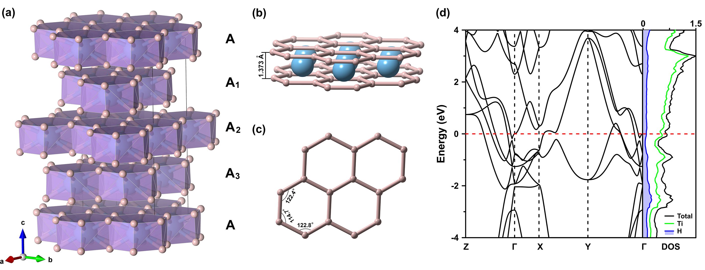
Figure 5: (Color online) (a) Polyhedral representation of the Fddd-TiH₄ structure. Ti-centered hexagonal prisms are shown in purple. (b) The fundamental “sandwich” of TiH₄. (c) Distorted H-graphene layer in Fddd-TiH₄, and (d) electronic band structure and density of states (DOS) of Fddd-TiH₄ at 300 GPa; DOS is in the unit of states/formula/eV and Fermi energy (red dashed line) is set to zero.

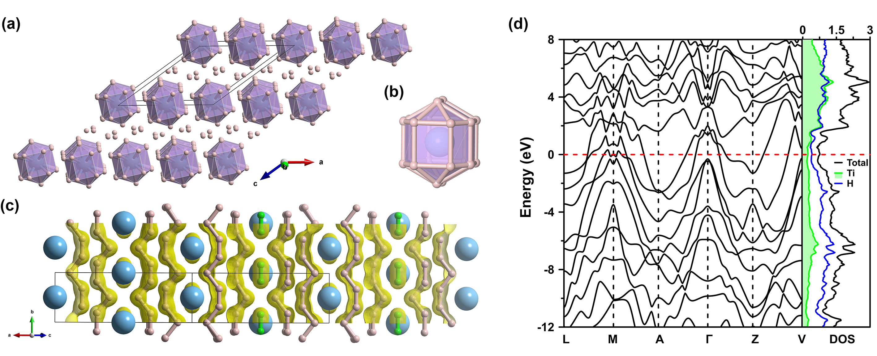
Figure 6: (Color online) (a) Polyhedral representation of the C2/m-TiH₂₂ structure. (b) Expanded view of a H₂₀ cage encapsulating a Ti atom. (c) ELF isosurface (ELF=0.7) for C2/m-TiH₂₂ at 350 GPa. Green and pink atoms represent molecular hydrogen and armchair-like hydrogen chains, respectively. (d) Electronic band structure and DOS for C2/m-TiH₂₂ at 350 GPa.

The most interesting part is that besides hydrogen-rich TiH₁₄ stoichiometry, an extremely H-rich structure TiH₂₂ is identified to be thermodynamically stable in a monoclinic structure at pressures above 235 GPa. To the best of our knowledge, C2/m-TiH₂₂ presently is the second hydrogen-richest hydrides known or predicted to date, after metal hydride C2/c-YH₂₄Peng et al. (2017). The polyhedral crystal structure representation of C2/m-TiH₂₂ [depicted in Fig. 6(a)] exhibits alternations of H₂ molecules and TiH₂₀ polyhedra. Titanium is encapsulated in H₂₀ cages with Ti-H distances are 1.62–1.66 Å at 350 GPa, as shown in Fig. 6(b). The band structure and density of states (DOS) of C2/m-TiH₂₂ at 350 GPa [Fig. 6(d)] indicate metallicity of TiH₂₂. The total DOS of C2/m-TiH₂₂ near the Fermi level N($\varepsilon_{F}$) mostly comes from H atoms, which is opposite to Fddd-TiH₄ [Fig. 5(d)]. The coexistence of molecular hydrogen with an H–H distance of 0.819 Å and armchair-like hydrogen chain is clearly revealed by the electron localization function (ELF). As shown in ELF Fig. 6(c), the regions with ELF values of 0.7 include H₂ molecules and armchair-like hydrogen chain, which indicates strong covalent bonding between hydrogen atoms.

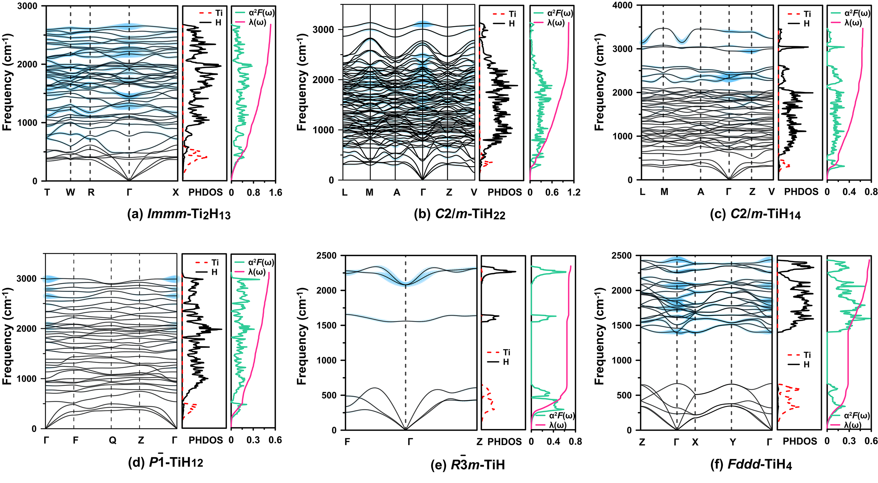
Figure 7: (Color online) Phonon dispersion curves, phonon density of states projected onto selected atoms, Eliashberg spectral function $\alpha^{2}\emph{F}(\omega)$, and the electron–phonon coupling (EPC) parameter $\lambda$ for (a) Immm-Ti₂H₁₃ at 350 GPa, (b) C2/m-TiH₂₂ at 250 GPa, (c) C2/m-TiH₁₄ at 200 GPa, (d) P$\bar{1}$-TiH₁₂ at 350 GPa, (e) R$\bar{3}$m-TiH at 200 GPa and (f) Fddd-TiH₄ at 350 GPa. The magnitude of the phonon linewidths is indicated by the size of the blue open circles with the radius proportional to the respective coupling strength.

Based on the calculated phonon dispersion spectrum at high pressure [displayed in Fig.7 and Fig. S1], no imaginary vibrational frequencies are found in the whole Brillouin zone, indicating the dynamical stability of all the predicted structures. Phonon dispersion curves, phonon density of states, phonon linewidths $\gamma_{\mathbf{q}\nu}$, Eliashberg phonon spectral function $\alpha^{2}F(\omega)$, and the electron-phonon coupling parameter $\lambda$ of Immm-Ti₂H₁₃ , C2/m-TiH₂₂ , I$\bar{4}$-Ti₅H₁₄, P$\bar{1}$-TiH₁₂, R$\bar{3}$m-TiH and Fddd-TiH₄, at selected pressures are depicted in Fig.7. As expected (due to atomic masses), low-frequency modes are mostly related to Ti atoms whereas high-frequency modes are dominated by vibrations of H ones. Moreover, in all of these six structures, the $\gamma_{\mathbf{q}\nu}$ of branches near the $\Gamma$ point are much greater than those elsewhere in the Brillouin zone. The total $\lambda$ of R$\bar{3}$m-TiH is mainly contributed by the acoustic modes, whereas those of the other five structures are dominated by optical branches.

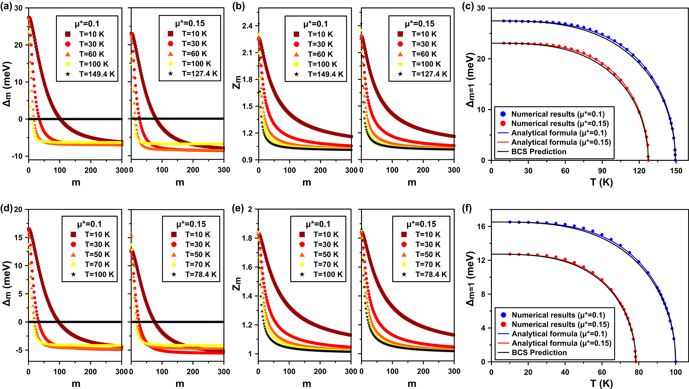
Figure 8: (Color online) Dependence of the superconducting order parameter on the number m for select values of temperature and Coulomb pseudopotential for (a) Immm-Ti₂H₁₃ at 350 GPa and (d) C2/m-TiH₂₂ at 250 GPa. The wave function renormalization factor Z${}_{\text{m}}$ on the imaginary axis for select values of temperature and Coulomb pseudopotential for (b) Immm-Ti₂H₁₃ and (e) C2/m-TiH₂₂. The influence of temperature on the maximum value of the order parameter ($\Delta_{m=1}$) for selected $\mu$^∗ of (c) Immm-Ti₂H₁₃ and (f) C2/m-TiH₂₂. Solid circles correspond to the exact numerical solutions of the Eliashberg equations, the red and blue lines represent the results obtained using analytical formulas [Eq.10]. Black lines are predicted by BCS model [Eq.10, where $\Gamma$=3]

We further probe superconductivity of these hydrides, using BCS theory. The calculated superconducting properties are summarized in Table 1. All of the predicted titanium hydrides exhibit superconductivity at high pressures. The highest T_c of titanium hydrides are possessed by Immm-Ti₂H₁₃, C2/m-TiH₂₂, I$\bar{4}$-Ti₅H₁₄, P$\bar{1}$-TiH₁₂, R$\bar{3}$m-TiH and Fddd-TiH₄. I4/mmm-TiH₂ exhibits low T_c values (3 mK, $\mu^{*}$=0.1) at 50 GPa. On the other hand, superconductivity of titanium monohydride (TiH) comes largely from strong coupling of the electrons with Ti vibrations, and coupling with H vibrations becomes more important as H content increases. Intriguingly, it is Immm-Ti₂H₁₃ instead of C2/m-TiH₂₂ that possesses the highest T_c among searched titanium hydrides. The results from the previous studiesLiu et al. (2017); Zhong et al. (2016) suggest higher hydrogen content in the binary hydrides is one of the necessary prerequisites to obtain higher T_c value. This is not necessarily always the case; the hydrogen content in C2/m-TiH₂₂ is much higher than in Immm-Ti₂H₁₃. Indeed, $\omega_{\textit{log}}$ of C2/m-TiH₂₂ is larger than that of Immm-Ti₂H₁₃. However, this is offset by the lower $\lambda$ of C2/m-TiH₂₂ ($\lambda$=0.861) compared with that of Immm-Ti₂H₁₃ ($\lambda$=1.423). The $\alpha^{2}F(\omega)$ was used for numerically solving the Eliashberg equations and the obtained T_c of Immm-Ti₂H₁₃ is in the range 110.4–131.2 K ($\lambda$=1.423, $\mu^{*}$=0.1–0.15) at 350 GPa.

Table 1: The EPC parameter $\lambda$, electronic density of states at Fermi level N($\varepsilon_{F}$) (states/Ry/cell), the logarithmic average phonon frequency $\omega_{log}$ (K) and superconducting critical temperatures T_c (K) for titanium hydrides at different pressure P (GPa). T_c values are given for $\mu^{*}$=0.1 and T_c in brackets are for $\mu$=0.15; T_c (McM) is the numerical solution of solving the imaginary axis Eliashberg equation, T_c (A–D) is calculated from the Allen–Dynes equation and T_c (E) is obtained by Allen–Dynes modified McMillan equation.

Compound	P	$\lambda$	N($\varepsilon_{F}$)	$\omega_{log}$	Tc (McM)	Tc (A–D)	Tc (E)
C2/m-TiH22	350	0.861	4.765	1677.4	90.7 (65.0)	93.6 (67.3)	100.0 (78.4)
	250	1.057	4.867	1296.2	98.1 (76.7)	103.1 (80.7)	110.2 (91.3)
C2/m-TiH14	200	0.645	5.243	1201.7	33.9 (19.7)	35.0 (20.3)	35.9 (25.0)
P$\bar{1}$-TiH12	350	0.514	3.213	1357.6	18.4 (7.8)	18.8 (8.0)	19.5 (11.5)
	150	0.403	3.748	1074.8	4.7 (1.0)	4.8 (1.0)	5.4 (2.4)
Immm-Ti2H13	350	1.423	10.028	1101.3	119.3 (100.8)	131.2 (110.4)	149.4 (127.4)
Fddd-TiH4	350	0.574	3.803	1034.4	20.6 (10.4)	21.2 (10.7)	20.1 (6.2)
Fm$\bar{3}$m-TiH3	100	0.528	6.798	459.4	6.9 (3.1)	7.1 (3.1)	7.5 (4.7)
I$\bar{4}$-Ti5H14	350	0.411	20.738	479.9	2.4 (0.6)	2.4 (0.6)	2.8 (1.4)
	50	0.477	35.785	525.6	5.3 (1.9)	5.4 (2.0)	5.8 (3.3)
I4/m-Ti5H13	300	0.470	22.211	412.6	3.9 (1.4)	4.0 (1.4)	4.4 (2.7)
	150	0.406	27.253	450.8	2.1 (0.5)	2.1 (0.5)	2.5 (1.1)
Ibam-Ti2H5	250	0.504	9.910	363.3	4.6 (1.9)	4.7 (1.9)	5.1 (3.2)
	50	0.564	12.852	365.0	6.9 (3.4)	7.1 (3.5)	6.9 (4.6)
Cmma-TiH2	250	0.509	3.604	434.3	5.7 (2.4)	5.8 (2.4)	6.0 (3.7)
I4/mmm-TiH2	50	0.227	3.687	0.0 (0.0)	0.0 (0.0)	0.0 (0.0)	0.0 (0.0)
R$\bar{3}$m-TiH	350	0.714	4.328	597.3	21.8 (13.9)	22.7 (14.4)	23.9 (18.2)
I4/mmm-TiH	200	0.991	6.303	264.3	18.1 (13.8)	19.5 (14.8)	22.5 (18.9)
	50	1.013	8.716	71.0	5.0 (3.9)	5.4 (4.1)	12.6 (10.0)

For Immm-Ti₂H₁₃ at 350 GPa and C2/m-TiH₂₂ at 250 GPa, the dependence of the maximum value of the order parameter on temperature for selected $\mu^{*}$ is presented in Fig. 8(c) and (f). The maximum value of order parameter $\Delta_{m=1}$ decreases with the growth of T and $\mu^{*}$. On the basis of these results, $\Delta_{m=1}$ value can be characterized analytically by means of the phenomenological formula

$${\textstyle\Delta_{m=1}(T,\mu^{*})=\Delta_{m=1}(T_{0},\mu^{*})\sqrt{1-\left(\frac{T}{T_{c}}\right)^{\Gamma}}}.$$ (10)

For the maximum value of order parameter $\Delta_{m=1}$, we obtained the estimation of temperature exponent for Immm-Ti₂H₁₃ ($\Gamma$=3.25 for $\mu^{*}$=0.1; $\Gamma$=3.31 for $\mu^{*}$=0.15) and C2/m-TiH₂₂ ($\Gamma$=3.21 for $\mu^{*}$=0.1; $\Gamma$=3.16 for $\mu^{*}$=0.15). It is clear that the temperature dependence of maximum order parameter obtained in Eliashberg equations only differs a little bit from the results estimated by the BCS theory, where $\Gamma$=3 (Ref. Eschrig, 2001). It can be seen that the values of order parameter strongly decrease together with the increase of the Coulomb pseudopotential [Fig. 8(a) and (d)]. On the other hand, the influence of the Coulomb pseudopotential $\mu^{*}$ on the wavefunction renormalization factor [Fig. 8(b) and (e)] is significantly weaker. Through comparison among above three approaches of calculating T_c, it can be seen that two analytical results generally underestimate T_c, especially for the high values of the Coulomb pseudopotential. Moreover, the Allen–Dynes formula much better reproduces the numerical results than the modified McMillan expression. Note that anharmonicity, which usually decreases T_c, is not included in our calculations.

The influence of pressure on T_c has been widely discussed before. Theoretical studies of some systemsYu et al. (2015); Liu et al. (2017); Kvashnin et al. (2018) show that T_c will decrease with increasing pressure; someKim et al. (2010); Li et al. (2014) report T_c to increase with pressure; and othersZhang et al. (2015); Zheng et al. (2018) reveal negligible pressure dependence. The first two situations can be reflected in Ti–H system. For example, the T_c of C2/m-TiH₂₂, I$\bar{4}$-Ti₅H₁₄, Ibam-Ti₂H₅ and I4/mmm-TiH decrease with pressure, whereas T_c of P$\bar{1}$-TiH₁₂ and I4/m-Ti₅H₁₃ increase. One of the important factors explaining the effect of pressure on T_c is related to phonon softening. In case of C2/m-TiH₂₂, phonon modes around the A and Z points harden with pressure [see Figs. 7(b) and S1(a)]. The same tendency can also be seen around the P and N points in the Brillouin zone of I$\bar{4}$-Ti₅H₁₄ on increasing pressure. For P$\bar{1}$-TiH₁₂, phonon modes around the $\Gamma$ and Z point soften with pressure. This means that phonon modes around high-symmetry points harden with pressure, leading to a decrease of the value of T_c. On the contrary, phonon softening with pressure gives rise to the increase of T_c.

IV Conclusions

In order to discover high-T_c superconductors, the Ti–H system at pressures up to 350 GPa was systematically explored using the ab initio evolutionary algorithm USPEX. A phase (R$\bar{3}$m-TiH) and several stoichiometries (C2/m-TiH₂₂, P$\bar{1}$-TiH₁₂, Immm-Ti₂H₁₃, Fddd-TiH₄, I$\bar{4}$-Ti₅H₁₄, I4/m-Ti₅H₁₃ and Ibam-Ti₂H₅) were predicted, and found to be dynamically stable in their predicted pressure ranges of stability. With increasing pressure, I4/mmm-TiH transforms into R$\bar{3}$m-TiH at 230 GPa, and I4/mmm-TiH₂ into Cmma-TiH₂ at 78 GPa. Cmma-TiH₂ is structurally similar to P4/nmm-TiH₂. C2/m-TiH₂₂ has the highest hydrogen content among all titanium hydrides, and contains TiH₂₀ cages. The estimated T_c of Immm-Ti₂H₁₃ is 127.4–149.4 K ($\mu^{*}$=0.1–0.15) at 350 GPa, which is actually higher than T_c of the aforementioned C2/m-TiH₂₂ of 91.3–110.2 K at 250 GPa. Superconductivity of Immm-Ti₂H₁₃ mainly arises from both strong coupling of the electrons with H vibrations and the large logarithmic average phonon frequency. The accuracy of three methods for estimating the T_c were compared. Taking solution of the Eliashberg equations as standard, the estimated T_c from Allen–Dynes formula is more accurate than that from the modified McMillan expression. The constructed pressure–composition phase diagram and the analysis of superconductivity of titanium hydrides will motivate future experimental synthesis of titanium hydrides and studies of their high-temperature superconductivity.

V acknowledgments

J. M. M. acknowledges startup support from Washington State University and the Department of Physics and Astronomy thereat. A. R. O. thanks Russian Science Foundation (grant 19-72-30043) for financial support.

References

- Ginzburg (1999) V. L. Ginzburg, Phys.-Uspekhi 42, 353 (1999).
- Van Delft and Kes (2010) D. Van Delft and P. Kes, Phys. Today 63, 38 (2010).
- Duan et al. (2014) D. Duan, Y. Liu, F. Tian, D. Li, X. Huang, Z. Zhao, H. Yu, B. Liu, W. Tian, and T. Cui, Sci. Rep. 4, 6968 (2014).
- Drozdov et al. (2015) A. Drozdov, M. Eremets, I. Troyan, V. Ksenofontov, and S. Shylin, Nature 525, 73 (2015).
- Liu et al. (2017) H. Liu, I. I. Naumov, R. Hoffmann, N. Ashcroft, and R. J. Hemley, Proc. Natl. Acad. Sci. 114, 6990 (2017).
- Bi et al. (2019) T. Bi, N. Zarifi, T. Terpstra, and E. Zurek, Reference Module in Chemistry, Molecular Sciences and Chemical Engineering (2019).
- Somayazulu et al. (2019) M. Somayazulu, M. Ahart, A. K. Mishra, Z. M. Geballe, M. Baldini, Y. Meng, V. V. Struzhkin, and R. J. Hemley, Phys. Rev. Lett. 122, 027001 (2019).
- Drozdov et al. (2019) A. Drozdov, P. Kong, V. Minkov, S. Besedin, M. Kuzovnikov, S. Mozaffari, L. Balicas, F. Balakirev, D. Graf, V. Prakapenka, et al., Nature 569, 528 (2019).
- Lorenz and Chu (2005) B. Lorenz and C. Chu, in Frontiers in Superconducting Materials (Springer, 2005) pp. 459–497.
- Gao et al. (1994) L. Gao, Y. Xue, F. Chen, Q. Xiong, R. Meng, D. Ramirez, C. Chu, J. Eggert, and H. Mao, Phys. Rev. B 50, 4260 (1994).
- Ashcroft (1968) N. W. Ashcroft, Phys. Rev. Lett. 21, 1748 (1968).
- Ashcroft (2004a) N. W. Ashcroft, Phys. Rev. Lett. 92, 187002 (2004a).
- Ashcroft (2004b) N. W. Ashcroft, J. Phys. Condens. Matter 16, S945 (2004b).
- Xie et al. (2014) Y. Xie, Q. Li, A. R. Oganov, and H. Wang, Acta Crystallogr. C 70, 104 (2014).
- Feng et al. (2015) X. Feng, J. Zhang, G. Gao, H. Liu, and H. Wang, RSC Adv. 5, 59292 (2015).
- Wang et al. (2012) H. Wang, S. T. John, K. Tanaka, T. Iitaka, and Y. Ma, Proc. Natl. Acad. Sci. 109, 6463 (2012).
- Abe (2017) K. Abe, Phys. Rev. B 96, 144108 (2017).
- Li et al. (2017) X.-F. Li, Z.-Y. Hu, and B. Huang, Phys. Chem. Chem. Phys. 19, 3538 (2017).
- Liu et al. (2015) Y. Liu, X. Huang, D. Duan, F. Tian, H. Liu, D. Li, Z. Zhao, X. Sha, H. Yu, H. Zhang, et al., Sci. Rep. 5, 11381 (2015).
- Zhuang et al. (2017) Q. Zhuang, X. Jin, T. Cui, Y. Ma, Q. Lv, Y. Li, H. Zhang, X. Meng, and K. Bao, Inorg. Chem. 56, 3901 (2017).
- Gao et al. (2010) G. Gao, A. R. Oganov, P. Li, Z. Li, H. Wang, T. Cui, Y. Ma, A. Bergara, A. O. Lyakhov, T. Iitaka, et al., Proc. Natl. Acad. Sci. 107, 1317 (2010).
- Kruglov et al. (2018) I. A. Kruglov, D. V. Semenok, H. Song, , I. A. Wrona, R. Akashi, M. Esfahani, D. Duan, T. Cui, A. G. Kvashnin, and A. R. Oganov, arXiv preprint arXiv:1810.01113 (2018).
- Esfahani et al. (2016) M. M. D. Esfahani, Z. Wang, A. R. Oganov, H. Dong, Q. Zhu, S. Wang, M. S. Rakitin, and X.-F. Zhou, Sci. Rep. 6, 22873 (2016).
- Flores-Livas et al. (2016) J. A. Flores-Livas, A. Sanna, and E. Gross, Eur. Phys. J. B 89, 63 (2016).
- Zhong et al. (2016) X. Zhong, H. Wang, J. Zhang, H. Liu, S. Zhang, H.-F. Song, G. Yang, L. Zhang, and Y. Ma, Phys. Rev. Lett. 116, 057002 (2016).
- Semenok et al. (2018) D. V. Semenok, I. A. Kruglov, A. G. Kvashnin, and A. R. Oganov, arXiv preprint arXiv:1806.00865 (2018).
- Yakel (1958) H. Yakel, Acta Crystallogr. 11, 46 (1958).
- San-Martin and Manchester (1987) A. San-Martin and F. Manchester, Bull. Alloy Phase Diagr. 8, 30 (1987).
- Vennila et al. (2008) R. S. Vennila, A. Durygin, M. Merlini, Z. Wang, and S. Saxena, Int. J. Hydrog. Energy 33, 6667 (2008).
- Kalita et al. (2010) P. E. Kalita, S. V. Sinogeikin, K. Lipinska-Kalita, T. Hartmann, X. Ke, C. Chen, and A. Cornelius, J. Appl. Phys. 108, 043511 (2010).
- Endo et al. (2013) N. Endo, H. Saitoh, A. Machida, Y. Katayama, and K. Aoki, J. Alloys Compd. 546, 270 (2013).
- Shanavas et al. (2016) K. V. Shanavas, L. Lindsay, and D. S. Parker, Sci. Rep. 6, 28102 (2016).
- Oganov and Glass (2006) A. R. Oganov and C. W. Glass, J. Chem. Phys. 124, 244704 (2006).
- Oganov et al. (2011) A. R. Oganov, A. O. Lyakhov, and M. Valle, Acc. Chem. Res. 44, 227 (2011).
- Lyakhov et al. (2013) A. O. Lyakhov, A. R. Oganov, H. T. Stokes, and Q. Zhu, Comput. Phys. Commun. 184, 1172 (2013).
- Perdew et al. (1996) J. P. Perdew, K. Burke, and M. Ernzerhof, Phys. Rev. Lett. 77, 3865 (1996).
- Kresse and Furthmüller (1996) G. Kresse and J. Furthmüller, Phys. Rev. B 54, 11169 (1996).
- Blöchl (1994) P. E. Blöchl, Phys. Rev. B 50, 17953 (1994).
- Kresse and Joubert (1999) G. Kresse and D. Joubert, Phys. Rev. B 59, 1758 (1999).
- Togo et al. (2008) A. Togo, F. Oba, and I. Tanaka, Phys. Rev. B 78, 134106 (2008).
- Baroni et al. (2001) S. Baroni, S. De Gironcoli, A. Dal Corso, and P. Giannozzi, Rev. Mod. Phys. 73, 515 (2001).
- Giannozzi et al. (2009) P. Giannozzi, S. Baroni, N. Bonini, M. Calandra, R. Car, C. Cavazzoni, D. Ceresoli, G. L. Chiarotti, M. Cococcioni, I. Dabo, et al., J. Phys. Condens. Matter 21, 395502 (2009).
- Giannozzi et al. (2017) P. Giannozzi, O. Andreussi, T. Brumme, O. Bunau, M. B. Nardelli, M. Calandra, R. Car, C. Cavazzoni, D. Ceresoli, M. Cococcioni, N. Colonna, I. Carnimeo, A. D. Corso, S. de Gironcoli, P. Delugas, R. A. D. Jr, A. Ferretti, A. Floris, G. Fratesi, G. Fugallo, R. Gebauer, U. Gerstmann, F. Giustino, T. Gorni, J. Jia, M. Kawamura, H.-Y. Ko, A. Kokalj, E. Küçükbenli, M. Lazzeri, M. Marsili, N. Marzari, F. Mauri, N. L. Nguyen, H.-V. Nguyen, A. O. de-la Roza, L. Paulatto, S. Poncé, D. Rocca, R. Sabatini, B. Santra, M. Schlipf, A. P. Seitsonen, A. Smogunov, I. Timrov, T. Thonhauser, P. Umari, N. Vast, X. Wu, and S. Baroni, J. Phys. Condens. Matter 29, 465901 (2017).
- Grimaldi et al. (1999) C. Grimaldi, L. Pietronero, and M. Scattoni, Eur. Phys. J. B 10, 247 (1999).
- Migdal (1958) A. Migdal, Sov. Phys. JETP 7, 996 (1958).
- Allen and Mitrović (1983) P. B. Allen and B. Mitrović, in Phys. Status Solidi, Vol. 37 (Elsevier, 1983) pp. 1–92.
- Szczesniak (2006) R. Szczesniak, Acta Phys. Pol. A 109, 179 (2006).
- Szcze et al. (2012) R. Szcze, D. Szcze, E. Drzazga, et al., Solid State Commun. 152, 2023 (2012).
- Chan et al. (2012) K. T. Chan, B. D. Malone, and M. L. Cohen, Phys. Rev. B 86, 094515 (2012).
- Chase (1998) M. W. Chase, NIST-JANAF Thermochemical Tables 2 Volume-Set (Journal of Physical and Chemical Reference Data Monographs), Vol. 2 (Wiley New York, 1998).
- Zhuang et al. (2018) Q. Zhuang, X. Jin, T. Cui, D. Zhang, Y. Li, X. Li, K. Bao, and B. Liu, Phys. Rev. B 98, 024514 (2018).
- Peng et al. (2017) F. Peng, Y. Sun, C. J. Pickard, R. J. Needs, Q. Wu, and Y. Ma, Phys. Rev. Lett. 119, 107001 (2017).
- Eschrig (2001) H. Eschrig, (2001).
- Yu et al. (2015) S. Yu, X. Jia, G. Frapper, D. Li, A. R. Oganov, Q. Zeng, and L. Zhang, Sci. Rep. 5, 17764 (2015).
- Kvashnin et al. (2018) A. G. Kvashnin, D. V. Semenok, I. A. Kruglov, I. A. Wrona, and A. R. Oganov, ACS Appl. Mater. Interfaces 10, 43809 (2018).
- Kim et al. (2010) D. Y. Kim, R. H. Scheicher, H.-k. Mao, T. W. Kang, and R. Ahuja, Proc. Natl. Acad. Sci. 107, 2793 (2010).
- Li et al. (2014) Y. Li, J. Hao, H. Liu, Y. Li, and Y. Ma, J. Chem. Phys. 140, 174712 (2014).
- Zhang et al. (2015) S. Zhang, Y. Wang, J. Zhang, H. Liu, X. Zhong, H.-F. Song, G. Yang, L. Zhang, and Y. Ma, Sci. Rep. 5, 15433 (2015).
- Zheng et al. (2018) S. Zheng, S. Zhang, Y. Sun, J. Zhang, J. Lin, G. Yang, and A. Bergara, Front. Phys. 6, 101 (2018).