Pumping Patterns and Work Done during Peristalsis in Finite-length Elastic Tubes

Abstract

Balloon dilation catheters are often used to quantify the physiological state of peristaltic activity in tubular organs and comment on their ability to propel fluid which is important for healthy human function. To fully understand this system’s behavior, we analyzed the effect of a solitary peristaltic wave on a fluid-filled elastic tube with closed ends. A reduced order model that predicts the resulting tube wall deformations, flow velocities and pressure variations is presented. This simplified model is compared with detailed fluid-structure 3D immersed boundary simulations of peristaltic pumping in tube walls made of hyperelastic material. The major dynamics observed in the 3D simulations were also displayed by our 1D model under laminar flow conditions. Using the 1D model, several pumping regimes were investigated and presented in the form of a regime map that summarizes the system’s response for a range of physiological conditions. Finally, the amount of work done during a peristaltic event in this configuration was defined and quantified. The variation of elastic energy and work done during pumping was found to have a unique signature for each regime. An extension of the 1D model is applied to enhance patient data collected by the device and find the work done for a typical esophageal peristaltic wave. This detailed characterization of the system’s behavior aids in better interpreting the clinical data obtained from dilation catheters. Additionally, the pumping capacity of the esophagus can be quantified for comparative studies between disease groups.

Keywords: esophagus, elastic tube flow, peristalsis, reduced-order modeling, fluid-structure interaction, immersed boundary method

1 Introduction

Peristaltic flow through cylinders and other geometries has been studied extensively since the mid 1960s [1, 2, 3, 4]. The investigations have ranged from analyses of specified wall motion on Newtonian [5, 1], non-Newtonian [6, 7] and particulate fluids [8, 9, 10] to the effects of a prescribed forcing on the coupled fluid-structure system [11, 12, 13]. Both infinite and finite geometries [14, 13] have been considered and the quantitative effects of the channel geometry (cylindrical vs. rectangular channels) on pumping characteristics have been established [3, 15]. However, one problem that has received little attention is the effect of peristalsis on fluid-filled elastic tubes that are closed at both ends. In such a setting, fluid inside the tube can neither enter nor leave the system for the entire duration of peristalsis. This configuration is commonly found in long, slender balloon catheters used to evaluate mechanical properties and the contractile response of blood vessels (similar to catheters used during angioplasty). It is also found in functional lumen imaging probe (FLIP) catheters used to characterize the contractility of anatomical sphincters and esophageal motility.

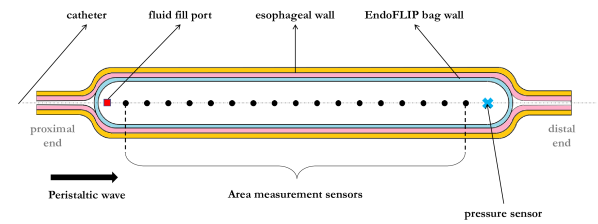
Figure 1: Details of the FLIP bag and catheter assembly (positioned within the esophagus). The proximal end of the bag points towards the subject’s throat and the distal end, towards the stomach. The length of the bag is 16 cm and diameter at full distension is 22 mm.

A major assumption utilized to facilitate the mathematical analysis of peristaltic flow through a tube is that the problem is identical in both the fixed (lab) frame of reference and in the reference frame attached to the peristaltic wave. In the latter, the wave is stationary and the shape of the tube walls does not change with time. When the tube length is finite, this assumption is not valid [14]. Thus, in order to build a simplified model for our problem, we turn to the approach taken to analyze flow driven by valveless pumping, which occurs in a finite, periodic domain, and modify the forcing method and boundary conditions to reflect the operating conditions for our problem. Interestingly, the configuration we aim to study first appears in [1], but is subsequently ignored. To the best of our knowledge, this configuration does not appear again in any other studies involving flow in deformable tubes.

The device we intend to focus our analysis on is the aforementioned FLIP [16]. It consists of a long flexible, hollow catheter, at the end of which is mounted a polyurethane bag [17]. The section of the catheter enclosed by the bag incorporates paired impedance planimetry sensors that can measure the regional cross-sectional area (CSA) along the bag’s length as seen in Fig. 1. Various versions of the device exist where the bag length is either 8 or 16 cm; our focus is on the latter version. Also within the bag at the distal end is a pressure sensor that captures the fluid pressure at any given time. When deployed in a patient, the device is positioned such that most of the bag rests within the esophageal lumen. The bag is then incrementally filled with saline and the esophageal contractile response is evaluated by monitoring the internal fluid pressure and CSAs along the length of the bag. When fully distended with saline, the bag diameter is 22 mm. The external end of the catheter is connected to a computer that stores the data collected by these sensors. The bag can be filled or drained by pumping fluid through the catheter and fluid enters or leaves the bag through a small hole on the catheter. Figure 1 shows a simplified representation of the bag-catheter assembly and shows the locations of the various sensors. For additional details on the device’s construction, data resolution, accuracy and frequency of data collection, see Refs. [16] and [18].

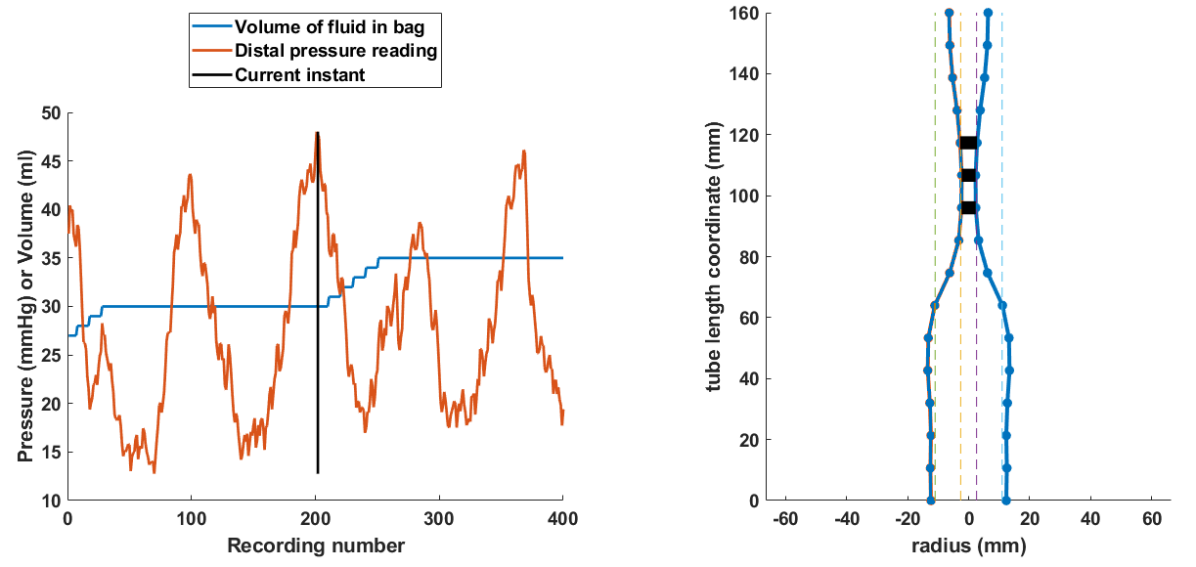
Figure 2: Visualization of clinical data collected from the FLIP. Graph on the left shows the bag volume and pressure variation over 40 seconds of time (10 Hz recording frequency). Figure on the right shows the profile of the esophageal lumen at the instant marked by the vertical black bar on the left graph (at recording number 200). Dotted lines show the range of measurable cross-sectional area (21 - 380 $\mathrm{mm}^{2}$, 5.2 - 22 mm diameter) [16].

1.1 Operating Details and Simplifying Assumptions

Representative FLIP data obtained from a subject can be visualized as shown in Fig. 2. During examination, the subject is in a supine position. The left panel shows the pressure and volume inside the bag as a function of time. It should be noted that the volume change is controlled by the physician conducting the procedure and that the pressure change is a consequence of esophageal contractility in response to distension. The right panel of the figure shows the axisymmetric profile of the tube at the instant in time indicated by the black vertical line on the left panel. The dotted lines superimposed on the tube profile show the maximum and minimum diameters that can be accurately measured by the planimetry sensors. The esophageal contraction is highlighted with the three black bands where the CSA is the least. On the pressure curve, we see four peaks indicating that four peristaltic waves have passed over the bag for the duration of this plot. The image of the bag profile is oriented such that peristalsis begins at the top and travels downward. Measurement of area is not continuous along the bag’s length. Rather, area is measured at 16 locations at 1 cm intervals and intermediate values are interpolated to construct the lumen profile [19].

With the device located in the esophagus, the passage of a peristaltic wave causes the (axisymmetric) profile of the bag and fluid pressure within it to change. During peristalsis, the esophageal wall may or may not approximate (i.e. come in contact with) the catheter. It is difficult to predict the relationship between flow rate and pressure drop across the contraction zone. The Reynolds number ($Re$) of the system is estimated to be 660 when using the following values: density $\rho=1000\ \text{kg/m}^{3}$, viscosity $\mu=0.001\ \text{Pa}\cdot\text{s}$, tube diameter $D=22\ \text{mm}$ and peristaltic wave speed $c=3\ \text{cm/s}$ [20]. If the flow inside is assumed to be similar to pipe flow at every location, then the flow is laminar. But the Reynolds number in the contraction zone is difficult to estimate so the nature of flow at the neck is unknown. As such, we will analyze two flow types, (corresponding to low and high $Re$): 1) parabolic flow everywhere and 2) assuming that that a simple friction factor can be used to relate flow rate and pressure drop in the entire domain. As the subject is in a supine position, we assumed that the effect of gravity on the device is negligible. Depending on the positioning of the esophagus in the subject, the catheter can become slightly curved during measurement. The impedance planimetry sensors measure only local lumen area. Thus, curvature information is not available during clinical examination or subsequent analysis. However, fluoroscopic imaging [21] shows that the curvature is not significant, thus we assume a straight geometry to model this problem. During the procedure, bag volume is changed from 0 to 70 mL in 10 mL steps. The analysis presented in this work considers peristaltic activity occurring at 30 or 40 mL of distension where the esophagus is gently stretched and circumferential wall strains are not high. Due to the inflated nature of the bag, the lumen profile tends to be largely circular.

Our goal was to build a simple model to analyze this system and understand the relationships between the tube profile, internal bag pressure, esophageal wall stiffness and the intensity of the peristaltic contraction. With sound mathematical foundations, the work done by the esophageal walls to pump fluid within the bag can be defined. This fast, simple model will eventually be deployed at point-of-care to estimate pressure distributions and work done in real time. Armed with this knowledge, we can quantify peristaltic work of the esophagus, which may prove valuable in the evaluation of dysphagia.

2 Mathematical Details of the 1-D Model

Incompressible flow in a tube with deforming walls can be modeled using the system of equations given by (1) and (2). Here, $A(x,t)$ is the tube area and $u(x,t)$ is the area-averaged fluid velocity in the axial direction. The axial coordinate along the tube length is denoted by $x$ and time by $t$. Equation (1) is the continuity equation that relates local changes in tube area and fluid velocity to conserve volume. Equation (2) describes the conservation of momentum with a general flow resistance term $2\tau_{R}/(\rho R)$ due to fluid viscosity and a momentum correction factor of unity [22]. These equations have been widely used to describe valveless pumping [23, 24], and a detailed derivation of these equations can be found in [25].

$$\frac{\partial A}{\partial t}+\frac{\partial\left(Au\right)}{\partial x}=0$$ (1)

$$\frac{\partial u}{\partial t}+u\frac{\partial u}{\partial x}=-\frac{1}{\rho}\frac{\partial p}{\partial x}-\frac{2\tau_{R}}{\rho R}.$$ (2)

In the context of peristalsis-driven flow in the esophagus, fluid velocities are much smaller than the velocity at which a disturbance propagates in the esophageal wall. Thus, we expect no shocks or discontinuities in the problem which allows us to use the non-conservative forms of the continuity and momentum equations. For smooth solutions, both conservative and non-conservative versions of the governing equations are equivalent and will lead to the same numerical solution.

To close the system of equations, we assume that a constitutive law in the form of an explicit relationship between pressure $p$ and area $A$ exists. This relationship is commonly referred to as a “tube law”. For our application, we assume that the change in pressure is proportional to the change in area. Experiments carried out with the FLIP show that the distal esophageal walls follow this behavior [26] and a similar form of the tube law is also used in [24] and derived in [27] using shell theory. The external pressure is assumed to be zero for all time and thus the transmural pressure is equal to the pressure inside the tube. A damping term is introduced to regularize the system of equations. The form of the tube law used is given by

$$p=K\left(\frac{A}{\theta A_{0}}-1\right)+Y\frac{\partial A}{\partial t}.$$ (3)

Here, $K$ is a measure of the wall stiffness and has the units of pressure. Its exact value depends on the Young’s modulus of the muscle wall and the ratio of its thickness to the undeformed radius. The tube’s undeformed, reference area $A_{0}$, is changed by an activation factor $\theta=\theta(x,t)$ to introduce the effect of a contraction. A damping term with coefficient $Y$ is also introduced. By a simple manipulation using the continuity equation, we can see that the introduction of this term leads to a diffusion term in the momentum equation:

$$p=K\left(\frac{A}{\theta A_{0}}-1\right)+Y\frac{\partial A}{\partial t}=K\left(\frac{A}{\theta A_{0}}-1\right)-Y\frac{\partial\left(Au\right)}{\partial x}$$ (4)

$$\frac{\partial p}{\partial x}=\frac{K}{A_{0}}\frac{\partial}{\partial x}\left(\frac{A}{\theta}\right)-Y\frac{\partial^{2}\left(Au\right)}{\partial x^{2}}.$$ (5)

Thus, the addition of this term helps stabilize the numerical solution. A similar manipulation was also used in [22] to eliminate $p$. In our analysis, the damping is kept small so as to ensure that the linear part of the tube law is the major contributor to fluid pressure for all regimes of operation. Note that $A(x,t)$ and $\theta A_{0}$ are not equal. The former is an unknown whose value must be found as part of the solution. Before proceeding, it is important to make note of the viscous shear stress term in the momentum equation. Several approximations can be made to write $\tau_{R}$ as a function of tube area and local fluid velocity. For our analysis, we choose to study the system when 1) the flow is parabolic everywhere with viscosity $\mu$ and, 2) a viscous term that uses a constant friction factor $f$ is used to compute flow stresses. In the former case, the viscous resistance term $2\tau_{R}/(\rho R)$ is equal to $8\pi\mu u/(\rho A)$ and is $fu|u|/(2D)$ for the latter.

2.1 Non-dimensional Version of the Governing Equations

The following expressions were chosen for each of the dimensional variables to obtain non-dimensional versions of the continuity, momentum and the tube law equations:

$$A=\alpha A_{0},\qquad t=\tau\frac{L}{c},\qquad u=Uc,$$ (6)

$$p=PK\qquad\text{and}\qquad x=\chi L.$$ (7)

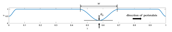
Figure 3: Visualizing the peristaltic activation wave

Here, speed of the peristaltic wave is denoted by $c$ and $L$ is the length of the FLIP bag. Substituting these into Eqs. (1), (4) and the parabolic version of Eq. (2) gives

$$\frac{\partial\alpha}{\partial\tau}+\frac{\partial\left(\alpha U\right)}{\partial\chi}=0,$$ (8)

$$\frac{\partial U}{\partial\tau}+U\frac{\partial U}{\partial\chi}+\psi\frac{\partial P}{\partial\chi}+\beta\frac{U}{\alpha}=0,\qquad\text{and}$$ (9)

$${\color[rgb]{0,0,0}P=\left(\frac{\alpha}{\theta}-1\right)-\eta\frac{\partial\left(\alpha U\right)}{\partial\chi}},$$ (10)

where the following non-dimensional numbers $\psi=K/(\rho c^{2})$, $\eta=(YcA_{0})/(KL)$ and $\beta=8\pi\mu L/(\rho A_{0}c)$ emerge. Here, $\eta$ is a nondimensional tube damping parameter and $\beta$ is a flow resistance coefficient. Eventually, the non-dimensional pressure $P$ in the momentum equation (9) will be replaced with the right hand side of Eq. (10). Thus, the total number of coupled equations to be solved is two with $\alpha$ and $U$ as the unknowns. When working with the friction factor version of the momentum equation, the non-dimensional number for flow resistance $\beta$ becomes $\left(fL/4\right)\sqrt{\pi/A_{0}}$ and $\psi$ remains unchanged and the viscous resistance term in the momentum equation takes the form $\beta U|U|/\sqrt{\alpha}$.

2.2 Boundary Conditions and Peristaltic Wave Input

It is clear that if $\eta$ is exactly zero, Eqs. (8), (9) and (10) allow only one boundary condition each for $\alpha$ and $U$ as the system is hyperbolic. However, during normal operation, the fluid volume inside the bag is constant because saline pumping is halted and the bag ends are sealed. Thus, fluid velocity at both ends must be set to zero which is not admissible with $\eta=0$. In addition to this, hyperbolic systems often present convergence issues. To address these issues, we set $\eta\neq 0$ and add a smoothing term $\epsilon\alpha_{\chi\chi}$ to the continuity equation [28]. Following this step, substituting Eq. (10) into Eq. (9) leads to second derivatives for $\alpha$ and $U$ requiring two BCs each for $\alpha$ and $U$ at both ends. The bag is attached to the catheter at both ends and tapers off to a point. Thus, boundary conditions for velocity at the ends,

$$U\left(\chi=0,\tau\right)=0\qquad\text{and}\qquad U\left(\chi=1,\tau\right)=0$$ (11)

are straightforward but the boundary conditions for nondimensional area $\alpha$ are unclear. Fixing the area to some nonzero constant value is equivalent to fixing the pressure and leads to an inconsistent problem definition. Boundary conditions for $\alpha$ must be consistent with BCs for $U$. We arrive at these by turning to Eq. (9) with $U=0$ at the ends which results in $\partial P/\partial\chi=0$. From Eq. (10), we see that this leads to

$$\frac{\partial\alpha}{\partial\chi}-\eta\left(U\frac{\partial^{2}\alpha}{\partial\chi^{2}}+2\frac{\partial\alpha}{\partial\chi}\frac{\partial U}{\partial\chi}+\alpha\frac{\partial^{2}U}{\partial\chi^{2}}\right)=0.$$ (12)

In the limit of $\eta\to 0$, this is equivalent to requiring $\partial\alpha/\partial\chi=0$ at both boundaries. Thus, we choose

$$\left.\frac{\partial\alpha}{\partial\chi}\right|_{\chi=0,\tau}=0\qquad\mathrm{and}\qquad\left.\frac{\partial\alpha}{\partial\chi}\right|_{\chi=1,\tau}=0$$ (13)

as Neumann-type boundary conditions for $\alpha$ at the tube ends. For nonzero damping, this BC is equivalent to changing the viscous resistance by an amount $-\eta\alpha U_{\chi\chi}$ at the ends. This additional resistance at the boundary will have negligible effect for small $\eta$. With the additional regularizing terms and applied BCs, the solution differs from the hyperbolic version at a thin region near the boundary. In the next section, using the Method of Manufactured Solutions, we show that the effect of damping on the overall solution is negligible. It should be noted that more complicated forms of the tube law can be used which account for longitudinal curvature, bending and tension [29, 30] in the tube wall. Such a tube law can include a double derivative, $A_{xx}$ or a fourth order derivative term $A_{xxxx}$ of the tube area. Under this setting, additional boundary conditions for area and pressure can be applied in a straightforward manner without leading to inconsistencies in the problem definition. The inclusion of these terms will lead to higher order spatial derivatives into the governing equations. However, in our current analysis, we choose to work with the simplest version of the tube law as the esophagus’ material properties and behavior for these deformation modes is unknown.

The last ingredient required to complete the model is specifying an activation input to mimic peristaltic contraction. We wish to induce a reduction in the tube area at some location $\chi$ and at some time $\tau$ in a manner that resembles a traveling peristaltic wave. The most common approach to induce contractions is seen in the aforementioned valveless pumping models where an external activation pressure at a specific location is varied sinusoidally with time [24, 23, 25]. This is an appropriate method of activation for valveless pumping scenarios due to the fact that the extra pressure is generated due to respiration. However, in the esophagus, contractions in area are generated due to a contraction of muscle fibers within the esophageal wall. As such, we add an activation term $\theta$ to the tube law which changes the reference area of the tube when activated. The tube law used is

$$P=\left(\frac{\alpha}{\theta}-1\right)-\eta\frac{\partial\left(\alpha U\right)}{\partial\chi},$$ (14)

with the activation term given by

$$\theta(\chi,\tau)=\begin{cases}1-\left(\frac{1-\theta_{0}}{2}\right)\Big{[}1\ +\\ \qquad\sin\left(\frac{2\pi}{w}\left(\chi-\tau\right)+\frac{3\pi}{2}\right)\Big{]},&\tau-w\leq\chi\leq\tau\\ 1,&\text{otherwise.}\end{cases}$$ (15)

The non-dimensional width of the peristaltic wave is denoted by $w=W/L$ with $W$ denoting the dimensional contraction width. As mentioned earlier, the CSA at the tube ends in the device tapers off to a point on the catheter, so a small correction is made to the activation term to account for the reduced CSA at the ends. The final form of the activation wave is plotted in Fig. 3. The value of $\theta_{0}$ specified represents the reference area of the tube at the strongest part of the contraction. Physiologically speaking, $\theta_{0}$ is a parameter that determines the strength of the contraction. It represents the ratio by which the zero-stress luminal area is reduced (i.e. the reference luminal area $A_{0}$) due to muscular contraction. The smaller the value of $\theta_{0}$, the smaller is the activated reference area and the greater is the contraction intensity. When $\theta_{0}=1$, there is no contraction and the system is fully at rest. Since the velocity scale was chosen to be the same as the speed of the peristaltic wave, the non-dimensional wave speed is 1.0.

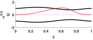
Figure 4: Tube shape (black lines) and fluid velocity (dotted red line) corresponding to the manufactured solution given by Eqs. (22) and (23) for $\tau=0.38$

2.3 Numerical Solution of the System of Equations

The non-dimensional pressure term $P$ in the momentum equation is eliminated using Eq. (14), which leads to the system of equations

$$\frac{\partial\alpha}{\partial\tau}+\frac{\partial(\alpha U)}{\partial\chi}=\epsilon\frac{\partial^{2}\alpha}{\partial\chi^{2}},$$ (16)

$$\frac{\partial U}{\partial\tau}+U\frac{\partial U}{\partial\chi}+\beta\frac{U}{\alpha}+\psi\frac{\partial}{\partial\chi}\left(\frac{\alpha}{\theta}\right)=\zeta\frac{\partial^{2}}{\partial\chi^{2}}\left(\alpha U\right),$$ (17)

with boundary conditions given by Eqs. (11) and (13). The product of $\eta$ and $\psi$ is denoted by $\zeta$. As explained earlier, a smoothing term $\epsilon\left(\alpha_{xx}\right)$ was added to the right hand side of Eq. (8) to accelerate convergence and reduce computation time. We set zero velocity initial conditions and specify a spatially-constant initial condition for area that depends on the volume of fluid present in the bag,

$$U\left(\chi,\tau=0\right)=0\qquad\qquad\alpha\left(\chi,\tau=0\right)=\alpha_{\text{IC}}.$$ (18)

This set of equations is solved using the pdepe routine in MATLAB. For the sake of clarity, we rewrite the final version of the governing equations and the boundary conditions in the form solved using MATLAB below (subscripts denote partial derivatives with respect to that variable):

$${\color[rgb]{0,0,0}\left[\begin{array}[]{c}\alpha_{\tau}\\ U_{\tau}\end{array}\right]=\left[\begin{array}[]{c}\epsilon\alpha_{\chi}\\ \zeta\left(\alpha U\right)_{\chi}\end{array}\right]_{\chi}-\left[\begin{array}[]{c}U\alpha_{\chi}+\alpha U_{\chi}\\ UU_{\chi}+\beta\frac{U}{\alpha}+\frac{\psi}{\theta^{2}}\left(\theta\alpha_{\chi}-\alpha\theta_{\chi}\right)\end{array}\right]}$$ (19)

$$\left[\begin{array}[]{c}0\\ U\end{array}\right]+\left[\begin{array}[]{c}1\\ 0\end{array}\right]\left[\begin{array}[]{c}\epsilon\alpha_{\chi}\\ \zeta\left(\alpha U\right)_{\chi}\end{array}\right]=\left[\begin{array}[]{c}0\\ 0\end{array}\right]\quad\text{for}\quad\chi=0,1$$ (20)

Before proceeding with our analysis of the FLIP device with this mathematical model, we ensured that the damping terms introduced in the continuity and momentum equation did not adversely affect the computed solution. The Method of Manufactured Solutions was used to test the solution approach to ensure that the system of equations was being solved correctly. A sinusoidally expanding and contracting tube shape was chosen that generated an oscillating velocity field within the tube. The solution chosen for $\alpha$ at time $\tau=0$ was

$$\alpha(\chi,\tau=0)=f(\chi)=\frac{256}{9}\left(2\chi^{5}-5\chi^{4}+4\chi^{3}-\chi^{2}\right)+1$$ (21)

and the shape of the tube at all other times was set to vary as a standing wave and has the form

$$\alpha(\chi,\tau)=\left[f(\chi)-1\right]\cos(\omega\tau)+1.$$ (22)

Using the original form of the continuity equation given by Eq. (8), the velocity field corresponding to the chosen tube shape was found to be

$$U=\frac{\omega\sin(\omega\tau)}{(f-1)\cos(\omega\tau)+1}\int(f-1)d\chi.$$ (23)

A snapshot of the manufactured tube shape and fluid velocity is shown in Fig. 4. The left segment of the tube has reached the maximum area of $\alpha=1.5$ at $\chi=0.25$. At this instant, the right segment of the tube is beginning to expand and the left segment is contracting causing fluid to flow into the expanding section of the tube. This corresponds to a positive fluid velocity as shown by the dotted red curve. Eventually the right segment of the tube reaches its maximum area and begins to contract and the cycle continues with fluid traveling from one segment of the tube to the other in a periodic manner.

Using the nondimensional form of the momentum equation (9), the source term corresponding to the chosen solutions was found with values of $\beta$ and $\psi$ set to $10^{3}$ and $\omega=10$. Using the regularized version of the governing equations given by Eqs. (19) and (20), along with $\zeta=0.01$ and $\epsilon=10^{-4}$, the system was then solved to obtain $\alpha$ and $U$. Relative tolerance for the solver was set to $10^{-7}$. A comparison of the manufactured solution to the computed solution is given in Figs. 5 and 6. The agreement between the chosen and numerically computed solutions was found to be satisfactory indicating that the equations were being solved correctly and that the effect of the regularizing terms on the overall solution was negligible.

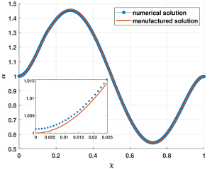
Figure 5: Comparison of the manufactured solution area and area obtained from the numerical solution of Eqs. (19) and (20) for $\tau=3.5$. Inset shows the variation of area at the boundary where the gradient was set to zero but the value was not kept fixed.

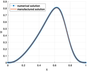
Figure 6: Comparison of fluid velocity obtained from the numerical solution of the regularized equations to the manufactured solution given by Eq. (23) at $\tau=3.5$

3 Dynamics Displayed by the 1-D Model

3.1 Comparison with 3D Immersed Boundary Simulations

Before proceeding with a discussion on the regimes and computing peristaltic work, we set out to further validate our 1D model with detailed fluid-structure interaction simulations using the immersed boundary (IB) method. It has already been stated that the nature of flow within the device is not definitively known to be either laminar or fully developed turbulent flow. As explained in Sec. 1.1, the Reynolds number for flow in the tube is estimated to be around 660, indicating that the flow is likely to be laminar. For healthy individuals, the value of $\psi$ is of the order 100 and $\beta$ is of the order 1000 based on known values of peristaltic wave speed [31], tube stiffness coefficient $K$ [26], and material properties of water. The material parameters for the 3D IB simulation were chosen such that they were equivalent to $\psi=100$, $\beta=621$ and $\theta_{0}=0.05$ and flow was observed to have a parabolic profile everywhere within the tube. Following peristaltic activation, the resulting tube shapes and fluid velocity variations obtained from both models were then compared.

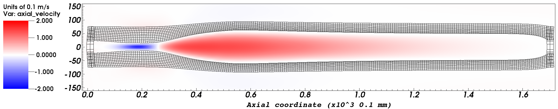
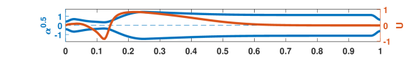
(a) Instant 1

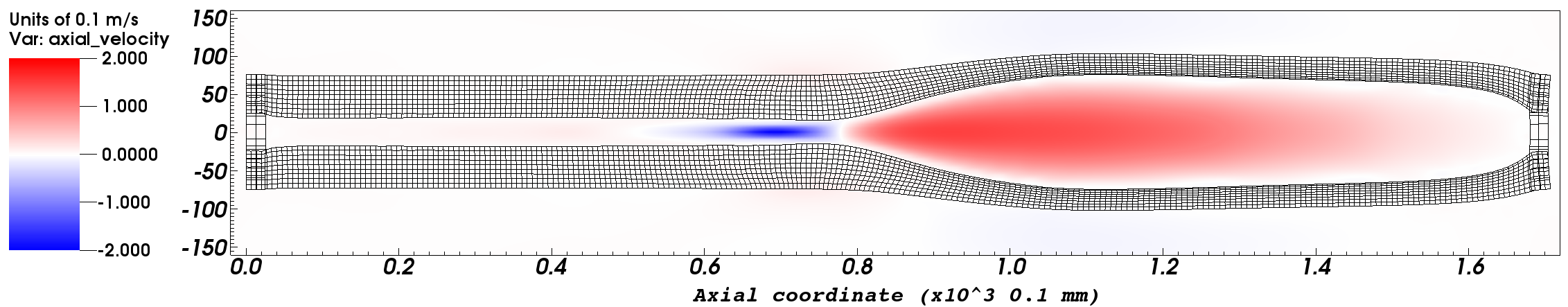
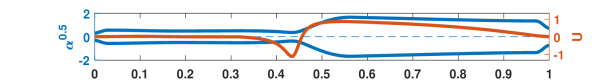
(b) Instant 2

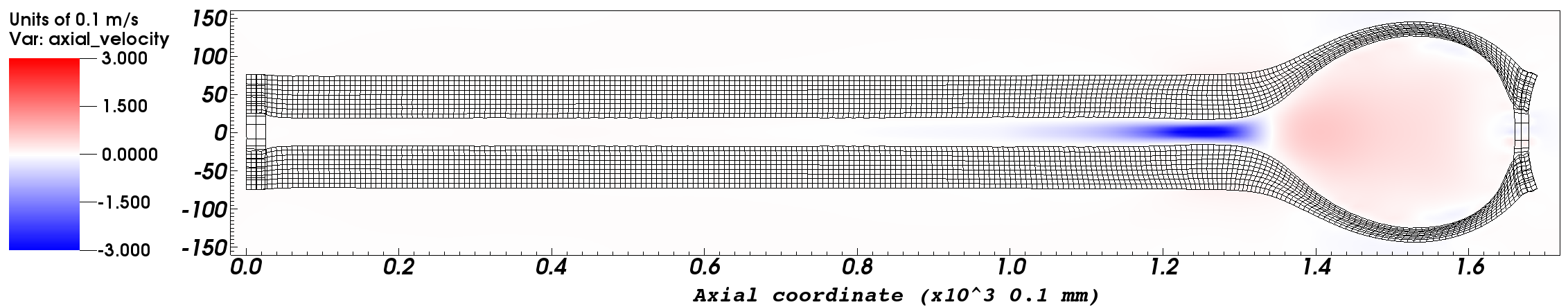
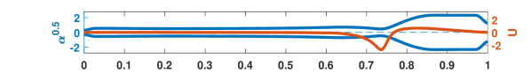
(c) Instant 3

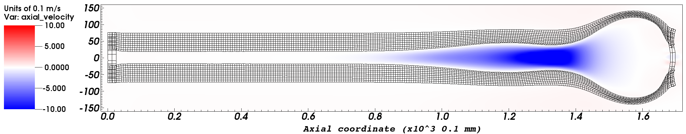
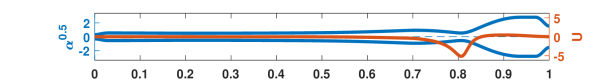
(d) Instant 4

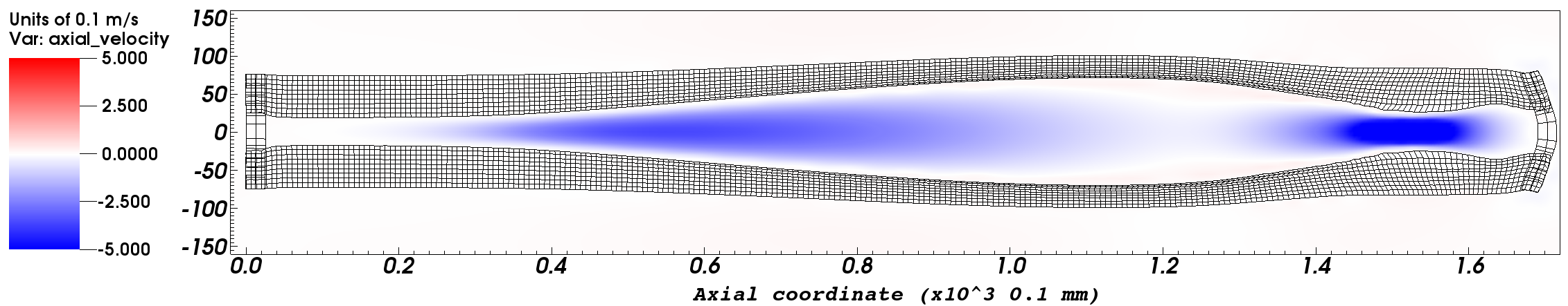
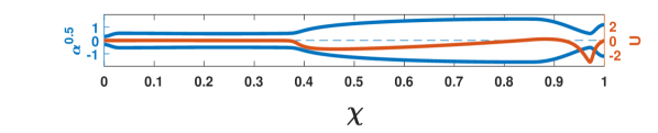
(e) Instant 5

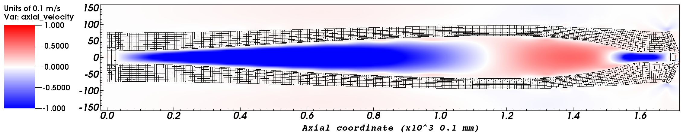
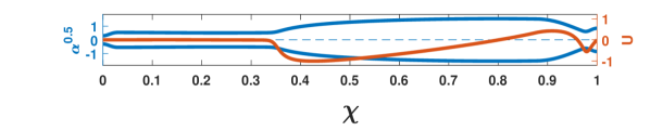
(f) Instant 6

Figure 7: Comparing tube shapes and velocity fields computed from the 1D model with results from equivalent 3D immersed boundary simulations. At each instant, the top figure shows the tube mesh along with the internal velocity fields along an axial slice obtained from the IB simulations and the bottom figure shows the corresponding variations predicted by the 1D model. In the latter, the blue curves plot the top and bottom profile of the tube using the nondimensional radius $\sqrt{\alpha}$ and the red curve shows the variation of velocity $U$ in the tube at each instant as a function of $\chi$. The dotted line represents the tube’s axis. Values corresponding to $\sqrt{\alpha}$ are on the left axis and values for $U$ are on the right axis. Negative values of $U$ indicate fluid is traveling in the left direction. Contraction wave began at $\tau=0$ and leaves the domain at $\tau=1$. Instants 5 and 6 correspond to $\tau=1.10$ and $\tau=1.13$, respectively. Figure 8 compares areas and the area-averaged axial velocity with $U$ from the 1D model for Instant 2.

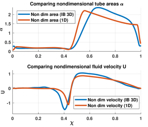
Figure 8: Quantitative comparison of nondimensional tube area and fluid velocity obtained from 3D IB simulations with the numerical solution of the 1D system of equations. This snapshot corresponds to Instant 2, shown in Fig. 7 where the contraction is approximately at $\chi=0.45$.

The geometry of the structure used in the IB simulations consists of a long cylindrical tube with open ends. The two ends are closed using ‘caps’ that are simply short flat cylinders of specified thickness. The entire structure is then meshed using hexahedral elements to take advantage of the Adaptive Anisotropic Quadrature that was developed by Kou et al., in [32] and implemented in the open-source immersed boundary framework IBAMR [33]. The structure is represented using finite elements and the combined fluid-structure equations are solved on a Cartesian grid using the Finite Volume Method. Mathematical details on the interaction equations, discretization of the Lagrangian and Eulerian domains and temporal schemes for solving the coupled system can be found in [34]. Computations were performed on the Northwestern University ‘Quest’ cluster and on SDSC Comet. The mechanical properties of the tube consists of two materials. Just like the esophagus, the structure in our IB simulations consists of fibers embedded in an isotropic matrix material. The matrix component is represented by a simple Neo-Hookean strain energy function and the fiber’s effect is implemented using a bilinear strain energy function that computes the stress based on strain in the circumferential direction. The combined effect of these layers leads to an approximately linear relationship between pressure and area corresponding to the tube law used in the 1D model. Additional details on the material properties and strain energy functions corresponding to each layer can be found in Refs. [32, 35, 20]. Similar to the activation method used in Ref. [32], the peristaltic wave is applied as a controlled reduction in the fiber rest length along the tube. This reduction leads to a greater generation of circumferential stresses in the tube at the activation location, the consequence of which is a reduction of the tube area resembling peristaltic contraction.

The results of our simulations are summarized in Figs. 7 and 8. The figures show the resultant tube shapes generated by the peristaltic contraction wave as it travels from left to right along the tube length for both models. As the contraction moves forward, it displaces fluid, causing an increase in tube area to accommodate the excess fluid. When the pressure in the segment ahead of the contraction becomes high enough, the contraction opens up, allowing fluid accumulated in this segment to flow in the opposite direction and refill the segment of the tube behind the contraction. Figures 7(e) and 7(f) show the tube profile and fluid velocity after the wave has passed. At each instant, we see satisfactory agreement between the velocity variations observed in the 3D immersed boundary simulations and the non-dimensional velocity profiles predicted by the 1D model. The tube shapes are also observed to match well with the shape of the structure computed by the 3D simulations during and after the activation wave has traveled over the tube’s length.

Encouraged by this agreement between the 1D model and the 3D immersed boundary simulations, we continued the analysis of the system by probing the 1D model for a wide range of operating conditions. Although the agreement was found only for parabolic flow, we also investigated the system’s response when the viscous term is friction-factor based. In the next section, we present the results for both of these scenarios in a “unified” regime map. One of the primary goals for this comparison with the 3D IB simulations was to check if the introduction of the tube damping and smoothing terms significantly affected the response of the system. Figures 7 and 8 show that that the introduction of the regularizing terms not only leaves the physics of the system unharmed but also aids in stabilizing the numerical solution which directly leads to more rapid solution times.

It should be noted that the 3D immersed boundary simulations did not show any modes of asymmetric collapse or solid-solid contact between the tube walls for the operating parameters that were tested. The cross section of the tube remained circular across its entire length for the entire duration of the run. The speed at which a disturbance propagates in the system is given by $\partial p/\partial A\sqrt{A/\rho}$ [29] and is approximately 1 m/s for the esophagus. The peristaltic wave speed and internal fluid velocities are of the order of 1 cm/s indicating that the flow speeds are always well below the critical value needed for collapse or choking. At the location of the contraction, the tube is not passive and the there is no collapse of the structure. The reduction in area is solely due to active contraction brought upon by a controlled reduction of the rest length of the fibers in the tube’s material model. It should also be emphasized that the coupled fluid-structure simulations we have developed are perfectly capable of capturing any event of collapse if there was a possibility for such an event to occur. However, for the range of parameters that are relevant to the operating conditions of this device, collapse is improbable due to the tube’s geometry and the significant amount of fluid in the bag (30 mL or greater). Another thing to note is that as the FLIP only measures area, comparison of simulation results with realistic three-dimensional structures is not possible at the moment. In the future, we aim to obtain detailed geometric information about the esophageal structure from fluoroscopy and 4D-MRI imaging [36] to compare numerical results with experimentally measured values.

3.2 Types of tube deformations observed during peristalsis

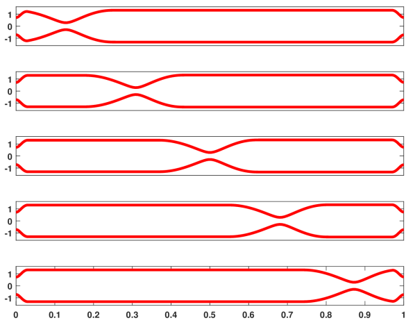
(a) Regime 1

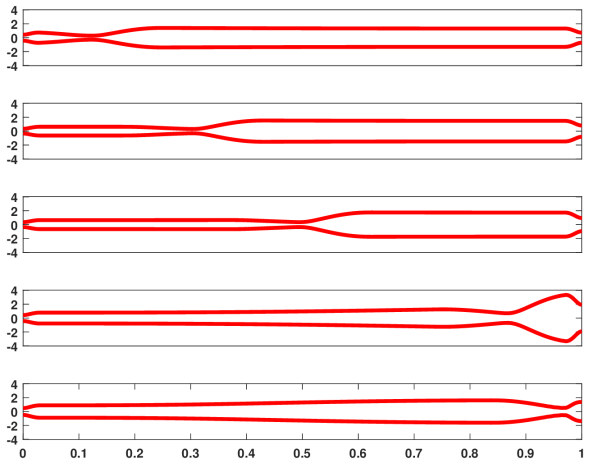
(b) Regime 2

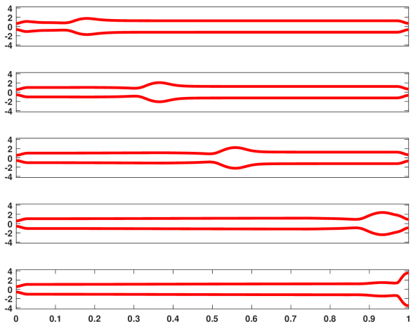
(c) Regime 3

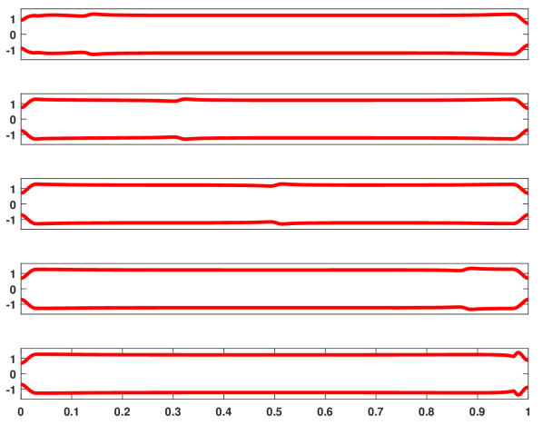
(d) Regime 4

Figure 9: Tube deformations corresponding to regimes occurring for physiologically relevant parameter ranges. Definitions used to classify a solution as belonging to a particular regime are given in Table 1.

With all the parts of the 1-D model in place, we can now investigate the system’s response to the applied activation as a function of the operating parameters, $\theta_{0}$, $\psi$ and $\beta$. Changing these values is equivalent to investigating the effect of tube wall stiffness, wave speed, contraction strength, fluid density and flow resistance on the tube wall deformation and internal flow patterns during peristalsis. After studying the system’s behavior for a broad range of operating values, we found four distinct, physiologically relevant patterns of peristaltic pumping based on the way the tube walls and the fluid inside respond to the applied activation. These regimes are shown in Fig. 9. The progression of these regimes from numbers 1 to 4 can be interpreted simply as the response of the system as fluid viscosity is continually increasing. It should be noted that the fourth regime displays very little deformation of tube area. The deformation dynamics for this regime are unremarkable and the tube shape remains quite similar to the shape of the initial condition for the entire duration.

The occurrence of these regimes is dictated by a competition between elastic forces generated due to deformation of the tube wall and resistance to flow through the narrowest part of the contraction. A relatively stiff tube wall resists deformation and forces the fluid that was displaced due to the advancing wave to flow back through the contraction. In this scenario, we see the walls deform as shown in Regime 1. An equivalent way of looking at this is to assume a low resistance to flow through the contraction. The energy required to expand the tube walls is significantly greater than the energy required to overcome viscous resistance across the contraction and thus, the pumping is almost quasi-steady with the tube walls having the same diameter on either side of the contraction. On the other hand, if the resistance to flow is high, it is favorable for the system to expand the tube walls to accommodate the fluid that is being displaced by the advancing peristaltic wave. At moderate flow resistances, this exact situation occurs when the stiffness of the tube walls is low. The tube deformation pattern in this scenario is denoted as Regime 2.

Regime 3 has been investigated in great detail by Takagi and Balmforth [11]. In their work, the lubrication approximation is used in an infinitely long domain with open ends. In our configuration, we see the formation of a “blister” as predicted by their model when the resistance to flow is high and the tube walls are fairly compliant. The formation of a blister is due to the fact that the amount of time it takes for the fluid to redistribute is comparable to the time it takes for the wave to travel along the tube length. Regime 4 occurs when the resistance to flow is much higher than that in Regime 3. In this case, the amount of time it takes for the fluid to ‘move’ and respond to the peristaltic contraction is much higher than the amount of time it takes for the wave to travel over a section of the tube. The fluid velocity in this case is extremely low leading to a small value in $\partial A/\partial t$ as well. In this region of operation, the fluid essentially behaves as a semi-solid entity and the contraction causes only a small local deformation as it travels forward.

When the value of $\psi$ (which is the inverse of the Mach number squared) is small, the wave-like nature of the system begins to emerge. In this region the speed of the peristaltic wave is comparable to the speed at which a disturbance in the system travels at. For the esophageal wall, this disturbance speed is of the order of 1 m/s, but the peristaltic wave speed rarely exceeds 10 cm/s. As such, we will not investigate the dynamics of the system at these unphysiologic wave speeds.

4 System behavior represented as a regime map

In Section 3, four patterns of observed tube wall deformation depending on the system’s operating conditions were presented (Fig. 9). Our goal was to combine the various operating parameters to summarize the response of the system in the form of a regime map. We wished to find the least number of parameters that could be used to describe the response of the system to the peristaltic contraction wave. Using the Buckingham-Pi approach leads to the several non-dimensional numbers already shown above. Plotting the system’s response for each of these quantities is cumbersome. To that effect, we utilized the wave-frame approach that has often been employed by other researchers to analyze peristaltic flow to find the most convenient combination of operating parameters to visualize the system’s response. Detailed derivation of these parameters is provided in the Supplemental Materials section on the ASME Digital Collection.

From the wave frame-based analysis based on Fig. 11, we systematically combined the tube stiffness coefficient, contraction properties, fluid viscosity and peristaltic wave speed to obtain two nondimensional numbers: cumulative flow resistance $\psi_{f}^{\prime}$ (or $\Psi_{f}^{\prime}$) and cumulative stiffness $\psi_{k}^{\prime}$ that were used to describe the system’s response to a peristaltic contraction. Depending on the specific version of the viscous term used (parabolic flow or friction factor-based) in Eq. (2), $\psi_{f}^{\prime}$ or $\Psi_{f}^{\prime}$ is computed from the input parameters. The two terms $\psi_{k}^{\prime}$ and $(\psi_{f}^{\prime},\ \Psi_{f}^{\prime})$ together, account for all the relevant parameters of the system. The effect of tube stiffness, fluid density, wave velocity and the amount of fill volume of the tube is accounted for in $\psi_{k}^{\prime}$ and $\psi_{f}^{\prime}$ accounts for the fluid’s resistance to flow in the tube, the length of the contraction zone and its intensity. All of these effects contribute to the increase or decrease of the area ratio $A_{2}/A_{1}$ and hence the observed regime. The utility of our analysis is now clear because if we wished to visualize the effect of these variables on pumping patterns, we would either need several figures or utilize a plot that has multiple axes, corresponding to wave velocity, tube stiffness, fluid viscosity, etc. However, by combining these parameters in a sensible manner, made possible by the wave-frame analysis, the visualization of observed regimes can be achieved in a clear and coherent way. The final combination of operating parameters used to compute these cumulative nondimensional numbers is

$$\psi_{k}^{\prime}=2\psi\alpha_{\mathrm{IC}}=2\left(\frac{K}{\rho c^{2}}\right)\alpha_{\mathrm{IC}}$$ (24)

$$\psi_{f}^{\prime}=2\beta w\left(\frac{1-\theta}{\theta^{2}}\right)\quad\mathrm{for\ Low\ Re\ with\ \ }\beta=\frac{8\pi\mu L}{\rho A_{0}c}$$ (25)

$$\Psi_{f}^{\prime}=2\beta w\left(\frac{1}{\sqrt{\theta}}\right)\left(\frac{1-\theta}{\theta}\right)^{2}\quad\mathrm{for\ High\ Re\ with\ \ }\beta=\frac{fL}{2D_{0}}$$ (26)

Figure 10: Regime map showing system’s response for a variety of input conditions for both parabolic and friction factor-based flow resistance terms. The parameters $\psi_{f}^{\prime}$ and $\psi_{k}^{\prime}$ are computed using Eqs. (24), (25) and (26) for each data point. The x-axis represents a cumulative stiffness parameter and the y-axis represents a cumulative flow resistance parameter. Legend: Regime 1 ($\color[rgb]{1,0,0}\blacktriangle$), Regime 2 ($\color[rgb]{1,0,1}\boldsymbol{\times}$), Regimes 3,4 (_∙)

The system’s response was investigated for a wide range of physiologically relevant parameters. Values of $\psi$ were selected from the following set: {0.1, 0.25, 0.6, 1, 2.4, 5, 10, 24, 50, 100}$\times 10^{3}$ and $\beta$ had the following values: {0.1, 0.25, 1, 5, 10, 50, 100, 250}$\times 10^{3}$. Two values of the initial condition $\alpha_{IC}$={1.25, 2.0}, corresponding to the volume of fluid in the tube, were chosen. The following values for contraction intensity $\theta_{0}$ were selected: {0.05, 0.1, 0.15, 0.2}. The nondimensional width $w$ was set to 0.25 for all runs. All possible combinations of these parameters leads to 640 cases each for the parabolic and friction factor-version of the momentum equation. The damping parameters and solver tolerance were set to the same values that were used during verification using the Method of Manufactured Solutions. Volume of fluid in the tube was monitored as a measure of solution accuracy. Percent change in tube volume across all runs was of the order of $10^{-11}$. The tube shape computed from each of these runs was analyzed when the contraction was at the halfway point i.e. at $\chi=0.5$. At this instant, the ratio $A_{2}/A_{1}$ was computed along with the maximum tube area achieved ($A_{\mathrm{max}}$) and area of the contraction ($A_{c}$). Based on visual inspection of their values for several cases, the tube shape was then classified as Regime 1, 2 or 3/4 using the definitions provided in Table 1. Complete parametric information and the associated regime for each case plotted in the regime map is provided in a data sheet available in the Supplemental Materials on the ASME Digital Collection.

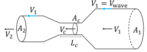
Figure 11: Peristaltic contraction as observed in the wave’s frame of reference

Table 1: Definitions used to classify each solution as belonging to a particular regime

Regime 1		${A_{1}}/{A_{2}}<1.7$
Regime 2		${A_{1}}/{A_{2}}\geq 1.7$
Regime 3		$A_{\mathrm{max}}/{A_{1}}>1.5$
Regime 4		$A_{c}/A_{2}>0.9$

Note: Areas $A_{1}$ and $A_{2}$ are the distal and proximal areas (Fig. 11) and $A_{\mathrm{max}}$ is the area of the bulge (observed in Regime 3 only) at its widest point. For Regimes 1 and 2, $A_{\mathrm{max}}=A_{1}$. The area at the contraction is denoted by $A_{c}$.

Armed with this simplification, we present the occurrence of each regime as a set of points on a $\psi_{f}^{\prime}$ vs. $\psi_{k}^{\prime}$ plot. Fig. 10 shows the occurrence of the various regimes at different values of the two $\psi^{\prime}$s. We combine all the regime points from the two different flow types and present them in a single plot. We see that the regime data points from both flow types fall within the general vicinity of each other. The set of points belonging to each regime is represented by a specific marker.

The wave frame approach that was taken to find the combination of parameters does not account for the formation of a bulge or a blister. As both regimes 3 and 4 occur in the region of high fluid viscosity, they are combined into a single entity for plotting purposes. From this plot, we clearly observe the presence of a general boundary between each set of regime points. The boundary represents the change of the system from one solution to another. This analysis can be used as a starting point to quantitatively derive the location of the boundaries between the regimes shown in Fig. 10. In addition to the parameters mentioned above, it has been observed that there is active relaxation ahead of, and stiffening behind, the contraction wave that can change the effective material properties of the tube to improve bolus transport through the esophagus [37, 38]. In a future work, we will be incorporating these non-uniform changes in effective material properties into our analysis and study the effect on the observed regimes and quantitatively predict the regime boundaries as a function of all physiologically relevant parameters.

With the help of the regime map, one can predict the shape assumed by the tube during peristalsis by simply computing the relevant $\psi_{f}^{\prime}$ and $\psi_{k}^{\prime}$ from the given operating conditions and finding the region which these points belong to. The regime map also helps in understanding the change in tube shape that would occur as one of the operating conditions is changed. For instance, as the tube stiffness increases, the system will deform in such a way that the area ratio tends to 1.0. Increasing the fill volume or decreasing the peristaltic wave velocity leads to a similar outcome. When it comes to increasing the fluid’s viscosity, we see a transition from Regime 1 to Regime 2 as predicted by the regime map when the value of $\psi_{f}^{\prime}$ is increased. When the area contraction factor $\theta$ is reduced i.e. the amount of wave ‘squeezing’ is increased, we again observe the system transition from Regime 1 to Regime 2.

Each of these regimes correspond to a specific deformation pattern observed using the FLIP device in different subjects and/or diseases. For instance, assume that the device is calibrated and the operating conditions are benchmarked in such a way that it shows pumping patterns corresponding to Regime 2 in a healthy individual. Under the same operating conditions, a patient with peristaltic dysfunction will display pumping patterns corresponding to either Regime 1 or Regime 3/4. Depending on the specific behavior displayed, the regime map helps us identify the cause of the abnormality. For instance, a patient displaying regime 1 might have a stiffer esophagus due to fibrosis and a patient with Regime 4 has dysphagia due to ineffective peristalsis. Thus the quantification of the device’s behavior in the form of these regime maps directly assists in better interpreting the various shapes seen in patients during the FLIP procedure.

5 Defining and quantifying pumping effort

In this section, we aimed to understand how energy is spent during a peristaltic contraction in a closed tube. Finding the work done by a peristaltic wave and observing its variation during pumping can offer further insights into the pumping process. The configuration that is being analyzed in this work is a closed system. As such, there is no “net flow rate” or non-zero displacement of fluid volume during one peristaltic event which can be used to quantify efficacy. At the end of peristalsis, all the work done by the peristaltic wave is dissipated due to fluid viscosity. Hence, the total pumping work done is simply the amount of energy that has dissipated. During peristalsis however, the stretching of the esophageal walls leads to some of the energy being stored as elastic potential energy. After passage of the peristaltic wave, the tube relaxes and releases the energy back into the fluid which is then lost via viscous dissipation. To understand the quantitative relationship between these three agents, we turn to the parabolic version of the momentum equation (2) and multiply both sides with $Au$ to obtain

$$\rho Au\frac{\partial u}{\partial t}+\rho\left(Au\right)u\frac{\partial u}{\partial x}=-Au\frac{\partial p}{\partial x}-\frac{8\pi\mu Qu}{A}.$$ (27)

Noting that $Q=Au$, we rewrite the equation to form terms that involve derivatives of the kinetic energy of the fluid per unit volume. We end up with

$$A\frac{\partial}{\partial t}\left(\frac{1}{2}\rho u^{2}\right)+Q\frac{\partial}{\partial x}\left(\frac{1}{2}\rho u^{2}\right)=-Au\frac{\partial p}{\partial x}-\frac{8\pi\mu uQ}{A},$$ (28)

to which we add the continuity equation (multiplied with $\rho u^{2}/2$) on the LHS and after combining terms using the product rule, we end up with the equation

$$\frac{\partial}{\partial t}\left(\frac{1}{2}\rho Au^{2}\right)+\frac{\partial}{\partial x}\left(\frac{1}{2}\rho Qu^{2}\right)=-Au\frac{\partial p}{\partial x}-\frac{8\pi\mu uQ}{A},$$ (29)

the terms of which can be interpreted as follows,

$$\frac{\partial}{\partial t}\left(\frac{1}{2}\rho Au^{2}\right)+\frac{\partial}{\partial x}\left(\frac{1}{2}\rho Qu^{2}\right)=-\underbrace{\frac{\partial\left(Aup\right)}{\partial x}}_{\text{surface work}}+\underbrace{p\frac{\partial\left(Au\right)}{\partial x}}_{\sim\ p\nabla\cdot\mathbf{u}}-\underbrace{\frac{8\pi\mu uQ}{A}.}_{\begin{subarray}{c}\text{viscous}\\ \text{dissipation}\end{subarray}}$$ (30)

Note that conservation of volume can be used to replace the $\partial\left(Au\right)/\partial x$ term with $-\partial A/\partial t$ to obtain

$$\frac{\partial}{\partial t}\left(\frac{1}{2}\rho Au^{2}\right)+\frac{\partial}{\partial x}\left(\frac{1}{2}\rho Qu^{2}\right)=-\frac{\partial\left(Aup\right)}{\partial x}-p\frac{\partial A}{\partial t}-\frac{8\pi\mu uQ}{A}.$$ (31)

Now we integrate this equation over the length of the tube from $x=0$ to $L$ and apply the zero velocity condition $Q=u=0$, at the tube ends. This leads to terms with $\partial x$ going to zero giving

$$-\int\limits_{0}^{L}p\frac{\partial A}{\partial t}\mathrm{d}x=\frac{\partial}{\partial t}\int\limits_{0}^{L}\left(\frac{1}{2}\rho Au^{2}\right)\mathrm{d}x+\int\limits_{0}^{L}8\pi\mu u^{2}\mathrm{d}x.$$ (32)

Equation (32) succinctly shows how power is distributed in the system at each time instant. Without the negative sign, the pressure term represents the work done by the fluid on the tube walls. Thus, the LHS is the work done by the walls on the fluid. The first term on the RHS is the rate of change in the kinetic energy of the fluid and the last term is the rate of energy loss due to viscous dissipation. It is important to realize that the pressure term has contributions from both the passive elastic part of the esophageal walls and the rise due to active contraction. When separated, we get a better understanding of the power breakdown,

$$-\int\limits_{0}^{L}p_{\text{actv}}\frac{\partial A}{\partial t}\mathrm{d}x=\frac{\partial}{\partial t}\int\limits_{0}^{L}\left(\frac{1}{2}\rho Au^{2}\right)\mathrm{d}x\ +\int\limits_{0}^{L}p_{\text{pass}}\frac{\partial A}{\partial t}\mathrm{d}x+\int\limits_{0}^{L}8\pi\mu u^{2}\mathrm{d}x.$$ (33)

Simply put, the LHS is the rate of work done by the active part of the tube wall (the peristaltic contraction) on the confined fluid and the terms on the RHS show the consumers of this spent power. Some of it goes into increasing the kinetic energy of the fluid, some of it is stored in the tube walls when they stretch due to an increase in local pressure and the rest is lost due to viscous dissipation. At this point, we need to assume some form of the passive pressure to compute the values of each these terms for the various regimes displayed in our 1D model. The most logical form of the passive pressure component is a linear dependence on the tube area as seen in [26]. The breakdown of the fluid pressure can then be trivially split as

$$P=\frac{\alpha}{\theta}-1=\underbrace{\left(\alpha-1\right)}_{\text{passive}}+\underbrace{\alpha\left(\frac{1}{\theta}-1\right)}_{\text{active}}.$$ (34)

Using this breakdown of fluid pressure, we can compute the values of each of the terms in Eq. (33) and visualize the variation of work done or energy dissipated over a single peristaltic event for each regime. The above analysis can be repeated for the momentum equation with the friction factor stress term but the resulting work variations show no qualitative differences between the two scenarios.

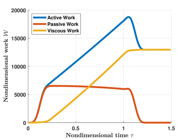
(a) Regime 1

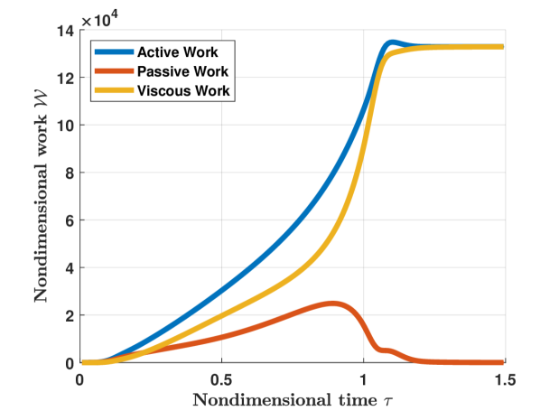
(b) Regime 2

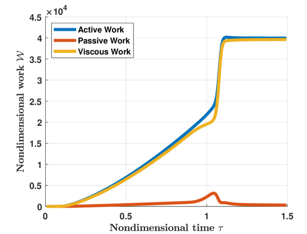
(c) Regime 3

Figure 12: Representative work curves for regimes that show non-trivial tube deformation. Each regime shows a unique signature for variation of work during peristalsis. At each instant, the sum of passive and viscous work is equal to the active work done.

5.1 Work curves from the reduced order model

As explained earlier, Eq. (33) gives the balance of power at each instant of time. Integrating this equation over time gives the balance of work done or energy lost as the peristaltic wave advances. In Fig. (12), we show the energy contribution from each of these terms for regimes with non-trivial tube shapes. This figure summarizes how the active work is split between the two sinks over the entire range of observed pumping patterns. At time $\tau=0$, the peristaltic wave begins traveling over the tube length and the active work done by it is zero. As the wave advances, the work done by it i.e. the active work is split into either increasing the potential energy stored in the tube walls or generating flow fields that then lose energy via dissipation. For the parameter space that is being analyzed in this work ($\psi\gg 1$), the rate of change of fluid kinetic energy is negligible and has not been plotted. Non-dimensionalizing Eq. (33) results in

$$-\psi\int\limits_{0}^{1}P_{\text{actv}}\frac{\partial\alpha}{\partial\tau}\mathrm{d}\chi=\frac{\partial}{\partial\tau}\int\limits_{0}^{1}\left(\frac{1}{2}\alpha U^{2}\right)\mathrm{d}\chi+\psi\int\limits_{0}^{1}P_{\text{pass}}\frac{\partial\alpha}{\partial\tau}\mathrm{d}\chi+\beta\int\limits_{0}^{1}U^{2}\mathrm{d}\chi,$$ (35)

which shows that for large values of $\beta$ and $\psi$ (as is the case for flows relevant to esophageal peristalsis), the term corresponding to rate of change of fluid kinetic energy is very small compared to the other terms in the energy balance equation.

The work curves for each of these regimes show unique identifying features that confirm what is visually observed through the tube deformation patterns. For Regime 1, once the wave has created a zone of reduced area, the active work goes into overcoming the viscous resistance and the potential energy stored in the walls remains unchanged. Upon approaching the right boundary, the contraction leaves the domain causing the tube to relax and the stored elastic energy is recovered. For Regime 2 however, we observe a gradual rise in stored elastic energy with time indicating that the activation wave is continuously doing work on the tube wall. Unlike Regime 1, when the wave approaches the end and allows the tube walls to relax, the stored energy is lost via fluid dissipation. This is observed by following the viscous work curve which sharply rises around the $\tau=0.8$ mark to meet the active work curve. It is also interesting to note that in spite of large tube wall deformations associated with this regime, the majority of active work done is still lost via viscous dissipation. Work curves for Regime 3 reflect the low wall deformations observed from the tube shape plots which only show a bulge ahead of the contraction. The passive work done is small compared to the active work done which is almost entirely lost via viscous dissipation. When the contraction approaches the end, it acts on the bulge in the tube ahead of it as it cannot go any further. Contraction of this bulge then reduces its area and causes the accumulated fluid to flow in the opposite direction. This leads to the sharp rise in viscous work at $\tau=1$ as seen in Fig. 12(c). For Regime 4 there is a simple, linear increase in viscous dissipation with time. Passive work done is zero for all time due to negligible wall deformation.

This detailed look into the variation of the active, passive and viscous work done during a peristaltic event gives us the tools to identify what a healthy pumping wave looks like and the conditions under which one might observe reasonable tube wall deformations. A significant change in the tube area for this configuration due to peristalsis (as seen with the healthy peristaltic wave in Fig. 2) indicates that the wave has some ability to move fluid forward in a normal setting which involves bolus transport following normal swallowing.

5.2 Work curves from FLIP patient data

In the previous subsection, we have defined and provided a strong mathematical foundation for computing work done during peristalsis in the current configuration and the various sinks that consume the energy generated by muscular activation. The work calculations were performed in the context of the reduced order model presented in Section 2. In this section, we wish to extend the utility of the model to compute work curves using data obtained from the FLIP device when used in human subjects. The goal was to get a sense of the magnitude of peristaltic work done in normal subjects and to see what characteristics are observed in work curves obtained from patient data.

It is clear that the 1D model in Section 2 takes as input the activation wave and predicts the resultant tube wall deformation and the associated fluid velocity and pressure fields. The FLIP data on the other hand contains the variation of tube wall deformation as a function of time and the value of pressure at the (approximate) location $x=\chi L=16\ \mathrm{cm}$. Simply speaking, $A(x,t)$ and $p(L,t)$ are already known. The values of fluid velocity and pressure at all the other locations along the tube are unknown. The device measures the lumen profile and stores diameter readings from each of the 16 sensors (as seen in Fig. 1). The recorded diameters are used to compute lumen area after accounting for the catheter’s presence and are corrected to ensure volume conservation in the tube. Equation (1) is then used to calculate $U(x,t)$ from planimetry data $A(x,t)$ collected by the device. With the available values of $A(x,t)$ and $U(x,t)$, the momentum equation (2) is used to compute the pressure gradient. Using $p(L,t)$, the pressure is then found as a function of $x$ and $t$ for the entire duration of peristalsis. Implementation details of this step using Eqs. (8) and (9) are provided in Ref. [39].

With these steps in place, we isolate a contraction wave to analyze and generate work curves for. An example of this can be seen in Fig. (2). A window of readings is chosen that includes a single pressure peak. At the start of computation, the wave begins to travel over the tube length and results in a pressure rise. The contraction travels along the esophagus as time goes on and by the last reading the wave has finished traveling over the entire tube length and the computation ends. In Fig. (13), we show the work curves and the pressures at $\chi=0.2$ (referred to as the proximal pressure) and $\chi=1$ (referred to as the distal pressure) as a function of time for a typical peristaltic contraction. Again, we emphasize that the former is predicted by our model and the latter is measured by the device and is applied to the model to fix the pressure levels inside the tube.

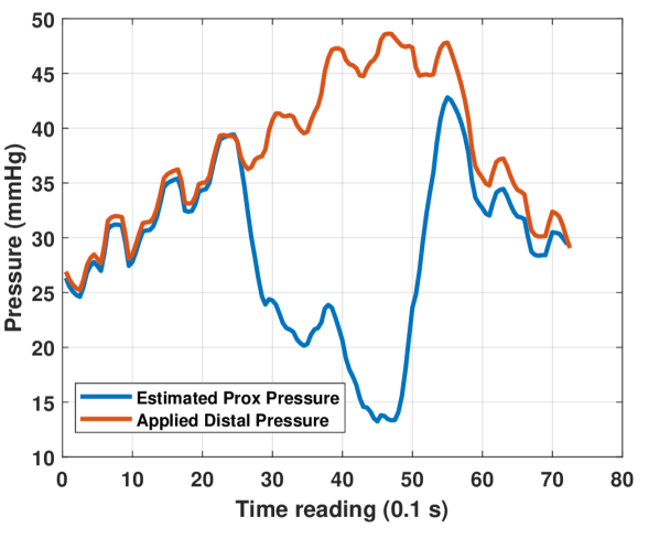
(a) Contraction 1 - pressure variations

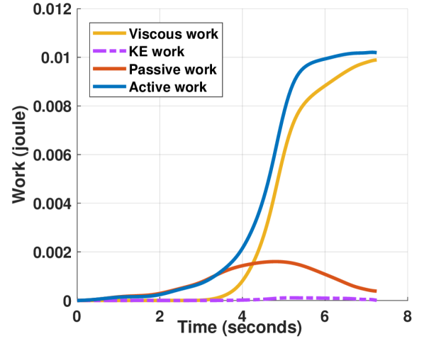
(b) Contraction 1 - work vs. time curves

Figure 13: Estimated proximal pressure variation and work computations from FLIP data corresponding to a single peristaltic contraction occurring at 30 mL in a healthy control. The esophagus does not return to its exact starting shape at the conclusion of peristalsis leading to a small non-zero value of passive work at the end.

The first thing to note from the analysis of the patient’s secondary peristaltic contractions is the pressure predicted by the model at the proximal (left) end of the tube at $\chi=0.2$. When the wave is incoming, the pressure in the entire system rises, but once it passes over the left end, there is a sharp drop in pressure. This is due to the temporary displacement of fluid due to the peristaltic pumping action of the wave leading to the tube having reduced area at the left end. The displaced fluid then stretches the walls of the distal end of the tube at $\chi=1$ and this is marked by the continuous rise in pressure at that location. Once the wave has passed, the fluid accumulated at the end flows back and the tube attains a uniform shape and pressures at both locations equalize at the end of wave travel. This development of a proximal pressure trough has also been observed in a FLIP prototype where there was an additional pressure sensor near the proximal end. Due to inaccuracy in the sensor, the readings have not been plotted. Qualitatively speaking, however, the readings showed a drop in pressure which is supported by our calculations.

The work curves shown in the right column of Fig. 13 are computed from the estimated fluid pressure and velocity fields. The curves show the same behavior observed in the curves derived from the 1D model i.e. the work done to change the kinetic energy of the fluid is minimal and the active work done is mostly lost via viscous dissipation. The calculation of active and passive work done from the 1D model in Section 5.1 depends on the value of $\theta$ which is completely known. However, the activation strength is not available from real-world patient data, as such estimating the breakdown of the pressure work term into an active and passive component is difficult. To get around this hurdle, we use the FLIP data to get the tube’s reference area $(A_{0})$ and the tube stiffness constant ($K$) when the esophagus is fully relaxed. Once this information is obtained, the passive power was estimated as

$$\mathcal{P}_{pass}=\int_{0}^{L}p_{\text{pass}}\frac{\partial A}{\partial t}\mathrm{d}x=\int_{0}^{L}K\left(\frac{A}{A_{0}}-1\right)\frac{\partial A}{\partial t}\mathrm{d}x.$$ (36)

The active work is then estimated by subtracting the passive work from the total fluid pressure work. These estimated values of passive and active work are then plotted in the work curves shown in Fig. 13(b). The passive work is again seen to be smaller than the magnitudes of active and viscous work. One observation from these curves is that the total magnitude of work done for a single healthy secondary peristaltic contraction is of the order of $10$ millijoules (mJ). Studies conducted using traction force sensors have been able to quantify the propulsive force generated by the esophagus during peristalsis [31]. On the lower end of the spectrum, the esophagus was able to generate 0.11 N of force. During FLIP examinations, around 12 cm of the bag lies within the segment of the esophagus that undergoes peristaltic contraction. Using these values of force and distance, a rough estimate of the work done was found to be 13.2 mJ which is of the same order of magnitude as predicted by our model. In a separate clinical study, we compute the work done for several controls and patients belonging to four disease groups to understand differences in peristaltic work done. [40]

6 Model Limitations

In this section, we discuss a few limitations of the 1D model developed to study the FLIP device and its response to peristaltic contraction.

During particularly strong peristaltic activity, circular muscle contraction can obliterate the esophageal lumen and completely cut off the proximal and distal segments of the tube from each other. In this scenario, both velocity $U$ and area $\alpha$ in the contraction region are zero and the model becomes singular. However, in a majority of peristaltic contractions studied with the FLIP, flow is observed to occur between chambers indicating nonzero $\alpha$ and $U$ in this region.

Another avenue of exploration is the effect of nonlinear tube laws on the quantity of work done during peristalsis. The complex fiber architecture of the esophageal wall is one reason for this nonlinear behavior. The other reason is the polyurethane bag used in the device. For bag volumes beyond 40 mL, there is greater stretching of the bag walls. When fully stretched, they sharply resist further dilation. This sudden increase in stiffness might have a significant effect on the estimate of work done. The esophagus’ material properties vary along its length as well. The exact variation of these properties is unknown, so as a first step, we assumed a simple linear tube law to estimate work. Additionally, tube laws that incorporate viscoelasticity will also significantly increase the amount of work done as the energy lost within the walls due to hysteresis will be considered.

Finally, the peristaltic activation wave does not have a constant velocity. The wave can speed up or even completely stop depending on the amount of obstruction it senses as a form of feedback regulation. In our configuration, this can become quite important as the ends are closed and continuous pumping will lead to a larger obstruction which can alter the speed and intensity of contraction in subjects, directly affecting the work done by the wave. Another detail that has not been considered is the precise positioning of the bag within the esophagus. When deployed by the physician, part of the bag straddles the Esophagogastric junction (EGJ) and the tip lies within the stomach. The EGJ is a physiologically complex region that behaves quite differently compared to the rest of the esophagus. In our work, we have assumed that the entire bag rests within the esophagus.

7 Concluding remarks

In this work, we have analyzed a hitherto unstudied configuration of fluid flow in an elastic tube. A simple reduced-order model is presented that is able to predict fluid flow and the resultant tube wall deformation when a peristaltic wave passes over a closed cylindrical tube. The model has been compared to detailed three-dimensional immersed boundary simulations and is shown to have satisfactory agreement with them. The system’s response under this set of operating conditions has been thoroughly quantified and visualized as a regime map.

Finally, the system’s utility is demonstrated by applying it to enhance the data collected with balloon dilation catheters. Paired with this tool, the device can now be thought of as having multiple pressure and velocity sensors housed on the catheter. With the help of these quantities, an appropriate mathematical foundation was laid to quantify the peristaltic work done. This step has led us to estimate the work done by the esophagus during a healthy contraction under these operating conditions. The device can now be used to find work done in other peristaltic waves and comment on their capability to propel fluid.

The analysis has a few limitations due to the inherent complexity of the combined organ-device system. However, the model presented in this work provides a foundation on which future studies can be based and used to further our understanding of esophageal pumping processes.

Funding Data

• National Institutes of Health (NIDDK grants R01 DK079902 and P01 DK117824; Funder ID: 10.13039/100000062)

• National Science Foundation (OAC grants 1450374 and 1931372; Funder ID: 10.13039/100000105)

Disclosures

Dustin A. Carlson, Peter J. Kahrilas, and John E. Pandolfino hold shared intellectual property rights and ownership surrounding FLIP panometry systems, methods, and apparatus with Medtronic Inc. No conflict of interest exists for Shashank Acharya, Sourav Halder, Wenjun Kou and Neelesh A. Patankar.

References

- [1] Jaffrin, M. Y. and Shapiro, A. H., 1971, “Peristaltic Pumping,” Annual Review of Fluid Mechanics, 3(1), pp. 13–37, https://doi.org/10.1146/annurev.fl.03.010171.000305.
- [2] Fung, Y. C. and Yih, C. S., 1968, “Peristaltic Transport,” Journal of Applied Mechanics, 35(4), pp. 669–675, https://asmedigitalcollection.asme.org/appliedmechanics/article-pdf/35/4/669/5449404/669_1.pdf.
- [3] Burns, J. C. and Parkes, T., 1967, “Peristaltic motion,” Journal of Fluid Mechanics, 29(4), p. 731–743.
- [4] Latham, T. W., 1966, “Fluid motions in a peristaltic pump,” Ph.D. thesis, Massachusetts Institute of Technology.
- [5] Takabatake, S. and Ayukawa, K., 1982, “Numerical study of two-dimensional peristaltic flows,” Journal of Fluid Mechanics, 122, p. 439.
- [6] Siddiqui, A. and Schwarz, W., 1994, “Peristaltic flow of a second-order fluid in tubes,” Journal of Non-Newtonian Fluid Mechanics, 53, pp. 257–284.
- [7] Bohme, G. and Friedrich, R., 1983, “Peristaltic flow of viscoelastic liquids,” Journal of Fluid Mechanics, 128, pp. 109–122.
- [8] Mekheimer, K. S., 1998, International Journal of Theoretical Physics, 37(11), pp. 2895–2920.
- [9] Hung, T.-K. and Brown, T. D., 1976, “Solid-particle motion in two-dimensional peristaltic flows,” Journal of Fluid Mechanics, 73(01), p. 77.
- [10] Chrispell, J. and Fauci, L., 2011, “Peristaltic Pumping of Solid Particles Immersed in a Viscoelastic Fluid,” Mathematical Modelling of Natural Phenomena, 6(5), pp. 67–83.
- [11] Takagi, D. and Balmforth, N. J., 2011, “Peristaltic pumping of viscous fluid in an elastic tube,” Journal of Fluid Mechanics, 672, pp. 196–218.
- [12] Carew, E. O. and Pedley, T. J., 1997, “An Active Membrane Model for Peristaltic Pumping: Part I—Periodic Activation Waves in an Infinite Tube,” Journal of Biomechanical Engineering, 119(1), p. 66.
- [13] Griffiths, D. J., 1987, “Dynamics of the upper urinary tract: I. Peristaltic flow through a distensible tube of limited length,” Physics in Medicine and Biology, 32(7), pp. 813–822.
- [14] Li, M. and Brasseur, J. G., 1993, “Non-steady peristaltic transport in finite-length tubes,” Journal of Fluid Mechanics, 248, pp. 129–151.
- [15] Takabatake, S., Ayukawa, K., and Mori, A., 1988, “Peristaltic pumping in circular cylindrical tubes: a numerical study of fluid transport and its efficiency,” Journal of Fluid Mechanics, 193, p. 267.
- [16] Carlson, D. A., Lin, Z., Kahrilas, P. J., Sternbach, J., Donnan, E. N., Friesen, L., Listernick, Z., Mogni, B., and Pandolfino, J. E., 2015, “The Functional Lumen Imaging Probe Detects Esophageal Contractility Not Observed With Manometry in Patients With Achalasia,” Gastroenterology, 149(7), pp. 1742–1751.
- [17] Regan, J., Walshe, M., Rommel, N., Tack, J., and McMahon, B. P., 2012, “New measures of upper esophageal sphincter distensibility and opening patterns during swallowing in healthy subjects using EndoFLIP®,” Neurogastroenterology & Motility, 25(1), pp. e25–e34.
- [18] Kwiatek, M. A., Pandolfino, J. E., Hirano, I., and Kahrilas, P. J., 2010, “Esophagogastric junction distensibility assessed with an endoscopic functional luminal imaging probe (EndoFLIP),” Gastrointestinal Endoscopy, 72(2), pp. 272–278.
- [19] Jain, A. S., Carlson, D. A., Triggs, J., Tye, M., Kou, W., Campagna, R., Hungness, E., Kim, D., Kahrilas, P. J., and Pandolfino, J. E., 2019, “Esophagogastric Junction Distensibility on Functional Lumen Imaging Probe Topography Predicts Treatment Response in Achalasia—Anatomy Matters!” The American Journal of Gastroenterology, 114(9), pp. 1455–1463.
- [20] Kou, W., Pandolfino, J. E., Kahrilas, P. J., and Patankar, N. A., 2015, “Simulation studies of circular muscle contraction, longitudinal muscle shortening, and their coordination in esophageal transport,” American Journal of Physiology-Gastrointestinal and Liver Physiology, 309(4), pp. G238–G247.
- [21] Ott, D. J., Chen, Y. M., Hewson, E. G., Richter, J. E., Dalton, C. B., Gelfand, D. W., and Wu, W. C., 1989, “Esophageal motility: assessment with synchronous video tape fluoroscopy and manometry.” Radiology, 173(2), pp. 419–422.
- [22] Wang, X., Fullana, J.-M., and Lagrée, P.-Y., 2014, “Verification and comparison of four numerical schemes for a 1D viscoelastic blood flow model,” Computer Methods in Biomechanics and Biomedical Engineering, 18(15), pp. 1704–1725.
- [23] Manopoulos, C. G., Mathioulakis, D. S., and Tsangaris, S. G., 2006, “One-dimensional model of valveless pumping in a closed loop and a numerical solution,” Physics of Fluids, 18(1), p. 017106.
- [24] Bringley, T. T., Childress, S., Vandenberghe, N., and Zhang, J., 2008, “An experimental investigation and a simple model of a valveless pump,” Physics of Fluids, 20(3), p. 033602.
- [25] Ottesen, J., 2003, “Valveless pumping in a fluid-filled closed elastic tube-system: one-dimensional theory with experimental validation,” Journal of Mathematical Biology, 46(4), pp. 309–332.
- [26] Kwiatek, M. A., Hirano, I., Kahrilas, P. J., Rothe, J., Luger, D., and Pandolfino, J. E., 2011, “Mechanical Properties of the Esophagus in Eosinophilic Esophagitis,” Gastroenterology, 140(1), pp. 82–90.
- [27] Whittaker, R. J., Heil, M., Jensen, O. E., and Waters, S. L., 2010, “A Rational Derivation of a Tube Law from Shell Theory,” The Quarterly Journal of Mechanics and Applied Mathematics, 63(4), pp. 465–496.
- [28] LeVeque, R. J., 1990, Numerical Methods for Conservation Laws, Birkhäuser Basel.
- [29] Grotberg, J. B. and Jensen, O. E., 2004, “Biofluid Mechanics in Flexible Tubes,” Annual Review of Fluid Mechanics, 36(1), pp. 121–147.
- [30] Mcclurken, M. E., Kececioglu, I., Kamm, R. D., and Shapiro, A. H., 1981, “Steady, supercritical flow in collapsible tubes. Part 2. Theoretical studies,” Journal of Fluid Mechanics, 109, pp. 391–415.
- [31] Pouderoux, P., Lin, S., and Kahrilas, P. J., 1997, “Timing, propagation, coordination, and effect of esophageal shortening during peristalsis,” Gastroenterology, 112(4), pp. 1147–1154.
- [32] Kou, W., Griffith, B. E., Pandolfino, J. E., Kahrilas, P. J., and Patankar, N. A., 2017, “A continuum mechanics-based musculo-mechanical model for esophageal transport,” Journal of Computational Physics, 348, pp. 433–459.
- [33] Griffith, B. E., 2013, “IBAMR: an adaptive and distributed-memory parallel implementation of the immersed boundary method.” https://github.com/IBAMR/IBAMR
- [34] Griffith, B. E. and Luo, X., 2017, “Hybrid finite difference/finite element immersed boundary method,” International Journal for Numerical Methods in Biomedical Engineering, 33(12), p. e2888.
- [35] Kou, W., Bhalla, A. P. S., Griffith, B. E., Pandolfino, J. E., Kahrilas, P. J., and Patankar, N. A., 2015, “A fully resolved active musculo-mechanical model for esophageal transport,” Journal of Computational Physics, 298, pp. 446–465.
- [36] Stankovic, Z., Allen, B. D., Garcia, J., Jarvis, K. B., and Markl, M., 2014, “4D flow imaging with MRI,” Cardiovascular Diagnosis and Therapy, 4(2).
- [37] Mittal, R. K., 2016, “Regulation and dysregulation of esophageal peristalsis by the integrated function of circular and longitudinal muscle layers in health and disease,” American Journal of Physiology-Gastrointestinal and Liver Physiology, 311(3), pp. G431–G443.
- [38] Abrahao Jr, L., Bhargava, V., Babaei, A., Ho, A., and Mittal, R. K., 2011, “Swallow induces a peristaltic wave of distension that marches in front of the peristaltic wave of contraction,” Neurogastroenterology & Motility, 23(3), pp. 201–e110.
- [39] Halder, S., Acharya, S., Kou, W., Kahrilas, P. J., Pandolfino, J. E., and Patankar, N. A., 2021, “Mechanics Informed Fluoroscopy of Esophageal Transport,” Biomechanics and Modeling in Mechanobiology.
- [40] Acharya, S., Halder, S., Carlson, D. A., Kou, W., Kahrilas, P. J., Pandolfino, J. E., and Patankar, N. A., 2020, “Assessment of esophageal body peristaltic work using functional lumen imaging probe panometry,” American Journal of Physiology-Gastrointestinal and Liver Physiology, PMID: 33174457, https://doi.org/10.1152/ajpgi.00324.2020.
- [41] Towns, J., Cockerill, T., Dahan, M., Foster, I., Gaither, K., Grimshaw, A., Hazlewood, V., Lathrop, S., Lifka, D., Peterson, G. D., Roskies, R., Scott, J. R., and Wilkins-Diehr, N., 2014, “XSEDE: Accelerating Scientific Discovery,” Computing in Science & Engineering, 16(5), pp. 62–74.