The effect of habitats and fitness on species coexistence in systems with cyclic dominance

Abstract

Cyclic dominance between species may yield spiral waves that are known to provide a mechanism enabling persistent species coexistence. This observation holds true even in presence of spatial heterogeneity in the form of quenched disorder. In this work we study the effects on spatio-temporal patterns and species coexistence of structured spatial heterogeneity in the form of habitats that locally provide one of the species with an advantage. Performing extensive numerical simulations of systems with three and six species we show that these structured habitats destabilize spiral waves. Analyzing extinction events, we find that species extinction probabilities display a succession of maxima as function of time, that indicate a periodically enhanced probability for species extinction. Analysis of the mean extinction time reveals that as a function of the parameter governing the advantage of one of the species a transition between stable coexistence and unstable coexistence takes place. We also investigate how efficiency as a predator or a prey affects species coexistence.

1 Introduction

Understanding the emergent spatial structure in ecological networks is important in order to assess the system’s stability and resilience against species extinction (May, 1974; Maynard Smith, 1974, 1982; Hofbauer and Sigmund, 1998; Nowak, 2006; Dobramysl et al., 2018). A crucial role is played by the interaction network, and many recent studies have focused on space-time patterns and their importance for species coexistence when considering multiple species with complex relationships, see (Frey, 2010; Szolnoki et al., 2014; Dobramysl et al., 2018) for some recent reviews. Already three mobile species in cyclic competition spontaneously form spiral waves (May and Leonard, 1975) which results in an enhanced resilience against species extinction. This enhanced stability can be jeopardized by a high mobility that tends to break up the space-time patterns (Kerr et al., 2002; Kirkup and Riley, 2004; Reichenbach et al., 2007a, b, 2008). Even richer patterns emerge for larger numbers of interacting species as well as for more complex interaction schemes (Szabó and Czárán, 2001a, b; Szabó and Sznaider, 2004; Szabó, 2005; Szabó and Fáth, 2007; Szabó et al., 2007a, b; Perc et al., 2007; Szabó and Szolnoki, 2008; Szabó et al., 2008; Roman et al., 2012; Avelino et al., 2012a, b; Roman et al., 2013; Vukov et al., 2013; Mowlaei et al., 2014; Cheng et al., 2014; Avelino et al., 2014a, b; Szolnoki and Perc, 2015; Roman et al., 2016; Labavić and Meyer-Ortmanns, 2016; Brown and Pleimling, 2017; Avelino et al., 2017; Esmaeili et. al., 2018; Avelino et al., 2018; Szolnoki and Perc, 2018; Danku et al., 2018; Brown et al., 2019; Avelino et al., 2019).

Many of these studies of emerging space-time patterns in ecological networks considered the simplest possible setup with species-independent rates that are homogeneous in space and that do not evolve over time, but instead remain the same generation after generation. Of course, this type of simplification is important in order to elucidate generic properties of pattern formation, biodiversity, and species extinction. Still, as many relevant aspects of real-world ecologies (heterogeneity of the physical environment, species fitness, seasonal changes, evolutionary adaptation, etc.) are being ignored in a standard setup, it is a valid question to ask whether ecological stability and species extinction are affected when increasing the realism of the system.

In this work we focus on two systems, the three-species May-Leonard model (May and Leonard, 1975) as well as a six-species model (Roman et al., 2013), that both display in a standard setup the spontaneous formation of spiral patterns. These spirals emerge because of a cyclic interaction scheme that results in the formation of spiral arms where a front dominated by one species is followed by a front dominated by the only species that is not a prey of the first species. As shown in earlier studies, propagating spiral waves enhance the system’s stability and foster species coexistence (Reichenbach et al., 2007a; Roman et al., 2013). In variance with the standard setup, we consider in the following a heterogeneous environment in the form of a habitat structure. Inside a habitat one of the species has an advantage over the others as individuals from this species have a higher probability to survive an attack. We also consider the situation where individuals are characterized by the efficiency of their predation and escape capabilities. In our implementation of evolutionary adaptation the efficiency of the parent is inherited by the off-spring, with small random changes that reflect differentiation and adaptation due to mutations. Our goal is to develop an understanding of species extinction in systems with stabilizing spiral waves subjected to spatial (not random, but structured) heterogeneity and temporal evolution of species fitness.

Our paper is organized in the following way. In Section 2 we provide a detailed discussion of our modifications to the standard three- and six-species models with emerging spiral waves. Our main focus has been on the three-species case, and Section 3 provides a detailed overview of the results we obtained for this case. In Section 4 we verify through a discussion of the six-species system that our main conclusions from Section 3 are also valid for more complicated situations. We conclude in Section 5.

2 Model

We consider as our starting point a broad family of May-Leonard type predator-prey models with cyclic interactions. Using notation established in previous work (Roman et al., 2013; Mowlaei et al., 2014; Roman et al., 2016; Labavić and Meyer-Ortmanns, 2016; Brown and Pleimling, 2017; Esmaeili et. al., 2018), we call $(N,r)$ the game consisting of $N$ species where each species attacks $r$ others in a cyclic manner. In its simplest version this game, which is played on a two-dimensional lattice, consists in the following reactions, taking place between two neighboring sites (see (a) in Figure 1):

$$s_{i}+s_{j} \xrightarrow[]{\beta} s_{i}+\emptyset$$ (1)

$$s_{i}+\emptyset \xrightarrow[]{\beta} s_{i}+s_{i}$$ (2)

$$s_{i}+X \xrightarrow[]{1-\beta} X+s_{i}$$ (3)

where $s_{i}$ is an individual of species $i$, whereas $\emptyset$ indicates an empty site and $X$ can be an empty site or a site occupied by an individual from any species. This reaction scheme encompasses predation events (1), where the prey $s_{j}$ on a site neighboring the predator $s_{i}$ is removed, birth of off-springs on a neighboring empty site (2), as well as mobile individuals, see equation (3), that either can jump to a neighboring empty site or swap places with one of their neighbors.

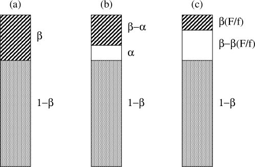
Figure 1: (a) The standard scheme where a predator-prey pair interaction results in either the removal of the prey with probability $\beta$ (striped area) or the exchange of positions with probability $1-\beta$ (gray area). (b) In its habitat an individual from species 1 has a probability $\alpha$ (with $0<\alpha\leq\beta$) to remain unharmed when attacked by a predator (white area: no update to the system) or a probability $\beta-\alpha$ for being removed. (c) The efficiency $f$ respectively $F$ provided to the prey respectively predator results for the case $F<f$ in a non-zero probability $\beta-\beta\left(F/f\right)$ for the prey to survive the attack of the predator and to remain on the same lattice site.

The $(N,r)$ reaction scheme yields a variety of situations, depending on the values of $N$ and $r$. In this work we are interested in situations that lead to the spontaneous formation of spirals where each propagating wave front is dominated by individuals of one species. The two cases we will discuss in detail in the following are the (3,1) case, which is identical to the celebrated May-Leonard model (May and Leonard, 1975; Frey, 2010; Dobramysl et al., 2018), and the (6,4) case (Roman et al., 2013), a game where six species interact in such a way that for each species there is exactly one other species that is not its prey. In a two-dimensional lattice both interaction schemes result in the spontaneous formation of spiral waves. Each spiral arm is dominated by one species, with the following spiral arm containing mainly individuals of the species that is not prey of the first one.

In many studies it is assumed that reaction rates are homogeneous in space and time and also the same for every species. While it is important to consider the simplest version of a model for gaining an understanding of its properties, a more refined approach is needed in order to increase the realism of the model. We consider in the following two modifications of the standard $(N,r)$ model on a lattice, as we add a habitat structure that gives one of the species an advantage in escaping predation, and provide each individual at its birth with a fitness (efficiency) that changes the probability that the prey survives the attack of a predator. We do not change the rate associated with the mobility and the birth rate, keeping them for every individual and at all times at fixed values $\beta$ and $1-\beta$, respectively. The modifications discussed below only affect the rate at which a prey is removed during a predator-prey interaction. In this way we not only minimize the number of free parameters in our model, we also make sure that we only compare situations with a very similar width of the spiral structure, as this width depends strongly on the mobility of the individuals (Reichenbach et al., 2007a).

We divide our lattice in 16 even squares where 8 of them, arranged in a checkerboard, are the habitats of species 1 and provide this species with an advantage evading the attacks of its predators. Whereas in the 8 outside areas all species are equal and interact with the same rate $\beta$, see equations (1)-(3) and Figure 1(a), inside their habitats individuals of species 1 have a reduced probability to be removed when attacked by a predator. As shown in Figure 1(b), this is realized by changing for a prey belonging to species 1 the probability for being removed to $\beta-\alpha$ where the habitat modifier $\alpha$ has a fixed value chosen before the beginning of the simulation from the interval $\left[0,\beta\right]$. It follows that for each attack on a individual of species 1 there is the probability $\alpha$ that the individual escapes unharmed, resulting in no changes to the system. This setup strongly differs from the metapopulation model for the rock-paper-scissors game presented in recent papers (Nagatani et al., 2018a, b) as well as from earlier studies of the May-Leonard model with spatially variable random rates (He et al., 2010, 2011).

Of course, some limiting cases are immediately obtained. For $\alpha=0$ we recover the standard model, whereas for $\alpha=\beta$ species 1 is perfectly safe in its habitats and no attack on an individual from that species will be successful.

In order to make our particle-based description more realistic, we introduce individual fitness and evolutionary adaptation by endowing every individual with a number $f$ that reflects the varying efficiency of their predation and escape capabilities. Our setup follows general ideas introduced in (Dobramysl and Täuber, 2013; Chen et al., 2018) for predator-prey systems with one or two predators, but differs in the details of the implementation. This efficiency is assigned to an individual at its birth (or at the beginning of the simulation in case the individual is present when starting the run). Individuals inherit their efficiency from their parent, but we allow for some random changes that reflect differentiation and adaptation due to mutations. This is realized by generating the efficiency of the off-spring from a Gaussian distribution with variance 1 centered at the efficiency of the parent. When setting up the system we assign a common efficiency $f_{init}$ to all individuals present at the start of the simulation. As we do not change the width of the distribution, it is through the value of $f_{init}$ that we control the relative change of the efficiency at the birth of an off-spring, i.e. for small values of $f_{init}$ the relative change is large, whereas for large values of $f_{init}$ the relative change is small. The case of an efficiency that does not change over time is recovered in the limiting case $f_{init}\longrightarrow\infty$.

Let us denote as $f$ respectively $F$ the efficiencies of the prey respectively the predator that have been selected for an interaction. If the prey is from a species different than species 1 or is a member of species 1 that is not inside one of its habitats, then the probability that the prey is removed is changed to $\beta\left(F/f\right)$ when $F<f$, i.e. because of the larger efficiency of the prey there is the non-zero probability $\beta-\beta\left(F/f\right)$ for the prey to survive the attack of the predator and to remain on its lattice site, see Figure 1(c). For $F>f$ the standard scheme Figure 1(a) prevails where predator and prey are swapping places with probability $1-\beta$ and the prey is removed with probability $\beta$. On the other hand, if the prey is a member of species 1 located in its habitat, then we have the interesting situation that, depending on the value of the ratio $F/f$, either the ability of the prey to escape its attacker is further increased (for $F/f<1$) or the efficiency of the predator reduces the odds of the prey to remain unharmed (for $F/f>1$). Indeed, in the first case the combination of the habitat advantage and the larger efficiency of the prey increases the prey’s probability to survive the attack unharmed to $\mbox{min}\left[\alpha+\beta-\beta\left(F/f\right),\beta\right]$. In the second case, however, the efficiency of the predator works against the advantage of the prey of being in its habitat, which reduces the probability of surviving the attack to $\mbox{max}\left[\alpha+\beta-\beta\left(F/f\right),0\right]$.

In our agent-based simulations we prepare the system initially in a disordered state where with probability $\frac{1}{N+1}$ every lattice site is either occupied by a member of one of the $N$ species or is left empty. We then select randomly a lattice site and one of its four nearest neighbors. In the standard setup, i.e. without habitats and fitness, if the two selected sites are occupied by individuals from two species that have a predator-prey relationship and if the first selected site is occupied by a predator, then with probability $\beta$ the prey is removed from the other lattice site, whereas with probability $1-\beta$ predator and prey swap places. If on the other hand the species involved have a neutral relationship, i.e. do not have a predator-prey relationship, or if the first selected site is not occupied by a predator, then only the swapping takes place with probability $1-\beta$. For the case that exactly one of the selected sites is unoccupied, then the individual located on the occupied site jumps with probability $1-\beta$ into the open site, otherwise it deposits an offspring into this unoccupied lattice site. In the modified versions with habitats and/or fitness, we keep $\beta$ constant, but modify the probability of a successful attack as described above. For all the simulations presented in this work we fixed $\beta=0.3$

We define as one time step $L\times L$ proposed updates that start with a randomly selected site, with $L$ being the linear size of the system. The system sizes discussed in the following range from $L=16$ to $L=56$.

The focus on our work is on the time evolution of the system and on extinction events. In order to obtain data that allow us to discuss probability distributions, for every set of parameters (system size $L$, habitat modifier $\alpha$, initial fitness $f_{init}$) we perform millions of runs with different random initial conditions and different random number sequences.

3 The three-species case

The influence of spatial degrees of freedom and mobility on species evolution and ecosystem self-organization is well established (Turing, 1952; Koch and Meinhardt, 1994; Levin and Segel, 1976; Hassel et al., 1994; Maron and Harrison, 1997; Weber et al., 2014). Cyclic competition between species has been discussed as one possible mechanism responsible for persistent species coexistence. In (Kerr et al., 2002) it was shown that in a spatial setting (i.e. a Petri dish) three cyclically competing strains of bacteria coexist for a long time, whereas in the well-mixed environment of shaken flasks two species go extinct quickly. Both theoretical (Reichenbach et al., 2007a, b, 2008; He et al., 2011; Lamouroux et al., 2012; Rulands et al., 2013; Szczesny et al., 2013, 2014; Szolnoki et al., 2014; Dobramysl et al., 2018) and experimental (Siegert and Weijer, 1995; Igoshin et al., 2004) studies have revealed that spatio-temporal patterns, as for example propagating fronts or spiral waves, often accompany long-lasting coexistence between different species.

As in finite systems fluctuations ultimately yield species extinction, it has been proposed that the dependence of the characteristic extinction time $\tau$ on the system size allows to probe the stability of a system (Antal and Scheuring, 2006; Reichenbach et al., 2007a; Reichenbach and Frey, 2008). In our systems with $L^{2}$ sites the following three scenarios are possible: if $\tau/L^{2}\longrightarrow\infty$ for $L^{2}\longrightarrow\infty$, coexistence is stable and extinction takes very long, whereas if $\tau/L^{2}\longrightarrow 0$ for $L^{2}\longrightarrow\infty$, coexistence is unstable, extinction is fast, and the probability for species extinction taking place approaches 1. These two cases are separated by the case of neutral stability for which $\tau\sim L^{2}$.

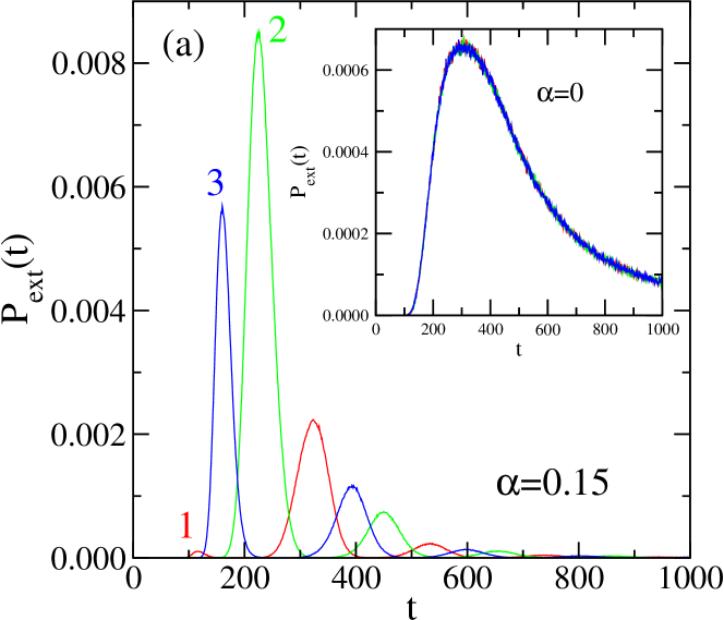
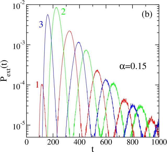
Figure 2: (a) Time-dependent extinction probability for each of the three species in systems with $48\times 48$ sites. The main figure shows the case of habitats where species 1 has an advantage (indicated by the probability $\alpha=0.15$ of surviving attacks from its predator species 3), whereas the inset shows the standard case where all species are treated equally (with $\alpha=0$). To obtain these probability distributions 10 million independent runs were performed for every value of $\alpha$. Red: species 1, green: species 2, blue: species 3. (b) The case $\alpha=0.15$ in a linear-log plot highlighting the periodicity of the peaks in the probability distributions.

3.1 Habitat

For the spatial three-species cyclic game it was shown that spatial heterogeneity in the form of quenched disorder in the reaction rates does not change qualitatively species coexistence and extinction and has only a minor quantitative impact on quantities like the typical extinction time (He et al., 2010, 2011). As we show in the following a spatial heterogeneity in the form of a structured habitat has a much more profound impact on the properties of systems with cyclic dominance.

In Figure 2a we compare for a system of $48\times 48$ sites the time-dependent extinction probabilities for the standard case (inset) as well as for the case $\alpha=0.15$ where inside the habitats species 1 has a major advantage that allows its members to escape an attack unharmed with higher probability. Obviously, for the standard case (the case $\alpha=0$ in the inset) there is no difference between the species, and this is reflected by the probability distributions being the same for the three species. For our system of $48\times 48$ sites and system parameters that take on the values discussed above it takes around 100 time steps after preparation of the system before extinction events show up. For $\alpha=0$ the extinction probability increases until $t\approx 300$ when it reaches a maximum. This time of maximal extinction probability is related to the time the system needs to get organized and form stable space-time patterns. Once these patterns have formed, the extinction probability decreases and displays an algebraic decay $P_{ext}\sim t^{-\beta}$ with $\beta\approx 2.4$. In presence of habitats the probability distributions are strikingly different, as can be seen in the main panel of Figure 2a. While species-dependent extinction probabilities are expected, the observation of multiple maxima in these probabilities is remarkable. These repeated maxima indicate that every species is going periodically through phases where it is susceptible to die out, followed by phases where it is safe from extinction. These successive maxima, which for the parameters used in Figure 2 are separated by 206 time steps, are readily visible in the linear-log plot shown in Figure 2b. This unexpected behavior goes hand in hand with a higher probability of early extinction. Indeed, for $\alpha=0.15$, 99.2% of all runs see a species going extinct before $t=1000$, whereas for the standard case $\alpha=0$ species extinction takes place before $t=1000$ in only 83.1% of the runs.

Periodic oscillations with the same periods as in Figure 2 are also showing up in the time-dependent (average) population densities $x_{i}(t)$ where $i=1,2,3$ labels the three species. This is shown in Figure 3 for a subset of runs that are characterized by the same extinction event (species 2 goes extinct) at the same time ($t=460$) since preparation of the system. Note that the minima in the average population density correspond to the maxima in the extinction probability, as it is most likely that noise drives a species to extinction when the number of individuals of that species is low. Figure 3 also reveals differences in the population densities inside (full lines) and outside (dashed lines) of the habitats that give an advantage to species 1. Whereas one can find more members of species 1 inside the habitats than outside, it is the opposite for species 2, the prey of predator species 1, while the situation is more complicated for species 3 as it depends on time whether the majority of its members can be found inside or outside of these habitats.

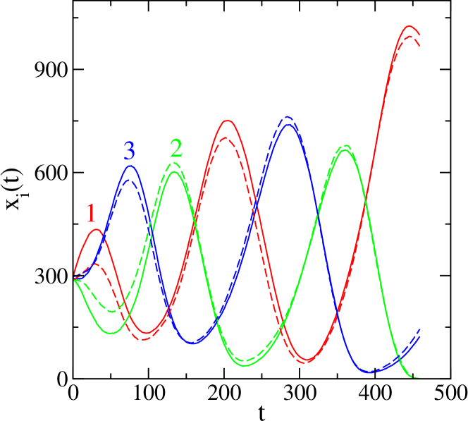
Figure 3: Time evolution of the population density $x_{i}$ of species $i$ ($i=1,2,3$) both inside the habitats that favor species 1 (full lines) as well outside these habitats (dashed lines). The number of sites is $48\times 48$ and $\alpha=0.15$. These data result from averaging over 100 runs for which species 2 goes extinct at $t=460$. Red: species 1, green: species 2, blue: species 3.

The results discussed so far indicate that a structured habitat has a destabilizing effect on species coexistence and creates periodically a situation conductive for species extinction. As discussed above, it is the presence of spiral waves that enhances the stability of the standard May-Leonard system. In our case the habitats favor locally one of the species and therefore act as sources of disorder. Consequently, and this has been verified by analyzing snapshots, the emerging space-time patterns in the presence of habitats are not given by spiral waves filling the system. Instead, outside the habitats one observes multiple wave fronts that criss cross that space. Once (part of) a front dominated by species 2 enters a habitat, the individuals from that species are quickly disposed by species 1. It is the combination of the wave fronts and the disadvantage species 2 has inside the habitats that yield the oscillations in the population densities and concomitantly the periodic appearance of peaks in the species extinction probabilities.

The destabilizing effect due to a locally uneven treatment is consistent with the recent observation that in an uneven three-species May-Leonard model where one species is a less efficient predator than the others the formation of spiral waves is impeded (Menezes et al., 2019).

We have studied quantitatively the dependence of these features on the linear size of the system $L$ and the probability $\alpha$ that an individual of species 1 escapes a predator when attacked inside its habitat. We first note that the destabilizing effect of the habitat is encountered for any value $\alpha>0$. For a fixed system size the period of the oscillations (the time between successive peaks of the extinction probability for a given species) shows a slight dependence on $\alpha$. For example, for $L=48$, the period increase from 200 for $\alpha=0.08$ to 240 for $\alpha=0.2$. For fixed $\alpha$ a strong increase of the period is observed when increasing the system size.

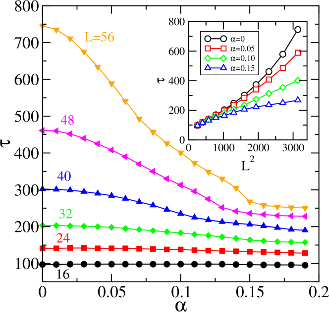
Figure 4: Median extinction time $\tau$ as a function of the habitat modifier $\alpha$ for different linear extents $L$ of the three-species system (ranging from $L=16$ to $L=56$). The inset plots $\tau$ as a function of $L^{2}$ and shows a transition from stable coexistence for small values of $\alpha$ to unstable coexistence for larger values of $\alpha$. For every value of $L$ and $\alpha$ one million runs have been performed. Error bars are smaller than the sizes of the symbols.

With extinction probability distributions like those shown in Figure 2 the mean time to extinction of a species is not a very good measure as it will be dominated by the extremes. Better suited for our purpose is the median extinction time $\tau$ that we show in Figure 4 as a function of $\alpha$ for various values of $L$ and (in the inset) as a function of $L^{2}$ for various values of $\alpha$. Plotting $\tau$ as a function of $\alpha$ reveals for the larger systems different regimes: a first regime for smaller values of $\alpha$ where $\tau$ displays large changes when $\alpha$ is changed, followed by a regime for large $\alpha$ where $\tau$ is largely independent of $\alpha$. Interestingly, changing the value of $\alpha$ induces a qualitative change of the stability of the system, see inset. Whereas for small $\alpha$ coexistence is stable ($\tau/L^{2}$ increases stronger than linear), for $\alpha$ large $\tau/L^{2}$ increases slower than linear and coexistence is unstable. These two regimes are separated by a linear relationship between $\tau$ and $L^{2}$ for $\alpha\approx 0.1$, indicating neutral stability. Thus a structured environment that locally makes the species uneven has a huge impact on biodiversity of an ecology by qualitatively changing the stability of coexistence.

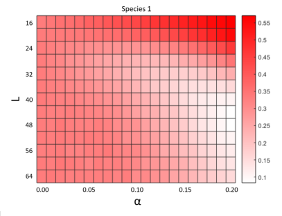
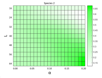
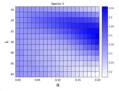
Figure 5: Heatmaps showing the probability as a function of $L$ and $\alpha$ that a species dies out first. For large $\alpha$ and large systems $L$ (lower right corner) species 2 has a very large probability to die out first.

Finally Figure 5 discusses the probability for each species to die out first (the sum of these probabilities being 1). For small values of $\alpha$ the existence of the habitats does not have a pronounced effect on this probability which is still very much the same for all three species. For values of $\alpha$ around 0.1 larger effects start to emerge. The advantage provided by habitats makes it very unlikely for species 1 to die out first for system sizes $L=32$ and larger. This advantage of species 1 is felt strongly by species 2 as this species is pushed to the brink of extinction by their striving predator. More counterintuitive is the observation that in smaller systems it is species 3 that has the highest probability to go extinct first, whereas in the smallest systems species 1 dies out first. This behavior seems to be related to the fact that in systems that are not large enough we do not see the formation of wave fronts, but it is difficult to understand precisely how this changes the chances of a species to vanish.

3.2 Habitat and efficiency

We have also studied whether individual fitness (efficiency), introduced in a way that it contributes to the probability whether an attack of a prey by a predator is successful, impacts extinction probabilities. As discussed above, the efficiency of a parent is inherited by an off-spring, in the sense that the off-spring’s efficiency is drawn from a distribution centered around the parent’s efficiency. The fitness parameter not only determines the efficiency as a predator and a prey, it also allows for evolutionary adaptation.

As we discuss in Figures 6 and 7, including efficiency results in some quantitative changes, but does not modify the general picture discussed previously, namely that the presence of habitats has a destabilizing effect on temporal patterns and a negative impact on species coexistence.

Figure 6: Comparison of the time-dependent extinction probabilities without fitness (dashed lines) and with initial efficiency $f_{init}=10$ (full lines). Other system parameters are $L=48$ and $\alpha=0.15$. These probability distributions are obtained after 10 million independent runs.

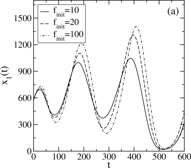
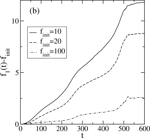
Figure 7: (a) Average time-dependent population density and (b) average time-dependent change in fitness (compared to the initial fitness $f_{init}$) for species 1 obtained from 100 runs that all end at $t=600$ with the extinction of species 3. Other system parameters are $L=48$ and $\alpha=0.15$.

In Figure 6 we compare for $\alpha=0.15$ the extinction probabilities without efficiency (dashed lines) with those where all individuals have been assigned an initial efficiency $f_{init}=10$. We observe a shift to larger times for the maxima in the extinction probabilities as well as an increase of the time elapsed between successive maxima for the same species. These changes can be traced back to the increase over time of the fitness within the different species.

Figure 7 shows time-dependent data obtained for different initial efficiencies $f_{init}$. We remind the reader that the relative change of efficiency between a parent and an off-spring is larger for smaller parent fitness and that the case without fitness discussed in the previous subsection is recovered in the limit $f_{init}\longrightarrow\infty$. With that in mind we show in Figure 7 the time-dependent population density and the time-dependent fitness for species 1 for runs where species 3 dies out after 600 time steps. Changing the value of $f_{init}$ only yields quantitative changes, but has otherwise a negligible effect on biodiversity and species extinction. Inspection of the two panels in Figure 7 reveals that the overall fitness of a species displays pronounced changes at times when the population density decreases. Whenever a species is under pressure from its predator, the most efficient individuals (in terms of escaping a predator and catching a prey) persist and produce off-springs that inherit their increased efficiency.

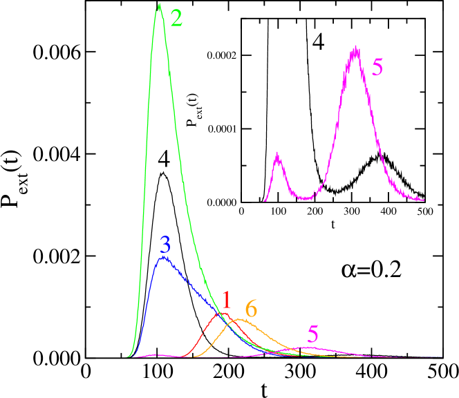
Figure 8: Time-dependent extinction probability for each of the species in the six-species system with $48\times 48$ sites and $\alpha=0.2$. To obtain these probability distributions 10 million independent runs were performed. The inset highlights the existence of multiple peaks in the extinction probabilities of species 4 and 5.

4 The six-species case

In order to check whether the observed destabilizing effect of a structured habitat is generic we extend our study to a six-species case that in the spatially homogeneous system also exhibits spiral waves. Whereas the origin of the spirals in the (6,4) system is the same as for the May-Leonard model (individuals of a given species spontaneously arrange in a wave front that follows a front composed of individuals of the one species that is not a prey of the first one), but there are additional predator-prey relationships between the six species that makes this a more involved case.

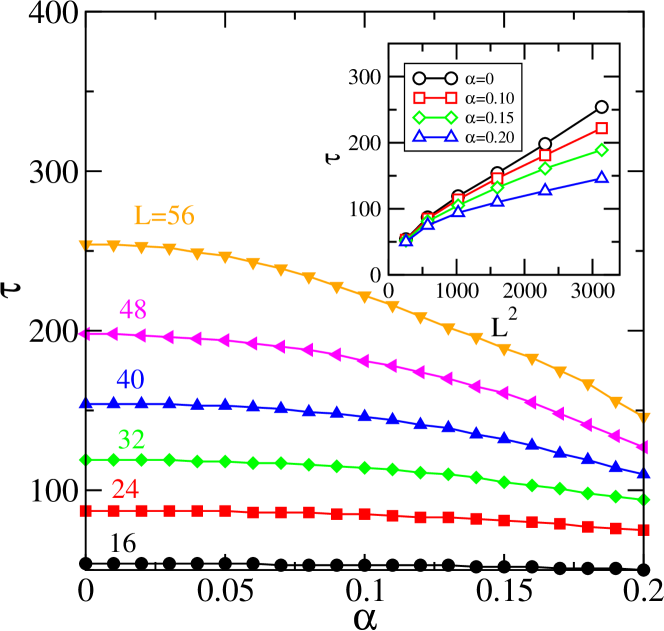
Figure 9: Median extinction time $\tau$ as a function of the habitat modifier $\alpha$ for different linear extents $L$ of the six-species system (ranging from $L=16$ to $L=56$). The inset plots $\tau$ as a function of $L^{2}$ and shows a transition from stable coexistence for small values of $\alpha$ to unstable coexistence for larger values of $\alpha$. For every value of $L$ and $\alpha$, one million runs have been performed. Error bars are smaller than the sizes of the symbols.

Inspection of the extinction probabilities as a function of time reveals that in the six-species system with habitats, that provide an advantage to species 1 through a higher probability to survive unharmed an attack by a predator, the main features observed in the three-species case are also observed. This is shown in Figure 8 for the case $\alpha=0.20$ and $L=48$. As for the three species case the extinction probabilities are different for different species and exhibit a much more complicated dependence on time as for the homogeneous case $\alpha=0$ which has again only one broad maximum followed by a power-law decay, similar to the extinction probabilities for the May-Leonard model shown in the inset of Figure 2a. The inset in Fig. 8 zooms in on the extinction probabilities of two species and shows the presence of more than one peak in the probability distributions. The data are consistent with maxima that are separated by constant time intervals, but our computer resources do not allow us to perform a similar quantitative study of the periodically increasing extinction probabilities as we did for the three-species case.

As before the destabilizing effect of the habitat structure not only yields periodically enhancement of extinction probabilities, it also changes the median time $\tau$ for an extinction event to occur. Plotting $\tau$ as a function of $\alpha$ for fixed $L$ and as a function of $L^{2}$ for fixed $\alpha$, see Figure 9, shows the same trends, albeit not as pronounced, as shown in Figure 4 for the three-species case. From the largest system sizes shown in the inset of Figure 9 it follows that the median extinction time again reveals a transition from stable coexistence for $\alpha$ close to zero to unstable coexistence for larger values of $\alpha$.

While we observe the same effects in presence of habitats for three and six species, the effects are less pronounced for the six-species case. The reason for this can be traced back to the fact that in a homogeneous environment larger systems are needed for the six-species model to form spiral waves. Still, our data for the six-species case are consistent with those for the three-species case, revealing that habitats that locally make the game uneven have generically a debilitating effect on species coexistence.

Finally, we mention that we also introduced efficiency into our six-species system. As for the three-species case only some quantitative changes (for example minor shifts of peak positions in the extinction probability distributions) are observed.

5 Summary

In this paper we addressed the question whether a heterogeneous spatial environment impacts biodiversity and species extinction in systems characterized by cyclic dominance. Earlier studies for the three-species May-Leonard model focused on quenched spatial disorder and found that this type of heterogeneity results only in small quantitative changes. Especially it was revealed that quenched disorder does not have a notable impact on spiral waves which were found to be robust against this type of perturbations.

In our work we considered a different kind of heterogeneous environment consisting of patches embedded in a matrix. In these patches one of the species has an advantage (in our implementation that species has a higher probability to escape unharmed an attack from a predator), whereas in the rest of the system all species are treated equally. Our investigation of two different systems with cyclic dominance and formation of spiral waves (one being a three-species system, whereas the other is formed by six species) shows that the structured habitat has a major impact on the observed space-time patterns. Indeed, in this environment well formed spiral waves do no fill the system, but instead are replaced by wave fronts criss crossing the space outside the habitats. This behavior is facilitated by the fact that if a wave front enters one of the habitats, prey of species 1 are quickly removed. This leads to notable changes to the species extinction probabilities as well as to the median time to extinction, resulting in a transition between stable coexistence and unstable coexistence.

We also studied how fitness and evolutionary adaptation impacts our systems. For every individual we introduce fitness through a parameter that impinges on how this individual fares in a predator-prey interaction. In general a species sees a pronounced increase of its average efficiency in situations where it is under pressure and its population is decreasing. Fitness does however not change dramatically species coexistence and has only a quantitative effect on extinction times.

Whereas we understand well how a habitat impacts a system with cyclic dominance that form spiral patterns in an homogeneous environment, it is an open question whether similar effects are observed in other situations characterized by other types of space-time patterns. We plan to address this question in the future.

References

- Antal and Scheuring (2006) Antal, T., Scheuring, I., 2006. Fixation of strategies for an evolutionary game in finite populations. Bull. Math. Biol. 68, 1923.
- Avelino et al. (2012a) Avelino, P. P., Bazeia, D., Losano, L., Menezes, J., 2012a. von Neummann’s and related scaling laws in rock-paper-scissors-type games. Phys. Rev. E 86 031119.
- Avelino et al. (2012b) Avelino, P. P., Bazeia, D., Losano, L., Menezes, J., de Oliveira, B. F., 2012b. Junctions and spiral patterns in generalized rock-paper-scissors models. Phys. Rev. E 86, 036112.
- Avelino et al. (2014a) Avelino, P. P., Bazeia, Menezes, J., de Oliveira, B. F., 2014a. String networks in Lotka-Volterra competition models. Phys. Lett. A 378, 393.
- Avelino et al. (2014b) Avelino, P. P., Bazeia, D., Losano, L., Menezes, J., de Oliveira, B. F., 2014b. Interfaces with internal structures in generalized rock-paper-scissors models. Phys. Rev. E 89, 042710.
- Avelino et al. (2017) Avelino, P. P., Bazeia, D., Losano, L., Menezes, J., de Oliveira, B. F., 2017. String networks with junctions in competition models. Phys. Lett. A 381, 1014.
- Avelino et al. (2018) Avelino, P. P., Bazeia, D., Losano, L., Menezes, J., de Oliveira, B. F., 2018. Spatial patterns and biodiversity in off-lattice simulations of a cyclic three-species Lotka-Volterra model. EPL (Europhys. Lett.) 121, 48003.
- Avelino et al. (2019) Avelino, P. P., Menezes, J., de Oliveira, B. F., Pereira, T. A., 2019. Domain expansion and transient scaling regimes in population networks with in-domain cyclic selection. arXiv:1811.07412.
- Brown and Pleimling (2017) Brown, B. L., Pleimling, M., 2017. Coarsening with non-trivial in-domain dynamics: correlations and interface fluctuations. Phys. Rev. E 96, 012147.
- Brown et al. (2019) Brown, B. L., Meyer-Ortmanns, H., Pleimling, M., 2019. Dynamically generated hierarchies in games of competition. Phys. Rev. E 99, 062116.
- Chen et al. (2018) Chen, S., Dobramysl, U., Täuber, U.C., 2018. Evolutionary dynamics and competition stabilize three-species predator-prey communities. Ecological Complexity 36, 57.
- Cheng et al. (2014) Cheng, H., Yao, N., Huang, Z. G., Park, J., Do, Y., Lai, Y. C., 2014. Mesoscopic interactions and species coexistence in evolutionary game dynamics of cyclic competitions. Sci. Rep. 4, 7486.
- Danku et al. (2018) Danku, Z., Wang, Z., Szolnoki, A., 2018. Imitate or innovate: Competition of strategy updating attitudes in spatial social dilemma games. EPL (Europhys. Lett.) 121, 18002.
- Dobramysl et al. (2018) Dobramysl, U., Mobilia, M., Pleimling, M., Täuber, U.C., 2018. Stochastic population dynamics in spatially extended predator-prey systems. J. Phys. A: Math. Theor. 51, 063001.
- Dobramysl and Täuber (2013) Dobramysl, U., Täuber, U.C., 2013. Environmental versus demographic variability in two-species predator-prey models Phys. Rev. Lett. 110, 048105.
- Esmaeili et. al. (2018) Esmaeili, S., Brown, B.L., Pleimling, M., 2018. Perturbing cyclic predator-prey systems: how a six-species coarsening system with non-trivial in-domain dynamics responds to sudden changes. Phys. Rev. E 98, 062105.
- Frey (2010) Frey, E., 2010. Evolutionary game theory: Theoretical concepts and applications to microbial communities. Physica A 389, 4265.
- Hassel et al. (1994) Hassel, M. P., Comins, H. N., May, R. M., 1994. Species coexistence and self-organizing spatial dynamics. Nature 370, 290.
- He et al. (2010) He, Q., Mobilia, M., Täuber U.C., 2010. Spatial rock-paper-scissors models with inhomogeneous reaction rates. Phys. Rev. E 82, 051909.
- He et al. (2011) He, Q., Mobilia, M., Täuber U.C., 2011. Coexistence in the two-dimensional May-Leonard model with random rates. Eur. Phys. J. B 82, 97.
- Hofbauer and Sigmund (1998) Hofbauer, J., Sigmund, K., 1998. Evolutionary games and population dynamics. Cambridge University Press, Cambridge, England.
- Kerr et al. (2002) Kerr, B., Riley, M. A., Feldman, M. W., Bohannan, B. J. M., 2002 Local dispersal promotes biodiversity in a real-life game of rock-paper-scissors. Nature 418, 171.
- Kirkup and Riley (2004) Kirkup, B. C., Riley, M. A., 2004. Antibiotic-mediated antagonism leads to a bacterial game of rock-paper-scissors in vivo. Nature 428, 412.
- Koch and Meinhardt (1994) Koch, A. J., Meinhardt, H., 1994. Biological pattern formation: from basic mechanisms to complex structures. Rev. Mod. Phys 66, 1481.
- Labavić and Meyer-Ortmanns (2016) Labavić, D., Meyer-Ortmanns, H., 2016 Rock-paper-scissors played within competing domains in predator-prey games. J. Stat. Mech. (2016), 113402.
- Lamouroux et al. (2012) Lamouroux, D., Eule, S., Geisel, T., Nagler, J., 2012. Discriminating the effects of spatial extent and population size in cyclic competition among species. Phys. Rev. E 86, 021911.
- Levin and Segel (1976) Levin, S. A., Segel, L. A., 1976. Hypothesis to explain the origin of planktonic patchness. Nature 259, 659.
- Maron and Harrison (1997) Maron, J. L., Harrison, S., 1997. Spatial pattern formation in an insect host-parasitoid system. Science 278, 1619.
- May (1974) May, R. M., 1974. Stability and complexity in model ecosystems. Cambridge University Press, Cambridge, England.
- May and Leonard (1975) May, R.M., Leonard, W., 1975. Nonlinear aspects of competition between three species. SIAM J. Appl. Math. 29, 243.
- Maynard Smith (1974) Maynard Smith, J., 1974. Models in ecology. Cambridge University Press, Cambridge, England.
- Maynard Smith (1982) Maynard Smith, J., 1982. Evolution and the theory of games. Cambridge University Press, Cambridge, England.
- Menezes et al. (2019) Menezes, J., Moura, B., Pereira, T. A., 2019. Uneven rock-paper-scissors models: Patterns and coexistence. EPL (Europhys. Lett.) 126, 18003.
- Mowlaei et al. (2014) Mowlaei, S., Roman, A., Pleimling, M., 2014. Spirals and coarsening patterns in the competition of many species: A complex Ginzburg-Landau approach. J. Phys. A: Math. Theor. 47, 165001.
- Nagatani et al. (2018a) Nagatani, T., Tainaka, K., Ichinose, G., 2018a. Metapopulation model of rock-scissors-paper game with subpopulation-specific victory rates stabilized by heterogeneity. J. Theor. Biol. 458, 103.
- Nagatani et al. (2018b) Nagatani, T., Ichinose, G., Tainaka, K., 2018b. Heterogeneous network promotes species coexistence: metapopulation model for rock-paper-scissors game. Sci. Rep. 8, 7094.
- Nowak (2006) Nowak, M. A., 2006. Evolutionary dynamics. Belknap Press, Cambridge, MA.
- Perc et al. (2007) Perc, M., Szolnoki, A., Szabó, G., 2007. Cyclical interactions with alliance-specific heterogeneous invasion rates. Phys. Rev. E 75, 052102.
- Reichenbach et al. (2007a) Reichenbach, T., Mobilia, M., Frey, E., 2007a. Mobility promotes and jeopardizes biodiversity in rock-paper-scissors games. Nature 448, 1046.
- Reichenbach et al. (2007b) Reichenbach, T., Mobilia, M., Frey, E., 2007b. Noise and correlations in a spatial population model with cyclic competititon. Phys. Rev. Lett. 99, 238105.
- Reichenbach et al. (2008) Reichenbach, T., Mobilia, M., Frey, E., 2008. Self-organization of mobile populations in cyclic competititon. J. Theor. Biol. 254, 368.
- Reichenbach and Frey (2008) Reichenbach, T., Frey, E., 2008. Instability of spatial patterns and its ambiguous impact on species diversity. Phys. Rev. Lett. 101, 058102.
- Roman et al. (2012) Roman, A., Konrad, D., Pleimling, M., 2012. Cyclic competition of four species: domains and interfaces. J. Stat. Mech. (2012), P07014.
- Roman et al. (2013) Roman, A., Dasgupta, D., Pleimling, M., 2013. Interplay between partnership formation and competition in generalized May-Leonard games. Phys. Rev. E 87, 032148.
- Roman et al. (2016) Roman, A., Dasgupta, D., Pleimling, M., 2016. A theoretical approach to understand spatial organization in complex ecologies. J. Theor. Biol. 403, 10.
- Rulands et al. (2013) Rulands, S., Zielinski, A., Frey, E., 2013. Global attractors and extinction dynamics of cyclically competing species. Phys. Rev. E 87, 052710.
- Siegert and Weijer (1995) Siegret G., Weijer, C. J., 1995. Spiral and concentric waves organize multicellular Dictyostelium mounds. Curr. Biol. 5, 937.
- Igoshin et al. (2004) Igoshin, O. A., Welch, R., Kaiser, D., Oster, G., 2004. A biochemical oscillator explains several aspects of Myxococcus xanthus behavior during development. Proc. Natl. Acad. Sci. U.S.A 101, 15760.
- Szabó and Czárán (2001a) Szabó, G., Czárán, T., 2001a. Phase transition in a spatial Lotka-Volterra model. Phys. Rev. E 63, 061904.
- Szabó and Czárán (2001b) Szabó, G., Czárán, T., 2001b. Defensive alliances in spatial models of cyclical population interactions. Phys. Rev. E 64, 042902.
- Szabó and Sznaider (2004) Szabó, G., Sznaider, G. A., 2004. Phase transition and selection in a four-species cyclic predator-prey model. Phys. Rev. E 69, 031911.
- Szabó (2005) Szabó, G., 2005. Competing associations in six-species predator-prey models. J. Phys. A: Math. Gen. 38, 6689.
- Szabó and Fáth (2007) Szabó, G., Fáth, G., 2007. Evolutionary games on graphs. Phys. Rep. 446, 97.
- Szabó et al. (2007a) Szabó, G., Szolnoki, A., Sznaider, G. A., 2007a. Segregation process and phase transition in cyclic predator-prey models with an even number of species. Phys. Rev. E 76, 051921.
- Szabó et al. (2007b) Szabó, P., Czárán, T., Szabó, G., 2007b. Competing associations in bacterial warfare with two toxins. J. Theor. Biol. 248, 736.
- Szabó and Szolnoki (2008) Szabó, G., Szolnoki, A., 2008. Phase transitions induced by variation of invasion rates in spatial cyclic predator-prey models with four or six species. Phys. Rev. E 77, 011906.
- Szabó et al. (2008) Szabó, G., Szolnoki, A., Borsos, I., 2008. Self-organizing patterns maintained by competing associations in a six-species predator-prey model. Phys. Rev. E 77, 041919.
- Szczesny et al. (2013) Szczesny, B., Mobilia, M., Rucklidge, A. M., 2013. When does cyclic dominance lead to stable spiral waves? EPL (Europhys. Lett.) 102, 28012.
- Szczesny et al. (2014) Szczesny, B., Mobilia, M., Rucklidge, A. M., 2014. Characterization of spiraling patterns in spatial rock-paper-scissors games. Phys. Rev. E 90, 032704.
- Szolnoki et al. (2014) Szolnoki, A., Mobilia, M., Jiang, L. L., Szczesny, B., Rucklidge, A. M., Perc, M., 2014. Cyclic dominance in evolutionary games: a review. J. Roy. Soc. Interface 11, 20140735.
- Szolnoki and Perc (2015) Szolnoki, A., Perc, M., 2015. Reentrant phase transitions and defensive alliances in social dilemmas with informed strategies. EPL (Europhys. Lett.) 110, 38003.
- Szolnoki and Perc (2018) Szolnoki, A., Perc, M., 2018. Evolutionary dynamics of cooperation in neutral populations. New. J. Phys. 20, 013031.
- Turing (1952) Turing, A. M., 1952. The chemical basis of morphogenesis. Phil. Trans. R. Soc. B 237, 37.
- Weber et al. (2014) Weber, M. F., Poxleitner, G., Hebisch, E., Frey, E., Opitz, M., 2014. Chemical warfare and survival strategies in bacterial range expansions. J. R. Soc. Interface 11, 20140172.
- Vukov et al. (2013) Vukov, J., Szolnoki, A., Szabó, G., 2013. Diverging fluctuations in a spatial five-species cyclic dominance game. Phys. Rev. E 88, 022123.