Consensus-based Optimization for 3D Human Pose Estimation in Camera Coordinates

Abstract

3D human pose estimation is frequently seen as the task of estimating 3D poses relative to the root body joint. Alternatively, we propose a 3D human pose estimation method in camera coordinates, which allows effective combination of 2D annotated data and 3D poses and a straightforward multi-view generalization. To that end, we cast the problem as a view frustum space pose estimation, where absolute depth prediction and joint relative depth estimations are disentangled. Final 3D predictions are obtained in camera coordinates by the inverse camera projection. Based on this, we also present a consensus-based optimization algorithm for multi-view predictions from uncalibrated images, which requires a single monocular training procedure. Although our method is indirectly tied to the training camera intrinsics, it still converges for cameras with different intrinsic parameters, resulting in coherent estimations up to a scale factor. Our method improves the state of the art on well known 3D human pose datasets, reducing the prediction error by 32% in the most common benchmark. We also reported our results in absolute pose position error, achieving 80 mm for monocular estimations and 51 mm for multi-view, on average. Source code is available at https://github.com/dluvizon/3d-pose-consensus.

1 Introduction

3D human pose estimation is a very active research topic, mainly due to the several applications that benefit from precise human poses, such as sports performance analysis, 3D model fitting, human behavior understanding, among many others. Despite the recent works on 3D human pose estimation, most of the methods in the literature are limited to the problem of relative pose prediction [8, 49, 61, 4, 2], where the root body joint is centered at the origin and the remaining joints are estimated relative to the center. This limitation hinders the generalization for multi-view scenarios since predictions are not in the camera coordinates. Contrarily, when estimations are relative to a static referential, predictions can be easily projected from one view to another, as illustrated in Fig. 1.

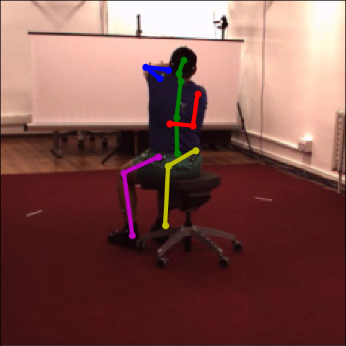
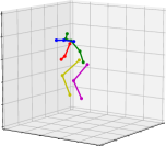
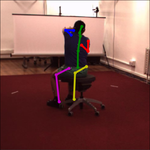
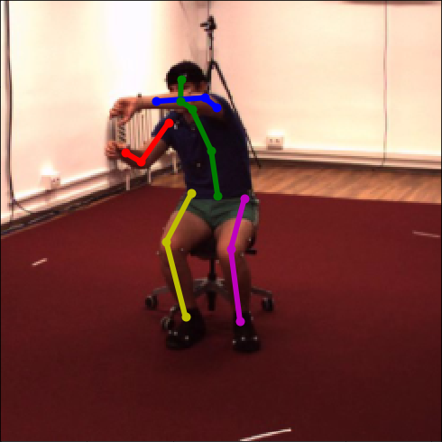
Figure 1: Absolute 3D human pose estimated from a single image (top-left) with occlusion and projected into a different view (top-right). Our multi-view consensus-based approach (bottom) results in a more precise absolute pose estimation and effectively handles cases of occlusion.

The methods in the state of the art frequently handle 3D human pose estimation as a regression task, directly converting the input images to predicted poses in millimeters [47, 24]. However, this is a depth learning problem, because identical distances in pixels can result in different distances in millimeters. For example, a person close to the camera with the hand next to the head has a distance (head to hand in mm) much shorter than a person far from the camera with her arm extended, although both result in the same distance in pixels. Consequently, those methods have to learn the intrinsic parameters indirectly. Moreover, by predicting 3D poses directly in millimeters, the abundant images with annotated 2D poses in pixels cannot be easily exploited, since this data has no associated 3D information, and relative poses predicted from one camera cannot be easily projected into a different view, making it more difficult to handle occlusion cases in multi-view scenarios.

In our method, we tackle these limitations by casting the problem of 3D human pose estimation into a different perspective: instead of directly predicting pose in millimeters relative to the root joint, we predict 3D poses in the view frustum space, i.e., we predict $(u,v)$ coordinates in the image plane, in pixels, and the absolute depth in millimeters. We further split depth estimation as a global absolute depth and joint relative depth estimations. Both 2D human pose and absolute depth estimation are well known problems in the literature [3, 11, 9, 22], including absolute depth estimation benchmarks [33, 53], but are usually not correlated. In our method, we train a feed-forward neural network by effectively merging in-the-wild 2D data and precise 3D poses, making the best use of each. Even though our network is trained only with monocular images, the predictions from individual views can be merged by the proposed consensus-based optimization in order to produce multi-view estimations, resulting in an effective way to handle the challenging cases of occlusions, as demonstrated by a significant improvement in accuracy in our experiments. Although our training scheme is indirectly tied to the camera intrinsics, our method has demonstrated a generalization capability to predict 3D poses up to a scale from a completely different camera setup, including different intrinsic parameters. This was evidenced by qualitative and quantitative evaluations.

Considering the exposed limitations of relative 3D human pose estimation, we aim to fill the gap of current methods by addressing the more complex problem of absolute 3D human pose estimation, where predictions are performed with respect to a static referential i.e., the camera position, and not to the person’s root joint. In that direction, we present our contributions: First, we propose an absolute 3D human pose estimation method from monocular cameras which achieves results in the state of the art when considering similar camera intrinsics at training and inference time. Second, we propose a consensus-based optimization for multi-view absolute 3D human pose estimation from uncalibrated images, which requires a single monocular training procedure. The multi-view estimation approach is capable of generalizing for different camera setups, resulting in coherent 3D absolute predictions up to a scale factor. Our method sets the new state-of-the-art results on the challenging test set from Human3.6M, improving previous results by 10% with monocular predictions and by 32% considering multiple views.

The remaining of this paper is divided as follows. In section 2 we present the related work. Our method for 3D human pose estimation is explained in section 3 and our algorithm for consensus-based optimization is detailed in section 4. The experiments are presented in section 5 and in section 6 we conclude this paper.

2 Related work

In this section, we review the methods most related to our work, giving special attention to monocular (relative and absolute) and multi-view 3D human pose estimation. We recommend the survey in [44] for readers seeking for a more detailed review.

2.1 Monocular relative 3D human pose estimation

In the last decade, monocular 3D human pose estimation has been a very active research topic in the community [1, 60, 48, 24, 15]. Many recent works have proposed to directly predict relative 3D poses from images [47, 46, 37], which requires the model to learn a complex projection from 2D pixels to millimeters in three dimensions. Another drawback is their limitation to benefit from the abundant 2D data, since manually annotated images have no associated 3D information.

A common approach to directly use 2D data during training is to first learn a 2D pose estimator, than lift 3D poses from 2D estimations [23, 40, 54, 49, 27, 8]. However, lifting 3D from 2D points only is an ill-defined problem since no visual cues are available, frequently resulting in ambiguity and, consequently, limited precision. Other methods assume that the absolute location of the root joint is provided during inference [59, 25], so the inverse projection from pixels to millimeters can be performed. In our approach, this assumptions is not made, since we estimate the 3D pose in absolute coordinates. The only additional information we need are the intrinsic parameters for monocular prediction, which is often given by the manufacturer or could be estimated by standard tools. In addition and differently from [25], our approach allows combining predictions from multiple views of the scene, resulting in more precise estimations.

Contrarily to the previous work, we are able to train our method simultaneously with 3D and 2D annotated data in an effective way, since one part of our prediction is performed in the image plane and completely independent from 3D information. Moreover, estimating the first two coordinates in pixels in the image plane is a better defined problem than estimating floating 3D positions directly in millimeters. These advantages translate into higher accuracy for our method.

2.2 Monocular absolute 3D human pose estimation

Contrarily to relative estimation, in absolute pose prediction the 3D coordinates of the human body are predicted with respect to the camera or in the view frustum space. A simple approach is to infer the distance to the camera considering a normalized or constant body size [61, 30], which is an information that may not be available and difficult to be estimated [12]. Inspired by the many works on depth estimation, Nie et al. [35] predict the depth of body joints individually. The drawback of this method is that it suffers to capture the human body structure, since errors in the estimated depth for individual joints can degenerate the final pose.

More recently, multi-person absolute pose estimation methods were proposed [32, 29]. In [32], the absolute distance from the person to the camera is predicted based on the area of the cropped 2D bounding box. However, it is known from the literature on absolute depth estimation [10, 9] that not only the size of objects are important, but also their positions in the image is an informative cue to predict its depth. For example, a person in the bottom of an image is more likely to be closer to the camera than a person on the top of the same image. Differently, in [29], the authors optimized the person absolute distance based on the initial bone lengths, estimated from the first 10 frames of a video sequence, and on the re-projection of the 3D pose into the 2D body joint locations. Besides this approach relies on video sequences, it also requires the camera parameters.

In our approach, we combine three different information to predict the distance of the root joint w.r.t. the camera position: the size of the bounding box (including its ratio), the target position in the image, and deep convolutional features that provide additional visual cues.

2.3 Multi-view pose estimation and camera calibration

For the challenging cases of occlusion or clutter background, multiple views can be decisive to disambiguate uncertain positions of body joints (see Fig. 1). To handle this, several works have proposed multi-view solutions for 3D human pose estimation [4, 2, 6, 5, 14], mostly exploring the classical concept of pictorial structures from multi-view images. Deep neural networks have been used to estimate relative 3D poses from a set of 2D predictions from different views [42, 38, 36]. As an example, Pavlakos et al. [38] proposed to collect 3D poses from 2D multi-view image, which are used to learn a second model to perform 3D estimations. Since these methods estimate 3D from multiple 2D images, they often require both intrinsic and extrinsic parameters.

In order to estimate the full camera calibration parameters, Micusik and Pajdla [31] proposed to use a human body seen at different positions in the image. The main limitation of this approach is the fact that it assumes that all poses as nearly vertical and parallel to each other. Considering multiple views of the same person, Rhodin et al. [42] propose to estimate 3D poses from each individual view and to estimate the extrinsic camera calibration, assuming that the intrinsic parameters are provided as input. More recently, Iskakov et al. [17] proposed a learnable triangulation of 3D poses, considering multiple fully calibrated views during training. Despite the impressive results achieved in this work, the network model is training considering a pre-defined camera positioning, which could result in a strong overfiting in the experimental setup. Differently, our model is trained without priors about the camera positions and the proposed multi-view optimization algorithm is not directly tied to a specific camera setup.

From the recent literature, we can notice that current multi-view approaches are still completely dependent on the camera intrinsic parameters and often require a complete calibration setup, which can be prohibitive in some circumstances. Available methods are also limited to the inference of 3D from multiple 2D predictions, requiring multi-view datasets for training. Alternatively, we propose to predict absolute 3D poses from each individual view, which has two important advantages over previous methods. First, it allows us to easily combine predictions from multiple calibrated cameras, while requiring a single monocular training procedure. Second, we are able to estimate camera calibration, both intrinsic and extrinsic, from multi-view images, by a consensus-based optimization without retraining the model. The strength of our approach is evidenced by its strong results, even when considering unknown and uncalibrated cameras.

3 Proposed method for 3D human pose estimation

One of the goals of our method is to predict 3D human poses in absolute coordinates with respect to the camera position. For this, we believe that the most effective approach is to predict each body joint in image pixel coordinates and in absolute depth, orthogonal to the image plane, in millimeters. Then, the predicted pixel coordinates and depth can be projected to the world coordinates, considering a pinhole camera model.

We further split the problem as relative 3D pose estimation and absolute depth estimation. The motivation for this comes from the idea that a well cropped bounding box around the person is better for predicting its pose than the full image frame, since a better resolution could be attained and the person scale is automatically handled by the image crop, although small variations in the bounding boxes during training result in better robustness. Additionally, by providing a separated loss on relative depth for each joint helps the network to learn the human body structure, which would be more difficult to learn directly from absolute coordinates due to position shift.

Recent works on depth estimation have demonstrated that neural networks rely on both pictorial cues and geometry information to predict depth [10]. For the specific problem of 3D human pose estimation, the structure of the human body is also an important domain knowledge to be explored. Considering our motivations and the exposed challenges, we propose to predict 3D poses relative to a cropped region centered at the person, which eases the network to encode the human body structure, and absolute depth from combined local pictorial cues and global position and size of the cropped region.

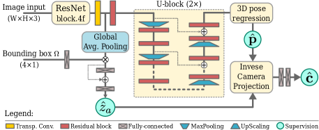
Figure 2: Proposed ResNet-U architecture. A given input image and the corresponding bounding box parameters are fed into a neural network that predicts absolute depth $\hat{\mathit{z}}_{a}{}$, human pose $\hat{\mathbf{p}}{}$, and confidence scores $\hat{\mathbf{c}}{}$.

Specifically, given an image $\mathbf{I}\in\mathbb{R}^{W\times{H}\times{3}}$ and a person bounding box region $\Omega\in\mathbb{R}^{4\times 1}$, we define the problem as learning a function $\mathcal{F}$: $\{\mathbf{I},\Omega\}\xrightarrow[]{\mathcal{F}}~{}\{\hat{\mathbf{p}}{},\hat{\mathbf{c}}{},\hat{\mathit{z}}_{a}{}\}$, where $\hat{\mathbf{p}}{}\in\mathbb{R}^{3\times{J{}}}$ is the estimated relative pose, composed of $J{}$ body joints in the format $(\hat{u}_{i}{},\hat{v}_{i}{},\hat{d}_{i}{})^{T}$, with $i=\{1,\dots,J{}\}$, $\hat{\mathbf{c}}{}\in\mathbb{R}^{1\times J{}}$ contains the body joint confidence score, which is an additional information that represents a level of confidence for each predicted body joint coordinates, and $\hat{\mathit{z}}_{a}{}\in\mathbb{R}_{\geq 0}$ is the estimated absolute depth for the person’s root joint. The person bounding box $\Omega$ is defined by its central position $(x_{\Omega},y_{\Omega})$ and size $(w_{\Omega},h_{\Omega})$, and can be obtained using a standard person detector [41]. The parametrized regression function $\mathcal{F}$ is implemented as a deep convolutional neural network (CNN), detailed as follows.

3.1 Network architecture

U-Nets are widely used for human pose estimation due to their multi-scale processing capability [34], while classic residual networks [13] are often preferable to produce CNN features. Since we want precise pose predictions and informative visual features for absolute depth estimation, our network combines a ResNet-50 model cut at block 4f as backbone and U-blocks, as shown in Fig. 2. This architecture is called ResNet-U and, in addition to a few fully connected layers to regress the absolute depth $\hat{\mathit{z}}_{a}{}$ and the confidence scores $\hat{\mathbf{c}}{}$, implements the function $\mathcal{F}$. The details about each part of our method is discussed as follows.

3.2 3D human pose estimation

As previously stated, we first want to estimate the 3D human pose relative to the cropped bounding box. To this end, we first predict the pixel coordinates $(\hat{u}_{i}{},\hat{v}_{i}{})$ in the image plane, given the information about the cropped image in $\Omega$. Since it is difficult to predict the absolute depth from an arbitrarily cropped region, at this stage we predict the relative depth of each body joint with respect to the location of the person. Therefore, the human pose estimation problem can be naturally split into two parts: relative pose estimation and absolute body joints depth estimation, as detailed next.

3.2.1 Relative human pose estimation

For the pose prediction in the image plane $(u,v)$, we use the soft-argmax operation [26, 55], which induces the U-Nets to generate one probability distribution per body joint. This probability distribution is defined as a feature map $\mathbf{h}{}_{i}\in\mathbb{R}^{w_{f}\times{h_{f}}}$ (positive and unitary sum) for the $i$th body joint. The third dimension of the pose $\hat{\mathbf{p}}{}$ is composed of the depth per body joint, with respect to the location of the person. This prediction could be integrated in the soft-argmax by extending the feature map $\mathbf{h}{}$ to a volumetric representation [47]. However, depending on the resolution and the number of body joints, this approach can be costly. Instead, we predict a normalized depth map $\mathbf{d}{}\in\mathbb{R}^{w_{f}\times{h_{f}}}$ per body joint, corresponding to an interval of 2 meters, which is a common reference size in other methods [37]. By restricting the estimated depth to this range, we ensure that the bounding box prediction is well defined inside an small region, corresponding to the enclosure of an average person. The regressed depth inside the bounding box is defined by:

$$\hat{d}_{i}{}=\lambda\Big{(}\sum_{\mathbf{y}{}=(1,1)}^{(w_{f},h_{f})}d_{i}(\mathbf{y}{})h_{i}(\mathbf{y}{})\Big{)},$$ (1)

where $\lambda$ is a normalization function, $d_{i}(\mathbf{y}{})$ and $h_{i}(\mathbf{y}{})$ are the values of the depth and the joint probability distribution for the $i$th joint at pixel $\mathbf{y}{}$. Note that in Equation 1 the regions in the depth maps are pooled accordingly to the high probability locations of the body joints.

3.2.2 Absolute depth estimation

Once we have estimated the body joint coordinates in pixels and the depth with respect to the location of the person, we then predict the absolute depth of the person with respect to the camera. For this, we use two complementary sources of information: the bounding box information (position and size), and deep visual features. The position and size of the bounding box provide a rough global information about the scale and position of the person in the image. Additionally, the visual features extracted from the bounding box region by means of ResNet features provide informative visual cues that are used to refine the absolute person distance estimation.

Both extracted features are then fed to a fully connected network with 256 neurons at each level and a single neuron as output, represented by $\alpha_{z}$, which is activated by a smoothed sigmoid function, defined as:

$$\hat{\mathit{z}}_{a}{}=\rho\frac{1}{1+e^{\beta\alpha_{z}}},$$ (2)

where $\rho$ is the maximum depth, set as 10 meters in our experiments, and $\beta$ is a smoothing factor, set to 0.5 in our experiments. The output $\hat{\mathit{z}}_{a}{}$ is then supervised with the absolute depth of the root joint $\mathit{z}_{a}$. This process is illustrates in Fig. 2 in the bottom left part. We demonstrated in our experiments that the two different types of information, visual and bounding box information, are complementary for the task of absolute depth prediction.

3.2.3 Absolute 3D human pose reconstruction

In order to accomplish our objective of estimating the absolute 3D pose represented as $\hat{\mathbf{x}}{}=(\hat{x}_{i}{},\hat{y}_{i}{},\hat{z}_{i}{})^{T}$, we combine the estimated pose in the bounding box with the predicted absolute depth. Considering $(\hat{u}_{i}{},\hat{v}_{i}{},\hat{d}_{i}{})^{T}$ as the first and $\hat{\mathit{z}}_{a}{}$ as the last, the absolute $z$ coordinate for each body joint is defined by $\hat{z}_{i}{}=\hat{d}_{i}{}+\hat{\mathit{z}}_{a}{}$. Note that $\hat{z}_{i}{}$ is the absolute distance in millimeters from each body joint to the camera and it results from the combination of two distinct predictions, which are individually supervised. The other two absolute coordinates required to build the final absolute 3D pose, $\hat{x}_{i}{}$ and $\hat{y}_{i}{}$, can then be computed using the pinhole camera model by the following equation:

$$\begin{bmatrix}\hat{x}_{i}{}\\ \hat{y}_{i}{}\end{bmatrix}=\begin{bmatrix}1/f_{x}{}&0&-C_{x}{}/f_{x}{}\ \\ 0&1/f_{y}{}&-C_{y}{}/f_{y}{}\\ \end{bmatrix}\begin{bmatrix}\hat{u}_{i}{}\\ \hat{v}_{i}{}\\ 1\end{bmatrix}\hat{z}_{i}{},$$ (3)

where $f$ and $C$ are the camera focal length and the camera center, both in pixels, considering the $x$ and $y$ axis. Note that these parameters are camera intrinsics and can be easily obtained. The camera focal length is often given by the manufacturer and the center of the image frequently corresponds to the image center in pixels or, even, both values could be estimated with standard tools. Nevertheless, in what follows we present a method to estimate the camera parameters, both intrinsic and extrinsic, without any prior information, directly from the predictions of our method, considering a multi-view scenario with uncalibrated cameras.

4 Consensus-based optimization

One of the main advantages of estimating absolute instead of relative 3D poses is the possibility to project the predictions from one camera to another, simply by applying a rotation and a translation. This advantage has important consequences in multi-view. For example, when the camera calibration is known, the predictions of different monocular cameras can be combined with respect to a common reference, resulting in more precise predictions. For the cases where no information is known about the camera calibration, we propose a consensus-based algorithm that can be applied to estimate both intrinsic and extrinsic parameters, resulting in a completely uncalibrated multi-view approach. This algorithm is explained as follows.

Let us define the predictions of the proposed method from two distinct cameras as: $\hat{\mathbf{p}}{}_{c1}=(\hat{u}_{i}{},\hat{v}_{i}{},\hat{z}_{i}{})_{c1}^{T}$ and $\hat{\mathbf{p}}{}_{c2}=(\hat{u}_{i}{},\hat{v}_{i}{},\hat{z}_{i}{})_{c2}^{T}$, and their poses in absolute camera coordinates: $\hat{\mathbf{x}}{}_{c1}=(\hat{x}_{i}{},\hat{y}_{i}{},\hat{z}_{i}{})_{c1}^{T}$ and $\hat{\mathbf{x}}{}_{c2}=(\hat{x}_{i}{},\hat{y}_{i}{},\hat{z}_{i}{})_{c2}^{T}$, respectively for cameras 1 and 2. Then, we define the projection of $\hat{\mathbf{x}}{}_{c2}$ into camera 1 as:

$$\hat{\mathbf{x}}{}_{c2\rightarrow{c1}}=\textbf{R}_{2,1}(\hat{\mathbf{x}}{}_{c2}-\textbf{T}_{2,1}),$$ (4)

where $\textbf{R}_{2,1}\in\mathbb{R}^{3\times 3}$ and $\textbf{T}_{2,1}\in\mathbb{R}^{3\times 1}$ are a rotation matrix and a translation vector from camera 2 to camera 1. Our goal is to minimize the projection error from camera 2 to camera 1 (and vice-versa) by optimizing a set of camera parameters:
$\textbf{K}_{2,1}\in\{f_{x}{}_{1},f_{y}{}_{1},C_{x}{}_{1},C_{y}{}_{1},f_{x}{}_{2},f_{y}{}_{2},C_{x}{}_{2},C_{y}{}_{2},\textbf{R}_{2,1},\textbf{T}_{2,1}\}$, which includes the intrinsics from both cameras and the extrinsic parameters between them. Specifically, let us define the optimization problem as:

$$\textbf{K}^{\ast}_{2,1}=\operatorname*{arg\,min}_{\textbf{K}_{2,1}}\|\hat{\mathbf{x}}{}_{c1}-\hat{\mathbf{x}}{}_{c2\rightarrow{c1}}\|_{F}^{2}.$$ (5)

We find a solution for Equation 5 by using an optimization approach that sequentially considers the individual variables by alternating gradient with steepest descent. This process is detailed as follows.

4.1 Camera parameters optimization

In order to obtain the translation vector from camera 2 to camera 1 that minimizes Equation 5, we define:

$$\textbf{T}^{\ast}_{2,1}=\operatorname*{arg\,min}_{\textbf{T}_{2,1}}\|\hat{\mathbf{x}}{}_{c1}-\textbf{R}_{2,1}(\hat{\mathbf{x}}{}_{c2}-\textbf{T}_{2,1})\|_{F}^{2}.$$ (6)

By replacing the squared Frobenius norm $\|\mathbf{M}\|_{F}^{2}$ by $\operatorname*{Tr}{}(\mathbf{M}^{T}\mathbf{M})$ and by optimizing for $\nabla_{\textbf{T}_{2,1}}=0$, we obtain:

$$-\hat{\mathbf{x}}{}_{c2}+\textbf{T}^{\prime}_{2,1}+\textbf{R}_{2,1}^{T}\hat{\mathbf{x}}{}_{c1}=0.$$ (7)

In Equation 7, we are considering $\textbf{T}^{\prime}_{2,1}$ with shape $\mathbb{R}^{3\times{N}}$ to simplify notation. Therefore, for a set of $N$ points, we assume a single translation as the average of the individual solutions for all points, which results in:

$$\textbf{T}^{\ast}_{2,1}=\frac{1}{N}\sum_{i=1}^{N}(\hat{\mathbf{x}}{}_{c2}-\textbf{R}_{2,1}^{T}\hat{\mathbf{x}}{}_{c1}).$$ (8)

Once the poses from both cameras are aligned, the rotation matrix $\textbf{R}_{2,1}$ can be updated with rigid Procrustes alignment.

For the camera intrinsic parameters, we can also re-write Equation 5 for the focal length and camera center only, considering the camera projection (Equation 3), resulting in:

$$f_{x}{}^{\ast}_{1},C_{x}{}^{\ast}_{1}=\operatorname*{arg\,min}_{f_{x}{}_{1},C_{x}{}_{1}}\Big{\|}\frac{(\hat{u}_{i}{}_{1}-C_{x}{}_{1})}{f_{x}{}_{1}}\hat{z}_{i}{}_{1}-\hat{\mathbf{x}}{}^{x}_{c2\rightarrow{c1}}{}\Big{\|}_{F}^{2}.$$ (9)

To obtain the focal length and the camera center that minimize Equation 9, we can re-write the individual optimizations as:

$$f^{\prime}_{x}{}^{\ast}_{1}=\operatorname*{arg\,min}_{f^{\prime}_{x}{}_{1}}\|f^{\prime}_{x}{}_{1}\mathbf{A}_{x1}-\hat{\mathbf{x}}{}^{x}_{c2\rightarrow{c1}}\|_{F}^{2},$$ (10)

$$C_{x}{}^{\ast}_{1}=\operatorname*{arg\,min}_{C_{x}{}_{1}}\|(\hat{u}_{i}{}_{1}-C_{x}{}_{1})\mathbf{B}_{x1}-\hat{\mathbf{x}}{}^{x}_{c2\rightarrow{c1}}{}\|_{F}^{2},$$ (11)

where $f^{\prime}_{x}{}_{1}=1/f_{x}{}_{1}$, $\mathbf{A}_{x1}=(\hat{u}_{i}{}_{1}-C_{x}{}_{1})\hat{z}_{i}{}_{1}$, and $\mathbf{B}_{x1}=\hat{z}_{i}{}_{c1}/f_{x}{}_{1}$. By solving the Equations 10 and 11 respectively for $\nabla_{f^{\prime}_{x}{}_{1}}=0$ and $\nabla_{C_{x}{}_{1}}=0$, we finally obtain:

$$f_{x}{}^{\ast}_{1}=\frac{1}{\hat{\mathbf{x}}{}^{x}_{c2\rightarrow{c1}}{}\textbf{A}^{T}_{x1}(\textbf{A}_{x1}\textbf{A}^{T}_{x1})^{-1}},$$ (12)

$$C_{x}{}^{\ast}_{1}=(\hat{u}_{i}{}_{c1}\textbf{B}_{x1}-\hat{\mathbf{x}}{}^{x}_{c2\rightarrow{c1}}{})\textbf{B}^{T}_{x1}(\textbf{B}_{x1}\textbf{B}^{T}_{x1})^{-1}.$$ (13)

Note that, for Equations 12 and 13, the intrinsic parameters for $\hat{y}$ follow a similar form, replacing the $\hat{x}$ components by $\hat{y}$ and $\hat{u}_{i}{}$ by $\hat{v}_{i}{}$. For the intrinsics from camera 2, the same equations are used, except by swapping the camera indexes in each variable. Additionally, the reverse projection ($\textbf{R}_{1,2}$ and $\textbf{T}_{1,2}$), from camera 1 to camera 2, is given by isolating $\hat{\mathbf{x}}{}_{c2}$ from Equation 4.

In the video case, given two static cameras, we can use a sequence of frames to estimate the camera calibration, from where we can obtain more points than from a single frame and from a single pose. Finally, we can solve the global optimization problem by alternating the optimization of camera extrinsic and intrinsic parameters. This process is detailed in Algorithm 1. Note that we initialize the camera rotation R with the identity ($\textit{I}_{3}$).

Algorithm 1 Camera parameters optimization.

1:$\hat{\mathbf{p}}{}_{c1},\hat{\mathbf{p}}{}_{c2}$, $MaxIter$

2:Initialize $f_{x}{}_{1},f_{y}{}_{1},C_{x}{}_{1},C_{y}{}_{1},f_{x}{}_{2},f_{y}{}_{2},C_{x}{}_{2},C_{y}{}_{2}$

3:Compute $\hat{\mathbf{x}}{}_{c1}$ and $\hat{\mathbf{x}}{}_{c2}$ from Equation 3

4:Initialize $\textbf{T}_{2,1}$ using Equation 8 (assume $\textbf{R}_{2,1}=\mathbf{\textit{I}}_{3}$)

5:$Iter\leftarrow 0$

6:repeat

7:     Update $\textbf{R}_{2,1}$ using rigid Procrustes alignment

8:     Update $\textbf{T}_{2,1}$ using Equation 8

9:     if $mod(Iter,4)=0$ then

10:         Update $f_{x}{}_{1},f_{y}{}_{1}$ using Equation 12

11:     else if $mod(Iter,4)=1$ then

12:         Update $f_{x}{}_{2},f_{y}{}_{2}$ using Equation 12

13:     else if $mod(Iter,4)=2$ then

14:         Update $C_{x}{}_{1},C_{y}{}_{1}$ using Equation 13

15:     else if $mod(Iter,4)=3$ then

16:         Update $C_{x}{}_{2},C_{y}{}_{2}$ using Equation 13

17:     end if

18:     Update $\hat{\mathbf{x}}{}_{c1}$ and $\hat{\mathbf{x}}{}_{c2}$ from Equation 3

19:     $Iter\leftarrow{Iter+1}$

20:until $(Iter<MaxIter)$

21:return $f_{x}{}_{1},f_{y}{}_{1},C_{x}{}_{1},C_{y}{}_{1},f_{x}{}_{2},f_{y}{}_{2},C_{x}{}_{2},C_{y}{}_{2},\textbf{R}_{2,1},\textbf{T}_{2,1}$

4.2 Body joint confidence scores

Since the proposed consensus-based optimization algorithm relies on estimated poses, it can be affect by the precision of predicted joint positions. Despite the average error of our method being very low compared to previous approaches, we also propose a confidence score that indicates whether the network is “confident” or not for each predicted body joint. This score varies from 0 to 1, and is implemented by a DNN that takes estimated poses as input (see Fig.2 - bottom right) and is trained by comparing predictions to the pose ground truth. The ground truth for the $i$th joint is defined as follows:

$$\mathbf{c}_{i}=\frac{1}{1+e^{(\overline{d}-d_{i})/\sigma_{d}}},$$ (14)

where $d_{i}$ is the distance error between the predicted and ground truth joint position, $\overline{d}$ is the average prediction error, and $\sigma_{d}$ is the error standard deviation. By estimating Equation 14, we can remove predicted joints with error higher than the average simply by discarding points with $\hat{\mathbf{c}}{}<0.5$ (binary decision). The predicted confidence score $\hat{\mathbf{c}}{}$ is useful in Algorithm 1, providing a way to filter wrong predictions. In addition, we also take into account the confidence scores when predicting poses in multi-view scenario by weighting each body joint from each view by its corresponding predicted confidence score.

5 Experiments

In this section, we present the results of our method on two well known datasets, as well as a sequence of ablation studies to provide insights about our approach.

5.1 Datasets

Human3.6M [16] is a large-scale dataset with 3D human poses collected by a motion capture system (MoCap) and RGB images captured by 4 synchronized cameras. A total of 15 activities are performed by 11 actors, 5 females and 6 males, resulting in 3.6 million images. Poses are composed of 23 body joints, from which 17 are used for evaluation as in the previous work [37, 56].

MPI-INF-3DHP [28] is a dataset for 3D human pose estimation captured with a marker-less MoCap system, which allows outdoor video recording, e.g., TS5 and TS6 from testing. A total of 8 activities are performed by 8 different actors in two distinct sequences. Human poses are composed of 28 body joints, from which 17 are used for evaluation. The activities involve complex exercising poses, which makes this dataset more challenging than Human3.6M. However, the precision of marker-less motion capture is visually less precise than ground truth poses from [16]. Despite having a training set captured by 8 different cameras, test samples are captured by a single monocular camera.

PennAction [58] is a dataset composed by 2,326 videos in the wild with annotated 2D poses of people performing 15 different actions. This dataset does not provide 3D pose annotations, but it is usefull to access the generability of our method in a qualitative evaluation, since the images are very challenging for pose estimation.

KTH Multiview Football Dataset II [19] consists of images from football players with ground truth 2D and 3D poses centered in the root joint. Partial camera parameters are given for projecting the 3D poses into the three different views, however, explicit intrinsic and extrinsic parameters are not available. This dataset is challenging since the camera setup is very different from the training scenario on both Human3.6M and MPI-INF-3DHP. Therefore, we used KTH for zero-shot evaluation.

5.2 Evaluation protocols and metrics

Three evaluation protocols are widely used for Human-
3.6M. In protocol 1, six subjects are used for training and only one is used for evaluation. Since this protocol uses a Procrustes alignment between prediction and ground truth, we do not consider it in our work. In protocol 2, five subjects (S1, S5, S6, S7, S8) are dedicated for training and S9 and S11 for evaluation, and evaluation videos are sub-sampled every 64th frames. The third protocol is the official test set (S2, S3, S4), of which ground truth poses are withheld by the authors and evaluation is performed over all test frames (almost 1 million images) through a server. In our experiments, we report our scores in the most challenging official test set. Additionally, we consider protocol 2 for the ablation studies and for comparison with multi-view approaches.

The standard metric for Human3.6M is the mean per joint position error (MPJPE), which measures the average joint error after centering both predictions and ground truth poses to the origin. We also evaluated our method considering the mean of the root joint position error (MRPE) [32], which measures the average error related to the absolute pose estimation. This metric is considered only for validation, since the server does not support this protocol.

For MPI-INF-3DHP, evaluation is performed on a test set composed of 6 videos/subjects, of which 2 are recorded in outdoor scenes, resulting in almost 25K frames. The authors of [28] proposed three evaluation metrics: the mean per joint position error, in millimeters, the 3D Percentage of Correct Keypoints (PCK), and the Area Under the Curve (AUC) for different thresholds on PCK. The standard threshold for PCK is 150mm [28], which corresponds nearly to half of the head size. Differently from previous work [28, 20, 59], we use the real 3D poses to compute the error instead of the normalized 3D poses, since the last is not compatible with a constant camera projection. Since evaluation is performed on monocular images, we use the available intrinsic camera parameters to recover absolute poses in millimeters. Finally, we also evaluated our method on KTH considering the PCP metric from [7].

5.3 Implementation details

During training, we use the elastic net loss (L1+L2) [62] for both absolute $z$ and relative 3D pose predictions, respectively defined by:

$$\mathcal{L}_{z}=\frac{1}{N_{s}}\sum_{i=1}^{N_{s}}\|z_{ai}-\hat{\mathit{z}}_{a}{}_{i}\|_{1}+\|z_{ai}-\hat{\mathit{z}}_{a}{}_{i}\|_{2}^{2},and$$ (15)

$$\mathcal{L}_{p}=\frac{1}{N_{s}}\sum_{i=1}^{N_{s}}\|\mathbf{p}_{i}-\hat{\mathbf{p}}{}_{i}\|_{1}+\|\mathbf{p}_{i}-\hat{\mathbf{p}}{}_{i}\|_{2}^{2},$$ (16)

where $z_{ai}$ and $\hat{\mathit{z}}_{a}{}_{i}$ are the ground truth and the estimated absolute $z$ values, and $\mathbf{p}_{i}$ and $\hat{\mathbf{p}}{}_{i}$ are the ground truth and the estimated 3D poses. The final loss is then represented by $\mathcal{L}=\mathcal{L}_{z}+\mathcal{L}_{p}$.

Once the first part of our network is trained, we compute the average prediction error $\overline{d}$ on training, which is used to train the confidence score network using the mean average error (MAE). RMSprop and Adam are used for optimization, respectively for the first and second training processes, starting with a learning rate of $0.001$ and decreased by $0.2$ after 150K and 170K iterations. Batches of 24 images are used. The full training process takes less then two days with a GTX 1080 Ti GPU. We augmented the training data with common techniques, such as random rotations ($\pm 30^{\circ}$), re-scaling (from 0.7 to 1.3), horizontal flipping, color gains (from 0.9 to 1.1), and artificial occlusions with rectangular black boxes. We also added some randomness in the cropped bounding boxes, on both position and size, in order to make the model more robust against variations in human detection. Additionally, we augmented the training data in a 50/50 ratio with 2D images from MPII [3], which becomes an standard data augmentation technique for 3D human pose estimation.

Table 1: Comparison with results from related methods on Human3.6M test set using MPJPE (millimeters error) evaluation. Training data: Human3.6M and MPII.

Methods	Directions	Discussion	Eating	Greeting	Phoning	Posing	Purchases	Sitting
Ionescu et al. [16]	152	153	125	171	135	180	162	168
Popa et al. [39]	60	56	68	64	78	67	68	106
Zanfir et al. [56]	54	54	63	59	72	61	68	101
Zanfir et al. [57]	49	47	51	52	60	56	56	82
Shi et al. [45]	51	50	54	54	62	57	54	72
Ours monocular	42	44	52	47	54	48	49	66
Ours multi-view est. calib.	40	36	44	39	44	42	41	66
Ours multi-view GT calib.	31	33	41	34	41	37	37	51
Methods	Sit. Down	Smoking	Photo	Waiting	Walking	Walk.Dog	Walk.Pair	Average
Popa et al. [39]	119	77	85	64	57	78	62	73
Zanfir et al. [56]	109	74	81	62	55	75	60	69
Zanfir et al. [57]	94	64	69	61	48	66	49	60
Shi et al. [45]	76	62	65	59	49	61	54	58
Ours monocular	76	54	61	47	44	55	44	52
Ours multi-view est. calib.	70	46	49	43	34	46	34	45
Ours multi-view GT calib.	56	43	44	37	33	42	32	39

Table 2: Comparison with related multi-view methods on Human3.6M validation set, protocol 2. We report our scores in mm error (MPJPE), considering ground truth and estimated camera calibration. Note that all previous methods use ground truth camera calibration. Training data: Human3.6M and MPII.

Methods	Cam. calib.	Dir.	Discussion	Eating	Greeting	Phoning	Posing	Purchases	Sit.
PVH-TSP [52]	GT	92.7	85.9	72.3	93.2	86.2	101.2	75.1	78.0
Trumble et al. [51]	GT	41.7	43.2	52.9	70.0	64.9	83.0	57.3	63.5
Pavlakos et al. [38]	GT	41.1	49.1	42.7	43.4	55.6	46.9	40.3	63.6
Tome et al. [50]	GT	43.3	49.6	42.0	48.8	51.1	40.3	43.3	66.0
Kadkho. et al. [18]	GT	39.4	46.9	41.0	42.7	53.6	41.4	50.0	59.9
Iskakov et al. [17]	GT	19.9	20.0	18.9	18.5	20.5	18.4	22.1	22.5
Ours	Estimated	59.3	40.7	38.7	39.1	41.7	39.5	40.6	64.1
Ours	GT	31.0	33.7	33.8	33.4	38.6	32.2	36.3	48.2
Methods	Cam. calib.	Sit. D.	Smoking	Photo	Waiting	Walking	Walk.Dog	Walk.Pair	Avg
PVH-TSP [52]	GT	83.5	94.8	85.8	82.0	114.6	94.9	79.7	87.3
Trumble et al. [51]	GT	61.0	95.0	70.0	62.3	66.2	53.7	52.4	62.5
Pavlakos et al. [38]	GT	97.5	119.9	52.1	42.6	51.9	41.7	39.3	56.8
Tome et al. [50]	GT	95.2	50.2	64.3	52.2	43.9	51.1	45.3	52.8
Kadkho. et al. [18]	GT	78.8	49.8	54.8	46.2	51.1	40.5	41.0	49.1
Iskakov et al. [17]	GT	28.7	21.2	19.4	20.8	22.1	19.7	20.2	20.8
Ours	Estimated	69.5	42.0	44.6	39.6	31.0	40.2	35.3	44.7
Ours	GT	51.5	39.2	38.8	32.4	29.6	38.9	33.2	36.9

Table 3: Results on MPI-INF-3DHP compared to the state of the art. Training data: MPI-INF-3DHP, Human3.6M, and MPII

Method	Stand	Exercise	Sit	Crouch	On the Floor	Sports	Misc.	Total
	PCK	PCK	PCK	PCK	PCK	PCK	PCK	PCK	AUC	MPJPE
Rogez et al. [43]$\star$	70.5	56.3	58.5	69.4	39.6	57.7	57.6	59.7	27.6	158.4
Zhou et al. [59]$\star$	85.4	71.0	60.7	71.4	37.8	70.9	74.4	69.2	32.5	137.1
Mehta et al. [28]$\star$	86.6	75.3	74.8	73.7	52.2	82.1	77.5	75.7	39.3	117.6
Kocabas et al. [20]$\star$	–	–	–	–	–	–	–	77.5	–	108.99
Kolotouros et al. [21]	–	–	–	–	–	–	–	76.4	37.1	105.2
Ours monocular	83.8	79.6	79.4	78.2	73.0	88.5	81.6	80.6	42.1	112.1

^$\star$ Methods using normalized 3D human poses for evaluation.

5.4 Comparison with the state of the art

Human3.6M. In Table 1, we show our results on the test set from Human3.6M. We provide results of our method considering monocular predictions and multi-view predictions, for estimated and ground truth camera calibration. In all the cases our method obtains state-of-the-art results by a fair merging, reducing the prediction error by more than 10% in monocular scenario. In the multi-view setup, our method achieves 39mm error, reducing errors by more than 32% on average. In the most challenging activity (Sitting Down), our method performs better than all previous approaches reporting results in the official test set. These results demonstrate the effectiveness of our method, considering that the test set from Human3.6M is very challenging and labels are withheld by the authors.

For a fairer comparison, we also consider results only from multi-view approaches in Table 2. We present our scores considering ground truth and estimated camera calibration, while all previous methods use the available calibration from the dataset. Still, our method obtains 36.9mm error, which is a strong results, specially considering that the methods from [17, 50] require multi-view training with a known calibration setup, while our network is trained with monocular images. In this comparison, we are not considering methods that make use of the ground truth absolute position of the root joint, since in our method we estimate this information.

MPI-INF-3DHP. Our results on MPI-INF-3DHP are shown in Table 3. We do not report results considering multiple views in this dataset, since the testing samples were captured by a single camera. Contrarily to what is more common in this dataset, we evaluated our method using non-normalized 3D poses, otherwise it will not be possible to perform the inverse camera projection. Nevertheless, our method achieves results comparable to the state of the art, even considering other methods using normalized 3D poses.

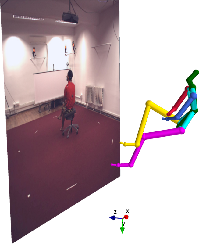
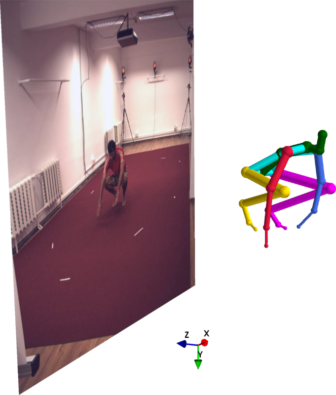
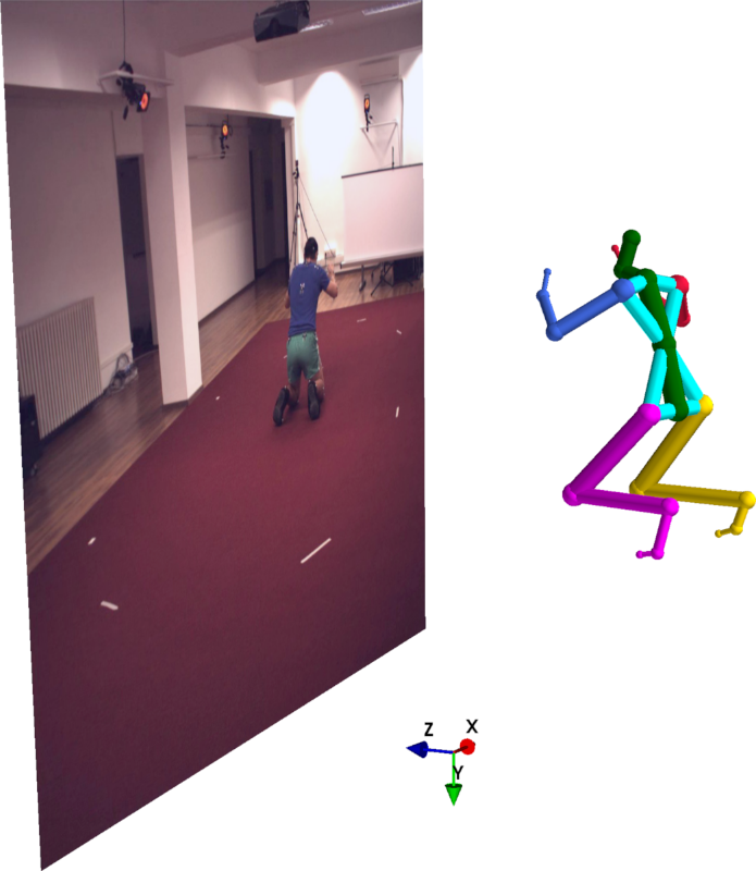
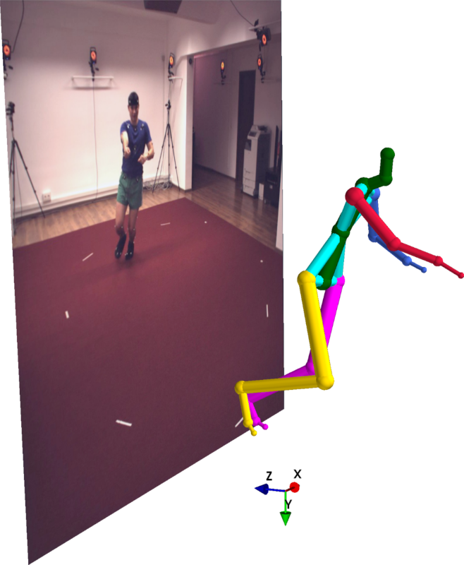
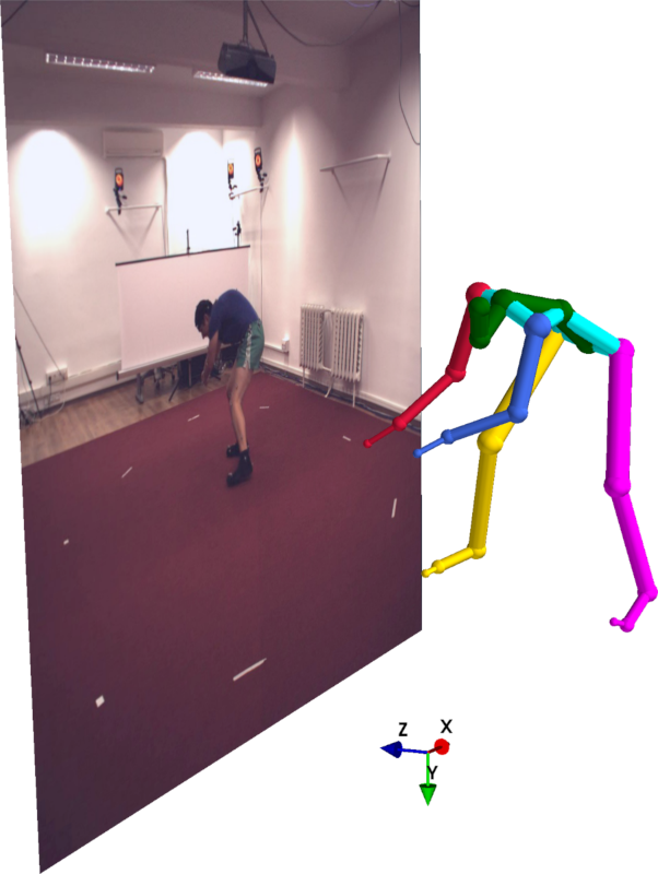
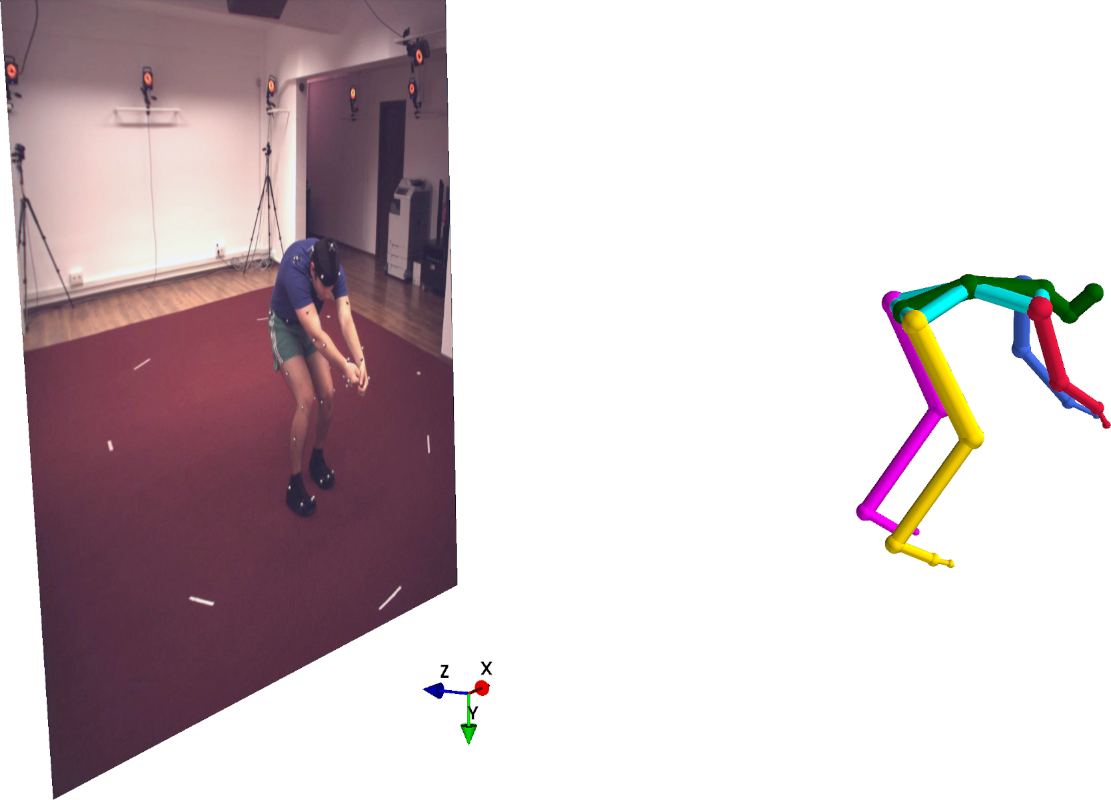
Figure 3: Absolute 3D pose predictions from monocular single images by our method.

5.5 Qualitative results

In Fig. 3 we present some qualitative results of predicted absolute 3D poses by our method. Not that the distance from predictions to the images are proportional to the absolute distance in $z$. In Fig. 7 we show monocular predictions by our method on the MPI-INF-3DHP dataset, including challenging outdoor scenes, which are not present in the training set. Finally, in Fig. 8, we show the results from our consensus-based optimization approach, from multi-view predictions on Human3.6M. Finally, in Fig. 9, we show some generalization results from our method trained on Human3.6, considering predictions on challenging images from Penn Action dataset.

5.6 Ablation studies

In this part, we present additional experiments to provide insights about our method and our design choices.

Network architecture. We evaluated three different network architectures as presented in Table 4. An off-the-shelf ResNet performed 62.2mm and 53.7mm, respectively when cut at blocks 4 and 5. The proposed ResNet-U improves on ResNet block 5 by 3.2mm while requiring 2.7M less parameters.

Table 4: Evaluation of the network architecture, considering the backbone only (ResNet) cut at block 4 and block 5, and the refinement network (ResNet-U).

ResNet block 4		ResNet block 5		ResNet-U
MPJPE	#Par.	MPJPE	#Par.	MPJPE	#Par.
62.2	10.5M	53.7	26M	50.5	23.3M

Absolute depth estimation. In Table 5, we evaluate the influence of visual features and bounding box position for the absolute depth estimation, considering the mean root position error in mm (MRPE). As can be observed, using only bounding box features is insufficient to precisely predict the absolute $\hat{\mathit{z}}_{a}{}$, but when combined with visual features it further improves by 20mm, which evidences the need of a global bounding box information for that task.

Table 5: Absolute root joint position error in mm based on different features combinations.

Features	Bounding box	CNN features	Combined
MRPE	375.4	100.1	80.1

The effect of multiple camera views. Since the proposed method predicts 3D poses in absolute camera coordinates and is also capable of estimating the extrinsic camera parameters, we can use multiple cameras to predict the same pose at inference time. When considering multi-view scenarios, we can either use camera calibration, when provided, or we can use our consensus-based optimization algorithm.

In Table 6 we present our results considering both 3D pose estimation and absolute root position errors, as well as estimated and ground truth camera parameters. We use multiple combinations of cameras, in order to show the influence of different number of views. As we can see, each camera lowers the error by about 5mm, which is significant on Human3.6M. We can also notice that our consensus optimization approach is capable of providing highly precise estimation, even under uncalibrated conditions.

Table 6: Results of our method on 3D human pose estimation and on root joint absolute error (MPJPE / MRPE) considering single and multi-view with different camera combinations.

Method	GT camera		Estimated camera
	MPJPE	MRPE	MPJPE	MRPE
Monocular	50.5	80.1	–	–
Monocular + h.flip	49.2	79.9	–	–
Cameras 1,2	45.7	73.3	52.2	167.0
Cameras 1,4	46.2	74.9	59.0	171.0
Cameras 1,2,3	41.8	57.4	47.9	143.8
Cameras 1,2,3,4	36.9	51.0	44.7	130.7

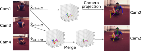
Figure 4: On top, the absolute prediction from camera 1 is projected into camera 2 with considerable errors in occluded joints. At the bottom, predictions from cameras 1, 3, 4 are projected into camera 2 and merged, improving the prediction significantly.

Zero-shot on new camera setup. We evaluated our method in a new camera setup considering a zero-shot scenario, where we used our model trained on Human3.6M and and evaluated it on KTH. Due to the high disparity in the camera intrinsics between both datasets, the absolute depth predictions stayed in the range observed in Human3.6M, with an average of $4.040$ meters. The consensus-based algorithm still converged in the multi-view scenario, even though the final 3D poses are shifted to a smaller size due to the absolute depth predicted by our method (see Fig. 5). To correct the scale and shift, we rescaled the predicted 3D poses using the torso size from KTH (the length from the neck to the hip center) and shifted our predictions to the KTH poses in the hip center. After this, we computed the PCP metrics of our predictions, which results in $0.812$ and $.929$ for lower and upper legs, and in $0.620$ and $0.804$ for lower and upper arms. Additional qualitative results on KTH are shown in Fig. 6, where the final 3D estimations are also projected to the source images.

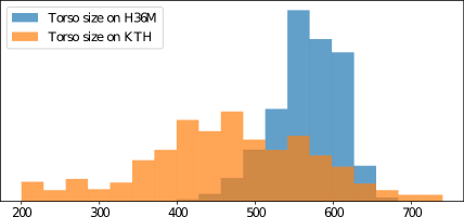
Figure 5: Torso size in mm of our estimated 3D poses on Human3.6M and on KTH, considering a zero-shot scenario.

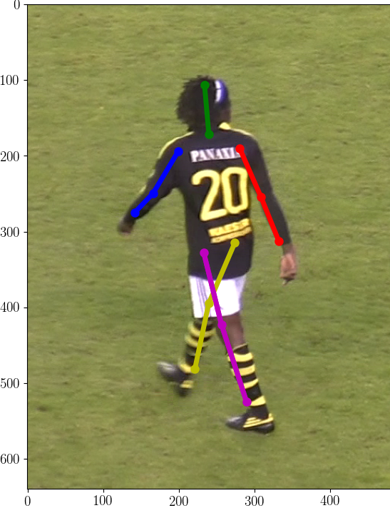
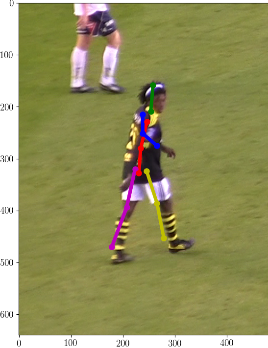
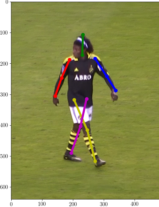
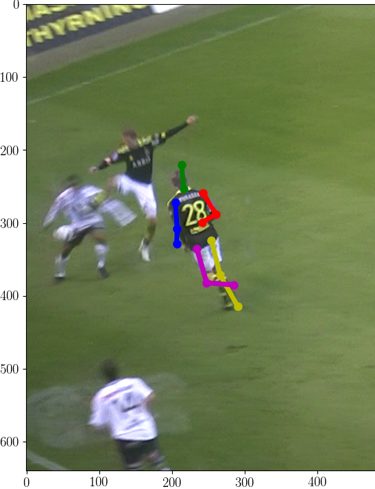
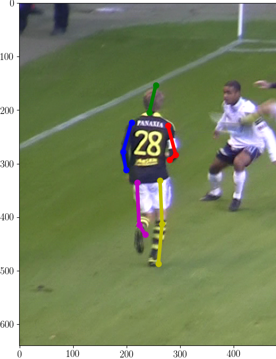
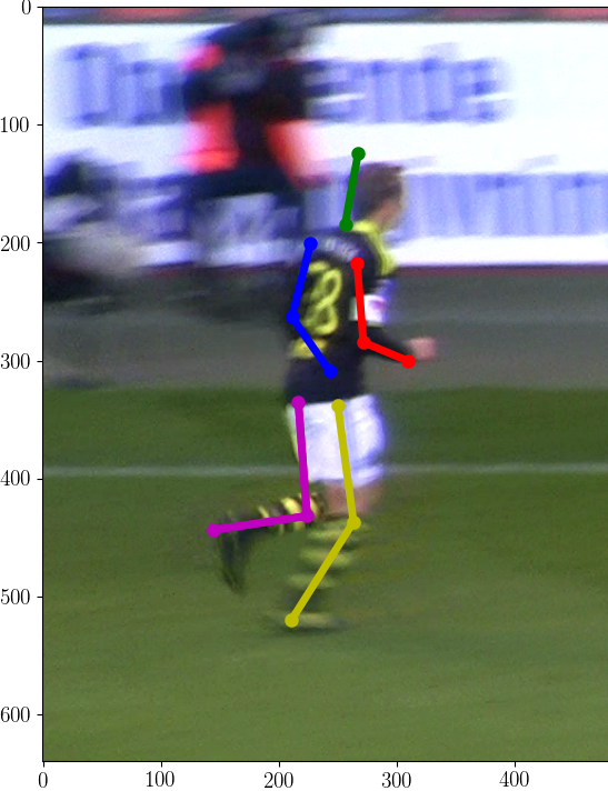
Figure 6: Qualitative results on KTH: projections of estimated 3D poses by our model trained on H36M.

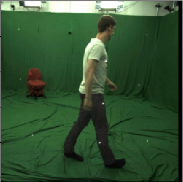
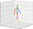
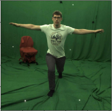
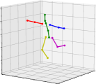
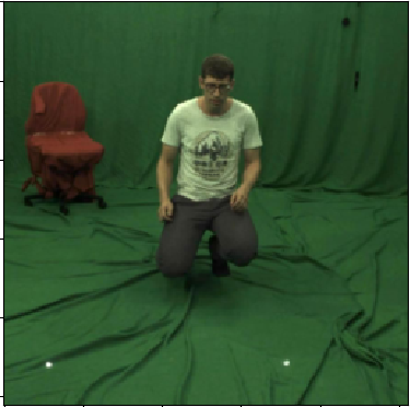
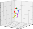
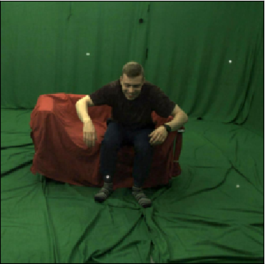
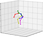
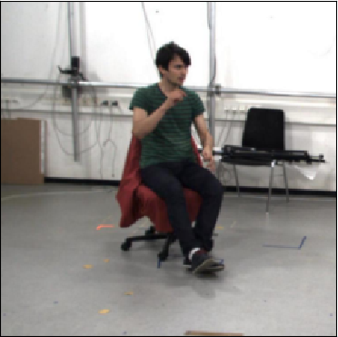
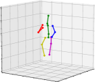
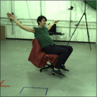
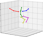
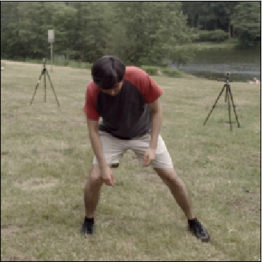
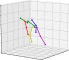
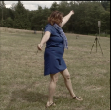
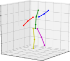
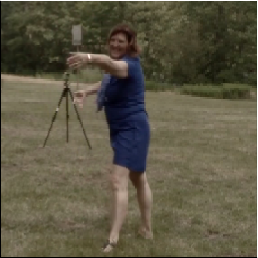
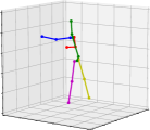
Figure 7: 3D pose predictions from monocular single images on MPI-INF-3DHP dataset, including indoor and outdoor scenes.

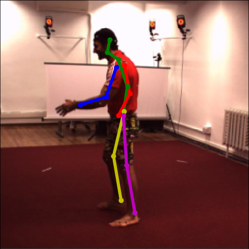
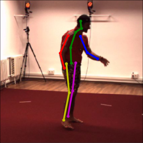
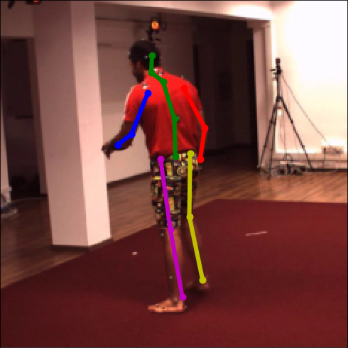
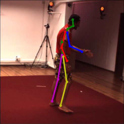
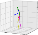
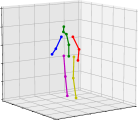
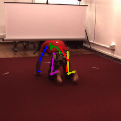
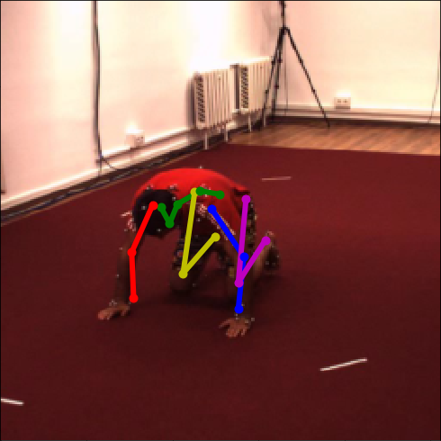
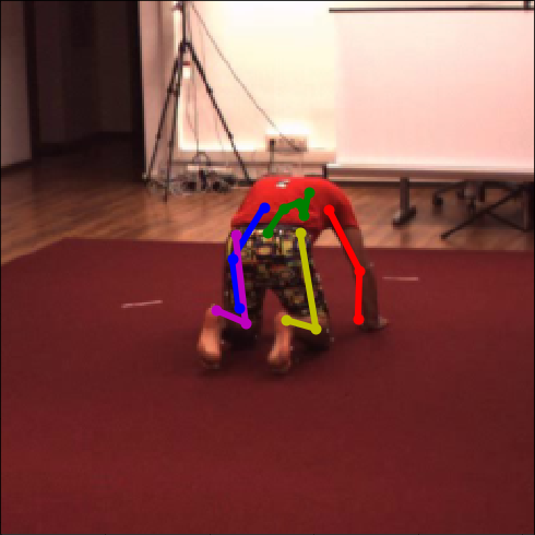
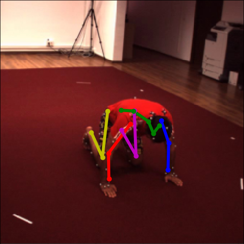
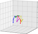
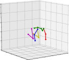
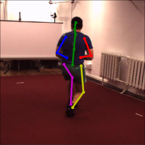
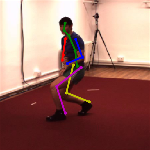
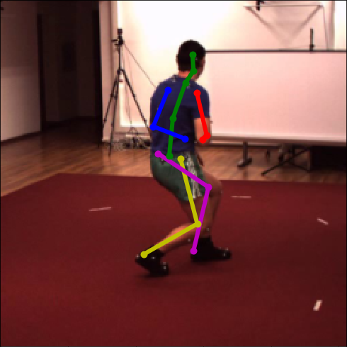
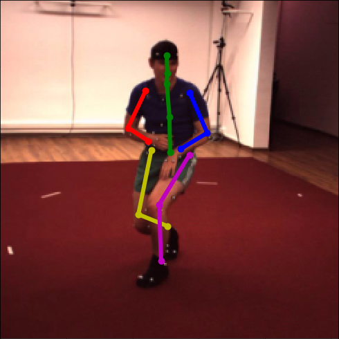
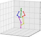
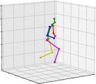
Figure 8: 3D pose predictions from our consensus-based optimization algorithm, considering multi-view on Human3.6M. Final 3D poses are projected into the different views (a,b,c,d) and shown in perspective (e,f).

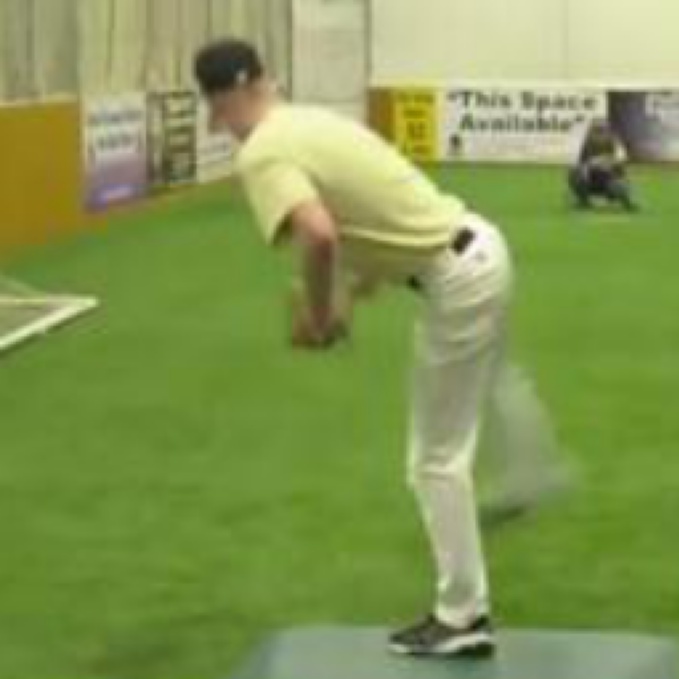
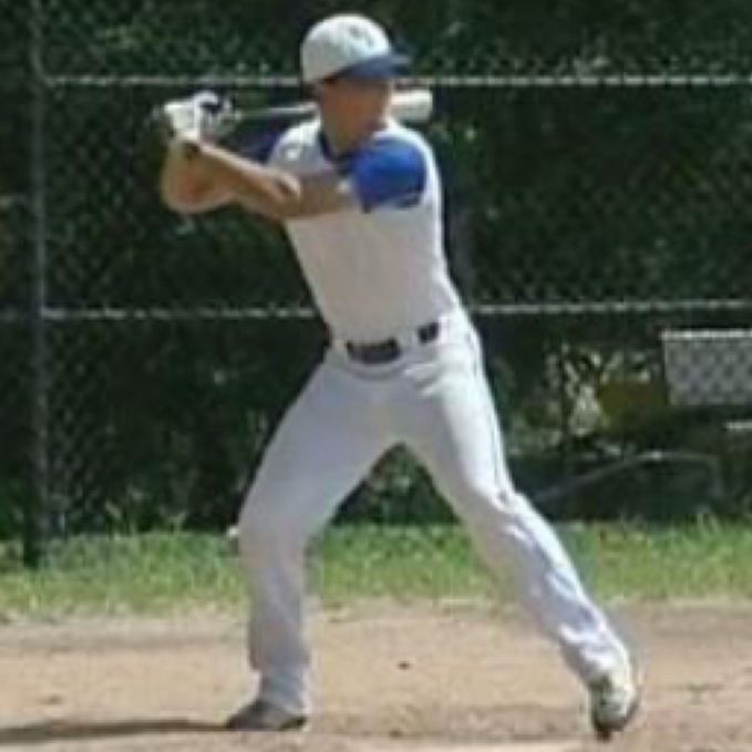
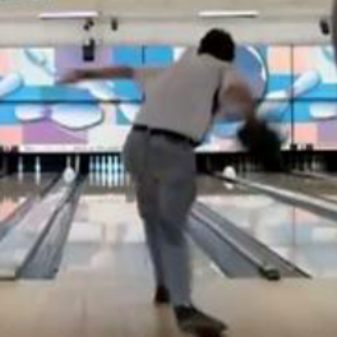
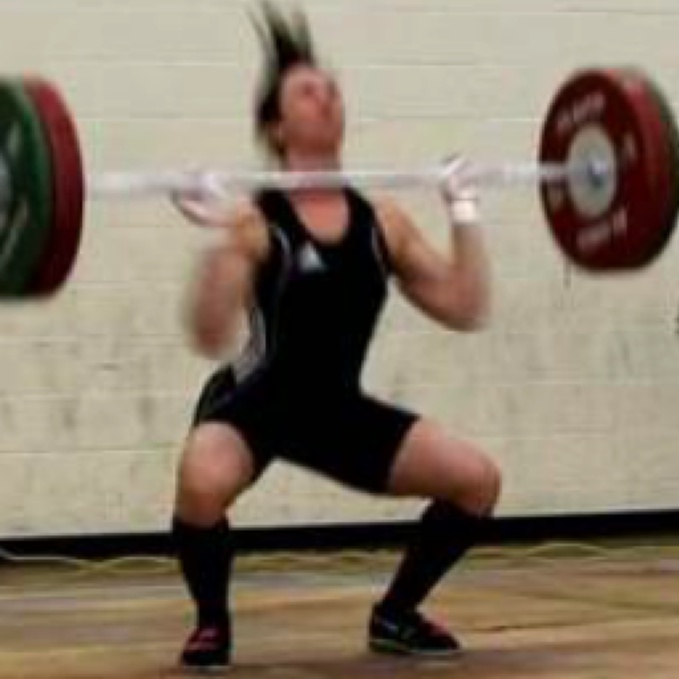
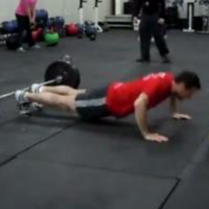
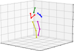
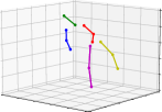
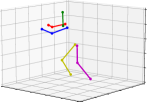
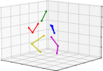
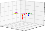
Figure 9: Generalization of our method for 3D pose estimation on unseen dataset (PennAction), including outdoor scenes in different contexts.

Finally, Fig. 4 shows an example of highly occluded body parts where multiple camera predictions results in a significantly better reconstruction. Note that in this case we are projecting the estimated absolute 3D pose to a new point of view, not used during inference. Despite the highly occluded joints in some views, the resulting absolute pose is very coherent and has a reduced shift when our consensus-based algorithm is used.

5.7 Discussion

In the proposed approach, we have the advantage of predicting 3D human poses in absolute coordinates, which enables performing multi-view estimations while training the neural network model with monocular images. This aspect allows our method to be easily adapted to a variable number of cameras, without any additional training cost, as demonstrated in Table 6. On the other hand, our method requires absolute 3D poses during training, which is a limiting factor, specially for training on datasets that provides only normalised human poses. The trained model can also be limited by the low variability of camera intrinsics during training, which may result in shift and scale deviations during inference on different cameras. As a future work, the proposed consensus-based optimization could be further integrated in the training pipeline, in order to allow a training process based on multiple views of the scene.

6 Conclusions

In this paper, we have proposed a new method for the problem of predicting 3D human poses in absolute coordinates and a new algorithm for multi-view predictions optimization. We show that, by casting the problem into a new perspective, we can benefit from training with 2D and 3D data indistinguishably, while performing 3D predictions in a more effective way. These improvements boost monocular 3D pose estimation significantly. As another consequence of the absolute prediction, we show that multi-view estimations can be easily performed from multiple absolute monocular estimations, resulting in much higher precision than previous methods in the literature, even when considering multiple uncalibrated images.

References

- [1] A. Agarwal and B. Triggs. Recovering 3D human pose from monocular images. IEEE Trans. Pattern Anal. Mach. Intell. (TPAMI), 28(1):44–58, Jan 2006.
- [2] S. Amin, M. Andriluka, M. Rohrbach, and B. Schiele. Multi-view pictorial structures for 3d human pose estimation. In The British Machine Vision Conference (BMVC), 2013.
- [3] M. Andriluka, L. Pishchulin, P. Gehler, and B. Schiele. 2D Human Pose Estimation: New Benchmark and State of the Art Analysis. In The IEEE Conference on Computer Vision and Pattern Recognition (CVPR), June 2014.
- [4] V. Belagiannis, S. Amin, M. Andriluka, B. Schiele, N. Navab, and S. Ilic. 3D pictorial structures for multiple human pose estimation. In The IEEE Conference on Computer Vision and Pattern Recognition (CVPR), pages 1669–1676, 2014.
- [5] Belagiannis, Vasileios and Amin, Sikandar and Andriluka, Mykhaylo and Schiele, Bernt and Navab, Nassir and Ilic, Slobodan. 3d pictorial structures revisited: Multiple human pose estimation. IEEE Trans. Pattern Anal. Mach. Intell. (TPAMI), 38(10):1929–1942, Oct. 2016.
- [6] M. Burenius, J. Sullivan, and S. Carlsson. 3D pictorial structures for multiple view articulated pose estimation. In The IEEE Conference on Computer Vision and Pattern Recognition (CVPR), pages 3618–3625, 2013.
- [7] M. Burenius, J. Sullivan, and S. Carlsson. 3d pictorial structures for multiple view articulated pose estimation. In 2013 IEEE Conference on Computer Vision and Pattern Recognition, pages 3618–3625, 2013.
- [8] C.-H. Chen and D. Ramanan. 3D Human Pose Estimation = 2D Pose Estimation + Matching. In The IEEE Conference on Computer Vision and Pattern Recognition (CVPR), 2017.
- [9] W. Chen, Z. Fu, D. Yang, and J. Deng. Single-Image Depth Perception in the Wild. In D. D. Lee, M. Sugiyama, U. V. Luxburg, I. Guyon, and R. Garnett, editors, Advances in Neural Information Processing Systems 29, pages 730–738. 2016.
- [10] T. v. Dijk and G. d. Croon. How Do Neural Networks See Depth in Single Images? In The IEEE International Conference on Computer Vision (ICCV), October 2019.
- [11] D. Eigen, C. Puhrsch, and R. Fergus. Depth Map Prediction from a Single Image using a Multi-Scale Deep Network. In Z. Ghahramani, M. Welling, C. Cortes, N. D. Lawrence, and K. Q. Weinberger, editors, Advances in Neural Information Processing Systems 27, pages 2366–2374. 2014.
- [12] S. Gunel, H. Rhodin, and P. Fua. What face and body shapes can tell us about height. In Proceedings of the IEEE/CVF International Conference on Computer Vision (ICCV) Workshops, Oct 2019.
- [13] K. He, X. Zhang, S. Ren, and J. Sun. Deep residual learning for image recognition. In The IEEE Conference on Computer Vision and Pattern Recognition (CVPR), pages 770–778, 2016.
- [14] M. Hofmann and D. M. Gavrila. Multi-view 3D Human Pose Estimation in Complex Environment. International Journal of Computer Vision, 96(1):103–124, Jan 2012.
- [15] C. Ionescu, F. Li, and C. Sminchisescu. Latent structured models for human pose estimation. In International Conference on Computer Vision (ICCV), pages 2220–2227, Nov 2011.
- [16] C. Ionescu, D. Papava, V. Olaru, and C. Sminchisescu. Human3.6M: Large Scale Datasets and Predictive Methods for 3D Human Sensing in Natural Environments. IEEE Trans. Pattern Anal. Mach. Intell. (TPAMI), 36(7):1325–1339, jul 2014.
- [17] K. Iskakov, E. Burkov, V. Lempitsky, and Y. Malkov. Learnable triangulation of human pose. In Proceedings of the IEEE/CVF International Conference on Computer Vision, pages 7718–7727, 2019.
- [18] A. Kadkhodamohammadi and N. Padoy. A generalizable approach for multi-view 3d human pose regression. Machine Vision and Applications, 32(1):1–14, 2021.
- [19] V. Kazemi, M. Burenius, H. Azizpour, and J. Sullivan. Multi-view body part recognition with random forests. In 2013 24th British Machine Vision Conference, BMVC 2013; Bristol; United Kingdom; 9 September 2013 through 13 September 2013. British Machine Vision Association, 2013.
- [20] Kocabas, Muhammed and Karagoz, Salih and Akbas, Emre. Self-supervised learning of 3d human pose using multi-view geometry. In The IEEE Conference on Computer Vision and Pattern Recognition (CVPR), June 2019.
- [21] N. Kolotouros, G. Pavlakos, M. J. Black, and K. Daniilidis. Learning to reconstruct 3d human pose and shape via model-fitting in the loop. In Proceedings of the IEEE/CVF International Conference on Computer Vision (ICCV), October 2019.
- [22] I. Laina, C. Rupprecht, V. Belagiannis, F. Tombari, and N. Navab. Deeper depth prediction with fully convolutional residual networks. In International Conference on 3D vision (3DV), pages 239–248. IEEE, 2016.
- [23] K. Lee, I. Lee, and S. Lee. Propagating LSTM: 3D Pose Estimation based on Joint Interdependency. In The European Conference on Computer Vision (ECCV), September 2018.
- [24] S. Li, W. Zhang, and A. B. Chan. Maximum-Margin Structured Learning With Deep Networks for 3D Human Pose Estimation. In The IEEE International Conference on Computer Vision (ICCV), December 2015.
- [25] D. C. Luvizon, D. Picard, and H. Tabia. 2D/3D Pose Estimation and Action Recognition Using Multitask Deep Learning. In The IEEE Conference on Computer Vision and Pattern Recognition (CVPR), June 2018.
- [26] D. C. Luvizon, H. Tabia, and D. Picard. Human pose regression by combining indirect part detection and contextual information. Computers & Graphics, 85:15–22, 2019.
- [27] J. Martinez, R. Hossain, J. Romero, and J. J. Little. A simple yet effective baseline for 3d human pose estimation. In ICCV, 2017.
- [28] D. Mehta, H. Rhodin, D. Casas, P. Fua, O. Sotnychenko, W. Xu, and C. Theobalt. Monocular 3D Human Pose Estimation In The Wild Using Improved CNN Supervision. In International Conference on 3D vision (3DV), 2017.
- [29] D. Mehta, O. Sotnychenko, F. Mueller, W. Xu, M. Elgharib, P. Fua, H.-P. Seidel, H. Rhodin, G. Pons-Moll, and C. Theobalt. XNect: Real-time multi-person 3D motion capture with a single RGB camera. volume 39, 2020.
- [30] D. Mehta, S. Sridhar, O. Sotnychenko, H. Rhodin, M. Shafiei, H.-P. Seidel, W. Xu, D. Casas, and C. Theobalt. Vnect: Real-time 3d human pose estimation with a single rgb camera. volume 36, 2017.
- [31] B. Micusik and T. Pajdla. Simultaneous surveillance camera calibration and foot-head homology estimation from human detections. In 2010 IEEE Computer Society Conference on Computer Vision and Pattern Recognition (CVPR), pages 1562–1569, 2010.
- [32] G. Moon, J. Y. Chang, and K. M. Lee. Camera Distance-Aware Top-Down Approach for 3D Multi-Person Pose Estimation From a Single RGB Image. In The IEEE International Conference on Computer Vision (ICCV), October 2019.
- [33] P. K. Nathan Silberman, Derek Hoiem and R. Fergus. Indoor Segmentation and Support Inference from RGBD Images. In ECCV, 2012.
- [34] A. Newell, K. Yang, and J. Deng. Stacked Hourglass Networks for Human Pose Estimation. The European Conference on Computer Vision (ECCV), pages 483–499, 2016.
- [35] B. X. Nie, P. Wei, and S.-C. Zhu. Monocular 3D human pose estimation by predicting depth on joints. In The IEEE International Conference on Computer Vision (ICCV), pages 3467–3475. IEEE, 2017.
- [36] J. C. Núñez, R. Cabido, J. F. Vélez, A. S. Montemayor, and J. J. Pantrigo. Multiview 3D human pose estimation using improved least-squares and LSTM networks. Neurocomputing, 323:335 – 343, 2019.
- [37] G. Pavlakos, X. Zhou, K. G. Derpanis, and K. Daniilidis. Coarse-to-Fine Volumetric Prediction for Single-Image 3D Human Pose. In The IEEE Conference on Computer Vision and Pattern Recognition (CVPR), 2017.
- [38] G. Pavlakos, X. Zhou, K. G. Derpanis, and K. Daniilidis. Harvesting Multiple Views for Marker-less 3D Human Pose Annotations. In The IEEE Conference on Computer Vision and Pattern Recognition (CVPR), 2017.
- [39] A. Popa, M. Zanfir, and C. Sminchisescu. Deep Multitask Architecture for Integrated 2D and 3D Human Sensing. In The IEEE Conference on Computer Vision and Pattern Recognition (CVPR), pages 4714–4723, 2017.
- [40] M. Rayat Imtiaz Hossain and J. J. Little. Exploiting temporal information for 3D human pose estimation. In The European Conference on Computer Vision (ECCV), September 2018.
- [41] J. Redmon and A. Farhadi. YOLO9000: Better, Faster, Stronger. In The IEEE Conference on Computer Vision and Pattern Recognition (CVPR), 2017.
- [42] H. Rhodin, J. Spörri, I. Katircioglu, V. Constantin, F. Meyer, E. Müller, M. Salzmann, and P. Fua. Learning monocular 3d human pose estimation from multi-view images. In The IEEE Conference on Computer Vision and Pattern Recognition (CVPR), pages 8437–8446, 2018.
- [43] G. Rogez, P. Weinzaepfel, and C. Schmid. LCR-Net: Localization-Classification-Regression for Human Pose. In The IEEE Conference on Computer Vision and Pattern Recognition (CVPR), June 2017.
- [44] N. Sarafianos, B. Boteanu, B. Ionescu, and I. A. Kakadiaris. 3D Human pose estimation: A review of the literature and analysis of covariates. Computer Vision and Image Understanding, 152:1–20, 2016.
- [45] Y. Shi, X. Han, N. Jiang, K. Zhou, K. Jia, and J. Lu. Fbi-pose: Towards bridging the gap between 2d images and 3d human poses using forward-or-backward information. CoRR, 2018.
- [46] X. Sun, J. Shang, S. Liang, and Y. Wei. Compositional Human Pose Regression. In The IEEE International Conference on Computer Vision (ICCV), Oct 2017.
- [47] X. Sun, B. Xiao, F. Wei, S. Liang, and Y. Wei. Integral Human Pose Regression. In The European Conference on Computer Vision (ECCV), September 2018.
- [48] B. Tekin, I. Katircioglu, M. Salzmann, V. Lepetit, and P. Fua. Structured Prediction of 3D Human Pose with Deep Neural Networks. In The British Machine Vision Conference (BMVC), 2016.
- [49] D. Tome, C. Russell, and L. Agapito. Lifting From the Deep: Convolutional 3D Pose Estimation From a Single Image. In The IEEE Conference on Computer Vision and Pattern Recognition (CVPR), 2017.
- [50] D. Tome, M. Toso, L. Agapito, and C. Russell. Rethinking pose in 3d: Multi-stage refinement and recovery for markerless motion capture. In 2018 international conference on 3D vision (3DV), pages 474–483. IEEE, 2018.
- [51] M. Trumble, A. Gilbert, A. Hilton, and J. Collomosse. Deep autoencoder for combined human pose estimation and body model upscaling. In The European Conference on Computer Vision (ECCV), pages 784–800, 2018.
- [52] M. Trumble, A. Gilbert, C. Malleson, A. Hilton, and J. Collomosse. Total Capture: 3D Human Pose Estimation Fusing Video and Inertial Sensors. In The British Machine Vision Conference (BMVC), 2017.
- [53] I. Vasiljevic, N. Kolkin, S. Zhang, R. Luo, H. Wang, F. Z. Dai, A. F. Daniele, M. Mostajabi, S. Basart, M. R. Walter, and G. Shakhnarovich. DIODE: A Dense Indoor and Outdoor DEpth Dataset. CoRR, abs/1908.00463, 2019.
- [54] W. Yang, W. Ouyang, X. Wang, J. Ren, H. Li, and X. Wang. 3D Human Pose Estimation in the Wild by Adversarial Learning. In The IEEE Conference on Computer Vision and Pattern Recognition (CVPR), June 2018.
- [55] K. M. Yi, E. Trulls, V. Lepetit, and P. Fua. LIFT: Learned Invariant Feature Transform. The European Conference on Computer Vision (ECCV), 2016.
- [56] A. Zanfir, E. Marinoiu, and C. Sminchisescu. Monocular 3D Pose and Shape Estimation of Multiple People in Natural Scenes - The Importance of Multiple Scene Constraints. In The IEEE Conference on Computer Vision and Pattern Recognition (CVPR), June 2018.
- [57] A. Zanfir, E. Marinoiu, M. Zanfir, A.-I. Popa, and C. Sminchisescu. Deep Network for the Integrated 3D Sensing of Multiple People in Natural Images. In S. Bengio, H. Wallach, H. Larochelle, K. Grauman, N. Cesa-Bianchi, and R. Garnett, editors, Advances in Neural Information Processing Systems 31, pages 8410–8419. 2018.
- [58] W. Zhang, M. Zhu, and K. G. Derpanis. From actemes to action: A strongly-supervised representation for detailed action understanding. In 2013 IEEE International Conference on Computer Vision, pages 2248–2255, 2013.
- [59] X. Zhou, Q. Huang, X. Sun, X. Xue, and Y. Wei. Towards 3D Human Pose Estimation in the Wild: A Weakly-Supervised Approach. In The IEEE International Conference on Computer Vision (ICCV), Oct 2017.
- [60] X. Zhou, X. Sun, W. Zhang, S. Liang, and Y. Wei. Deep Kinematic Pose Regression. Computer Vision ECCV 2016 Workshops, 2016.
- [61] X. Zhou, M. Zhu, S. Leonardos, K. G. Derpanis, and K. Daniilidis. Sparseness Meets Deepness: 3D Human Pose Estimation From Monocular Video. In The IEEE Conference on Computer Vision and Pattern Recognition (CVPR), June 2016.
- [62] H. Zou and T. Hastie. Regularization and variable selection via the Elastic Net. Journal of the Royal Statistical Society, Series B, 67:301–320, 2005.