The Karger-Stein Algorithm is Optimal for $k$-cut

Abstract

In the $k$-cut problem, we are given an edge-weighted graph and want to find the least-weight set of edges whose deletion breaks the graph into $k$ connected components. Algorithms due to Karger-Stein and Thorup showed how to find such a minimum $k$-cut in time approximately $O(n^{2k-2})$. The best lower bounds come from conjectures about the solvability of the $k$-clique problem and a reduction from $k$-clique to $k$-cut, and show that solving $k$-cut is likely to require time $\Omega(n^{k})$. Our recent results have given special-purpose algorithms that solve the problem in time $n^{1.98k+O(1)}$, and ones that have better performance for special classes of graphs (e.g., for small integer weights).

In this work, we resolve the problem for general graphs, by showing that for any fixed $k\geq 2$, the Karger-Stein algorithm outputs any fixed minimum $k$-cut with probability at least $\widehat{O}(n^{-k})$, where $\widehat{O}(\cdot)$ hides a $2^{O(\ln\ln n)^{2}}$ factor. This also gives an extremal bound of $\widehat{O}(n^{k})$ on the number of minimum $k$-cuts in an $n$-vertex graph and an algorithm to compute a minimum $k$-cut in similar runtime. Both are tight up to $\widehat{O}(1)$ factors.

The first main ingredient in our result is a fine-grained analysis of how the graph shrinks—and how the average degree evolves—under the Karger-Stein process. The second ingredient is an extremal result bounding the number of cuts of size at most $(2-\delta)OPT/k$, using the Sunflower lemma.

1 Introduction

We consider the $k\textsc{-Cut}$ problem: given an edge-weighted graph $G=(V,E,w)$ and an integer $k$, delete a minimum-weight set of edges so that $G$ has at least $k$ connected components. This problem generalizes the global min-cut problem, where the goal is to break the graph into $k=2$ pieces. It was unclear that the problem admitted a polynomial-time algorithm for fixed values of $k$, until the work of Goldschmidt and Hochbaum, who gave a runtime of $O(n^{(1/2-o(1))k^{2}})$ [GH94]. (Here and subsequently, the $o(1)$ in the exponent indicates a quantity that goes to $0$ as $k$ increases.) The randomized minimum-cut algorithm of Karger and Stein [KS96], based on random edge contractions, can be used to solve $k\textsc{-Cut}$ in $\tilde{O}(n^{2(k-1)})$ time. For deterministic algorithms, there have been improvements to the Goldschmidt and Hochbaum result [KYN07, Tho08, CQX18]: notably, the tree-packing result of Thorup [Tho08] was sped up by Chekuri et al. [CQX18] to run in $O(mn^{2k-3})$ time. Hence, until recently, randomized and deterministic algorithms using very different approaches achieved $O(n^{(2-o(1))k})$ bounds for the problem.

On the hardness side, one can reduce Max-Weight $(k-1)$-Clique to $k\textsc{-Cut}$. It is conjectured that solving Max-Weight $(k-1)$-Clique requires $\tilde{\Omega}(n^{(1-o(1))k})$ time when weights are integers in the range $[1,\Omega(n^{k})]$, and $\tilde{\Omega}(n^{(\omega/3)k})$ time for unit weights; here $\omega$ is the matrix multiplication constant. Hence, these runtime lower bounds also extend to the $k\textsc{-Cut}$, suggesting that $\Omega(n^{k})$ may be the optimal runtime for general weighted $k$-cut instances.

There has been recent progress on this problem, showing the following results:

1. We showed an $O(n^{(1.98+o(1))k})$-time algorithm for general $k\textsc{-Cut}$ [GLL19]. This was based on giving an extremal bound on the maximum number of “small” cuts in the graph, and then using a bounded-depth search approach to guess the small cuts within the optimal $k$-cut and make progress. This was a proof-of-concept result, showing that the bound of $n^{(2-o(1))k}$ was not the right bound, but it does not seem feasible to improve that approach to exponents considerably below $2k$.

2. For graphs with polynomial integer weights, we showed how to solve the problem in time approximately $k^{O(k)}\,n^{(2\omega/3+o(1))k}$ [GLL18]. And for unweighted graphs we showed how to get the $k^{O(k)}n^{(1+o(1)k}$ runtime [Li19]. Both these approaches were based on obtaining a spanning tree cut by a minimum $k$-cut in a small number of edges, and using involved dynamic programming methods on the tree to efficiently compute the edges and find the $k$-cut. The former relied on matrix multiplication ideas, and the latter on the Kawarabayashi-Thorup graph decomposition, both of which are intrinsically tied to graphs with small edge-weights.

In this paper, we show that the “right” algorithm, the original Karger-Stein algorithm, achieves the “right” bound for general graphs. Our main result is the following.

Theorem 1 (Main).

Given a graph $G$ and a parameter $k\geq 2$, the Karger-Stein algorithm outputs any fixed minimum $k$-cut in $G$ with probability at least $n^{-k}\cdot(k\ln n)^{-O(k^{2}\ln\ln n)}$.

For any fixed constant $k\geq 2$, the above bound becomes $n^{k}\cdot 2^{O(\ln\ln n)^{2}}$. This immediately implies the following two corollaries, where $\widehat{O}(\cdot)$ hides a quasi-logarithmic factor $2^{O(\ln\ln n)^{2}}$:

Corollary 2 (Number of Minimum $k$-cuts).

For any fixed $k\geq 2$, the number of minimum-weight $k$-cuts in a graph is at most $\widehat{O}(n^{k})$.

This bound significantly improves the previous best bound $n^{(1.98+o(1))k}$ [GLL19]. It is also almost tight because the cycle on $n$ vertices has $\Omega(n^{k})$ minimum $k$-cuts.

Corollary 3 (Faster Algorithm to Find a Minimum $k$-cut).

For any fixed $k\geq 2$, there is a randomized algorithm that computes a minimum $k$-cut of a graph with high probability in time $\widehat{O}(n^{k})$.

This improves the running time $n^{(1.98+o(1))k}$ for the general weighted case [GLL19] and even the running time $n^{(1+o(1))k}$ for the unweighted case [Li19], where the extra $n^{o(k)}$ term is still at least polynomial for fixed $k$. It is also almost tight under the hypothesis that Max-Weight $(k-1)$-Clique requires $\tilde{\Omega}(n^{(1-o(1))k})$ time.

1.1 Our Techniques

Let us first recall the Karger-Stein algorithm:

Algorithm 1 Karger-Stein Algorithm

1:procedure Karger-Stein($G=(V,E,w)$, $k\in\mathbb{N}$) $\triangleright$ Compute a minimum $k$-cut of $G$

2:     while $|V|>k$ do

3:         Sample an edge $e\in E$ with probability proportional to $w(e)$.

4:         Contract two vertices in $e$ and remove self-loops. $\triangleright$ $|V|$ decreases by exactly $1$

5:     end while

6:     Return the $k$-cut of the original graph by expanding the vertices of $V$.

7:end procedure

In the spirit of [GLL19], our proof consists of two main parts: (i) a new algorithmic analysis (this time for the Karger-Stein algorithm), and (ii) a statement on the extremal number of “small” cuts in a graph. In order to motivate the new analysis of Karger-Stein, let us first state a crude version of our extremal result. Define $\lambda_{k}$ as the minimum $k$-cut value of the graph. Think of $\overline{\lambda}_{k}:=\lambda_{k}/k$ as the average contribution of each of the $k$ components to the $k$-cut. Loosely speaking, the extremal bound says the following:

$(\star)$ There are a linear number of cuts of a graph of size at most $1.99\overline{\lambda}_{k}$.

To develop some intuition for this claim, we make two observations about the cycle and clique graphs, two graphs where the number of minimum $k$-cuts is indeed $\Omega(n^{k})$. Firstly, in the $n$-cycle, $\overline{\lambda}_{k}=1=\lambda/2$ for any value of $k$, and since $1.99\overline{\lambda}_{k}=1.99<2=\lambda$, so there are no cuts in the graph with size at most $1.99\overline{\lambda}_{k}$, hence $(\star)$ holds. However, it breaks if $1.99\overline{\lambda}_{k}$ is replaced by $2\overline{\lambda}_{k}$, since there are $\binom{n}{2}$ many cuts of size $2\overline{\lambda}_{k}=2=\lambda$. Secondly, for the $n$-clique we have $\lambda_{k}\approx k(n-1)$, since the minimum $k$-cut chops off $k-1$ singleton vertices. (We assume $k\ll n$, and ignore the $\binom{k}{2}$ double-counted edges for simplicity.) We have $\overline{\lambda}_{k}\approx n-1=\lambda$ instead for the $n$-clique, and there are exactly $n$ cuts of size at most $1.99\overline{\lambda}_{k}$ (the singletons), so our bound $(\star)$ holds. And again, $(\star)$ fails when $1.99\overline{\lambda}_{k}$ replaced by $2$. Therefore, in both the cycle and the clique, the bound $1.99\overline{\lambda}_{k}$ is almost the best possible. Moreover, the linear bound in the number of cuts is also optimal in the clique. In general, it is instructive to consider the cycle and clique as two opposite ends of the spectrum in the context of graph cuts, since one graph has $n$ minimum cuts and the other has $\binom{n}{2}$.

1.1.1 Algorithmic Analysis.

To analyze Karger-Stein, we adopt an exponential clock view of the process: fix an infinitesimally small parameter $\delta$, and on each timestep of length $\delta$, sample each edge with an independent probability $\delta/\overline{\lambda}_{k}$ and contract it. If $\delta$ is small enough, then we can disregard the event that more than one edge is sampled on a single timestep. This perspective has a distinct advantage over the classical random contraction procedure that contracts one edge at a time: we can analyze whether each edge is contracted independently. At the same time, we reemphasize it is just another view of the same process; conditioned on the number of vertices $n^{\prime}$ in the remaining graph, the outcome of the exponential clock procedure has exactly the same distribution as the standard Karger-Stein procedure that iteratively contracted $n-n^{\prime}$ edges.

Let us first translate the classical Karger-Stein analysis in the exponential clock setting. Suppose that we run the process for $2\ln n$ units of time (that is, $\frac{2\ln n}{\delta}$ timesteps of length $\delta$ each). The probability that a fixed minimum $k$-cut remains at the end (i.e., has no edge contracted) is roughly

$$\left(1-\lambda_{k}\cdot\frac{\delta}{\overline{\lambda}_{k}}\right)^{(2\ln n)/\delta}\approx\exp\left(-\lambda_{k}\cdot\frac{\delta}{\overline{\lambda}_{k}}\cdot\frac{2\ln n}{\delta}\right)=\exp(2k\ln n)=n^{-2k}.$$

How many vertices are there remaining after $2\ln n$ units of time? On each $\delta$-timestep, consider the graph before any edges are contracted on this timestep. If there are currently $r\geq k-1$ vertices, then the sum of the degrees of the vertices must be at least $r\overline{\lambda}_{k}$; otherwise, we can cut out $k-1$ random singletons to obtain a $k$-cut of size at most $(k-1)\cdot\overline{\lambda}_{k}<\lambda_{k}$ (which corresponds to a $k$-cut of the same size in the original graph once we “uncontract” each edge), contradicting the definition of $\lambda_{k}$ as the minimum $k$-cut. Therefore, the graph has at least $r\overline{\lambda}_{k}/2$ edges, which means that we contract at least $r\overline{\lambda}_{k}/2\cdot\delta/\overline{\lambda}_{k}=r\delta/2$ edges in expectation. We now claim that as $\delta\to 0$, this is essentially equivalent to contracting at least $r\delta/2$ vertices in expectation, since we should not contract more than one edge at any timestep. That is, we contract a $\delta/2$ fraction of the vertices per timestep, in expectation. Therefore, after $2\ln n$ units of time (which is $\frac{2\ln n}{\delta}$ timesteps), assuming that there are always at least $k-1$ vertices remaining, the expected number of vertices remaining is at most

$$n\cdot\left(1-\frac{\delta}{2}\right)^{(2\ln n)/\delta}\approx n\cdot\exp\left(-\frac{\delta}{2}\cdot\frac{2\ln n}{\delta}\right)=n\cdot\frac{1}{n}=1.$$

Informally, we should expect to be done at around time $2\ln n$. This argument is not rigorous, since we cannot take a naïve union bound over the two successful events (namely, that no edge in the fixed $k$-cut is contracted, and there are $k-1$ vertices remaining at the end). We elaborate on how to handle this issue later on.

At any given step of the Karger-Stein process, the bound of $r\overline{\lambda}_{k}/2$ edges can be tight in the worse case. So instead of improving the analysis in a worst-case scenario, the main insight to our improvement is a more average-case improvement. At a high level, as the process continues, we expect more and more vertices in the contracted graph to have degree much higher than $\overline{\lambda}_{k}$. In fact, we show that the fraction of vertices with degree at most $1.99\overline{\lambda}_{k}$ is expected to shrink significantly throughout the process. Consequently, the total sum of degrees becomes much larger than $r\overline{\lambda}_{k}$, from which we obtain an improvement.

How do we obtain such a guarantee? Observe that every vertex of degree at most $1.99\overline{\lambda}_{k}$ in the graph at some intermediate stage of the process corresponds to a ($2$-)cut in the original graph of size at most $1.99\overline{\lambda}_{k}$. Recall that by our extremal bound, we start off with only $O_{k}(n)$ many such cuts. Some of these cuts can have size less than $\overline{\lambda}_{k}$, but we show that there cannot be too many: at most $2^{k-1}$ of them. The more interesting case is cuts of size in the range $[\overline{\lambda}_{k},1.99\overline{\lambda}_{k}]$: since each of these cuts has size at least $\overline{\lambda}_{k}$, the probability that we contract an edge in a fixed cut is at least $\overline{\lambda}_{k}\cdot\delta/\overline{\lambda}_{k}=\delta$. This means that after just $\ln n$ units of time (and not $2\ln n$), the cut remains intact only with probability $(1-\delta)^{(\ln n)/\delta}\approx 1/n$. Taking an expectation over all $O_{k}(n)$ cuts, we expect only $O_{k}(1)$ of them to remain after $\ln n$ time, which means we expect only $O_{k}(1)$ many vertices of degree at most $1.99\overline{\lambda}_{k}$ in the contracted graph after $\ln n$ time has passed. This analysis works for any time $t$: we expect only $O_{k}(n)\cdot(1-\delta)^{t/\delta}$ vertices of degree at most $1.99\overline{\lambda}_{k}$ in the contracted graph after time $t$.

This upper bound on the number of small-degree vertices lower bounds the number of edges in the graph, which in turn governs the rate at which the graph shrinks throughout the process. To obtain the optimal bounds, we model the expected rate of decrease as a differential equation. In expectation, we find that by time $\ln n$ (not $2\ln n$), we expect only $\widehat{O}_{k}(1)$ vertices remaining. This is perfect, since a fixed minimum $k$-cut survives with probability $n^{-k}$ by this time! To finish off the analysis from $\widehat{O}_{k}(1)$ vertices down to $(k-1)$ vertices, we use the regular Karger-Stein analysis, picking up an extra factor of $\left(\widehat{O}_{k}(1)\right)^{k}=\widehat{O}_{k}(1)$.

Lastly, the issue of the $\widehat{O}_{k}(1)$ vertices bound holding only in expectation requires some technical work to handle. In essence, we strengthen the expectation statement to one with high probability. We then union-bound over the event of $\widehat{O}_{k}(1)$ vertices remaining and the event that the minimum $k$-cut survives—which only holds with probability $n^{-k}$. This requires us to use concentration bounds combined with a recursive approach; the details appear in §2.2 and §2.3.

1.1.2 Extremal Result.

Recall our target extremal statement $(\star)$: there are $O_{k}(n)$ many cuts of a graph of size at most $1.99\overline{\lambda}_{k}$. Suppose for contradiction that there are $\omega_{k}(n)$ such cuts, and assume for simplicity that $k$ is even. Our goal is to select $k/2$ of these cuts that “cross in many ways”: namely, there are at least $k$ nonempty regions in their Venn diagram (see Figure 1 left). This gives a $k$-cut with total cost $k/2\cdot 1.99\overline{\lambda}_{k}<\lambda_{k}$, contradicting the definition of $\lambda_{k}$ as the minimum $k$-cut.

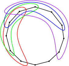
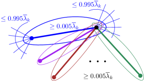
Figure 1: Left: For a contradiction, suppose all $\binom{n}{2}$ cuts of the cycle have size at most $1.99\overline{\lambda}_{k}$. Then, we select $k/2=4$ many such cuts as shown. Their Venn diagram has $8$ nonempty atoms and form an $8$-cut with cost $4\cdot 1.99\overline{\lambda}_{k}=7.92\overline{\lambda}_{k}<8\overline{\lambda}_{k}=\lambda_{k}$, contradicting the definition of $\lambda_{k}$ as the minimum $k$-cut.  Right: A $401$-sunflower with nonempty core, with the core and all petals contracted to single vertices, each of degree at least $\overline{\lambda}_{k}$. Each bolded edge must have total weight at least $0.005\overline{\lambda}_{k}$ for the corresponding cut to have size at most $1.99\overline{\lambda}_{k}$. However, the $400$ many bolded edges excluding the blue one give total weight at least $400\cdot 0.005\overline{\lambda}_{k}=2\overline{\lambda}_{k}$, and each of them crosses the blue cut, contradicting the assumption that the blue cut has size at most $1.99\overline{\lambda}_{k}$.

To find such a collection of crossing cuts, one approach is to treat each cut as a subset of vertices (the vertices on one side of the cut), and tackle the problem from a purely extremal set-theory perspective, ignoring the underlying structure of the graph. The statement becomes: given a family of $\omega_{k}(n)$ many distinct subsets of $[n]$, there exist some $k/2$ subsets whose Venn diagram has at least $k$ nonempty atoms. In [GLL19], we tackled a similar problem from this point of view. However, for our present problem, the corresponding extremal set theory statement is too good to be true. The set system $([n],\binom{[n]}{2})$ has $\binom{n}{2}$ sets, but no $k/2=3$ sets can possibly form $k=6$ regions. Hence, we need the additional structure of cuts in a graph to formulate an extremal set theoretic statement that holds.

Our key observation is that the cut structure of the graph forbids large sunflowers with nonempty core in the corresponding set family. To see why, consider a $401$-sunflower of sets $S_{1},S_{2},\ldots,S_{401}$ with nonempty core $C$, and suppose in addition that the core $C$ and each petal $S_{i}\setminus C$ is a cut of size at least $\overline{\lambda}_{k}$. (Handling cuts of size less than $\overline{\lambda}_{k}$ is a technical detail, so we omit it here.) For simplicity, consider contracting the core $C$ and petals $S_{i}\setminus C$ into single vertices $c$ and $p_{i}$, respectively. For each $i\in[401]$, the vertices $c$ and $p_{i}$ each have degree at least $\overline{\lambda}_{k}$, and yet the cut $\{c,p_{i}\}$ has size at most $1.99\overline{\lambda}_{k}$; a simple calculation shows that there must be at least $0.005\overline{\lambda}_{k}$ edges between $c$ and $p_{i}$. Equivalently, in the weighted case, the edge $(c,p_{i})$ has weight at least $0.005\overline{\lambda}_{k}$ (see Figure 1 right). Now observe that the edges $(c,p_{2}),(c,p_{3}),\ldots,(c,p_{401})$ all cross the cut $\{c,p_{1}\}$, and together, they have total weight $400\cdot 0.005\overline{\lambda}_{k}=\overline{\lambda}_{k}$. Hence, the cut $\{c,p_{1}\}$ must have weight at least $2\overline{\lambda}_{k}$, contradicting the assumption that it has size at most $1.99\overline{\lambda}_{k}$.

With this insight in mind, our modified extremal set theory statement is as follows (when $k$ is even): given a family of $\omega_{k}(n)$ many distinct subsets of $[n]$ that do not contain a $401$-sunflower with nonempty core, there exist some $k/2$ many subsets whose Venn diagram has at least $k$ nonempty atoms. This statement turns out to be true, and we provide a clean inductive argument that uses the Sunflower Lemma as a base case. (Our actual extremal statement is slightly different to handle the cuts of size less than $\overline{\lambda}_{k}$ as well as odd $k$.)

1.2 Preliminaries

A weighted graph is denoted by $G=(V,E,w)$ where $w:E\to\mathbb{Q}^{+}$ gives positive rational weights on edges. Let $\lambda_{k}$ be the weight of a minimum $k$-cut, and $\overline{\lambda}_{k}:=\lambda_{k}/k$. We use different logarithms to naturally present different parts of our analysis. We use $\ln$ to denote $\log_{e}$ and $\lg$ to denote $\log_{2}$.

2 Random Graph Process

In this section, we analyze the exponential clock viewpoint of the Karger-Stein algorithm to prove our main result Theorem 1, assuming the bound on the number of small cuts (Theorem 10) proved in Section 3.

For the sake of exposition, throughout this section, we assume $G$ is an unweighted multigraph, where the number of edges between a pair $(u,v)$ is proportional to its weight. Note that while it changes the number of edges $m$ and $\overline{\lambda}_{k}$, the resulting exponential clock procedure is still exactly equivalent to the standard Karger-Stein procedure in the original weighted graph, and the final bounds in the main lemmas (Lemma 4 and Lemma 6) only involve $n,k,t$.

2.1 Expectation

In this section, we bound the number of vertices (in expectation) at some point in the random contraction process:

Lemma 4.

Suppose $G$ has at most $\beta n$ many cuts with weight in the range $[\overline{\lambda}_{k},\gamma\overline{\lambda}_{k})$ for some constant $1\leq\gamma<2$. Fix a parameter $t\geq 0$, and suppose we contract every edge in $G$ with independent probability $1-e^{-t/\overline{\lambda}_{k}}$. Then, the expected number of vertices in the contracted graph is at most $O(\frac{\beta+1}{2-\gamma})ne^{-(\gamma/2)t}+\frac{\gamma}{2}(k-1)t$.

Consider the following exponential clock process: let each edge $e$ of the graph independently sample a random variable $x(e)$ from an exponential distribution with mean $\overline{\lambda}_{k}$, which has c.d.f.  $1-e^{-t/\overline{\lambda}_{k}}$ at value $t$. We say that the edge is sampled at time $x(e)$. Observe that for any $t\geq 0$, every edge is sampled by time $t$ with probability exactly $1-e^{-t/\overline{\lambda}_{k}}$, so this process models exactly the one in the lemma.

For a given $t\geq 0$ and $\delta>0$, the probability that an edge $e$ is sampled before time $t+\delta$, given that it is sampled after time $t$, is

$$\frac{\Pr[t\leq x(e)\leq t+\delta]}{\Pr[t\leq x(e)]}=\Pr[x(e)\leq\delta]=1-e^{-\delta/\overline{\lambda}_{k}}=\frac{\delta}{\overline{\lambda}_{k}}-O_{\overline{\lambda}_{k}}(\delta^{2}),$$

where the first equality uses the memoryless property of exponential random variables, and the $O_{\overline{\lambda}_{k}}(\cdot)$ hides the dependence on $\overline{\lambda}_{k}$. Therefore, at the loss of the $O_{\overline{\lambda}_{k}}(\delta^{2})$ factor (which we will later show to be negligible), we can imagine the “discretized” process at a small timestep $\delta$: the times $t$ are now integer multiples of $\delta$, and each edge $e$ is sampled at the (discrete) time $t$ if $t\leq e<t+\delta$. Again, the probability that an edge is sampled at (discrete) time $t+\delta$, given that it is sampled after time $t$, is $\delta/\overline{\lambda}_{k}+O_{\overline{\lambda}_{k}}(\delta^{2})\approx\delta/\overline{\lambda}_{k}$. For technical purposes, we will not assume that $t$ is always a multiple of $\delta$ in our formal argument.

Consider the graph at a given (discrete) time $t$, where we have contracted all edges sampled before time $t$ (but not those sampled at time $t$). Suppose that there are $r=r(t)$ vertices in the contracted graph and $s=s(t)$ of them have degree in the range $[\overline{\lambda}_{k},\gamma\overline{\lambda}_{k})$. Note that at all times, at most $k-1$ vertices have degree $<\overline{\lambda}_{k}$, since otherwise, we could take $(k-1)$ of those vertices (leaving at least one vertex remaining) and form a $k$-cut of weight less than $(k-1)\overline{\lambda}_{k}<\lambda_{k}$. Therefore, there are at least $r-s-(k-1)$ vertices with degree greater than $\gamma\overline{\lambda}_{k}$, so the number of edges is at least

$$\frac{s\cdot\overline{\lambda}_{k}+(r-s-(k-1))\cdot\gamma\overline{\lambda}_{k}}{2}=\frac{\gamma r-\gamma s+s-\gamma(k-1)}{2}\overline{\lambda}_{k}=\left(\frac{\gamma}{2}r-\frac{\gamma-1}{2}s-\frac{\gamma}{2}(k-1)\right)\overline{\lambda}_{k}.$$

For now, fix $\delta>0$, where $t$ is not necessarily an integer multiple of $\delta$, and consider the time interval $[t,t+\delta)$, where we contract all edges $e$ with $x(e)\in[t,t+\delta)$. Each edge in the current contracted graph is contracted with probability $\delta/\overline{\lambda}_{k}-O_{\overline{\lambda}_{k}}(\delta^{2})$ in this time interval, so we expect at least

$$\left(\frac{\gamma}{2}r-\frac{\gamma-1}{2}s-\frac{\gamma}{2}(k-1)\right)\overline{\lambda}_{k}\cdot\left(\frac{\delta}{\overline{\lambda}_{k}}-O_{\overline{\lambda}_{k}}(\delta^{2})\right)=\left(\frac{\gamma}{2}r-\frac{\gamma-1}{2}s-\frac{\gamma}{2}(k-1)\right)\delta-O_{\overline{\lambda}_{k},m,n}(\delta^{2})$$ (1)

edges to be contracted, where $O_{\overline{\lambda}_{k},m,n}(\cdot)$ hides dependence on $\overline{\lambda}_{k},m,n$ (note that $r,s\leq n$). Ideally, we now want to argue that every edge that is contracted in this interval reduces the number of remaining vertices by $1$. In general, this is not true if we contract a subset of edges that contain a cycle. However, if $\delta$ is small enough (say, $\delta\ll 1/\text{poly}(n)$), then in most cases, there is at most one edge contracted at all, in which case our desired argument holds.

More formally, let $B_{t}$ be the (bad) event that more than one edge is contracted in the time interval $[t,t+\delta)$. Then, by a union bound over all pairs of edges, we have

$$\Pr[B_{t}]\leq\binom{m}{2}\cdot\left(\frac{\delta}{\overline{\lambda}_{k}}-O_{\overline{\lambda}_{k}}(\delta^{2})\right)^{2}=O_{\overline{\lambda}_{k},m,n}(\delta^{2}).$$

If the event $B_{t}$ holds, we will apply the trivial bound $\mathbb{E}[r(t+\delta)]\leq n$, and otherwise, we will use (1). We obtain

$$\mathbb{E}[r(t+\delta)] \leq(1-\Pr[B_{t}])\cdot\left(r-\left(\frac{\gamma}{2}r-\frac{\gamma-1}{2}s-\frac{\gamma}{2}(k-1)\right)\delta+O_{\overline{\lambda}_{k},m,n}(\delta^{2})\right)+\Pr[B_{t}]\cdot n$$

$$\leq\left(r-\left(\frac{\gamma}{2}r-\frac{\gamma-1}{2}s-\frac{\gamma}{2}(k-1)\right)\delta+O_{\overline{\lambda}_{k},m,n}(\delta^{2})\right)+O_{\overline{\lambda}_{k},m,n}(\delta^{2})\cdot n$$

$$=r-\left(\frac{\gamma}{2}r-\frac{\gamma-1}{2}s-\frac{\gamma}{2}(k-1)\right)\delta+O_{\overline{\lambda}_{k},m,n}(\delta^{2}).$$

Taking the expectation at time $t$ and using linearity of expectation, we obtain

$$\mathbb{E}[r(t+\delta)] \leq\mathbb{E}[r(t)]-\left(\frac{\gamma}{2}\mathbb{E}[r(t)]-\frac{\gamma-1}{2}\mathbb{E}[s(t)]-\frac{\gamma}{2}(k-1)\right)\delta+O_{\overline{\lambda}_{k},m,n}(\delta^{2}).$$

We now bound $s=s(t)$ in terms of $t$. Every vertex whose degree is in the range $[\overline{\lambda}_{k},\gamma\overline{\lambda}_{k})$ must correspond to a cut in $G$ with weight in $[\overline{\lambda}_{k},\gamma\overline{\lambda}_{k})$, and by assumption, there are at most $\beta n$ of them for some fixed constant $\beta>0$. The probability that a cut of size $c\geq\overline{\lambda}_{k}$ has all its edges remaining up to time $t$ is $e^{-ct/\overline{\lambda}_{k}}\leq e^{-t}$, so we expect at most $e^{-t}\cdot\beta n$ of these cuts to survive by time $t$. Therefore, $\mathbb{E}[s(t)]\leq e^{-t}\beta n$, and

$$\mathbb{E}[r(t+\delta)] \leq\mathbb{E}[r(t)]-\left(\frac{\gamma}{2}\mathbb{E}[r(t)]-\frac{\gamma-1}{2}e^{-t}\beta n-\frac{\gamma}{2}(k-1)\right)\delta+O_{\overline{\lambda}_{k},m,n}(\delta^{2}).$$

Subtracting $\frac{\gamma}{2}(k-1)(t+\delta)$ from both sides, we obtain

$$\mathbb{E}\left[r(t+\delta)-\frac{\gamma}{2}(k-1)(t+\delta)\right] \leq\mathbb{E}\left[r(t)-\frac{\gamma}{2}(k-1)t\right]-\left(\frac{\gamma}{2}\mathbb{E}[r(t)]-\frac{\gamma-1}{2}e^{-t}\beta n\right)\delta+O_{\overline{\lambda}_{k},m,n}(\delta^{2}).$$

We now solve for $\mathbb{E}[r(t)]$. Define $f(t):=\mathbb{E}[r(t)-\frac{\gamma}{2}(k-1)t]$, so that

$$f(t+\delta)-f(t) \leq-\left(\frac{\gamma}{2}\big{[}f(t){+\frac{\gamma}{2}(k-1)t}\big{]}-\frac{\gamma-1}{2}e^{-t}\beta n\right)\delta+O_{\overline{\lambda}_{k},m,n}(\delta^{2})$$

$$\leq-\left(\frac{\gamma}{2}f(t)-\frac{\gamma-1}{2}e^{-t}\beta n\right)\delta+O_{\overline{\lambda}_{k},m,n}(\delta^{2}).$$

Taking $\delta\to 0$, we obtain the differential equation

$$f^{\prime}(t)=\lim_{\delta\to 0}\frac{f(t+\delta)-f(t)}{\delta}\leq-\frac{\gamma}{2}f(t)+\frac{\gamma-1}{2}e^{-t}\beta n.$$

Set $B:=\frac{\gamma-1}{2}\beta$, so we instead have

$$f^{\prime}(t)\leq-\frac{\gamma}{2}f(t)+Be^{-t}n.$$ (2)

Observe that if we had $f^{\prime}(t)=-\frac{\gamma}{2}f(t)$ instead, then that would solve to $f(t)\leq e^{-(\gamma/2)t}n$, but there’s the additional $Be^{-t}n$ term to deal with. However, $e^{-t}$ drops much faster than $e^{-(\gamma/2)t}$ (since $\gamma<2$ by assumption), so intuitively, the $Be^{-t}n$ factor doesn’t affect us asymptotically. We now formalize our intuition.

To upper bound $f(t)$, we will solve the differential equation (2) where we pretend the inequality in (2) is actually an equality. More formally, define

$$A:=\frac{B}{B+1-\gamma/2},$$

which satisfies $A<1$ since $\gamma<2$, and define

$$\tilde{f}(t):=\frac{1}{1-A}n(e^{-(\gamma/2)t}-Ae^{-t}).$$

The following is a simple exercise in differential equations which we defer to the appendix.

Claim 5.

The function $\tilde{f}(t)$ satisfies $\tilde{f}(0)=f(0)$ and

$$\tilde{f}^{\prime}(t)=-\frac{\gamma}{2}\tilde{f}(t)+Be^{-t}n,$$

which is the differential equation (2) with equality (where $f$ is replaced by $\tilde{f}$). It follows that $\tilde{f}(t)\geq f(t)$ for all $t\geq 0$.

Following Claim 5, we have

$$\mathbb{E}\left[r(t)-\frac{\gamma}{2}(k-1)t\right]=f(t)\leq\tilde{f}(t) \leq\frac{1}{1-A}n(e^{-(\gamma/2)t}-Ae^{-t})$$

$$\leq\frac{1}{1-A}ne^{-(\gamma/2)t}$$

$$=\frac{B+1-\gamma/2}{1-\gamma/2}ne^{-(\gamma/2)t}$$

$$=\frac{\frac{\gamma-1}{2}\beta+1-\gamma/2}{1-\gamma/2}ne^{-(\gamma/2)t}$$

$$=\left(\frac{\gamma-1}{2-\gamma}\beta+1\right)ne^{-(\gamma/2)t}$$

$$=O\left(\frac{\beta+1}{2-\gamma}\right)ne^{-(\gamma/2)t}.$$

Adding $\frac{\gamma}{2}(k-1)t$ to each side finishes the proof of Lemma 4.

2.2 Concentration

In this section, we prove that for any graph with bounded number of edges, if we sample each edge independently with probability $p=1-e^{-t/\overline{\lambda}_{k}}$, the number of connected components is at most $\widetilde{O}(\sqrt{n})$ plus the expected value with high probability. It will be subsequently used in the recursive analysis in Section 2.3.

Lemma 6.

Let $\alpha\geq 1$, $t\geq\Omega(1)$, and $N\geq n$ be parameters. Let $G$ be a graph with at most $\alpha\overline{\lambda}_{k}n$ edges. Suppose we sample every edge in $G$ with independent probability $1-e^{-t/\overline{\lambda}_{k}}$; let the random variable $f$ denote the number of connected components in the sampled graph. Then, with probability at least $1-N^{-2k}$, we have $f\leq\mathbb{E}[f]+O(k\ln N\sqrt{\alpha tn})$.

Proof.

Let $e_{1},\dots,e_{m}$ be the edges of $G$, arbitrarily ordered. For each $i\in[m]$, let $X_{i}\in\{0,1\}$ be the random variable indicating that $e_{i}$ is sampled. Then each $X_{i}$ is independent and $\Pr[X_{i}=1]=p$ where $p=1-e^{-t/\overline{\lambda}_{k}}$. Let $f(X_{1},\dots,X_{m})$ be the number of components of the graph whose edge set is $\{e_{i}:X_{i}=1\}$. For each $i\in[m]$, let

$$Y_{i}:=\mathbb{E}[f(X_{1},\dots,X_{m})|X_{1},\dots,X_{i}],$$

$$Z_{i}:=Y_{i}-Y_{i-1},$$

$$W_{i}:=\sum_{j=1}^{i}\mathbb{E}[Z_{j}^{2}|X_{1},\dots,X_{j-1}].$$

Together with $Y_{0}=\mathbb{E}[f]$, the sequence $\{Y_{0},\dots,Y_{m}\}$ forms a Doob martingale.

Since the existence of one edge changes the number of connected components by at most $1$, $|Z_{i}|\leq 1$ always for every $i\in[m]$. For every $j\in[m]$ and $X_{1},\dots,X_{j-1}$ (which determines $Y_{j-1}$), let $y_{b}:=\mathbb{E}[f|X_{1},\dots,X_{j-1},X_{j}=b]$ for $b\in\{0,1\}$. By the same argument, $|y_{0}-y_{1}|\leq 1$, $y_{1}\leq Y_{i-1}\leq y_{0}$, and $Y_{i-1}:=py_{1}+(1-p)y_{0}$, so that

$$\mathbb{E}[Z_{j}^{2}|X_{1},\dots,X_{j-1}]=p\big{(}(1-p)(y_{1}-y_{0})\big{)}^{2}+(1-p)\big{(}p(y_{0}-y_{1})\big{)}^{2}\leq p(1-p).$$

In particular, $W_{i}\leq pi$ for every $i\in[m]$ with probability $1$. We use the following concentration inequality for martingales, due to Freedman.

Theorem 7.

[Fre75] Let $\{Y_{0},\dots,Y_{m}\}$ be a martingale with associated differences $Z_{i}:=Y_{i}-Y_{i-1}$, and

$$W_{i}:=\sum_{j=1}^{i}\mathbb{E}[Z_{i}^{2}\mid Y_{1},\dots,Y_{k-1}],$$

such that $|Z_{i}|\leq R$ and $W_{i}\leq\sigma^{2}$ for every $i$ with probability $1$. Then for all $t\geq 0$,

$$\Pr[Y_{m}-Y_{0}\geq s]\leq\exp\bigg{(}-\frac{s^{2}/2}{\sigma^{2}+Rs/3}\bigg{)}.$$ (3)

Plugging in $R=1,\,\sigma^{2}=pm,\,s=O(k\ln N\sqrt{\alpha tn})$ gives

$$\frac{s^{2}/2}{\sigma^{2}+Rs/3}\geq\frac{s^{2}/2}{pm+s/3}\geq\frac{s^{2}/2}{\alpha tn+s/3}\geq\Omega(\min(s^{2}/(\alpha tn),s))\geq\min(2k^{2}\ln^{2}N,2k\ln N\sqrt{\alpha tn})\geq 2k\ln N.$$

where the second inequality used the fact that $p=1-\exp(-t/\overline{\lambda}_{k})\leq t/\overline{\lambda}_{k}$ and $m\leq\alpha\overline{\lambda}_{k}n$. Plugging in this bound to (3) proves the lemma. ∎

How large do we have to set $\alpha$ in Lemma 6? We show that $\alpha:=k$ suffices by first applying the graph sparsification routine of Nagamochi and Ibaraki, reducing its number of edges to at most $\lambda_{k}n$ while maintaining all minimum $k$-cuts.

Theorem 8 (Nagamochi-Ibaraki [NI92]).

Given an unweighted graph $G$ and parameter $\lambda$, there exists a subgraph $H$ with at most $\lambda n$ edges such that all $k$-cuts of size $\leq\lambda$ are preserved. More formally, all sets $S$ with $|\partial_{G}S|\leq\lambda$ satisfy $|\partial_{G}S|=|\partial_{H}S|$.

Proof.

For $i=1,2,\ldots,\lambda$, let $F_{i}$ be a maximal forest in $G\setminus\bigcup_{j<i}F_{j}$. For any edge $(u,v)$ in $G-H=G\setminus\bigcup_{i}F_{i}$, there must be an $(u,v)$ path in each $F_{i}$, otherwise we would have added edge $(u,v)$ to $F_{i}$. These $\lambda$ paths, along with edge $(u,v)$, imply that every cut that separates $u$ and $v$ has size $\geq\lambda+1$. Therefore, $u$ and $v$ must lie in the same component of any $k$-cut of size $\leq\lambda$, so removing edge $(u,v)$ cannot affect any such $k$-cut. ∎

With Theorem 8 in hand, we now prove the following corollary which we will use in the next section, which combines Lemma 6 and the expectation statement of Lemma 4.

Corollary 9.

Let $t\geq\Omega(1)$ and $N\geq n$ be parameters. Suppose $G$ has at most $\beta n$ many cuts with weight in the range $[\overline{\lambda}_{k},\gamma\overline{\lambda}_{k})$ for some constant $1\leq\gamma<2$. Suppose we contract every edge in $G$ with independent probability $1-e^{-t/\overline{\lambda}_{k}}$. Then, with probability at least $1-N^{-2k}$, number of vertices in the contracted graph is at most $O(\frac{\beta+1}{2-\gamma})ne^{-(\gamma/2)t}+\frac{\gamma}{2}(k-1)t+O(k\ln N\sqrt{ktn})$.

Proof.

First, apply Theorem 8 to the input graph $G$, obtaining a graph $H$ of at most $\lambda_{k}n$ edges with the same minimum $k$-cut value $\lambda_{k}$. We can imagine contracting the graph $G$ by first contracting each edge in $H$ with independent probability $1-e^{-t/\overline{\lambda}_{k}}$, and then contracting each edge in $G-H$ with the same probability. Applying Lemma 4 and Lemma 6 with $\alpha:=k$ on the graph $H$, we obtain that contracting the edges in $H$ alone gives us at most $O(\frac{\beta+1}{2-\gamma})ne^{-(\gamma/2)t}+\frac{\gamma}{2}(k-1)t+O(k\ln N\sqrt{ktn})$ with probability at least $1-N^{-2k}$. Contracting the edges in $G-H$ afterwards can only reduce the number of remaining vertices, so we are done. ∎

2.3 Recursion

In this section, we finish the proof of the main theorem, restated below:

See 1

We will proceed by a recursive analysis: Lemma 4 (expectation) and Lemma 6 (concentration), packaged together in Corollary 9, show that if we let $t=\tfrac{1}{2}\ln n$ and contract each edge with probability $p=1-e^{t/\overline{\lambda}_{k}}$, the number of remaining vertices becomes at most $\widetilde{O}(\sqrt{n})$ with high probability. Also note that any fixed minimum $k$-cut $C$ survives (i.e., no edge in $C$ is contracted) with probability exactly $(1-p)^{\overline{\lambda}_{k}}=n^{-k/2}$.

We then recursively call Corollary 9 on the contracted graph until the number of vertices becomes smaller than some threshold. Formally, let $n_{0}:=n$ and $G_{0}:=G$. In the $i$th iteration, we set $t_{i}:=\tfrac{1}{2}\ln n_{i-1}$ and contract each edge of $G_{i-1}$ with probability $p=1-e^{t_{i}/\overline{\lambda}_{k}}$. The above analysis shows that with probability at least $(n_{i-1})^{-k/2}$, no edge in $C$ is contracted and $n_{i}\leq\widetilde{O}(\sqrt{n_{i-1}})$.

If the second guarantee was precisely $n_{i}\leq\sqrt{n_{i-1}}$, iterating at most $T=\lg\lg n$ steps ensures that $n_{T}\leq O(1)$, and the final probability that $C$ survives at the end is roughly at least $n^{-k/2}\cdot n^{-k/4}\cdot n^{-k/8}\cdots\approx n^{-k}$. When the number of vertices becomes small, the naive Karger-Stein analysis can be applied. The proof below formalizes this intuition and accounts the fact that we can only ensure $n_{i}\leq\widetilde{O}(\sqrt{n_{i-1}})$ in each iteration.

Proof.

We prove the theorem by recursively applying Corollary 9 to reduce the number of vertices. Given a graph $G$ with $n$ vertices, let $\gamma:=2-1/\ln n$, and apply the following extremal theorem proved in Section 3.

Theorem 10 (Extremal Theorem).

For any $\gamma<2$, there are at most $(\max(\frac{1}{2-\gamma},k))^{O(k)}n$ many cuts with weight less than $\gamma\overline{\lambda}_{k}$.

Let $\beta=(\max(\frac{1}{2-\gamma},k))^{O(k)}=(\max(\ln n,k))^{O(k)}$ so that there are at most $\beta n$ many cuts with weight less than $\gamma\overline{\lambda}_{k}$. The parameters $\beta$ and $\gamma$ will not change throughout the proof. Fix a minimum $k$-cut $C$ of $G$ so that $|C|=\lambda_{k}$.

Let $n_{0}=\widehat{n}_{0}=n$ and $G_{0}=G$. For each $i=1,2,\dots,T$ where $T=(\lg\lg n_{0}-O(1))$, the $i$th iteration involves setting parameters $t_{i}:=\frac{1}{2}\ln\widehat{n}_{i-1}$, $\widehat{n}_{i}:=M\widehat{n}_{i-1}^{1/2}$ for some $M=O\left(\frac{\beta+1}{2-\gamma}\right)$ to be determined later, and contracting each edge in $G_{i-1}$ with probability $p_{i}:=1-e^{-t_{i}/\overline{\lambda}_{k}}$ to obtain $G_{i}$. Let $n_{i}$ be the number of vertices of $G_{i}$. In each iteration $i$, we want to ensure that the following events happen with high probability in each iteration, given that the same events happened in the previous iteration.

• No edge in $C$ is contracted.

• $n_{i}\leq\widehat{n}_{i}$.

For the event 1, the probability that no edge in $C$ is contracted is exactly

$$(1-p_{i})^{\lambda_{k}}=e^{-kt_{i}}=(\widehat{n}_{i-1})^{-k/2}.$$

For the event 2, we use Corollary 9 on $G_{i-1}$ with parameter $N\leftarrow\widehat{n}_{i-1}$. Since $C$ is still a minimum $k$-cut of $G_{i-1}$, the minimum $k$-cut value of $G_{i-1}$ is still $\overline{\lambda}_{k}$. Applying Corollary 9 to $G_{i}$ with same $\beta$ and $\gamma$ ensures that with probability at least $1-(\widehat{n}_{i-1})^{-2k}$, $n_{i}$ is at most

$$O\left(\frac{\beta+1}{2-\gamma}\right)n_{i-1}\exp\left(-\frac{\gamma}{2}t_{i}\right)+\frac{\gamma}{2}(k-1)t_{i}+O\left(k\ln\widehat{n}_{i-1}\sqrt{kt\widehat{n}_{i-1}}\right).$$

The last term in the above expression is at most $O\left(\frac{\beta+1}{2-\gamma}\right)(\widehat{n}_{i-1})^{1/2}$ using the fact that $(k\ln\widehat{n}_{i-1}\sqrt{kt})\leq O((\beta+1)/(2-\gamma))$. The first three terms can be upper bounded by

$$O\left(\frac{\beta+1}{2-\gamma}\right)n_{i-1}\exp\left(-\frac{\gamma}{2}t_{i}\right)+\frac{\gamma}{2}(k-1)t_{i}$$

$$\leq\quad O\left(\frac{\beta+1}{2-\gamma}\right)n_{i-1}\exp\left(-\frac{\gamma}{2}t_{i}\right) \left(\frac{\gamma}{2}(k-1)t_{i}\leq k\ln n_{0}\leq O\left(\frac{\beta+1}{2-\gamma}\right)\right)$$

$$\leq\quad O\left(\frac{\beta+1}{2-\gamma}\right)n_{i-1}(\widehat{n}_{i-1})^{-\gamma/4} (\mbox{definition of }t_{i})$$

$$\leq\quad O\left(\frac{\beta+1}{2-\gamma}\right)(\widehat{n}_{i-1})^{1/2} ((\widehat{n}_{i-1})^{-\gamma/4}=(\widehat{n}_{i-1})^{-1/2+1/4(\ln n_{0})}=O(\widehat{n}_{i-1})).$$

It follows that with probability at least $1-(\widehat{n}_{i-1})^{-2k}$, we have

$$\widehat{n}_{i}\leq M(\widehat{n}_{i-1})^{1/2}$$ (4)

for large enough $M=O\left(\frac{\beta+1}{2-\gamma}\right)$.

Taking a union bound, the probability that events 1 and 2 both happen is at least

$$(\widehat{n}_{i-1})^{-k/2}-(\widehat{n}_{i-1})^{-2k}=(\widehat{n}_{i-1})^{-k/2}\cdot(1-(\widehat{n}_{i-1})^{-3k/2}).$$

Let $\widehat{x}_{i}:=\lg\widehat{n}_{i}$ for all $i\geq 0$, so that from (4), we obtain

$$\widehat{x}_{i}\leq\lg M+\frac{1}{2}\widehat{x}_{i-1},$$

which implies that

$$\widehat{x}_{i}\leq\lg M\cdot\left(1+\frac{1}{2}+\frac{1}{4}+\dots+2^{-i+1}\right)+2^{-i}\widehat{x}_{0}\leq 2\lg M+2^{-i}\widehat{x}_{0},$$ (5)

so with $T:=\lg\widehat{x}_{0}-O(1)=\lg\lg n_{0}-O(1)$ steps, $\widehat{x}_{T}=O(\lg M)$, which translates to $\widehat{n}_{T}=M^{O(1)}$.

We finally compute the probability that both events happen for each $i=1,\dots,T=\lg\lg n_{0}-O(1)$.

$$\prod_{i=1}^{T}\left((\widehat{n}_{i-1})^{-k/2}\cdot(1-(\widehat{n}_{i-1})^{-3k/2})\right)=\left(\prod_{i=1}^{T}(\widehat{n}_{i-1})^{-k/2}\right)\cdot\left(\prod_{i=1}^{T}(1-(\widehat{n}_{i-1})^{-3k/2})\right)$$ (6)

For the second product, the recursive definition $\widehat{n}_{i}:=M\widehat{n}_{i-1}^{1/2}$ also implies $\widehat{n}_{i}\geq n^{2^{-i}}$, so we can choose $O(1)$ in the definition $T=\lg\lg n_{0}-O(1)$ to ensure $\widehat{n}_{T-1}\geq 5$. Then the second product can be shown to be at least $\Omega(1)$, as

$$\left(\prod_{i=1}^{T}(1-(\widehat{n}_{i-1})^{-3k/2})\right)\geq 1-\sum_{i=1}^{T}(\widehat{n}_{i-1})^{-3k/2},$$

and the sequence $\{(\widehat{n}_{i})^{-3k/2}\}$ is at least exponentially increasing with the last term at most $5^{-3}$ (since $k\geq 2$).

For the first product of (6), we use the fact $\widehat{x}_{i}\leq 2\lg M+2^{-i}\widehat{x}_{0}$ to bound

$$\sum_{i=1}^{T}\widehat{x}_{i-1}\leq 2T\lg M+2\widehat{x}_{0},$$

which leads to

$$\left(\prod_{i=1}^{T}(\widehat{n}_{i-1})^{-k/2}\right)=\left(\prod_{i=1}^{T}(\widehat{n}_{i-1})\right)^{-k/2}\leq 2^{\left(\sum_{i=1}^{T}(\widehat{x}_{i-1})\right)\cdot(-k/2)}=\left(n^{2}M^{2T}\right)^{-k/2}=n^{-k}\cdot M^{-Tk}.$$

Therefore, with probability at least $\Omega(n^{-k}\cdot M^{-Tk})$, events 1 and 2 happen for $i=1,\dots,T$ which means that no edge in $C$ is contracted and $n_{T}\leq M^{O(1)}$. After this point, we can switch the standard Karger-Stein analysis of the same process where exactly one edge is contracted in each iteration. It shows that if $C$ will be output with at least $M^{-O(k)}$. Altogether, the minimum $k$-cut $C$ survives with probability at least (using $M\leq(\max(\ln n,k))^{O(k)}\cdot\ln n\leq(k\ln n)^{O(k)}$ and $T\leq\lg\lg n$),

$$n^{-k}\cdot M^{-O(Tk)}=n^{-k}\cdot(k\ln n)^{-O(k^{2}\ln\ln n)}.$$

This completes the proof. ∎

3 Cuts and Sunflowers

In this section, we prove that for any $\gamma<2$, every graph has a small number of cuts whose weight is $\gamma\overline{\lambda}_{k}$. Our main result in this section is:

See 10

3.1 The Sunflower Lemma, and Refinements

Recall that given a set system $\mathcal{F}$ over a universe $U$, an $r$-sunflower is a collection of $r$ subsets $F_{1},\dots,F_{r}\in\mathcal{F}$ such that their pairwise intersection is the same: there exists a core $S\subseteq U$ such that $F_{i}\cap F_{j}=S$ for all $i,j$, and hence $\cap_{i}F_{i}=S$. Let $\mathsf{sf}(d,r)$ be the smallest number such that any set system with $n$ elements and more than $\mathsf{sf}(d,r)$ sets of cardinality $d$ must have an $r$-sunflower. The classical bound of Erdős and Rado [ER60] shows that $\mathsf{sf}(d,r)\leq d!(r-1)^{d}$. A recent breakthrough by Alweiss et al. [ALWZ19] proves that $\mathsf{sf}(d,r)\leq(\lg d)^{d}(r\cdot\lg\lg d)^{O(d)}$.

Corollary 11.

Let $\mathcal{F}$ be a family of sets over some universe, where every set has size at most $d$. If $|\mathcal{F}|>(d+1)\cdot\mathsf{sf}(d,r)$, then $\mathcal{F}$ contains an $r$-sunflower.

Proof.

Group the sets in $\mathcal{F}$ by their sizes, which range from $0$ to $d$. For some $d^{\prime}\in[0,d]$, there are more than

$$\frac{1}{d+1}\cdot\big{(}(d+1)\,\mathsf{sf}(d,r)\big{)}\geq\mathsf{sf}(d^{\prime},r)$$

sets of size exactly $d^{\prime}$, since $\mathsf{sf}(d,r)$ is monotone in $d$. The result follows from applying the definition of $\mathsf{sf}(d^{\prime},r)$ on the sets in $\mathcal{F}$ of size $d^{\prime}$. ∎

For our applications for cuts, we want a sunflower with nonempty core. In this case, the bound must depend on the size of the universe $n$, since the set system with $n$ singleton sets does not contain a sunflower with nonempty core. The following lemma proves that the above bound, multiplied by $\approx nd$, can guarantee a sunflower with nonempty core.

Lemma 12.

Let $\mathcal{F}$ be a family of sets over a universe of $n$ elements, where every set has size at most $d$. If $|\mathcal{F}|>(d+2)\,\mathsf{sf}(d,r)n$, then $\mathcal{F}$ contains an $r$-sunflower with nonempty core.

Proof.

We prove the contrapositive: suppose that $\mathcal{F}$ does not have an $r$-sunflower with nonempty core. For each element $v\in U$, consider the set $\mathcal{F}_{v}:=\{F\in\mathcal{F}:F\ni v\}$. If there exists an $r$-sunflower in $\mathcal{F}_{v}$ for any $v\in U$, then this sunflower has a nonempty core (since the core contains $v$), contradicting our assumption. Therefore, by Corollary 11, $|\mathcal{F}_{v}|\leq(d+1)\cdot\mathsf{sf}(d,r)$ for each $v\in U$. Every set in $\mathcal{F}$ is included in some $\mathcal{F}_{v}$ except possibly $\varnothing$, so

$$|\mathcal{F}|\leq(d+1)\,\mathsf{sf}(d,r)\cdot n+1\leq(d+2)\,\mathsf{sf}(d,r)n,$$

proving the contrapositive. ∎

Additionally we want multiple sunflowers, each with distinct, nonempty nonempty core. Note that the sunflower cores may intersect, even though they are distinct. The following lemma shows we can also achieve this.

Lemma 13.

Let $\mathcal{F}$ be a family of sets over a universe of $n$ elements, where every set has size at most $d$. If $|\mathcal{F}|>s(d+2)\mathsf{sf}(d,r)n$, then $\mathcal{F}$ contains $s$ many $r$-sunflowers, each with distinct, nonempty cores.

Proof.

We iteratively construct $s$ sunflowers with distinct cores. Initialize $\mathcal{F}^{\prime}:=\mathcal{F}$, and on each iteration, consider a maximal set $C$ such that there exists an $r$-sunflower in $\mathcal{F}^{\prime}$ with core $C$. Inductively we ensure that such a set $C\neq\varnothing$ exists; this holds for the base case by Lemma 12.

Moreover, we claim that the set $\mathcal{F}^{\prime}_{C}:=\{F\in\mathcal{F}^{\prime}:F\supseteq C\}$ has size at most $(d+2)\mathsf{sf}(d,r)n$. Indeed, if not, then applying Lemma 12 on the set system $\{F\setminus C:F\in\mathcal{F}^{\prime},F\supseteq C\}$ (which has the same cardinality as $\mathcal{F}^{\prime}$), we obtain an $r$-sunflower with sets $S_{1},\ldots,S_{r}$ and nonempty core $C^{\prime}$. Then, the sets $S_{1}\cup C,\ldots,S_{r}\cup C\in\mathcal{F}^{\prime}$ form an $r$-sunflower with core $C\cup C^{\prime}$, contradicting the maximality of the set $C$.

We now remove the sets in $\mathcal{F}^{\prime}_{C}$ from $\mathcal{F}^{\prime}$ (i.e., update $\mathcal{F}^{\prime}\leftarrow\mathcal{F}^{\prime}\setminus\mathcal{F}^{\prime}_{C}$). Now the core on any subsequent iteration cannot be $C$, since we have removed all the sets that contained $C$. The size of $\mathcal{F}^{\prime}$ drops by at most $|\mathcal{F}^{\prime}_{C}|\leq(d+2)\,\mathsf{sf}(d,r)n$ each iteration, so if $|\mathcal{F}|>s(d+2)\,\mathsf{sf}(d,r)n$ to begin with, then we can proceed for $s$ iterations, obtaining $s$ many $r$-sunflowers with distinct, nonempty cores. ∎

3.2 Removing the Size Restriction: Venn Diagrams

The above sunflower lemmas proved that a sunflower-free set system $\mathcal{F}$ must have few sets, as long as each set in the system has bounded size. The following lemma replaces the assumption on the bounded size by the assumptions that (a) every $k$ sets in the system have small number of occupied regions in their Venn diagram, and (b) the set system of the complements of the sets do not contain many sunflowers either.

To make this formal, we introduce some notation. Given $k$ sets $F_{1},\dots,F_{k}$, we denote their Venn diagram by $\textup{Venn}(F_{1},\ldots,F_{k})$. An atom denotes a nonempty region of the diagram. Formally, an atom is a nonempty set that can be expressed as $G_{1}\cap\ldots\cap G_{k}$, where for each $i$, the set $G_{i}$ is either the set $F_{i}$, or its complement $\overline{F_{i}}$. Also, let $\overline{\mathcal{F}}:=\{\overline{F}:F\in\mathcal{F}\}$ be the collection of complements of the sets in $\mathcal{F}$.

Figure 2: The Venn diagram above has eight atoms.

Lemma 14.

Let $\mathcal{F}$ be a set system on $n$ elements satisfying the following:

1. For every $k$ sets $F_{1},\ldots,F_{k}\in\mathcal{F}$, their Venn diagram $\textup{Venn}(F_{1},\ldots,F_{k})$ has less than $2k$ atoms.

2. Each of $\mathcal{F}$ and $\overline{\mathcal{F}}$ does not contain $s$ many $r$-sunflowers, each with distinct, nonempty cores.

Then, $|\mathcal{F}|\leq 10s\cdot k(5k+2)\cdot\mathsf{sf}(5k,r)\cdot n$.

Proof.

For fixed $r,k,s$, let $\textup{ex}(n)$ (ex for extremal) be the maximum size of a set $\mathcal{F}$ on $n$ elements satisfying conditions (i) and (ii). We prove by induction on $n$ that

$$\textup{ex}(n)\leq 10s\cdot k(5k+2)\cdot\mathsf{sf}(5k,r)\cdot\max\{1,n-4k\},$$

with the base cases $n\leq 5k$.

Base case: $n\leq 5k$. In this case, each set has size at most $n\leq 5k$, so using Lemma 13, so the number of sets in $\mathcal{F}$ is at most

$$s(5k+2)\mathsf{sf}(5k,r)\cdot 5k\leq 10s\cdot k(5k+2)\cdot\mathsf{sf}(5k,r)\cdot\max\{1,n-4k\}=\textup{ex}(n).$$

Inductive step: $n>5k$. First, suppose that every set $F\in\mathcal{F}$ satisfies either $|F|\leq 5k$ or $|F|\geq n-5k$. By Lemma 13 on $\mathcal{F}$ and $\overline{\mathcal{F}}$ respectively, there are at most $s(5k+2)\cdot\mathsf{sf}(5k,r)\cdot n$ many sets of size at most $5k$, and also at most $s(5k+2)\cdot\mathsf{sf}(5k,r)\cdot n$ many sets of size at least $n-5k$. Applying the bound $n\leq 5(n-4k)$ and using that $k\geq 1$, we obtain

$$|\mathcal{F}|\leq 2s(5k+2)\cdot\mathsf{sf}(5k,r)\cdot n\leq 2s\cdot k(5k+2)\cdot\mathsf{sf}(5k,r)\cdot 5\max\{1,n-4k\}=\textup{ex}(n),$$

as desired.

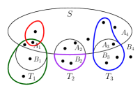
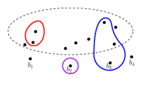
Figure 3: Construction of the set systems $(X,\mathcal{F}_{a})$ (middle) and $(Y,\mathcal{F}_{b})$ (right) given the set system on the left and $S,T_{1},T_{2},T_{3}$. The purple set can be added to either $(X_{,}\mathcal{F}_{a})$ or $(Y,\mathcal{F}_{b})$.

Otherwise, there exists a set $S$ with $5k<|S|<n-5k$. For $i=1,2,\ldots,k-1$, while there exists a set $T_{i}\in\mathcal{F}$ such that the Venn diagram $\textup{Venn}(S,T_{1},T_{2},\ldots,T_{i})$ on the $i+1$ sets contains at least $2(i+1)$ atoms, choose an arbitrary such set $T_{i}$. Suppose this process continues until the index $i$ reaches value $\ell\in[k-1]$. If $\ell=k-1$, then $\textup{Venn}(S,T_{1},\ldots,T_{\ell})$ is composed of $k$ sets and has at least $2k$ atoms, which cannot happen by assumption. Therefore, $\ell<k-1$. We say that a set $F$ cuts another set $F^{\prime}$ if both the regions $F\cap F^{\prime}$ and $F^{\prime}\setminus F$ are non-empty. By our stopping condition, every set $F\in\mathcal{F}$ cuts at most one atom in $\textup{Venn}(S,T_{1},\ldots,T_{\ell})$; indeed, if a set $F$ cuts two atoms or more, we would have added it as $T_{\ell+1}$ and continued.

Let the atoms of $\textup{Venn}(S,T_{1},\ldots,T_{\ell})$ inside $S$ be $A_{1},\ldots,A_{i}$, so that $A_{1}\cup\ldots\cup A_{i}=S$; and let the atoms outside $S$ be $B_{1},\ldots,B_{j}$, so that $B_{1}\cup\ldots\cup B_{j}=U\setminus S$. Define two new collections of elements $E_{a}:=\{a_{1},\ldots,a_{i}\}$ and $E_{b}:=\{b_{1},\ldots,b_{j}\}$, and define $X:=S\cup E_{b}$ and $Y:=(U\setminus S)\cup E_{a}$. We build two set systems $(X,\mathcal{F}_{a})$ and $(Y,\mathcal{F}_{b})$ as follows (see Figure 3). Initialize $\mathcal{F}_{a}=\mathcal{F}_{b}:=\varnothing$; for each set $F\in\mathcal{F}$, we have three cases:

1. If $F$ cuts an atom $A_{h}$ inside $S$, then add the set $(F\cap S)\cup\{b_{h}\mid h\in[j],F\supseteq B_{h}\}$ into $\mathcal{F}_{a}$.

2. Else, if $F$ cuts an atom $B_{h}$ outside $S$, then add the set $(F\setminus S)\cup\{a_{h}\mid h\in[i],F\supseteq A_{h}\}$ into $\mathcal{F}_{b}$.

3. Else, $F$ does not cut any atom. Execute either step (1) or step (2).

Here’s another equivalent way to look at this process. For $\mathcal{F}_{a}$, we can think taking the set system $(U,\mathcal{F})$, removing the sets that cut an atom outside $S$, and then contracting the atoms $B_{1},\ldots,B_{j}$ into $b_{1},\ldots,b_{j}$, respectively. We can also think of $\mathcal{F}_{b}$ analogously, by throwing away the sets that cut atoms inside $S$, and then contacting atoms $A_{1},\ldots,A_{i}$. Through this contraction viewpoint, it is clear that if the set system $(U,\mathcal{F})$ satisfy conditions (i) and (ii), then so do the set systems $(X,\mathcal{F}_{a})$ and $(Y,\mathcal{F}_{b})$. Moreover, since $5k<|S|<n-5k$, we have

$$|X|=|S|+|E_{b}|\leq|S|+2k\leq(n-5k)+2k<|U|$$

and

$$|Y|=|V\setminus S|+|E_{a}|\leq n-|S|+2k\leq(n-5k)+2k<|U|,$$

so we can apply induction on $n$, obtaining

$$|\mathcal{F}| =|\mathcal{F}_{a}|+|\mathcal{F}_{b}|$$

$$\leq\textup{ex}(n-|S|+2k)+\textup{ex}(|S|+2k)$$

$$\leq 10s\cdot k(5k+2)\cdot\mathsf{sf}(5k,r)\cdot\Big{(}\max\{1,(n-|S|+2k)-4k\}+\max\{1,(|S|+2k)-4k\}\Big{)}$$

$$=10s\cdot k(5k+2)\cdot\mathsf{sf}(5k,r)\cdot\Big{(}(n-|S|+2k)-4k+(|S|+2k)-4k\Big{)}$$

$$=10s\cdot k(5k+2)\cdot\mathsf{sf}(5k,r)\cdot(n-4k)=\textup{ex}(n),$$

completing the induction. ∎

Later when we apply the above lemma to $k$-cut, the number of atoms becomes $k$, so it is sufficient for even $k$. For odd $k$, we can slightly strengthen Lemma 14 as follows.

Corollary 15.

Let $\mathcal{F}$ be a set system on $n$ elements satisfying the following:

1. There do not exist sets $S_{1},\ldots,S_{k-1}$ such that $\textup{Venn}(S_{1},\ldots,S_{k-1})$ has at least $2(k-1)+1$ atoms.

2. There do not exist sets $S_{1},\ldots,S_{k}$ such that $\textup{Venn}(S_{1},\ldots,S_{k-1})$ has exactly $2(k-1)$ atoms, and the set $S_{k}$ cuts at least two atoms in $\textup{Venn}(S_{1},\ldots,S_{k-1})$.

3. Each of $\mathcal{F}$ and $\overline{\mathcal{F}}$ does not contain $s$ many $r$-sunflowers, each with distinct, nonempty cores.

Then, $|\mathcal{F}|\leq 10s\cdot k(5k+2)\cdot\mathsf{sf}(5k,r)\cdot n$.

Proof.

The proof is identical; the only additional observation is that when we iteratively construct $S,T_{1},\ldots,T_{\ell}$ for $\ell\leq k-1$, observe that the set $T_{\ell}$ cuts at least two atoms of $\textup{Venn}(S,T_{1},\ldots,T_{\ell-1})$ by construction. In particular, if the construction continued until $\ell=k-1$, then either the sets $S,T_{1},\ldots,T_{k-2}$ violate condition (i), or the sets $S,T_{1},\ldots,T_{k-1}$ violate condition (i’). Therefore, every time we carry out this process, we must stop at $\ell<k-1$. When we stop, the condition (i), though it is slightly more relaxed than the condition (i) of Lemma 14, still ensures that $|E_{a}|,|E_{b}|\leq 2k$, so the same inductive argument works. ∎

3.3 Relating Cuts and Sunflowers

Recall that $\overline{\lambda}_{k}$ is the size of the minimum $k$-cut divided by $k$, and $\gamma\in[1,2)$ is a fixed parameter. In this section, we use the previous tools for sunflowers to bound the number of small cuts (of size $\leq\gamma\overline{\lambda}_{k}$) in a graph. First, the following lemma, independent of sunflowers, shows that there cannot be many tiny cuts (of size $<\overline{\lambda}_{k}$) in a graph.

Lemma 16.

There are at most $2^{k-1}$ many cuts with weight less than $\overline{\lambda}_{k}$.

Proof.

Suppose, otherwise, that there are more than $2^{k-1}$ sets; let $\mathcal{S}$ be the collection of these sets. We will iteratively construct a $k$-cut of size less than $k\overline{\lambda}_{k}=\lambda_{k}$ contradicting the definition of $\lambda_{k}$, the size of the minimum $k$-cut.

Begin with an arbitrary set $S_{1}\in\mathcal{S}$, and while $\textup{Venn}(S_{1},\ldots,S_{i-1})$ has less than $k$ components, choose an arbitrary set $S_{i}\in\mathcal{S}$ such that $\textup{Venn}(S_{1},\ldots,S_{i})$ has at least one more component than $\textup{Venn}(S_{1},\ldots,S_{i-1})$. We show that such a set $S_{i}$ always exists. Let $A_{1},\ldots,A_{\ell}$ be the atoms of $\textup{Venn}(S_{1},\ldots,S_{i-1})$; the only sets $T\in\mathcal{S}$ such that $\textup{Venn}(S_{1},\ldots,S_{i-1},T)$ has the same number of components as $\textup{Venn}(S_{1},\ldots,S_{i-1})$ are sets of the form $\bigcup_{i\in I}A_{i}$ for some subset $I\subseteq[\ell]$. Since there are at most $2^{\ell}\leq 2^{k-1}$ such sets and $|\mathcal{S}|>2^{k-1}$, a satisfying set $S_{i}$ always exists.

At the end, we have at most $k-1$ sets $S_{1},\ldots,S_{i}$ such that $\textup{Venn}(S_{1},\ldots,S_{i})$ has at least $k$ components. Therefore, the edge set $\partial S_{1}\cup\cdots\cup\partial S_{i}$ is a $k$-cut, and it has weight less than $i\overline{\lambda}_{k}<k\overline{\lambda}_{k}=\lambda_{k}$, achieving the desired contradiction. ∎

Finally, the following lemma proves that many sunflowers consisting of cuts of size $\leq\gamma\overline{\lambda}_{k}$ will lead to a better $k$-cut than $k\overline{\lambda}_{k}$, leading to contradiction.

Lemma 17.

Fix a constant $1\leq\gamma<2$, and let $\mathcal{F}$ be the family of sets $\{S\subseteq V:w(\partial S)\leq\gamma\overline{\lambda}_{k}\}$. Then, for any $r>\frac{2\gamma}{2-\gamma}+1$, both $\mathcal{F}$ and $\overline{\mathcal{F}}$ do not contain $2^{k}$ many $(r+k-2)$-sunflowers with distinct, nonempty cores.

Proof.

Since $w(\partial S)\leq\gamma\overline{\lambda}_{k}\iff w(\partial(V\setminus S))\leq\gamma\overline{\lambda}_{k}$, we have $\mathcal{F}=\overline{\mathcal{F}}$, so it suffices to only consider $\mathcal{F}$. Suppose, otherwise, that there are $2^{k}$ many $(r+k-2)$-sunflowers with distinct, nonempty cores. Let $\mathcal{F}_{\textup{small}}:=\{S\mid\varnothing\subsetneq S\subsetneq V,\,w(\partial S)<\overline{\lambda}_{k}\}$, so that Lemma 16 implies that $|\mathcal{F}_{\textup{small}}|\leq 2^{k-1}$. Then, there must exist at least one sunflower in this collection whose core does not belong to $\mathcal{F}_{\textup{small}}$. Let $S_{1},\ldots,S_{r+k-2}\in\mathcal{F}$ be the sets of this $(r+k-2)$-sunflower with petals $P_{i}:=S_{i}\setminus\bigcup_{j\neq r}S_{j}$ and nonempty core $C:=\bigcap_{i}S_{i}\notin\mathcal{F}_{\textup{small}}$. Since the petals $P_{i}$ are disjoint, at most $k-2$ of them are in $\mathcal{F}_{\textup{small}}$, since otherwise, we get $k-1$ disjoint sets in $\mathcal{F}_{\textup{small}}$ which together form a $k$-cut with weight less than $(k-1)\overline{\lambda}_{k}<\lambda_{k}$. Therefore, without loss of generality (by reordering the sets $S_{i}$), assume that $P_{1},\ldots,P_{r}\notin\mathcal{F}_{\textup{small}}$. Since $C$ and $P_{1},\ldots,P_{r}$ are all cuts in the graph (in particular, $\varnothing\neq C\neq V$ and $\varnothing\neq P_{i}\neq V$) and are not in $\mathcal{F}_{\textup{small}}$, we have $w(\partial C)\geq\overline{\lambda}_{k}$ and $w(\partial P_{i})\geq\overline{\lambda}_{k}$ for each $i\in[r]$. For each $i\in[r]$, we have

$$\gamma\overline{\lambda}_{k}\geq w(\partial S_{i})=w(\partial(C\cup P_{i}))=w(\partial C)+w(\partial P_{i})-2w(E[C,P_{i}])\geq 2\overline{\lambda}_{k}-2w(E[C,P_{i}]),$$

so $w(E[C,P_{i}])\geq(2-\gamma)\overline{\lambda}_{k}/2$. Now observe that the edges in $E[C,P_{i}]$ for $i=2,\ldots,r$ are included in $\partial(C\cup P_{1})$. It follows that

$$\gamma\overline{\lambda}_{k}\geq w(\partial(C\cup P_{1}))\geq w(E[C,P_{2}]\cup\cdots\cup E[C,P_{r}])=\sum_{i=2}^{r}w(E[C,P_{i}])\geq(r-1)\frac{(2-\gamma)\overline{\lambda}_{k}}{2},$$

so $r-1\leq\frac{2\gamma}{2-\gamma}$, contradicting the assumption that $r>\frac{2\gamma}{2-\gamma}+1$. ∎

We are finally ready to prove Theorem 10, which we restate here for convenience.

See 10

Proof.

Let $\mathcal{F}$ be the set of such cuts, and let $k^{\prime}:=\lceil k/2\rceil$. We first show that if $k$ is even, then condition (i) of Lemma 14 is satisfied when the parameter $k$ in the lemma is $k^{\prime}$ instead, and if $k$ is odd, then conditions (i) and (i’) of Corollary 15 are satisfied, again with $k^{\prime}$ for the parameter $k$. Then, we show that condition (ii) of both Lemma 14 and Corollary 15 are satisfied for parameters $s$ and $r$ that we choose later.

First, consider the case when $k$ is even. Suppose, otherwise, that condition (i) of Lemma 14 is false: there are sets $S_{1},\ldots,S_{k^{\prime}}$ such that $\textup{Venn}(S_{1},\ldots,S_{k^{\prime}})$ has at least $2k^{\prime}=k$ atoms. Then, $\partial S_{1}\cup\cdots\cup\partial S_{k^{\prime}}$ is a $k$-cut with weight $k^{\prime}\cdot\gamma\overline{\lambda}_{k}<\frac{k}{2}\cdot 2\overline{\lambda}_{k}=\lambda_{k}$, contradicting the definition of $\lambda_{k}$, the minimum $k$-cut.

Now consider the case when $k$ is odd. If condition (i) of Corollary 15 is false, then there are sets $S_{1},\ldots,S_{k^{\prime}-1}$ such that $\textup{Venn}(S_{1},\ldots,S_{k^{\prime}}$ has at least $2(k^{\prime}-1)-1=k$ atoms. Then, $\partial S_{1}\cup\cdots\cup\partial S_{k^{\prime}-1}$ is a $k$-cut with weight $(k^{\prime}-1)\cdot\gamma\overline{\lambda}_{k}<\frac{k}{2}\cdot 2\overline{\lambda}_{k}=\lambda_{k}$, contradicting the definition of $\lambda_{k}$, the minimum $k$-cut. Otherwise, if condition (i’) of Corollary 15 is false, then the set of edges $\partial S_{1}\cup\cdots\cup\partial S_{k^{\prime}-1}$ is a $(k-1)$-cut with weight $(k^{\prime}-1)\cdot\gamma\overline{\lambda}_{k}<\frac{k-1}{2}\cdot 2\overline{\lambda}_{k}=(k-1)\overline{\lambda}_{k}$. Let $A_{1},\ldots,A_{\ell}\subseteq V$ be the atoms in $\textup{Venn}(S_{1},\ldots,S_{k^{\prime}-1})$ that are cut by $S_{k^{\prime}}$, with $\ell\geq 2$ by assumption. Since $\partial S_{k^{\prime}}\cap E[A_{i}]$ are disjoint for $i\in[\ell]$, there exists one atom $A_{i}$ such that

$$w(\partial S_{k^{\prime}}\cap E[A_{i}])\leq\frac{1}{\ell}w(\partial S_{k^{\prime}})\leq\frac{1}{\ell}\cdot\gamma\overline{\lambda}_{k}<\frac{1}{2}\cdot 2\overline{\lambda}_{k}=\overline{\lambda}_{k}.$$

Thus, $\partial S_{1}\cup\cdots\cup\partial S_{k^{\prime}-1}\cup(\partial S_{k^{\prime}}\cap E[A_{i}])$ is a $k$-cut with weight less than $(k-1)\overline{\lambda}_{k}+\overline{\lambda}_{k}=\overline{\lambda}_{k}$, a contradiction. Thus, conditions (i) and (i’) of Corollary 15 are satisfied.

Now, fix the parameters $s:=2^{k}$, $r:=\lceil\frac{2\gamma}{2-\gamma}+2\rceil$, $r^{\prime}:=r+k-2$, and $k^{\prime}:=\lceil k/2\rceil$. By Lemma 17, both $\mathcal{F}$ and $\overline{\mathcal{F}}$ do not contain $s$ many $r^{\prime}$-sunflowers with distinct, nonempty cores, fulfilling condition (ii) of Lemma 14 and Corollary 15 (with $r^{\prime}$ in place of $r$). Therefore, by Lemma 14 or Corollary 15 when $k$ is even or odd respectively, and using $\mathsf{sf}(d,r)\leq(\lg d)^{d}(r\cdot\lg\lg d)^{O(d)}\leq(r\lg d\lg\lg d)^{O(d)}$ [ALWZ19],

$$|\mathcal{F}| \leq 10s\cdot k^{\prime}(5k^{\prime}+2)\cdot\mathsf{sf}(5k^{\prime},r^{\prime})\cdot n\leq 2^{O(k)}\cdot(r^{\prime}\lg k^{\prime}\lg\lg k^{\prime})^{O(k^{\prime})}n$$

$$=2^{O(k)}\cdot\left(\left(\lceil\frac{2\gamma}{2-\gamma}\rceil+k\right)\lg k^{\prime}\lg\lg k^{\prime}\right)^{O(k^{\prime})}\cdot n\leq\left(\max\left(\frac{1}{2-\gamma},k\right)\right)^{O(k)}\cdot n$$

as desired. As an aside, using the classical Erdős-Rado bound [ER60] of $\mathsf{sf}(d,r)\leq d!(r-1)^{d}$ gives the same result, up to a constant in the $O(k)$ exponent, as does the conjectured optimal bound of $\mathsf{sf}(d,f)\leq(Cr)^{d}$. ∎

Appendix A Omitted Proofs

Proof of Claim 5.

We have

$$\tilde{f}(0)=\frac{1}{1-A}n(1-A)=n=f(0)$$

and

$$\tilde{f}^{\prime}(t) =\frac{1}{1-A}n(-\frac{\gamma}{2}e^{-(\gamma/2)t}+Ae^{-t})$$

$$=\frac{1}{1-A}n\left(-\frac{\gamma}{2}e^{-(\gamma/2)t}+\frac{\gamma}{2}Ae^{-t}+\left(A-\frac{\gamma}{2}A\right)e^{-t}\right)$$

$$=-\frac{\gamma}{2}\cdot\frac{1}{1-A}n(e^{-(\gamma/2)t}-Ae^{-t})+\frac{A-(\gamma/2)A}{1-A}e^{-t}n$$

$$=-\frac{\gamma}{2}\tilde{f}(t)+\frac{A-(\gamma/2)A}{1-A}e^{-t}n.$$

$$=-\frac{\gamma}{2}\tilde{f}(t)+Be^{-t}n,$$

where the last equality holds because

$$A=\frac{B}{B+1-\gamma/2} \iff BA+A-\frac{\gamma}{2}A=B$$

$$\iff A-\frac{\gamma}{2}A=B-BA=B(1-A)$$

$$\iff\frac{A-(\gamma/2)A}{1-A}=B.$$

Since $\tilde{f}(0)=f(0)$ and $\tilde{f}(t)$ satisfies (2) with equality, we have $\tilde{f}(t)\geq f(t)$ for all $t\geq 0$. ∎

References

- [ALWZ19] Ryan Alweiss, Shachar Lovett, Kewen Wu, and Jiapeng Zhang. Improved bounds for the sunflower lemma. arXiv preprint arXiv:1908.08483, 2019.
- [CQX18] Chandra Chekuri, Kent Quanrud, and Chao Xu. LP relaxation and tree packing for minimum k-cuts. In 2nd Symposium on Simplicity in Algorithms (SOSA 2019). Schloss Dagstuhl-Leibniz-Zentrum fuer Informatik, 2018.
- [ER60] P. Erdős and R. Rado. Intersection theorems for systems of sets. J. London Math. Soc., 35:85–90, 1960.
- [Fre75] David A Freedman. On tail probabilities for martingales. the Annals of Probability, 3(1):100–118, 1975.
- [GH94] Olivier Goldschmidt and Dorit S. Hochbaum. A polynomial algorithm for the -cut problem for fixed . Math. Oper. Res., 19(1):24–37, 1994.
- [GLL18] Anupam Gupta, Euiwoong Lee, and Jason Li. Faster exact and approximate algorithms for -cut. In Foundations of Computer Science (FOCS), 2018 IEEE 59th Annual Symposium on, 2018.
- [GLL19] Anupam Gupta, Euiwoong Lee, and Jason Li. The number of minimum k-cuts: improving the karger-stein bound. In Proceedings of the 51st Annual ACM SIGACT Symposium on Theory of Computing, pages 229–240. ACM, 2019.
- [KS96] David R. Karger and Clifford Stein. A new approach to the minimum cut problem. Journal of the ACM (JACM), 43(4):601–640, 1996.
- [KYN07] Yoko Kamidoi, Noriyoshi Yoshida, and Hiroshi Nagamochi. A deterministic algorithm for finding all minimum -way cuts. SIAM J. Comput., 36(5):1329–1341, 2006/07.
- [Li19] Jason Li. Faster minimum k-cut of a simple graph. In Foundations of Computer Science (FOCS), 2019 IEEE 60th Annual Symposium on, 2019.
- [NI92] Hiroshi Nagamochi and Toshihide Ibaraki. Computing edge-connectivity in multigraphs and capacitated graphs. SIAM J. Discrete Math., 5(1):54–66, 1992.
- [Tho08] Mikkel Thorup. Minimum -way cuts via deterministic greedy tree packing. In Proceedings of the fortieth annual ACM symposium on Theory of computing, pages 159–166. ACM, 2008.