Random Fourier Features via Fast Surrogate Leverage Weighted Sampling

Abstract

In this paper, we propose a fast surrogate leverage weighted sampling strategy to generate refined random Fourier features for kernel approximation. Compared to the current state-of-the-art method that uses the leverage weighted scheme (?), our new strategy is simpler and more effective. It uses kernel alignment to guide the sampling process and it can avoid the matrix inversion operator when we compute the leverage function. Given $n$ observations and $s$ random features, our strategy can reduce the time complexity for sampling from $\mathcal{O}(ns^{2}+s^{3})$ to $\mathcal{O}(ns^{2})$, while achieving comparable (or even slightly better) prediction performance when applied to kernel ridge regression (KRR). In addition, we provide theoretical guarantees on the generalization performance of our approach, and in particular characterize the number of random features required to achieve statistical guarantees in KRR. Experiments on several benchmark datasets demonstrate that our algorithm achieves comparable prediction performance and takes less time cost when compared to (?).

1 Introduction

Kernel methods (?) are one of the most important and powerful tools in statistical learning. However, kernel methods often suffer from scalability issues in large-scale problems due to high space and time complexities. For example, given $n$ observations in the original $d$-dimensional space $\mathcal{X}$, kernel ridge regression (KRR) requires $\mathcal{O}(n^{3})$ training time and $\mathcal{O}(n^{2})$ space to store the kernel matrix, which becomes intractable when $n$ is large.

One of the most popular approaches for scaling up kernel methods is random Fourier features (RFF) (?), which approximates the original kernel by mapping input features into a new space spanned by a small number of Fourier basis. Specifically, suppose a given kernel $k(\cdot,\cdot):\mathcal{X}\times\mathcal{X}\rightarrow\mathbb{R}$ satisfies 1) positive definiteness and 2) shift-invariance, i.e., $k(\bm{x},\bm{x}^{\prime})=k(\bm{x}-\bm{x}^{\prime})$. By Bochner’s theorem (?), there exists a finite Borel measure $p(\bm{w})$ (the Fourier transform associated with $k$) such that

$$\begin{split}k(\bm{x}-\bm{x}^{\prime})&=\int_{\mathbb{R}^{d}}p(\bm{w})\exp\big{(}\mbox{i}\bm{w}^{\!\top}(\bm{x}-\bm{x}^{\prime})\big{)}\mbox{d}\bm{w}\,.\end{split}$$ (1)

(Typically, the kernel is real-valued and thus the imaginary part in Eq. (1) can be discarded.) One can then use Monte Carlo sampling to approximate $k(\bm{x},\bm{x}^{\prime})$ by the low-dimensional kernel $\tilde{k}_{p}(\bm{x},\bm{x}^{\prime})=\varphi_{p}(\bm{x})^{\!\top}\varphi_{p}(\bm{x}^{\prime})$ with the explicit mapping

$$\varphi_{p}(\bm{x})\!:=\!\frac{1}{\sqrt{s}}\big{[}\exp(-\mbox{i}\bm{w}^{\!\top}_{1}\bm{x}),\cdots,\exp(-\mbox{i}\bm{w}^{\!\top}_{s}\bm{x})]^{\!\top}\,,$$ (2)

where $\{\bm{w}_{i}\}_{i=1}^{s}$ are sampled from $p(\bm{w})$ independently of the training set. For notational simplicity, here we write $z_{p}(\bm{w}_{i},\bm{x}_{j}):=1/\sqrt{s}\exp(-\mbox{i}\bm{w}^{\!\top}_{i}\bm{x}_{j})$ such that $\varphi_{p}(\bm{x})=[z_{p}(\bm{w}_{1},\bm{x}),\cdots,z_{p}(\bm{w}_{s},\bm{x})]^{\!\top}$. Note that we have $k(\bm{x},\bm{x}^{\prime})=\mathbb{E}_{\bm{w}\sim p}[\varphi_{p}(\bm{x})^{\!\top}\varphi_{p}(\bm{x}^{\prime})]\approx\tilde{k}_{p}(\bm{x},\bm{x}^{\prime})=\sum_{i=1}^{s}z_{p}(\bm{w}_{i},\bm{x})z_{p}(\bm{w}_{i},\bm{x}^{\prime})$. Consequently, the original kernel matrix $\bm{K}=[k(\bm{x}_{i},\bm{x}_{j})]_{n\times n}$ on the $n$ observations $\bm{X}=\{\bm{x}_{i}\}_{i=1}^{n}$ can be approximated by $\bm{K}\approx\tilde{\bm{K}}_{p}=\bm{Z}_{p}\bm{Z}_{p}^{\!\top}$, where $\bm{Z}_{p}=[\varphi_{p}(\bm{x}_{1}),\cdots,\varphi_{p}(\bm{x}_{n})]^{\!\top}\in\mathbb{R}^{n\times s}$. With $s$ random features, this approximation applied to KRR only requires $\mathcal{O}(ns^{2})$ time and $\mathcal{O}(ns)$ memory, hence achieving a substantial computational saving when $s\ll n$.

Since RFF uses the Monte Carlo estimates that are independent of the training set, a large number of random features are often required to achieve competitive approximation and generalization performance. To improve performance, recent works (?; ?) consider using the ridge leverage function (?; ?) defined with respect to the training data. For a given random feature $\bm{w}_{i}$, this function is defined as

$$l_{\lambda}(\bm{w}_{i})=p(\bm{w}_{i})\bm{z}^{\!\top}_{p,\bm{w}_{i}}(\bm{X})(\bm{K}+n\lambda\bm{I})^{-1}\bm{z}_{p,\bm{w}_{i}}(\bm{X})\,,$$ (3)

where $\lambda$ is the regularization parameter in KRR and $\bm{z}_{p,\bm{w}_{i}}(\bm{X})\in\mathbb{R}^{n}$ is the $i$-th column of $\bm{Z}_{p}$ given by $(\bm{z}_{p,\bm{w}_{i}}(\bm{X}))_{j}:=z_{p}(\bm{w}_{i},\bm{x}_{j})$. Observe that $q^{*}(\bm{w}):=\frac{l_{\lambda}(\bm{w})}{\int l_{\lambda}(\bm{w})\text{d}\bm{w}}$ can be viewed as a probability density function, and hence is referred to as the Empirical Ridge Leverage Score (ERLS) distribution (?). Therefore, one can sample the features $\{\bm{w}_{i}\}_{i=1}^{s}$ according to $q^{*}(\bm{w})$, which is an importance weighted sampling strategy. Compared to standard Monte Carlo sampling for RFF, $q^{*}(\bm{w})$-based sampling requires fewer Fourier features and enjoys theoretical guarantees (?; ?).

However, computing the ridge leverage scores and the ERLS distribution may be intractable when $n$ is large, as we need to invert the kernel matrix in Eq. (3). An alternative way in (?; ?) is to use the subset of data to approximate $\bm{K}$, but this scheme still needs $\mathcal{O}(ns^{2}+s^{3})$ time to generate random features. To address these computational difficulties, we design a simple but effective leverage function to replace the original one. For a given $\bm{w}$, our leverage function is defined as

$$L_{\lambda}(\bm{w})=p(\bm{w})\bm{z}^{\!\top}_{p,\bm{w}}(\bm{X})\left(\frac{1}{n^{2}\lambda}\Big{(}\bm{y}\bm{y}^{\!\top}+n\bm{I}\Big{)}\right)\bm{z}_{p,\bm{w}}(\bm{X})\,,$$ (4)

where the matrix $\bm{y}\bm{y}^{\!\top}$ is an ideal kernel that directly fits the training data with 100% accuracy in classification tasks, and thus can be used to guide kernel learning tasks as in kernel alignment (?). It can be found that, our surrogate function avoids the matrix inversion operator so as to further accelerate kernel approximation. Note that, we introduce the additional term $n\bm{I}$ and the coefficient $1/(n^{2}\lambda)$ in Eq. (4) to ensure, $L_{\lambda}$ is a surrogate function that upper bounds $l_{\lambda}$ in Eq. (3) for theoretical guarantees. This can be achieved due to $L_{\lambda}(\bm{w}_{i})\geq l_{\lambda}(\bm{w}_{i})$. In this way, our method with the surrogate function requires less computational time while achieving comparable generalization performance, as demonstrated by our theoretical results and experimental validations.

Specifically, the main contributions of this paper are:

• We propose a surrogate ridge leverage function based on kernel alignment and derive its associated fast surrogate ERLS distribution. This distribution is simple in form and has intuitive physical meanings. Our theoretical analysis provides a lower bound on the number of random features that guarantees no loss in the learning accuracy in KRR.

• By sampling from the surrogate ERLS distribution, our data-dependent algorithm takes $\mathcal{O}(ns^{2})$ time to generate random features, which is the same as RFF and less than the $\mathcal{O}(ns^{2}+s^{3})$ time in (?). We further provide theoretical guarantees on the generalization performance of our algorithm equipped with the KRR estimator.

• Experiments on various benchmark datasets demonstrate that our method performs better than standard random Fourier features based algorithms. Specifically, our algorithm achieves comparable (or even better) accuracy and uses less time when compared to (?).

The remainder of the paper is organized as follows. Section 2 briefly reviews the related work on random features for kernel approximation. Our surrogate leverage weighted sampling strategy for RFF is presented in Section 3, and related theoretical results are given in Section 4. In section 5, we provide experimental evaluation for our algorithm and compare with other representative random features based methods on popular benchmarks. The paper is concluded in Section 6.

2 Related Works

Recent research on random Fourier features focuses on constructing the mapping

$$\varphi(\bm{x}):=\frac{1}{\sqrt{s}}\big{[}a_{1}\exp(-\mbox{i}\bm{w}^{\!\top}_{1}\bm{x}),\cdots,a_{s}\exp(-\mbox{i}\bm{w}^{\!\top}_{s}\bm{x})]^{\!\top}\,.$$

The key question is how to select the points $\bm{w}_{i}$ and weights $a_{i}$ so as to uniformly approximate the integral in Eq. (1). In standard RFF, $\{\bm{w}_{i}\}_{i=1}^{s}$ are randomly sampled from $p(\bm{w})$ and the weights are equal, i.e., $a_{i}\equiv 1$. To reduce the approximation variance, ? (?) proposes the orthogonal random features (ORF) approach, which incorporates an orthogonality constraint when sampling $\{\bm{w}_{i}\}_{i=1}^{s}$ from $p(\bm{w})$. Sampling theory ? (?) suggests that the convergence of Monte-Carlo used in RFF and ORF can be significantly improved by choosing a deterministic sequence $\{\bm{w}_{i}\}$ instead of sampling randomly. Therefore, a possible middle-ground method is Quasi-Monte Carlo sampling (?), which uses a low-discrepancy sequence $\{\bm{w}_{i}\}$ rather than the fully random Monte Carlo samples. Other deterministic approaches based on numerical quadrature are considered in (?). ? (?) analyzes the relationship between random features and quadrature, which allows one to use deterministic numerical integration methods such as Gaussian quadrature (?), spherical-radial quadrature rules (?), and sparse quadratures (?) for kernel approximation.

The above methods are all data-independent, i.e., the selection of points and weights is independent of the training data. Another line of work considers data-dependent algorithms, which use the training data to guide the generation of random Fourier features by using, e.g., kernel alignment (?), feature compression (?), or the ridge leverage function (?; ?; ?; ?). Since our method builds on the leverage function $l_{\lambda}(\bm{w})$, we detail this approach here. From Eq. (3), the integral of $l_{\lambda}(\bm{w})$ is

$$\int_{\mathbb{R}^{d}}l_{\lambda}(\bm{w})\mbox{d}\bm{w}=\operatorname{Tr}\left[\bm{K}(\bm{K}+n\lambda\bm{I})^{-1}\right]=:d_{\bm{K}}^{\lambda}\,.$$ (5)

The quantity $d_{\bm{K}}^{\lambda}\ll n$ determines the number of independent parameters in a learning problem and hence is referred to as the number of effective degrees of freedom (?). ? (?) provides the sharpest bound on the required number of random features; in particular, with $\Omega(\sqrt{n}\log d_{\bm{K}}^{\lambda})$ features, no loss is incurred in learning accuracy of kernel ridge regression. Albeit elegant, sampling according to $q^{*}(\bm{w})$ is often intractable in practice. The alternative approach proposed in (?) takes $\mathcal{O}(ns^{2}+s^{3})$ time, which is larger than $\mathcal{O}(ns^{2})$ in the standard RFF.

3 Surrogate Leverage Weighted RFF

3.1 Problem setting

Consider a standard supervised learning setting, where $\mathcal{X}$ is a compact metric space of features, and $\mathcal{Y}\subseteq\mathbb{R}$ (in regression) or $\mathcal{Y}=\{-1,1\}$ (in classification) is the label space. We assume that a sample set $\{(\bm{x}_{i},y_{i})\}_{i=1}^{n}$ is drawn from a non-degenerate Borel probability measure $\rho$ on $\mathcal{X}\times\mathcal{Y}$. The target function of $\rho$ is defined by $f_{\rho}(\bm{x}):=\int_{\mathcal{Y}}y\mathrm{d}\rho(y|\bm{x})$ for each $\bm{x}\in\mathcal{X}$, where $\rho(\cdot|\bm{x})$ is the conditional distribution of $\rho$ at $\bm{x}$. Given a kernel function $k$ and its associated reproducing kernel Hilbert space (RKHS) $\mathcal{H}$, the goal is to find a hypothesis $f:\mathcal{X}\rightarrow\mathcal{Y}$ in $\mathcal{H}$ such that $f(\bm{x})$ is a good estimate of the label $y\in\mathcal{Y}$ for a new instance $\bm{x}\in\mathcal{X}$. By virtue of the representer theorem (?), an empirical risk minimization problem can be formulated as

$$\hat{f}^{\lambda}:=\underset{f\in\mathcal{H}}{\operatorname*{argmin}}~{}\frac{1}{n}\sum_{i=1}^{n}\ell\left(y_{i},f(\bm{x}_{i})\right)+\lambda\bm{\alpha}^{\!\top}\bm{K}\bm{\alpha}\,,$$ (6)

where $f=\sum_{i=1}^{n}\alpha_{i}k(\bm{x}_{i},\cdot)$ with $\bm{\alpha}\in\mathbb{R}^{n}$ and the convex loss $\ell:\mathcal{Y}\times\mathcal{Y}\rightarrow\mathbb{R}$ quantifies the quality of the estimate $f(\bm{x})$ w.r.t. the true $y$. In this paper, we focus on learning with the squared loss, i.e., $\ell(y,f(\bm{x}))=(y-f(\bm{x}))^{2}$. Hence, the expected risk in KRR is defined as $\mathcal{E}(f)=\int_{\mathcal{X}\times\mathcal{Y}}(f(\bm{x})-y)^{2}\mathrm{d}\rho$, with the corresponding empirical risk defined on the sample, i.e., $\hat{\mathcal{E}}(f)=\frac{1}{n}\sum_{i=1}^{n}\big{(}f(\bm{x}_{i})-y_{i}\big{)}^{2}$. In standard learning theory, the optimal hypothesis $f_{\rho}$ is defined as $f_{\rho}(\bm{x})=\int_{Y}y\mathrm{d}\rho(y|\bm{x}),\quad\bm{x}\in\mathcal{X}$, where $\rho(\cdot|\bm{x})$ is the conditional distribution of $\rho$ at $\bm{x}\in\mathcal{X}$. The regularization parameter $\lambda$ in Eq. (6) should depend on the sample size; in particular, $\lambda\equiv\lambda(n)$ with $\lim_{n\rightarrow\infty}\lambda(n)=0$. Following (?; ?), we pick $\lambda\in\mathcal{O}(n^{-1/2})$.

As shown in (?), when using random features, the empirical risk minimization problem (6) can be expressed as

$$\bm{\beta}_{\lambda}:=\underset{\bm{\beta}\in\mathbb{R}^{s}}{\operatorname*{argmin}}~{}\frac{1}{n}\left\|\bm{y}-\bm{Z}_{q}\bm{\beta}\right\|_{2}^{2}+\lambda\|\bm{\beta}\|_{2}^{2}\,,$$ (7)

where $\bm{y}=[y_{1},y_{2},\cdots,y_{n}]^{\!\top}$ is the label vector and $\bm{Z}_{q}=[\varphi_{q}(\bm{x}_{1}),\cdots,\varphi_{q}(\bm{x}_{n})]^{\!\top}\in\mathbb{R}^{n\times s}$ is the random feature matrix, with $\varphi_{q}(\bm{x})$ as defined in Eq. (2) and $\{\bm{w}_{i}\}_{i=1}^{s}$ sampled from a distribution $q(\bm{w})$. Eq. (7) is a linear ridge regression problem in the space spanned by the random features (?; ?), and the optimal hypothesis is given by $\bm{f}_{\bm{\beta}}^{\lambda}=\bm{Z}_{q}\bm{\beta}_{\lambda}$, with

$$\bm{\beta}_{\lambda}=(\bm{Z}_{q}^{\!\top}\bm{Z}_{q}+n\lambda\bm{I})^{-1}\bm{Z}_{q}^{\!\top}\bm{y}\,.$$ (8)

Note that the distribution $q(\bm{w})$ determines the feature mapping matrix and hence has a significant impact on the generalization performance. Our main goal in the sequel is to design a good $q(\bm{w})$, and to understand the relationship between $q(\bm{w})$ and the expected risk. In particular, we would like to characterize the number $s$ of random features needed when sampling from $q(\bm{w})$ in order to achieve a certain convergence rate of the risk.

3.2 Surrogate leverage weighted sampling

Let $q(\bm{w})$ be a probability density function to be designed. Given the points $\{\bm{w}_{i}\}_{i=1}^{s}$ sampled from $q(\bm{w})$, we define the mapping

$$\varphi_{q}(\bm{x})=\frac{1}{\sqrt{s}}\left(\sqrt{\frac{p\left(\bm{w}_{1}\right)}{q\left(\bm{w}_{1}\right)}}e^{-\mbox{i}\bm{w}^{\!\top}_{1}\bm{x}},\cdots,\sqrt{\frac{p\left(\bm{w}_{s}\right)}{q\left(\bm{w}_{s}\right)}}e^{-\mbox{i}\bm{w}^{\!\top}_{s}\bm{x}}\right)^{\!\!\top}\,.$$ (9)

We again have $k(\bm{x},\bm{x}^{\prime})=\mathbb{E}_{\bm{w}\sim q}[\varphi_{q}(\bm{x})^{\!\top}\varphi_{q}(\bm{x}^{\prime})]\approx\tilde{k}_{q}(\bm{x},\bm{x}^{\prime})=\sum_{i=1}^{s}z_{q}(\bm{w}_{i},\bm{x})z_{q}(\bm{w}_{i},\bm{x}^{\prime})$, where $z_{q}(\bm{w}_{i},\bm{x}_{j}):=\sqrt{p(\bm{w}_{i})/q(\bm{w}_{i})}z_{p}(\bm{w}_{i},\bm{x}_{j})$. Accordingly, the kernel matrix $\bm{K}$ can be approximated by $\bm{K}_{q}=\bm{Z}_{q}\bm{Z}_{q}^{\!\top}$, where $\bm{Z}_{q}:=[\varphi_{q}(\bm{x}_{1}),\cdots,\varphi_{q}(\bm{x}_{n})]^{\!\top}\in\mathbb{R}^{n\times s}$. Denoting by $\bm{z}_{q,\bm{w}_{i}}(\bm{X})$ the $i$-th column of $\bm{Z}_{q}$, we have $\bm{K}=\mathbb{E}_{\bm{w}\sim p}[\bm{z}_{p,\bm{w}}(\bm{X})\bm{z}^{\!\top}_{p,\bm{w}}(\bm{X})]=\mathbb{E}_{\bm{w}\sim q}[\bm{z}_{q,\bm{w}}(\bm{X})\bm{z}^{\!\top}_{q,\bm{w}}(\bm{X})]$. Note that this scheme can be regarded as a form of importance sampling.

Our surrogate empirical ridge leverage score distribution $L_{\lambda}(\bm{w})$ is given by Eq. (4). The integral of $L_{\lambda}(\bm{w})$ is

$$\int_{\mathbb{R}^{d}}L_{\lambda}(\bm{w})\mbox{d}\bm{w}=\frac{1}{n^{2}\lambda}\operatorname{Tr}\left[\big{(}\bm{y}\bm{y}^{\!\top}\!\!+n\bm{I}\big{)}\bm{K}\right]:=D^{\lambda}_{\bm{K}}\,.$$ (10)

Combining Eq. (4) and Eq. (10), we can compute the surrogate empirical ridge leverage score distribution by

$$q(\bm{w}):=\frac{L_{\lambda}(\bm{w})}{\int_{\mathbb{R}^{d}}L_{\lambda}(\bm{w})\text{d}\bm{w}}=\frac{L_{\lambda}(\bm{w})}{D^{\lambda}_{\bm{K}}}\,.$$ (11)

The random features $\{\bm{w}_{i}\}_{i=1}^{s}$ can then be sampled from the above $q(\bm{w})$. We refer to this sampling strategy as surrogate leverage weighted RFF. Compared to the standard $l_{\lambda}$ and its associated ERLS distribution, the proposed $L_{\lambda}(\bm{w})$ and $D^{\lambda}_{\bm{K}}$ are simpler: it does not require inverting the kernel matrix and thus accelerates the generation of random features.

Since the distribution $q(\bm{w})$ involves the kernel matrix $\bm{K}$ that is defined on the entire training dataset, we need to approximate $\bm{K}$ by random features, and then calculate/approximate $q(\bm{w})$. To be specific, we firstly sample $\{\bm{w}_{i}\}_{i=1}^{l}$ with $l\geq s$ from the spectral measure $p(\bm{w})$ and form the feature matrix $\bm{Z}_{l}\in\mathbb{R}^{n\times l}$. We have $\bm{K}\approx\tilde{\bm{K}}_{p}=\bm{Z}_{l}\bm{Z}_{l}^{\!\top}$, and thus the distribution $q(\bm{w})$ can be approximated by

$$\tilde{q}(\bm{w})=\frac{p(\bm{w})\bm{z}^{\!\top}_{p,\bm{w}}(\bm{X})\left(\bm{y}\bm{y}^{\!\top}+n\bm{I}\right)\bm{z}_{p,\bm{w}}(\bm{X})}{\|\bm{y}^{\!\top}\!\bm{Z}_{l}\|_{2}^{2}+n\|\bm{Z}_{l}\|^{2}_{\text{F}}}\,.$$ (12)

Hence, we can then sample from $\tilde{q}(\bm{w})$ to generate the refined random features by importance sampling.

Note that the term $n\bm{I}$ in Eq. (4) and Eq. (12) is independent of the sample set $\bm{X}$. If we discard this term in our algorithm implementation, $L_{\lambda}(\bm{w})$ in Eq. (4) can be transformed as

$$L^{\prime}_{\lambda}(\bm{w})=p(\bm{w})\bm{z}^{\!\top}_{p,\bm{w}}(\bm{X})\left(\frac{1}{n^{2}\lambda}\bm{y}\bm{y}^{\!\top}\right)\bm{z}_{p,\bm{w}}(\bm{X})\,,$$ (13)

and further $\tilde{q}(\bm{w})$ in Eq. (12) can be simplified to

$$\tilde{q}^{\prime}(\bm{w})=\frac{p(\bm{w})\bm{z}^{\!\top}_{p,\bm{w}}(\bm{X})\left(\bm{y}\bm{y}^{\!\top}\right)\bm{z}_{p,\bm{w}}(\bm{X})}{\|\bm{y}^{\!\top}\!\bm{Z}_{l}\|_{2}^{2}}\,.$$ (14)

For each feature $\bm{w}_{i}\sim\tilde{q}^{\prime}(\bm{w})$, its re-sampling probability $p_{i}$ is associated with the approximate empirical ridge leverage score in Eq. (13). To be specific, it can be represented as

$$p_{i}\propto\left(\bm{y}^{\!\top}(\bm{Z}_{l})_{i}\right)^{2}=\bigg{|}\sum_{j=1}^{n}y_{j}z_{p}(\bm{w}_{i},\bm{x}_{j})\bigg{|}^{2}\,,\quad i=1,2,\cdots,l\,.$$ (15)

It has intuitive physical meanings. From Eq. (15), it measures the correlation between the label $y_{j}$ and the mapping output $z_{p}(\bm{w}_{i},\bm{x}_{j})$. Therefore, $p_{i}$ quantifies the contribution of $\bm{w}_{i}$, which defines the $i$-th dimension of the feature mapping $\varphi(\cdot)$, for fitting the training data. In this view, if $p_{i}$ is large, $\bm{w}_{i}$ is more important than the other features, and will be given the priority in the above importance sampling scheme. Based on this, we re-sample $s$ features from $\{\bm{w}\}_{i=1}^{l}$ to generate the refined random features. Our surrogate leverage weighted RFF algorithm applied to KRR is summarized in Algorithm 1.

Also note that if the following condition holds

$$\frac{\bm{y}^{\!\top}\!\sum_{j=1}^{n}(\bm{Z}_{s})_{j}(\bm{Z}_{s})^{\!\top}_{j}\bm{y}}{\bm{y}^{\!\top}(\bm{Z}_{s})_{i}(\bm{Z}_{s})^{\!\top}_{i}\bm{y}}\!\approx\!\frac{\sum_{j=1}^{n}\|(\bm{Z}_{s})_{j}\|_{2}^{2}}{\|(\bm{Z}_{s})_{i}\|_{2}^{2}}\,,$$

then sampling from $\tilde{q}(\bm{w})$ or $\tilde{q}^{\prime}(\bm{w})$ does not have distinct differences. This condition is satisfied if $\|(\bm{Z}_{s})_{i}\|_{2}$ does not dramatically fluctuate for each column. in which sampling from $\tilde{q}(\bm{w})$ or $\tilde{q}^{\prime}(\bm{w})$ may be used.

Input: the training data $\{(\bm{x}_{i},y_{i})\}_{i=1}^{n}$, the shift-invariant kernel $k$, the number of random features $s$, and the regularization parameter $\lambda$

Output: the random feature mapping $\varphi(\cdot)$ and the optimization variable $\bm{\beta}_{\lambda}$ in KRR

1 Sample random features $\{\bm{w}_{i}\}_{i=1}^{l}$ from $p(\bm{w})$ with $l\geq s$, and form the feature matrix $\bm{Z}_{l}\in\mathbb{R}^{n\times l}$.

2 associate with each feature $\bm{w}_{i}$ a real number $p_{i}$ such that $p_{i}$ is proportional to

$$p_{i}\propto\left(\bm{y}^{\!\top}(\bm{Z}_{l})_{i}\right)^{2}\,,\quad i=1,2,\cdots,l\,.$$

3 Re-sample $s$ features from $\{\bm{w}_{i}\}_{i=1}^{l}$ using the multinomial distribution given by the vector $(p_{1}/L,p_{2}/L,\cdots,p_{l}/L)$ with $L\leftarrow\sum_{i=1}^{l}p_{i}$.

4 Create the feature mapping $\varphi(\bm{x})$ for an example $\bm{x}$ by Eq. (9).

5 Obtain $\bm{\beta}_{\lambda}$ solved by Eq. (8).

Algorithm 1 The Surrogate Leverage Weighted RFF Algorithm in KRR

The method in (?) samples $\{\bm{w}_{i}\}_{i=1}^{s}$ from $q^{*}(\bm{w}):=l_{\lambda}(\bm{w})/d_{\bm{K}}^{\lambda}$, while ours samples from $q(\bm{w}):=L_{\lambda}(\bm{w})/D_{\bm{K}}^{\lambda}$. In comparison, our surrogate ERLS distribution is much simpler as it avoids inverting the matrix $\bm{Z}_{s}^{\!\top}\bm{Z}_{s}$. Hence, generating $s$ random features by Algorithm 1 takes $\mathcal{O}(ns^{2})$ time to do the sampling. It is the same as the standard RFF and less than the $\mathcal{O}(ns^{2}+s^{3})$ time needed by (?) which requires $\mathcal{O}(ns^{2})$ for the multiplication of $\bm{Z}_{s}^{\!\top}\bm{Z}_{s}$ and $\mathcal{O}(s^{3})$ for inverting $\bm{Z}_{s}^{\!\top}\bm{Z}_{s}$.

4 Theoretical Analysis

In this section, we analyze the generalization properties of kernel ridge regression when using random Fourier features sampled from our $q(\bm{w})$. Our analysis includes two parts. We first study how many features sampled from $q(\bm{w})$ are needed to incur no loss of learning accuracy in KRR. We then characterize the convergence rate of the expected risk of KRR when combined with Algorithm 1. Our proofs follow the framework in (?) and in particular involve the same set of assumptions.

4.1 Expected risk for sampling from $q(\mathbf{w})$

The theorem below characterizes the relationship between the expected risk in KRR and the total number of random features used.

Theorem 1.

Given a shift-invariant and positive definite kernel function $k$, denote the eigenvalues of the kernel matrix $\bm{K}$ as $\lambda_{1}\geq\cdots\geq\lambda_{n}$. Suppose that the regularization parameter $\lambda$ satisfies $0\leq n\lambda\leq\lambda_{1}$, $|y|\leq y_{0}$ is bounded with $y_{0}>0$, and $\{\bm{w}_{i}\}_{i=1}^{s}$ are sampled independently from the surrogate empirical ridge leverage score distribution $q(\bm{w})={L_{\lambda}(\bm{w})}/{D^{\lambda}_{\bm{K}}}$. If the unit ball of $\mathcal{H}$ contains the optimal hypothesis $f_{\rho}$ and

$$s\geq 5D^{\lambda}_{\bm{K}}\log\left(16d_{\bm{K}}^{\lambda}\right)/\delta\,,$$

then for $0<\delta<1$, with probability $1-\delta$, the excess risk of $f_{\bm{\beta}}^{\lambda}$ can be upper bounded as

$$\mathcal{E}\left(f_{\bm{\beta}}^{\lambda}\right)-\mathcal{E}\left(f_{\rho}\right)\leq 2\lambda+\mathcal{O}(1/\sqrt{n})+\mathcal{E}\big{(}\hat{f}^{\lambda}\big{)}-\mathcal{E}\left(f_{\rho}\right)\,,$$ (16)

where $\mathcal{E}\big{(}\hat{f}^{\lambda}\big{)}-\mathcal{E}\left(f_{\rho}\right)$ is the excess risk for the standard kernel ridge regression estimator.

Theorem 1 shows that if the total number of random features sampled from $q(\bm{w})$ satisfies $s\geq 5D^{\lambda}_{\bm{K}}\log\left(16d_{\bm{K}}^{\lambda}\right)/\delta$, we incur no loss in the learning accuracy of kernel ridge regression. In particular, with the standard choice $\lambda=\mathcal{O}(n^{-1/2})$, the estimator $f_{\bm{\beta}}^{\lambda}$ attains the minimax rate of kernel ridge regression.

To illustrate the lower bound in Theorem 1 on the number of features, we consider three cases regarding the eigenvalue decay of $\bm{K}$: i) the exponential decay $\lambda_{i}\propto ne^{-ci}$ with $c>0$, ii) the polynomial decay $\lambda_{i}\propto ni^{-2t}$ with $t\geq 1$, and iii) the slowest decay with $\lambda_{i}\propto n/i$ (see (?) for details). In all three cases, direct calculation shows

$$D^{\lambda}_{\bm{K}}=\frac{1}{n^{2}\lambda}\operatorname{Tr}\left[(\bm{y}\bm{y}^{\!\top}+n\bm{I})\bm{K}\right]\leq\frac{2}{n\lambda}\operatorname{Tr}(\bm{K})\in\mathcal{O}(\sqrt{n})\,.$$

Moreover, $d^{\lambda}_{\bm{K}}$ satisfies $d^{\lambda}_{\bm{K}}\in\mathcal{O}(\log n)$ in the exponential decay case, $d_{\bm{K}}^{\lambda}\in\mathcal{O}(n^{1/(4t)})$ in the polynomial decay case, and $d_{\bm{K}}^{\lambda}\in\mathcal{O}(\sqrt{n})$ in the slowest case. Combining these bounds gives the number $s$ of random features sufficient for no loss in the learning accuracy of KRR; these results are reported in Tab. 1. It can be seen that sampling from $q^{*}(\bm{w})$ (?) sometimes requires fewer random features than our method. This is actually reasonable as the design of our surrogate ERLS distribution follows in a simple fashion and we directly relax $D_{K}^{\lambda}$ to $\mathcal{O}(\sqrt{n})$. It does not strictly follow with the continuous generalization of the leverage scores used in the analysis of linear methods (?; ?; ?). Actually, with a more careful argument, this bound can be further improved and made tight, which we leave to future works. Nevertheless, our theoretical analysis actually provides the worst case estimation for the lower bound of $s$. In practical uses, our algorithm would not require the considerable number of random features to achieve a good prediction performance. Specifically, our experimental results in Section 5 demonstrate that when using the same $s$, there is no distinct difference between (?) and our method in terms of prediction performance. But our approach costs less time to generate the refined random features, achieving a substantial computational saving when the total number of random features is relatively large.

Table 1: Comparisons of the number $s$ of features required by two sampling schemes.

Eigenvalue decay	(?)	Ours
$\lambda_{i}\propto ne^{-ci}$, $c>0$	$s\geq\log^{2}n$	$s\geq\sqrt{n}\log\log n$
$\lambda_{i}\propto ni^{-2t}$, $t\geq 1$	$s\geq n^{1/(4t)}\log n$	$s\geq\sqrt{n}\log n$
$\lambda_{i}\propto n/i$	$s\geq\sqrt{n}\log n$	$s\geq\sqrt{n}\log n$

To prove Theorem 1, we need the following lemma.

Lemma 1.

Under the same assumptions from Theorem 1, let $\epsilon\geq\sqrt{m/s}+2L/3s$ with constants $m$ and $L$ given by

$$\begin{split}m:=D^{\lambda}_{\bm{K}}\frac{\lambda_{1}}{\lambda_{1}+n\lambda}~{}~{}~{}L:=\sup_{i}\frac{l_{\lambda}(\bm{w}_{i})}{q(\bm{w}_{i})},~{}\forall i=1,2,\cdots,s\,.\end{split}$$

If the number of random features satisfies

$$s\geq D^{\lambda}_{\bm{K}}\left(\frac{1}{\epsilon^{2}}+\frac{2}{3\epsilon}\right)\log\frac{16d_{\bm{K}}^{\lambda}}{\delta}\,,$$ (17)

then for $0<\delta<1$, with probability $1-\delta$, we have

$$-\epsilon\bm{I}\preceq(\bm{K}+n\lambda\bm{I})^{-\frac{1}{2}}(\tilde{\bm{K}}_{q}-\bm{K})(\bm{K}+n\lambda\bm{I})^{-\frac{1}{2}}\preceq\epsilon\bm{I}\,.$$ (18)

Proof.

Following the proof of Lemma 4 in (?), by the matrix Bernstein concentration inequality (?) and $l_{\lambda}(\bm{w})\leq L_{\lambda}(\bm{w})$, we conclude the proof. ∎

Based on Lemma 1, as well as the previous results including Lemma 2, Lemma 5, Lemma 6, Theorem 5 in (?), we can immediately prove Theorem 1.

4.2 Expected risk for Algorithm 1

In the above analysis, our results are based on the random features $\{\bm{w}_{i}\}_{i=1}^{s}$ sampled from ${q}(\bm{w})$. In Algorithm 1, $\{\bm{w}_{i}\}_{i=1}^{s}$ are actually drawn from $\tilde{q}(\bm{w})$ or $\tilde{q}^{\prime}(\bm{w})$. In this section, we present the convergence rates for the expected risk of Algorithm 1.

Theorem 2.

Under the same assumptions from Theorem 1, denote by $\tilde{f}^{\lambda^{*}}$ the KRR estimator obtained using a regularization parameter $\lambda^{*}$ and the features $\{\bm{w}_{i}\}_{i=1}^{s}$ sampled via Algorithm 1. If the number of random features satisfies

$$s\geq\max\left\{\frac{7z_{0}^{2}\log\left(16d_{\bm{K}}^{\lambda}\right)}{\lambda\delta},5D^{\lambda^{\!*}}_{\bm{K}}\frac{\log\left(16d_{\bm{K}}^{\lambda^{*}}\right)}{\delta}\right\}\,,$$

with $|z_{p}(\bm{w},\bm{x})|<z_{0}$, then for $0<\delta<1$, with probability $1-\delta$, the excess risk of $\tilde{f}^{\lambda^{*}}$ can be estimated by

$$\mathcal{E}(\tilde{f}^{\lambda^{*}})-\mathcal{E}\left(f_{\rho}\right)\leq 2\lambda+2\lambda^{*}+\mathcal{O}(1/\sqrt{n})\,.$$ (19)

Proof.

According to Theorem 1 and Corollary 2 in (?), if the number of random features satisfies $s\geq{7z_{0}^{2}\log\left(16d_{\bm{K}}^{\lambda}\right)}/(\lambda\delta)$, then for any $0<\delta<1$, with confidence $1-\delta$, the excess risk of $f^{\lambda}_{\bm{\alpha}}$ can be bounded by

$$\mathcal{E}({f}^{\lambda}_{\bm{\alpha}})-\mathcal{E}\left(f_{\rho}\right)\leq 2\lambda+\mathcal{O}(1/\sqrt{n})\,.$$ (20)

Let $f_{\tilde{\mathcal{H}}}$ be the function in $\tilde{\mathcal{H}}$ spanned by the approximated kernel that achieves the minimal risk, i.e., $\mathcal{E}(f_{\tilde{\mathcal{H}}})=\inf_{f\in\tilde{\mathcal{H}}}\mathcal{E}(f)$. Hence, we re-sample $\{\bm{w}_{i}\}_{i=1}^{s}$ according to $q(\bm{w})$ as defined in Eq. (11), in which the kernel matrix is indicated by the actual kernel $\tilde{k}$ spanned in $\tilde{\mathcal{H}}$. Denote our KRR estimator with the regularization parameter $\lambda^{*}$ and the learning function $\tilde{f}^{\lambda^{*}}$, and according to Theorem 1, if the number of random features $s$ satisfies $s\geq 5D^{\lambda^{*}}_{\bm{K}}\frac{\log\left(16d_{\bm{K}}^{\lambda^{*}}\right)}{\delta}\,,$ then for $0<\delta<1$, with confidence $1-\delta$, the excess risk of $\tilde{f}^{\lambda^{*}}$ can be estimated by

$$\mathcal{E}\big{(}\tilde{f}^{\lambda^{*}}\big{)}-\mathcal{E}\left(f_{\tilde{\mathcal{H}}}\right)\leq 2\lambda^{*}+\mathcal{O}(1/\sqrt{n})\,.$$ (21)

Since $f_{\tilde{\mathcal{H}}}$ achieves the minimal risk over $\mathcal{H}$, we can conclude that $\mathcal{E}(f_{\tilde{\mathcal{H}}})\leq\mathcal{E}(f^{\lambda}_{\bm{\alpha}})$. Combining Eq. (20) and Eq. (21), we obtain the final excess risk of $\mathcal{E}(\tilde{f}^{\lambda^{*}})$. ∎

Theorem 2 provides the upper bound of the expected risk in KRR estimator over random features generated by Algorithm 1. Note that, in our implementation, the number of random features used to approximate the kernel matrix is also set to $s$ for simplicity, which shares the similar way with the implementation in (?).

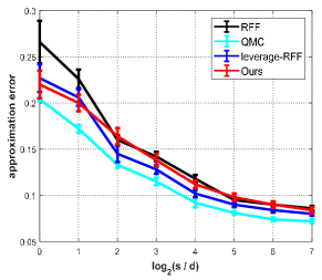
(a) Relative error

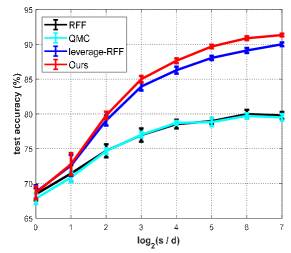
(b) Test accuracy

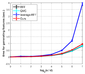
(c) Time cost

Figure 1: Comparison of various algorithms on approximation error in (a), test accuracy in (b), and time cost for generating random features in (c) versus the number of random features $s$ on the EEG dataset.

5 Experiments

In this section, we empirically evaluate the performance of our method equipped with KRR for classification tasks on several benchmark datasets. All experiments are implemented in MATLAB and carried out on a PC with Intel^® i5-6500 CPU (3.20 GHz) and 16 GB RAM. The source code of our implementation can be found in http://www.lfhsgre.org.

5.1 Experimental settings

We choose the popular shift-invariant Gaussian/RBF kernel for experimental validation, i.e., $k(\bm{x},\bm{x}^{\prime})=\exp(-\|\bm{x}-\bm{x}^{\prime}\|^{2}/\sigma^{2})$. Following (?), we use a fixed bandwidth $\sigma=1$ in our experiments. This is without loss of generality since we can rescale the points and adjust the bounding interval. The regularization parameter $\lambda$ is tuned via 5-fold inner cross validation over a grid of $\{0.05,0.1,0.5,1\}$.

Table 2: Dataset statistics.

datasets	#feature dimension	#traing examples	#test examples
EEG	14	7,490	7,490
cod-RNA	8	59,535	157,413
covtype	54	290,506	290,506
magic04	10	9510	9510

Datasets: We consider four classification datasets including EEG, cod-RNA, covtype and magic04; see Tab. 2 for an overview of these datasets. These datasets can be downloaded from https://www.csie.ntu.edu.tw/~cjlin/libsvmtools/datasets/ or the UCI Machine Learning Repository. All datasets are normalized to $[0,1]^{d}$ before the experiments. We use the given training/test partitions on the cod-RNA dataset. For the other three datasets, we randomly pick half of the data for training and the rest for testing. All experiments are repeated 10 times and we report the average classification accuracy as well as the time cost for generating random features.

Compared methods: We compare the proposed surrogate leverage weighted sampling strategy with the following three random features based algorithms:

• RFF (?): The feature mapping $\varphi_{p}(\bm{x})$ is given by Eq. (2), in which the random features $\{\bm{w}_{i}\}_{i=1}^{s}$ are sampled from $p(\bm{w})$.

• QMC (?): The feature mapping $\varphi_{p}(\bm{x})$ is also given by Eq. (2), but the random features $\{\bm{w}_{i}\}_{i=1}^{s}$ are constructed by a deterministic scheme, e.g., a low-discrepancy Halton sequence.

• leverage-RFF (?): The data-dependent random features $\{\bm{w}_{i}\}_{i=1}^{s}$ are sampled from $q^{*}(\bm{w})$. The kernel matrix in $q^{*}(\bm{w})$ is approximated using random features pre-sampled from $p(\bm{w})$.

In our method, we consider sampling from $\tilde{q}^{\prime}(\bm{w})$ in Algorithm 1 for simplicity.

Dataset	$s$	RFF	QMC	leverage-RFF	Ours
		Acc:% (time:sec.)	Acc:% (time:sec.)	Acc:% (time:sec.)	Acc:% (time:sec.)
EEG	$d$	68.45$\pm$0.89 (0.01$\pm$0.00)	67.83$\pm$0.73 (0.02$\pm$0.03)	68.78$\pm$0.97 (0.01$\pm$0.01)	68.62$\pm$0.89 (0.01$\pm$0.00)
	$2d$	71.44$\pm$1.22 (0.02$\pm$0.00)	70.89$\pm$0.72 (0.03$\pm$0.03)	72.59$\pm$1.51 (0.03$\pm$0.01)	72.72$\pm$1.35 (0.02$\pm$0.00)
	$4d$	74.70$\pm$0.94 (0.03$\pm$0.01)	74.66$\pm$0.42 (0.04$\pm$0.03)	79.06$\pm$0.73 (0.05$\pm$0.01)$\bullet$	79.72$\pm$0.58 (0.03$\pm$0.01)$\bullet$
	$8d$	76.96$\pm$0.96 (0.06$\pm$0.02)	77.01$\pm$0.40 (0.07$\pm$0.03)	83.95$\pm$0.58 (0.10$\pm$0.01)$\bullet$	84.97$\pm$0.50 (0.07$\pm$0.02)$\bullet$
	$16d$	78.54$\pm$0.63 (0.11$\pm$0.00)	78.71$\pm$0.29 (0.12$\pm$0.03)	86.29$\pm$0.50 (0.20$\pm$0.01)$\bullet$	87.23$\pm$0.41 (0.13$\pm$0.01)$\bullet$
	$32d$	78.96$\pm$0.44 (0.22$\pm$0.02)	78.83$\pm$0.59 (0.24$\pm$0.06)	88.05$\pm$0.31 (0.49$\pm$0.03)$\bullet$	89.38$\pm$0.32 (0.26$\pm$0.03)$\bullet$
	$64d$	79.97$\pm$0.62 (0.45$\pm$0.01)	79.71$\pm$0.40 (0.47$\pm$0.05)	89.12$\pm$0.36 (1.21$\pm$0.05)$\bullet$	90.36$\pm$0.31 (0.53$\pm$0.02)$\bullet$
	$128d$	79.79$\pm$0.49 (0.82$\pm$0.05)	79.51$\pm$0.47 (0.84$\pm$0.06)	90.01$\pm$0.27 (3.91$\pm$0.09)$\bullet$	91.02$\pm$0.32 (0.96$\pm$0.03)$\bullet$
cod-RNA	$d$	87.02$\pm$0.29 (0.06$\pm$0.01)	87.20$\pm$0.00 (0.07$\pm$0.03)	88.62$\pm$0.92 (0.09$\pm$0.02)	89.64$\pm$0.87 (0.07$\pm$0.01)$\bullet$
	$2d$	87.12$\pm$0.19 (0.12$\pm$0.01)	87.65$\pm$0.00 (0.16$\pm$0.02)	90.42$\pm$1.15 (0.17$\pm$0.01)$\bullet$	90.12$\pm$0.95 (0.13$\pm$0.01)$\bullet$
	$4d$	87.19$\pm$0.08 (0.24$\pm$0.01)	87.44$\pm$0.00 (0.25$\pm$0.02)	92.65$\pm$0.38 (0.35$\pm$0.02)$\bullet$	92.83$\pm$0.33 (0.27$\pm$0.01)$\bullet$
	$8d$	87.27$\pm$0.11 (0.47$\pm$0.02)	87.29$\pm$0.00 (0.49$\pm$0.02)	93.41$\pm$0.07 (0.69$\pm$0.02)$\bullet$	93.49$\pm$0.15 (0.53$\pm$0.02)$\bullet$
	$16d$	87.29$\pm$0.08 (0.91$\pm$0.02)	87.30$\pm$0.00 (0.94$\pm$0.04)	93.71$\pm$0.06 (1.39$\pm$0.05)$\bullet$	93.74$\pm$0.05 (0.99$\pm$0.02)$\bullet$
	$32d$	87.27$\pm$0.05 (1.80$\pm$0.02)	87.33$\pm$0.00 (1.77$\pm$0.01)	93.76$\pm$0.02 (2.82$\pm$0.08)$\bullet$	93.71$\pm$0.07 (1.95$\pm$0.03)$\bullet$
	$64d$	87.30$\pm$0.03 (3.48$\pm$0.15)	87.32$\pm$0.00 (3.54$\pm$0.10)	93.73$\pm$0.03 (6.54$\pm$0.53)$\bullet$	93.99$\pm$0.06 (4.05$\pm$0.08)$\bullet$
	$128d$	87.30$\pm$0.03 (6.79$\pm$0.39)	87.32$\pm$0.00 (6.62$\pm$0.08)	93.66$\pm$0.03 (13.3$\pm$0.23)$\bullet$	93.48$\pm$0.04 (7.78$\pm$0.09)$\bullet$
covtype1	$d$	73.70$\pm$0.79 (1.90$\pm$0.03)	74.71$\pm$0.07 (1.88$\pm$0.11)	73.99$\pm$0.85 (2.96$\pm$0.09)	73.99$\pm$0.63 (2.00$\pm$0.05)
	$2d$	77.09$\pm$0.25 (3.31$\pm$0.21)	77.04$\pm$0.06 (3.37$\pm$0.29)	77.04$\pm$0.35 (5.25$\pm$0.09)	77.02$\pm$0.29 (3.44$\pm$0.10)
	$4d$	79.10$\pm$0.13 (6.27$\pm$0.35)	79.07$\pm$0.07 (6.12$\pm$0.17)	79.18$\pm$0.17 (10.2$\pm$0.15)	79.05$\pm$0.14 (6.58$\pm$0.19)
	$8d$	81.04$\pm$0.12 (12.3$\pm$0.71)	80.90$\pm$0.05 (12.1$\pm$0.45)	81.09$\pm$0.07 (21.1$\pm$0.72)	80.79$\pm$0.11 (13.2$\pm$0.34)
	$16d$	82.42$\pm$0.10 (24.5$\pm$1.02)	82.37$\pm$0.07 (24.3$\pm$1.56)	82.90$\pm$0.12 (46.5$\pm$2.20)	82.18$\pm$0.10 (28.6$\pm$1.58)
magic04	$d$	73.62$\pm$0.68 (0.01$\pm$0.00)	71.74$\pm$0.40 (0.02$\pm$0.04)	73.62$\pm$0.68 (0.01$\pm$0.01)	73.61$\pm$0.68 (0.01$\pm$0.00)
	$2d$	75.89$\pm$0.80 (0.01$\pm$0.01)	75.98$\pm$0.36 (0.03$\pm$0.03)	75.91$\pm$0.77 (0.03$\pm$0.01)	75.88$\pm$0.77 (0.02$\pm$0.00)
	$4d$	77.78$\pm$0.45 (0.03$\pm$0.01)	77.27$\pm$0.33 (0.04$\pm$0.03)	77.78$\pm$0.45 (0.05$\pm$0.01)	77.77$\pm$0.43 (0.03$\pm$0.00)
	$8d$	78.97$\pm$0.34 (0.05$\pm$0.00)	79.07$\pm$0.17 (0.07$\pm$0.03)	79.15$\pm$0.40 (0.09$\pm$0.01)	79.12$\pm$0.34 (0.06$\pm$0.01)
	$16d$	80.04$\pm$0.34 (0.10$\pm$0.01)	79.95$\pm$0.37 (0.11$\pm$0.03)	80.80$\pm$0.40 (0.19$\pm$0.01)	80.74$\pm$0.42 (0.11$\pm$0.01)
	$32d$	80.61$\pm$0.43 (0.19$\pm$0.01)	80.65$\pm$0.31 (0.21$\pm$0.04)	82.00$\pm$0.32 (0.41$\pm$0.03)$\bullet$	82.02$\pm$0.32 (0.22$\pm$0.01)$\bullet$
	$64d$	80.91$\pm$0.28 (0.38$\pm$0.03)	80.85$\pm$0.27 (0.41$\pm$0.05)	82.39$\pm$0.32 (0.93$\pm$0.05)$\bullet$	82.37$\pm$0.25 (0.44$\pm$0.03)$\bullet$
	$128d$	81.10$\pm$0.37 (0.73$\pm$0.03)	81.08$\pm$0.29 (0.76$\pm$0.04)	82.59$\pm$0.29 (2.61$\pm$0.15)$\bullet$	82.55$\pm$0.55 (0.87$\pm$0.02)$\bullet$

• Due to the memory limit, we cannot conduct the experiment on the covtype dataset when $s\geq 32d$.

Table 3: Comparison results of various algorithms for varying $s$ in terms of classification accuracy (mean$\pm$std. deviation %) and time cost for generating random features (mean$\pm$std. deviation sec.). The higher test accuracy means better. Notation “$\bullet$” indicates that leverage-RFF and our method are significantly better than the other two baseline methods via paired t-test.

5.2 Comparison results

High-level comparison:

We compare the empirical performance of the aforementioned random features mapping based algorithms. In Fig. 1, we consider the EEG dataset and plot the relative kernel matrix approximation error, the test classification accuracy and the time cost for generating random features versus different values of $s$. Note that since we cannot compute the kernel matrix $\bm{K}$ on the entire dataset, we randomly sample 1,000 datapoints to construct the feature matrix $\bm{Z}_{s}\bm{Z}_{s}^{\!\top}$, and then calculate the relative approximation error, i.e., $err=\frac{\|\bm{K}-\bm{Z}_{s}\bm{Z}_{s}^{\!\top}\|_{2}}{\|\bm{K}\|_{2}}$.

Fig. 1(a) shows the mean of the approximation errors across 10 trials (with one standard deviation denoted by error bars) under different random features dimensionality. We find that QMC achieves the best approximation performance when compared to RFF, leverage-RFF, and our proposed method. Fig. 1(b) shows the test classification accuracy. We find that as the number of random features increases, leverage-RFF and our method significantly outperform RFF and QMC .

From the above experimental results, we find that, admittedly, QMC achieves lower approximation error to some extent, but it does not translate to better classification performance when compared to leverage-RFF and our method. The reason may be that the original kernel derived by the point-wise distance might not be suitable, and the approximated kernel is not optimal for classification/regression tasks, as discussed in (?; ?; ?). As the ultimate goal of kernel approximation is to achieve better prediction performance, in the sequel we omit the approximation performance of these methods.

In terms of time cost for generating random features, Fig. 1(c) shows that leverage-RFF is quite time-consuming when the total number of random features is large. In contrast, our algorithm achieves comparable computational efficiency with RFF and QMC. These results demonstrate the superiority of our surrogate weighted sampling strategy, which reduces the time cost.

Detailed comparisons:

Tab. 3 reports the detailed classification accuracy and time cost for generating random features of all algorithms on the four datasets. Observe that by using a data-dependent sampling strategy, leverage-RFF and our method achieve better classification accuracy than RFF and QMC on the EEG and cod-RNA dataset when the dimensionality of random features increases. In particular, on the EEG dataset, when $s$ ranges from $2d$ to $128d$, the test accuracy of leverage-RFF and our method is better than RFF and QMC by around 1% to nearly 11%. On the cod-RNA dataset, the performance of RFF and QMC is worse than our method by over 6% when $s\geq 4d$. On the covtype dataset, all four methods achieve similar the classification accuracy. Instead, on the magic04 dataset, our algorithm and leverage-RFF perform better than RFF and QMC on the final classification accuracy if more random features are considered.

In terms of computational efficiency on these four datasets, albeit data-dependent, our method still takes about the similar time cost with the data-independent RFF and QMC for generating random features. Specifically, when compared to leverage-RFF, our method achieves a substantial computational saving.

6 Conclusion

In this work, we have proposed an effective data-dependent sampling strategy for generating fast random features for kernel approximation. Our method can significantly improve the generalization performance while achieving the same time complexity when compared to the standard RFF. Our theoretical results and experimental validation have demonstrated the superiority of our method when compared to other representative random Fourier features based algorithms on several classification benchmark datasets.

References

- [Agrawal et al. 2019] Agrawal, R.; Campbell, T.; Huggins, J.; and Broderick, T. 2019. Data-dependent compression of random features for large-scale kernel approximation. In Proceedings of the 22nd International Conference on Artificial Intelligence and Statistics, 1822–1831.
- [Alaoui and Mahoney 2015] Alaoui, A., and Mahoney, M. W. 2015. Fast randomized kernel ridge regression with statistical guarantees. In Proceedings of Advances in Neural Information Processing Systems, 775–783.
- [Avron et al. 2016] Avron, H.; Sindhwani, V.; Yang, J.; and Mahoney, M. W. 2016. Quasi-Monte Carlo feature maps for shift-invariant kernels. Journal of Machine Learning Research 17(1):4096–4133.
- [Avron et al. 2017] Avron, H.; Kapralov, M.; Musco, C.; Musco, C.; Velingker, A.; and Zandieh, A. 2017. Random Fourier features for kernel ridge regression: Approximation bounds and statistical guarantees. In Proceedings of the 34th International Conference on Machine Learning-Volume 70, 253–262.
- [Bach 2013] Bach, F. 2013. Sharp analysis of low-rank kernel matrix approximations. In Proceedings of Conference on Learning Theory, 185–209.
- [Bach 2017] Bach, F. 2017. On the equivalence between kernel quadrature rules and random feature expansions. Journal of Machine Learning Research 18(1):714–751.
- [Bochner 2005] Bochner, S. 2005. Harmonic Analysis and the Theory of Probability. Courier Corporation.
- [Cohen, Musco, and Musco 2017] Cohen, M. B.; Musco, C.; and Musco, C. 2017. Input sparsity time low-rank approximation via ridge leverage score sampling. In Proceedings of the Twenty-Eighth Annual ACM-SIAM Symposium on Discrete Algorithms, 1758–1777.
- [Cortes, Mohri, and Rostamizadeh 2012] Cortes, C.; Mohri, M.; and Rostamizadeh, A. 2012. Algorithms for learning kernels based on centered alignment. Journal of Machine Learning Research 13(2):795–828.
- [Dao, De Sa, and Ré 2017] Dao, T.; De Sa, C. M.; and Ré, C. 2017. Gaussian quadrature for kernel features. In Proceedings of Advances in neural information processing systems, 6107–6117.
- [Evans 1993] Evans, G. 1993. Practical numerical integration. Wiley New York.
- [Fanuel, Schreurs, and Suykens 2019] Fanuel, M.; Schreurs, J.; and Suykens, J.A.K. 2019. Nyström landmark sampling and regularized Christoffel functions. arXiv preprint arXiv:1905.12346.
- [Gauthier and Suykens 2018] Gauthier, B., and Suykens, J.A.K. 2018. Optimal quadrature-sparsification for integral operator approximation. SIAM Journal on Scientific Computing 40(5):A3636–A3674.
- [Li et al. 2019] Li, Z.; Ton, J.-F.; Oglic, D.; and Sejdinovic, D. 2019. Towards a unified analysis of random Fourier features. In Proceedings of the 36th International Conference on Machine Learning, 3905–3914.
- [Mall and Suykens 2015] Mall, R., and Suykens, J.A.K. 2015. Very sparse LSSVM reductions for large-scale data. IEEE Transactions on Neural Networks and Learning Systems 26(5):1086–1097.
- [Munkhoeva et al. 2018] Munkhoeva, M.; Kapushev, Y.; Burnaev, E.; and Oseledets, I. 2018. Quadrature-based features for kernel approximation. In Proceedings of Advances in Neural Information Processing Systems, 9165–9174.
- [Niederreiter 1992] Niederreiter, H. 1992. Random number generation and quasi-Monte Carlo methods, volume 63. SIAM.
- [Rahimi and Recht 2007] Rahimi, A., and Recht, B. 2007. Random features for large-scale kernel machines. In Proceedings of Advances in Neural Information Processing Systems, 1177–1184.
- [Rudi, Camoriano, and Rosasco 2017] Rudi, A.; Camoriano, R.; and Rosasco, L. 2017. Generalization properties of learning with random features. In Proceedings of Advances in Neural Information Processing Systems, 3215–3225.
- [Schölkopf and Smola 2003] Schölkopf, B., and Smola, A. J. 2003. Learning with kernels: support vector machines, regularization, optimization, and beyond. MIT Press.
- [Sinha and Duchi 2016] Sinha, A., and Duchi, J. C. 2016. Learning kernels with random features. In Proceedins of Advances in Neural Information Processing Systems. 1298–1306.
- [Sun, Gilbert, and Tewari 2018] Sun, Y.; Gilbert, A.; and Tewari, A. 2018. But how does it work in theory? Linear SVM with random features. In Proceedings of Advances in Neural Information Processing Systems, 3383–3392.
- [Suykens et al. 2002] Suykens, J.A.K.; Van Gestel, T.; De Brabanter, J.; De Moor, B.; and Vandewalle, J. 2002. Least Squares Support Vector Machines. World Scientific.
- [Tropp and others 2015] Tropp, J. A., et al. 2015. An introduction to matrix concentration inequalities. Foundations and Trends® in Machine Learning 8(1-2):1–230.
- [Yu et al. 2016] Yu, F. X.; Suresh, A. T.; Choromanski, K.; Holtmannrice, D.; and Kumar, S. 2016. Orthogonal random features. In Proceedings of Advances in Neural Information Processing Systems, 1975–1983.
- [Zhang et al. 2019] Zhang, J.; May, A.; Dao, T.; and Re, C. 2019. Low-precision random fourier features for memory-constrained kernel approximation. In Proceedings of the 22nd International Conference on Artificial Intelligence and Statistics, 1264–1274.