Gradient-based Optimization for Bayesian Preference Elicitation
Abstract
Effective techniques for eliciting user preferences have taken on added importance as recommender systems (RSs) become increasingly interactive and conversational. A common and conceptually appealing Bayesian criterion for selecting queries is expected value of information (EVOI). Unfortunately, it is computationally prohibitive to construct queries with maximum EVOI in RSs with large item spaces. We tackle this issue by introducing a continuous formulation of EVOI as a differentiable network that can be optimized using gradient methods available in modern machine learning (ML) computational frameworks (e.g., TensorFlow, PyTorch). We exploit this to develop a novel, scalable Monte Carlo method for EVOI optimization, which is more scalable for large item spaces than methods requiring explicit enumeration of items. While we emphasize the use of this approach for pairwise (or -wise) comparisons of items, we also demonstrate how our method can be adapted to queries involving subsets of item attributes or “partial items,” which are often more cognitively manageable for users. Experiments show that our gradient-based EVOI technique achieves state-of-the-art performance across several domains while scaling to large item spaces.
1 Introduction
Rapid advances in AI, machine learning, speech and language technologies have enabled recommender systems (RSs) to become more conversational and interactive. Increasingly, users engage RSs using language-based (speech or text) and multi-modal interfaces that have the potential to increase communication bandwidth with users compared to passive systems that make recommendations based only on user-initiated engagement. In such contexts, actively eliciting a user’s preferences with a limited amount of interaction can be critical to the user experience.
Preference elicitation has been widely studied in decision analysis and AI (?; ?; ?; ?), but has received somewhat less attention in the recommender community (we discuss exceptions below). Bayesian methods have proven to be conceptually appealing for elicitation; in particular, expected value of information (EVOI) offers a principled criterion for selecting preference queries and determining when to make recommendations. EVOI is relatively practical in domains with small decision spaces and, as such, can be applied to certain types of content-based RSs, e.g., those with small “catalogs” of attribute-based items. However, maximizing EVOI is generally computationally intractable and often unable to scale to realistic settings with millions of items.
Our work aims to make Bayesian elicitation more practical. Our first contribution is a novel formulation of the problem of selecting a slate query with maximum EVOI as a continuous optimization in a differentiable network. This allows the problem to be solved using gradient-based techniques available in modern ML computational frameworks such as TensorFlow or PyTorch. The key to our approach is relaxing the set of items from which recommendations and queries are generated by allowing attributes to vary continuously without requiring they correspond to available items (these could be interpreted as “hypothetical” items in attribute- or embedding-space). Once optimized in this relaxed fashion, any hypotheticals are projected back into the nearest actual items to generate suitable recommendations or queries. We also propose regularizers that can be used during optimization to keep hypothetical items close to some actual item. We show empirically that this approach achieves comparable performance to state-of-the-art discrete methods, and also offers several key advantages: (a) it leverages highly optimized ML software and hardware for ease of implementation, performance and parallelization; (b) it generalizes to a variety of query types, including those involving items not present in the dataset, or partially specified items; (c) it accommodates continuous item attributes; and (d) it can use arbitrary differentiable metrics and non-linear utilities, allowing end-to-end optimization using gradient ascent.
Our second contribution leverages this flexibility—we propose a novel elicitation strategy based on partial comparison queries. In multi-attribute domains where items have large numbers of attributes, asking a user to compare complete items can be impractical (e.g., with voice interfaces) or cognitively burdensome. Instead we ask the user to compare partially instantiated items, with only a small number of attributes specified as is common in decision analysis (?). Finding EVOI-optimal partial queries is a difficult combinatorial problem, but we develop a simple, efficient continuous optimization method using the ideas above that performs well in practice.
The remainder of the paper is organized as follows. We outline related work in Sec. 2. In Sec. 3 we lay out the framework and preliminary concepts upon which our contributions are based, including: Bayesian recommendation, recommendation slates, EVOI, preference elicitation, and several existing computational approximations used for Bayesian elicitation, including the query iteration algorithm (?). We introduce our basic continuous relaxation for Bayesian recommendation and EVOI computation using choice or comparison queries involving fully specified items in Sec. 4, and several algorithmic variants based on it. In Sec. 5 we apply the same principles to elicitation using queries that use only subsets of attributes. We provide detailed empirical evaluation of our methods in Sec. 6, analyzing both recommendation quality as a function of number of queries, and the computational effectiveness of our methods. We conclude with brief remarks on future research directions in Sec. 7.
2 Related Work
Preference elicitation has long been used to assess decision-maker preferences in decision analysis (?; ?; ?), marketing science (?) and AI (?; ?), often exploiting the multi-attribute nature of actions/decisions. In RSs, elicitation has primarily been studied in domains where items have explicit attributes and the recommendable space has a relatively small numbers of items (e.g., content-based as opposed to collaborative filtering (CF) RSs), which makes such settings qualitatively similar to other multi-attribute settings (?).
Most work on elicitation assumes some uncertainty representation over user preferences or utility functions, some criterion for making recommendations under such uncertainty, and uses one or more types of query to reduce that uncertainty. A variety of work uses strict uncertainty in which (the parameters of) a user’s utility function are assumed to lie in some region (e.g., polytope) and queries are used to refine this region. Various decision criteria can be used to make recommendations in such models (e.g., using a centroid (?)), with minimax regret being one popular criterion in the AI literature (?). Queries can be selected based on their ability to reduce the volume or surface of a polytope, to reduce minimax regret, or other heuristic means.
A variety of query types can be used to elicit user preferences. It is common in multi-attribute utility models to exploit utility function structure to ask users about their preferences for small subsets of attributes (?; ?; ?). Techniques based on multi-attribute utility theory—the focus of our work—have been applied to RSs (see Chen & Pu (?) for an overview). For example, critiquing methods (?; ?) present candidate items to a user, who critiques particular attributes (e.g., “I’d prefer a smaller item”) to drive the next recommendations toward a preferred point, while unconstrained natural language conversations offer further flexibility (?). We focus on elicitation methods that use set-wise/slate choice queries: a user is presented with a slate of (often multi-attribute) items and asked to state which is their most preferred. If , this is a classic pairwise comparison. Such queries are common in decision support, conjoint analysis and related areas.
In this work, we focus on Bayesian elicitation, in which a distribution over user utility functions (or parameters) is maintained and updated given user responses to queries. A fully Bayesian approach requires one to make recommendations using expected utility w.r.t. this distribution (?; ?; ?), but other criteria can be used for reasons of computational efficiency, e.g., minimizing maximum expected regret (loss) of a recommendation w.r.t. the utility distribution (?).
Expected value of information (EVOI) (?) provides a principled technique for elicitation in Bayesian settings. EVOI requires that one ask queries such that posterior decision (or recommendation) quality (i.e., user utility) is maximized in expectation (w.r.t. to possible user responses). Such queries are, by construction, directly relevant to the decision task at hand. In RSs, “value” is usually defined as the utility of the top recommended item. Guo and Sanner (?) select high EVOI queries assuming a diagonal Gaussian distribution over user utilities, but their algorithms evaluate all pairwise queries (or in their “greedy” algorithm), neither of which are practical for real-time elicitation over millions of items. The most direct predecessor of our work is that of Viappiani and Boutilier (?), who propose an approximate iterative algorithm for EVOI optimization that only considers a small number of queries. We provide details of this approach in Sec. 3.4.
Other approaches to elicitation using distributions over user preferences include various forms of maximum information gain. These ask the query whose expected response offers maximal information according to some measure. Canal et al. (?) select pairwise comparisons by maximizing mutual information between the user response and the user preference point in some high-dimensional space. Rokach et al. (?) select the pairwise query that minimizes “weighted generalized variance,” a measure of posterior spread once the query is answered, while Zhao et al. (?) ask the “least certain” pairwise comparison constructed from the top items (or between the top and the rest). While often more tractable than EVOI, information gain criteria suffer (compared to EVOI) from the fact that not all information has the same influence on recommendation quality—often only a small amount of information is decision-relevant. Other non-Bayesian query selection criteria are possible; e.g., Bourdache et al. (?) use a variant of the current solution strategy (?) for generating pairwise comparison queries.
The continuous optimization method we propose in this work can handle arbitrary combinatorial items with both discrete and continuous attributes. Such a setting is studied in (?), where point estimates of utility are used, with a structured perceptron-like update after each query. Dragone et al. (?) use partially specified items for elicitation, but consider a critiquing model of interaction whereas we focus on set-wise comparisons.
While content-based RSs model user preferences w.r.t. item attributes, in large, commercial RSs user preferences are usually estimated using user interaction data collected passively. Preferences are modeled using CF (?; ?), neural CF (?)) or related models, which often construct their own representations of items, e.g., by embedding items in some latent space. Among the earliest approaches to elicitation with latent item embeddings are active CF techniques (?; ?) that explicitly query users for item ratings; more recently Canal et al. (?) similarly elicit over item embeddings. In this work, we also generate comparison queries using learned item embeddings, though our methods apply equally to observable item attributes.
Finally, we note that elicitation has strong connections to work on Bayesian (or blackbox) optimization (?), where the aim is to find the optimum of some function—analogous to finding a good recommendation for a user—while minimizing the number of (expensive) function evaluations—analogous to minimizing the number/cost of user queries. In contrast with most work in preference elicitation, Bayesian optimization methods typically focus on direct function evaluation, equivalent to asking a user for their utility for an item, as opposed to asking for a qualitative comparisons, though recent work considers dueling bandit models using pairwise comparisons in Bayesian optimization (?; ?). Such techniques are generally derivative-free, though recent work considers augmenting the search for an optimum with (say, sampled) gradient information (e.g., (?)). We use gradient information when computing EVOI, directly exploiting the linear nature of user utility in embedding space.
3 Background
We begin by outlining the basic framework, notation, and prior results on which our methods are based.
3.1 Bayesian Recommendation
We adopt a Bayesian approach to recommendation and elicitation in which the RS maintains a probabilistic belief about a user’s utility function over recommendable items. It uses this to generate both recommendations and elicitation queries. A recommendation problem has six main components: an item set, a user utility function drawn from a utility space, a prior belief over utility space, a query space, a response space, and a response model. We outline each in turn.
We assume a set of recommendable items , each an instantiation of (for ease of exposition, real-valued) attributes (categorical attributes can be converted in standard fashion). These attributes may be dimensions in some latent space, say, as generated by some neural CF model (see Sec. 6.) A user, for whom a recommendation is to be made, has a linear utility function over items, parameterized as a vector , where ; i.e., for any .111Linearity of utility may be restrictive if the attributes are observable or “catalog” properties of items as opposed to reflecting some learned embedding. Our methods can be extended to other utility representations in such a case, for example, UCP- (?) or GAI-networks (?; ?), which offer a linear parameterization of utility functions without imposing linearity w.r.t. the attributes themselves. A user’s most preferred item is that with greatest utility: The regret of any recommendation is and is a natural measure of recommendation quality. Finally, we assume the RS has some prior belief over . This reflects its uncertainty over the true utility function of the user.
The prior is typically derived from past interactions with other users, and reflects the heterogeneity of user preferences in the domain. While we explicate our techniques in the cold-start regime where the RS has no information about the user in question, may also incorporate past interactions or other information about that user—this has no impact on our methodology. The prior will be updated as the RS interacts with the user, and we use generically to denote the RS’s current belief.
Given a belief , the expected utility of an item (or recommendation) is:
| (1) |
The optimal recommendation given is the item with maximum expected utility:
| (2) |
The RS can refine its belief and improve recommendation quality by asking the user questions about her preferences. Let be the query space. For any query , the response space reflects possible user responses to . For example, a pairwise comparison query (e.g., “do you prefer to ?”) has a binary response space (yes, no). For any sequence of queries , , to simplify notation we assume that any corresponding sequence of user responses , where , uniquely determines (e.g., through suitable relabeling so that a “yes” response to some is encoded differently than a “yes” to a different ). We also assume the RS has a response model that specifies the probability of a user with utility function offering response when asked query .
We focus on slate (comparison) queries, , , in which a slate of items is presented to the user, who is asked which is most preferred.222The response set can be augmented with a “null” item to account for, say, a “none of the above” response. We consider two response models for slate queries. The noiseless response model assumes a user responds with the utility maximizing item: . The logistic response model assumes , where temperature controls the degree of stochasticity/noise in the user’s choice. Other choice models could be adopted as well (?).
We assume the response to any query is conditionally independent of any other given . Let be the expected probability of response given belief . Given any response sequence (which determines the generating query sequence ) and current belief , the posterior belief of the RS is given by Bayes rule:
3.2 Expected Value of Information
While computing optimal query strategies can be cast as a sequential decision problem or POMDP (?; ?), we adopt a simpler, commonly used approach, namely, myopic selection of queries using the well-founded expected value of information (EVOI) criterion (?; ?). Given belief , we first define the expected utility (w.r.t. possible responses) of the best recommendation after the user answers query :
Definition 1.
The posterior expected utility (PEU) of is:
| (3) |
The (myopic) expected value of information is .
A query with maximum PEU maximizes the expected utility of the best recommendation conditioned on the user’s response. EVOI, which is maximized by the same query, measures the improvement in expected utility offered by the query relative to the prior belief and can serve as a useful metric for terminating elicitation.
3.3 EVOI Optimization with Particle Filtering
We use a Monte Carlo approach to optimize EVOI as in (?). Given belief , we sample points from and maximize the sample average to approximate the integral within EVOI:
For slate queries under logistic response, an optimal query w.r.t. EVOI satisfies:
| (4) |
Computing EVOI for a single query using this approach requires time. Consequently, search over all queries to maximize EVOI is prohibitively expensive, even in the pairwise case (), when is moderately large.
3.4 Query Iteration
While finding optimal EVOI queries is intractable, effective heuristics are available. Notice that computing EVOI for a query requires identifying the items with greatest posterior expected utility conditioned on each potential user response , i.e., the maximizing items in Eq. 4. We refer to this operation as a deep retrieval for query , and write . We sometimes refer to as the query slate and as the (posterior) recommendation slate.
The following result tells us that replacing the query slate with the induced recommendation slate increases EVOI:
Theorem 2 (? ?).
Let be a slate query with . Under noiseless response, ; while under logistic response, , where
This suggests a natural iterative algorithm : start with a query slate, replace it with its induced recommendation slate, repeat until convergence. Viappiani and Boutilier (?) find that, in practice, converges quickly and finds high EVOI queries in settings with small item sets.
4 Continuous EVOI Optimization
While is often an effective heuristic, it cannot scale to settings with large item spaces: each iteration requires the computation of the item with maximum PEU for each of the responses; but computing this maximum generally requires EU computation for each candidate item.
To overcome this, we develop a continuous optimization formulation for EVOI maximization. Intuitively, we “relax” the discrete item space to obviate the need for enumeration, and treat the items in the query and recommendation slates as continuous vectors in . Once EVOI is optimized in the relaxed problem using gradient ascent, we project the solution back into the discrete space to obtain a slate query using only feasible items. Apart from scalability, this offers several advantages: we can exploit highly optimized and parallelizable ML frameworks (e.g. TensorFlow) and hardware for ease of implementation and performance; variants of our methods described below have common, reusable computational elements; and the methods are easily adapted to continuous item spaces and novel query types (see Sec. 5.)
4.1 A Reference Algorithm
We develop a basic continuous formulation by considering the EVOI objective in Eq. 4—we focus on logistic response for concreteness. In the discrete case, each item (in the query slate) and (recommendation slate) are optimized by enumerating the feasible item set . We relax the requirement that items lie in and treat these as continuous variables. Let (query slate) and (recommendation slate) be two matrices whose -th columns represent and , respectively. Let be an matrix whose rows are the sampled utilities . We can express the softmax probabilities in the inner sum of Eq. 4 as , constructing a row vector of probabilities (each element is a logit).
Similarly, the dot products in the outer sum can be expressed as . The Hadamard (element-wise) product gives:
Summing over and averaging over , we obtain:
| (5) |
where is a -vector of 1s. If we maximize for any given , this is exactly the PEU of query slate . We can then apply gradient-based methods to optimize (to compute PEU) and (to find the best query) as we detail below.
A solution may contain infeasible items depending on the optimization method used, in which case we must project the query slate into item space —we discuss mechanisms for this below. One approach is to leverage Thm. 2, and perform one deep retrieval to select feasible (optimal) recommendation items given . Thm. 2 ensures that , interpreted as a query, is a better feasible slate (or at least not much worse) than . To avoid duplicate ’s, we deep retrieve the top- items for each possible user response and only add distinct items to the query slate (see Alg. 1). Alg. 2 details this basic “reference” algorithm. We now discuss variations of the reference algorithm.

4.2 Taxonomy of Continuous EVOI Algorithms
The reference algorithm can be instantiated in different ways, depending on how we represent the (continuous) query and recommendation slates and , and how we project these into feasible item space. These three choices form a taxonomy of continuous EVOI algorithms:
Query Slate Representation
. The simplest way to represent queries are as “unconstrained” variables uninfluenced by the feasible set (though possibly with some norm constraint). However, in most applications feasible items will be sparsely distributed in and such unconstrained optimization may yield queries far from any feasible item. To address this, we can incorporate “soft” feasibility constraints as regularization terms in the optimization, encouraging each to be near some feasible item. We note that this restriction can magnify local optimality issues.
Recommendation Slate Representation
. As above, we can also treat the recommendation slate items as unconstrained variables or regularize them to be near feasible items. We consider two other approaches, allowing a tradeoff between computational ease and fidelity of EVOI computation. The first equates the query and recommendation slates. Thm. 2 implies that there exist optimal EVOI queries where the two coincide, i.e. , under noiseless response, and do so approximately under logistic response. Using a single set of slate variables in Eq. 5 for both gives the following optimization:
| (6) |
A more computationally expensive, but more accurate, approach for EVOI avoids relaxing the query slate, instead computing exact EVOI for . This requires deep retrieval operations (one per item) over at each optimization step. In practice, we can apply deep retrieval only periodically, giving an alternating optimization procedure that optimizes query variables given the recommendation slate at one stage and deep retrieving the recommendation items given the query variables the next. One could also compute the max over a small subset of prototype items.
Projecting to Feasible Items
. The (query) values after optimization will not generally represent feasible items. We could recover a feasible query by projecting each to its nearest neighbour in , but this might give poor queries, e.g., by projecting an informative infeasible pairwise comparison to two feasible items that differ in only a dimension that offers no useful information. Instead, we use a single deep retrieval of to obtain a set of to serve as the query.
4.3 Variants of Continuous EVOI Algorithms
We identify four natural algorithms motivated by the taxonomy above. The modularity of our approach allows the design of a single network architecture, shown in Fig. 1, that supports all of these algorithms due to its reusable elements. See Appendix A.2 for additional details.
-
•
. Equate query and recommendation slates; unconstrained except for an norm bound on variables.
-
•
. Like but with an added regularization ensuring the variables stay close to feasible items.
-
•
. Query variables are unconstrained, deep retrieval occurs at every optimization step.
-
•
. Query variables are unconstrained, and we use the alternating optimization described above.
All four algorithms use one deep retrieval at completion to ensure the resulting slate query uses feasible items in .
4.4 Initialization Strategies
Since the optimization objective is non-convex, we can (and do, in practice) encounter multiple local optima in each algorithm variant. Hence, the initialization strategy can impact results, so we consider several possibilities. The first strategy, , initializes the optimization with random vectors. The second follows (?), initializing the slate query with the highest-utility items for randomly selected utility particles (which they find performs well in conjunction with ). We call this strategy . A third strategy, , initializes using a query slate that splits the sampled utility particles into evenly weighted groups in which each of the responses results in roughly utility particles that are (mostly) consistent with the response. Such balanced queries may use infeasible items. In practice, we use multiple restarts to mitigate the effects of local maxima.
5 Partial Comparison Queries
In many domains, slate queries with fully specified items are impractical: they can impose a significant cognitive burden on the user (e.g., comparing two car configurations with dozens of attributes); and often a user lacks the information to determine a preference for specific items (e.g. comparing two movies the user has not seen). It is often more natural to use partial comparison queries with items partially specified using a small subset of attributes (e.g., truck vs. coupe, comedy vs. drama). Finding partial queries with good EVOI requires searching through the combinatorial space of queries (attribute subsets). Unlike full queries, with partial queries the query and item spaces are distinct. However, we can readily adapt our continuous EVOI methods.
5.1 Semantics of Partial Comparisons
The most compelling semantics for partial comparisons may generally be domain specific, but in this work we adopt the simple ceteris paribus (all else equal) semantics (?). Let be defined over attributes . Given , a partial item is a vector with values defined over attributes in . We assume there is some s.t. (i.e., any partial item has a feasible completion). Given partial query slate , a uniform completion of is any full query such that (i.e., each item is completed using the same values of attributes ). Ceteris paribus responses require that, for any uniform completion of :
This condition holds under, say, additive independence (?) and induces an especially simple response model if we assume utilities are linear. For instance, with logistic responses, we have:
Thus our response model for partial queries is similar to those for full queries. The optimal EVOI problem must find both attributes and partial items:
5.2 Continuous EVOI for Partial Comparisons
As in Sec. 4, we need a continuous slate representation and projection method. For query representation, we relax partial items to fall outside . W.l.o.g., let attribute values be binary with a relaxation in and a partial item vector be a point in . Rather than representing the recommendation slate explicitly, we compute exact EVOI at each step of optimization (deep retrieval). We project to partial queries by only specifying a small number of attributes for each item: we discretize by setting the highest attribute values for each item to and the rest to . This projection could cause arbitrary loss in EVOI, so we use -regularization to encourage each to have values close to and the rest close to . The optimization objective becomes:
| (7) |
where sorts elements of a vector in ascending order, is a -dimensional vector with the last coordinates set to and the rest to , and is the regularization constant. We call this the algorithm.
6 Experiments
We assess our continuous EVOI algorithms by comparing their speed and the quality of queries they generate to several baseline methods in two sets of experiments: the first uses full-item comparison queries, the second uses our partial comparison queries. We are primarily interested in comparing elicitation performance using (true) regret over complete elicitation runs—in a real scenario, one would generally evaluate the quality of recommendations after each round of elicitation. Since all methods attempt to maximize EVOI, we also report EVOI.
In all experiments, we sample utility vectors from some prior to serve as “true users”, and simulate their query responses assuming a logistic response model. Regret is the difference in (true) utility of the best item under and that of the item with greatest EU item given the posterior. Further experimental details (e.g., on utility priors, gradient optimization configurations, data sets) can be found in Appendix A.3. To reduce the effect of local EVOI maxima, we run our continuous methods and with initialization restarts (unless otherwise stated) using one of random, or initializers.
6.1 Slate Comparisons with Complete Items
For full-item slates, we compare to the following baselines:
-
: Queries composed of randomly selected items.
-
: Exhaustive search for the best slate among the top EU items.
-
: The greedy algorithm of Viappiani and Boutilier (?), which incrementally appends to the query slate the item that maximizes slate utility (given items already on the slate).
-
: The iterative algorithm from Sec. 3.4.
-
: The “sampling initialization” heuristic of Viappiani and Boutilier (?), which uses the item with greatest utility for each of randomly selected utility particles (which we find performs well on its own).
-
: Exhaustive search (over all queries) for an optimal EVOI query.
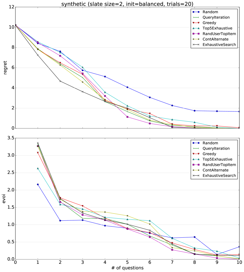
Synthetic
. We consider a synthetic dataset where we sample both items and utility particles with dimension from . We run 20 trials of simulated elicitation, each sampling items and utility vectors. Results are plotted for pairwise comparisons in Fig. 2 (averaged regret is an empirical estimate of “expected loss” as defined by Chajewska et al. (?)). Of the continuous methods, only is plotted to reduce clutter in the figure. We first consider regret. The initial regret is (no queries); and to reach regret of , takes queries (other continuous methods perform similarly) while , and require queries. EVOI performance mirrors that of regret. Note that the EVOI of different methods is not generally comparable after the first query, since different queries result in different posteriors. The best performing strategies for the first query (EVOI) are (), (), (), and (). performs worst with EVOI . Overall, these methods are competitive with , which achieves an average EVOI of on the first query. In terms of regret, is quite competitive: achieving among the least regret across the first four queries. Because is myopic, it achieves the lowest regret only for the first few queries.
| MovieLens | Goodreads | |||||
|---|---|---|---|---|---|---|
| , , | , , | , , | , , | , , | , , | |
| 0.01 (0.00) | 0.04 (0.00) | 0.14 (0.00) | 0.77 (0.08) | 4.26 (0.29) | 17.62 (0.52) | |
| 2.56 (0.17) | 2.71 (0.09) | 2.24 (0.06) | 2.54 (0.06) | 2.96 (0.06) | 3.14 (0.06) | |
| 0.88 (0.04) | 0.95 (0.05) | 0.78 (0.04) | 0.85 (0.04) | 0.94 (0.04) | 1.00 (0.04) | |
| 1+ day | N/A | N/A | N/A | N/A | N/A | |
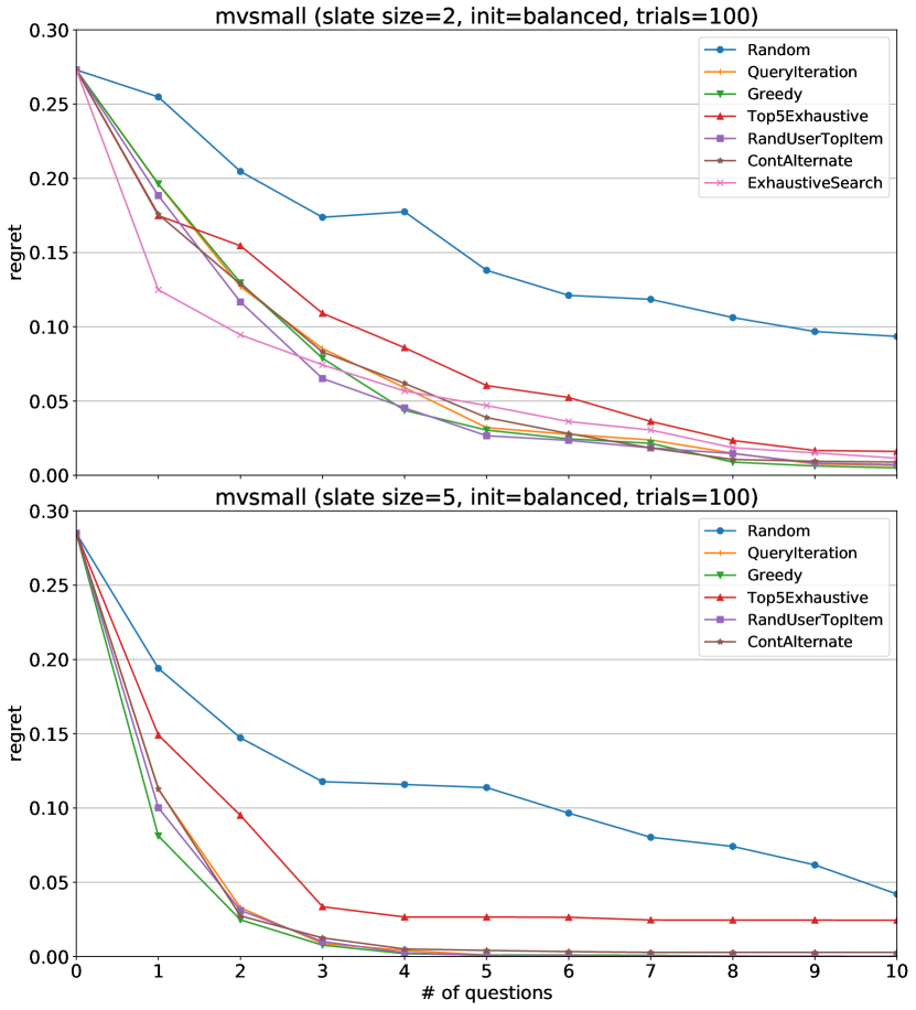
MovieLens
. Using the MovieLens 100-K dataset, we train user and movie embeddings with dimension . Regret plots are shown in Fig. 3 for slate sizes and , averaged over elicitation trials of queries (using items and random selections of user embeddings in each trial). Again, is the only continuous method plotted to reduce clutter. Regret starts at slightly below . For pairwise comparisons, takes queries to reduce regret to ( of the original regret) while (best continuous method), , and each require queries. Interestingly, while reduces regret the most with the first two queries, it does not sustain its performance over a longer trajectory, likely due its myopic objective. While performs best on the first query (both w.r.t. regret and EVOI) it does not maintain the same regret performance (or high EVOI) in subsequent rounds and requires queries to reach regret . This demonstrates one weakness of myopic EVOI and the importance of non-myopic elicitation. For slates of size of , as expected, the same top methods require about half as many queries ( to ) to reduce regret to the same point (). In terms of EVOI on the first query, for pairwise comparisons, the (in general, intractable) method performs best with EVOI of , while and are nearly as good, with and , respectively. Next best is with , and the remaining methods achieve or below. For slate size , performs best with , followed by and with . , and are also competitive with EVOI from ; meanwhile performs weaker with (and is worse on all trials vs. all other methods).
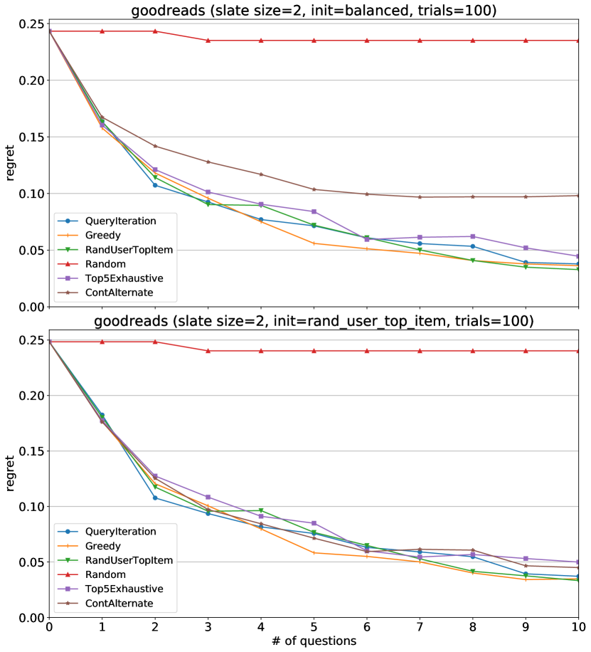
Goodreads
. The last experiments use the much larger Goodreads dataset. We train a user and item embedding model. Each trial consists of a random set of items (books) and a random set of user embeddings. Due to the large item space, we did not run and (it is possible to run them on subsampled item sets). Using initialization, the regret profile of continuous methods is not as competitive as above; e.g., in Fig. 4 we see it reaches regret after queries. Random performs significantly worse with this large item space. This is likely because most item pairs are not significantly different or the user embeddings tend not to vary much. If we instead use to initialize (as does), we obtain competitive results w.r.t. both regret and EVOI. We suspect that there could be significant structure in the (high-dimensional) item space that volumetric initialization does not capture well, resulting in poor local maxima. The choice of initialization has a similar impact on the EVOI of the first query. Our continuous methods achieve EVOI of about compared to for other methods.
Wall clock runtimes
. We benchmark the algorithmic runtimes on a workstation with a 12-core Intel Xeon E5-1650 CPU at 3.6GHz, and 64GB of RAM. We measure the performance of , , and (with initialization) since the other algorithms that are competitive in terms of EVOI are not computationally scalable. Results are shown in Table 1. We run 10 trials with 10 queries per trial for each algorithm and under each parameter setting. Note that is simply not scalable beyond the smallest problem instances. We implement using primarily matrix operations. For relatively small problems is fast, requiring at most s for MovieLens and Goodreads (where the number of items, ). However, and as expected, scaling is an issue for as it takes s to solve for pairwise comparisons with items and particles/users. For a larger slate size of on Goodreads, becomes even less practical, requiring s to generate a query. Continuous methods scale better, with taking only s on the largest problem instance while is even faster, taking at most s to generate a query (and is more consistent over all problem sizes)
6.2 Slate Comparisons with Partial Items
For partial comparison queries, we assess the quality of queries found by by comparing the EVOI of the cold-start query it finds vìs-a-vìs three natural reference algorithms: (1) random queries; (2) a natural extension of for the partial setting—start with the attribute having highest utility variance across users, then greedily add attributes that result in the highest EVOI; and (3) exhaustive search for the best EVOI query.
We use the MovieLens-20M (?) dataset and represent each movie with binary attributes from the Tag Genome (?). We evaluate EVOI on the first query by randomly selecting user embeddings as the prior, and running for 100 restarts. We initialize query embeddings to random uniform values in , then run gradient ascent on Eq. 7 for 100 steps, initializing the regularization weight at and multiplying by each iteration.
7 Conclusion and Future Work
We have developed a continuous relaxation for EVOI optimization for Bayesian preference elicitation in RSs that allows scalable, flexible gradient-based approaches. We also leveraged this approach to develop an EVOI-based algorithm for partial comparison queries. Our methods readily handle domains with large item spaces, continuous item attributes, and can be adapted to other differentiable metrics. They can also leverage modern ML frameworks to exploit various algorithmic, software and hardware efficiencies. Our experiments show that continuous EVOI achieves state-of-the-art results in some domains.
There are various avenues for future work. Further exploration of different forms of partial comparisons is of interest, including the use of latent or high-level conceptual features while using continuous elicitation methods to generate informative queries from a much larger, perhaps continuous, query space. Methods that incorporate user knowledge, natural language modeling and visual features, together with explicit or latent attributes during elicitation would be of great value. Finally, evaluating recommendations using traditional ranking metrics and conducting user studies will play a key role in making elicitation more user-friendly.
References
- [Bourdache, Perny, Spanjaard 2019] Bourdache, N.; Perny, P.; and Spanjaard, O. 2019. Incremental elicitation of rank-dependent aggregation functions based on Bayesian linear regression. IJCAI-19, 2023–2029.
- [Boutilier, Bacchus, and Brafman 2001] Boutilier, C.; Bacchus, F.; and Brafman, R. I. 2001. UCP-Networks: A directed graphical representation of conditional utilities. UAI-01, 56–64.
- [Boutilier et al. 2006] Boutilier, C.; Patrascu, R.; Poupart, P.; Schuurmans, D. 2006. Constraint-based optimization and utility elicitation using the minimax decision criterion. Art. Int. 170:686–713.
- [Boutilier, Zemel, and Marlin 2003] Boutilier, C.; Zemel, R. S.; and Marlin, B. 2003. Active collaborative filtering. UAI-03, 98–106.
- [Boutilier 2002] Boutilier, C. 2002. A POMDP formulation of preference elicitation problems. AAAI-02, 239–246.
- [Braziunas and Boutilier 2005] Braziunas, D., and Boutilier, C. 2005. Local utility elicitation in GAI models. UAI-05, 42–49.
- [Burke 2002] Burke, R. 2002. Interactive critiquing for catalog navigation in e-commerce. Art. Int. Rev. 18:245–267.
- [Canal et al. 2019] Canal, G.; Massimino, A.; Davenport, M.; and Rozell, C. 2019. Active embedding search via noisy paired comparisons. ICML-19.
- [Chajewska, Koller, and Parr 2000] Chajewska, U.; Koller, D.; Parr, R. 2000. Making rational decisions using adaptive utility elicitation. AAAI-00, 363–369.
- [Chen and Pu 2004] Chen, L., and Pu, P. 2004. Survey of preference elicitation methods. Technical Report TR IC/2004/67, EPFL.
- [Dragone et al. 2018] Dragone, P.; Teso, S.; Kumar, M.; and Passerini, A. 2018. Decomposition strategies for constructive preference elicitation. AAAI-18.
- [Dragone, Teso, and Passerini 2017] Dragone, P.; Teso, S.; and Passerini, A. 2017. Constructive preference elicitation over hybrid combinatorial spaces. CoRR abs/1711.07875.
- [Fishburn 1967] Fishburn, P. 1967. Interdependence and additivity in multivariate, unidimensional expected utility theory. International Economic Review 8:335–342.
- [Fishburn 1977] Fishburn, P. C. 1977. Multiattribute utilities in expected utility theory. In Bell, D. E.; Keeney, R. L.; and Raiffa, H., eds., Conflicting Objective in Decisions. Wiley. 172–196.
- [Fu 2016] Fu, H. 2016. Python implementation of probabilistic matrix factorization algorithm for building a recommendation system using MovieLens ml-100k. Accessed: 2019-08-31.
- [Gonzales and Perny 2004] Gonzales, C., and Perny, P. 2004. GAI networks for utility elicitation. (KR-04), 224–234.
- [González et al. 2017] González, J.; Dai, Z.; Damianou, A.; Lawrence, N. 2017. Preferential Bayesian optimization. ICML-17, 1282–1291.
- [Guo and Sanner 2010] Guo, S., and Sanner, S. 2010. Real-time multiattribute Bayesian preference elicitation with pairwise comparison queries. AISTATS-10.
- [Harper and Konstan 2015] Harper, F., Konstan, J. 2015. The MovieLens datasets: History and context. ACM TIIS 5:19:1–19:19.
- [Holloway and White 2003] Holloway, H., White, III, C. 2003. Question selection for multiattribute decision-aiding. EJOR 148:525–543.
- [Howard and Matheson 1984] Howard, R., Matheson, J., eds. 1984. Readings on the Principles and Applications of Decision Analysis. Menlo Park
- [Hu, Koren, and Volinsky 2008] Hu, Y.; Koren, Y.; Volinsky, C. 2008. Collaborative filtering for implicit feedback datasets. ICDM-08, 263–272.
- [Keeney and Raiffa 1976] Keeney, R., Raiffa, H. 1976. Decisions with Multiple Objectives: Preferences and Value Trade-offs. Wiley.
- [Kingma and Ba 2015] Kingma, D. P., and Ba, J. 2015. Adam: A method for stochastic optimization. ICLR-2015.
- [Konstan et al. 1997] Konstan, J. A.; Miller, B.; Maltz, D.; Herlocker, J. L.; Gordon, L.; Riedl, J. 1997. Grouplens: Applying collaborative filtering to usenet news. CACM 40:77–87.
- [Louviere, Hensher, and Swait 2000] Louviere, J.; Hensher, D.; Swait, J. 2000. Stated Choice Methods: Analysis and Application. Cambridge.
- [Pu and Chen 2008] Pu, P., and Chen, L. 2008. User-involved preference elicitation for product search and recommender systems. AI Magazine 29(4):93–103.
- [Radlinski et al. 2019] Radlinski, F.; Balog, K.; Byrne, B.; and Krishnamoorthi, K. 2019. Coached conversational preference elicitation: A case study in understanding movie preferences. SIGDial-19.
- [Rashid et al. 2002] Rashid, A. M.; Albert, I.; Cosley, D.; Lam, S. K.; McNee, S. M.; Konstan, J. A.; and Riedl, J. 2002. Getting to know you: Learning new user preferences in recommender systems. IUI-02, 127–134.
- [Rokach and Kisilevich 2012] Rokach, L., and Kisilevich, S. 2012. Initial profile generation in recommender systems using pairwise comparison. Trans. Sys. Man Cyber Part C 42(6):1854–1859.
- [Salakhutdinov and Mnih 2007] Salakhutdinov, R., and Mnih, A. 2007. Probabilistic matrix factorization. NIPS-07.
- [Salakhutdinov and Mnih 2008] Salakhutdinov, R., and Mnih, A. 2008. Bayesian probabilistic matrix factorization using Markov chain Monte Carlo. ICML-08.
- [Salo and Hämäläinen 2001] Salo, A., and Hämäläinen, R. P. 2001. Preference ratios in multiattribute evaluation (PRIME)—elicitation and decision procedures under incomplete information. IEEE Trans. on Systems, Man and Cybernetics 31(6):533–545.
- [Shahriari et al. 2015] Shahriari, B.; Swersky, K.; Wang, Z.; Adams, R. P.; and De Freitas, N. 2015. Taking the human out of the loop: A review of Bayesian optimization. Proc. IEEE 104:148–175.
- [Sui et al. 2018] Sui, Y.; Zoghi, M.; Hofmann, K.; and Yue, Y. 2018. Advancements in dueling bandits. IJCAI-18, 5502–5510.
- [Takács, Pilászy, and Tikk 2011] Takács, G.; Pilászy, I.; and Tikk, D. 2011. Applications of the conjugate gradient method for implicit feedback collaborative filtering. RecSys11, 297–300.
- [Toubia, Hauser, and Simester 2004] Toubia, O.; Hauser, J. R.; and Simester, D. I. 2004. Polyhedral methods for adaptive choice-based conjoint analysis. J. Marketing Research 41(1):116–131.
- [Viappiani and Boutilier 2009] Viappiani, P., and Boutilier, C. 2009. Regret-based optimal recommendation sets in conversational recommender systems. RecSys09, 101–108.
- [Viappiani and Boutilier 2010] Viappiani, P., and Boutilier, C. 2010. Optimal Bayesian recommendation sets and myopically optimal choice query sets. NIPS-10.
- [Viappiani, Faltings, and Pu 2006] Viappiani, P.; Faltings, B.; Pu, P. 2006. Preference-based search using example-critiquing with suggestions. JAIR 27:465–503.
- [Vig, Sen, and Riedl 2012] Vig, J.; Sen, S.; and Riedl, J. 2012. The tag genome: Encoding community knowledge to support novel interaction. ACM Trans. Interact. Intell. Syst. 2(3):13:1–13:44.
- [Wan and McAuley 2018] Wan, M., and McAuley, J. 2018. Item recommendation on monotonic behavior chains. RecSys18, 86–94.
- [Wu et al. 2017] Wu, J.; Poloczek, M.; Wilson, A.; Frazier, P. 2017. Bayesian optimization with gradients. NeurIPS17, 5267–5278.
- [Yi et al. 2019] Yi, X.; Yang, J.; Hong, L.; Cheng, D. Z.; Heldt, L.; Kumthekar, A.; Zhao, Z.; Wei, L.; and Chi, E. 2019. Sampling-bias-corrected neural modeling for large corpus item recommendations. RecSys19, 269–277.
- [Zhao et al. 2018] Zhao, Z.; Li, H.; Wang, J.; Kephart, J.; Mattei, N.; Su, H.; Xia, L. 2018. A cost-effective framework for preference elicitation and aggregation. arXiv:1805.05287.
Appendix A Appendix: Supplementary Material
A.1 Proof Sketch of Theorem 2
Proof Sketch.
Without loss of generality, assume . Under hardmax we have:
| (8) |
The best weighting to maximize Eq. 8 is to set and when . Likewise set and when . These two conditions are exactly what and achieves under hardmax. Extension of this argument to -wise slate response is similar. Under softmax, there is a slight dip (depending on temperature and item space) in the probability from . ∎
A.2 Description of Continuous EVOI Algorithms
The optimization objective in Alg. 2 is non-convex but can be formulated as training a supervised learning problem where the ’s are examples with a dummy label, and passed through a neural network with softmax activations multiplied by the output of . Using standardized machine learning frameworks such as TensorFlow or PyTorch one can apply gradient-based optimization algorithms.
The baseline algorithm we presented in Alg. 2 does not use any structure (or knowledge) of the feasible item space until the final deep retrieval operation. This can cause the optimization to potentially reach regions of that are far from any realizable items. There are a few ways to impose item structure for query slate and/or the rec. slate .
One can incorporate feasibility constraints as regularization terms in the optimization. For example, we can add a smooth regularizer which ensures closeness to feasible items. We call this algorithm (see Alg. 4). However, this regularization term can magnify local optimality issues, since optimization variables ’s prefer to stay around existing feasible items). From a running time perspective, the min function has to enumerate over a potentially large item space.
Instead of regularizing, we can also directly optimize the deep retrieved items. That is, we can maximize the PEU resulting from a deep retrieval operation, for each of the possible slate query responses, multiplied by the softmax response model. This enables more accurate representation of the dot products in the EVOI objective. Note that this operation is a hard-max over all items, which is still (mostly) differentiable (we can also implement a soft version, e.g. by using norm for sufficiently large ).333Likewise for gradient optimization we can also use hardmax probabilities in place of the softmax probabilities of the response model.
Because a corollary of Thm. 2 is that there exists an optimal feasible query slate (for hardmax; for softmax a close to optimal slate exists), we can in practice remove any norm constraints on —since during optimization, variables will naturally gravitate towards feasible items as it can achieve higher objective values (for reasonable softmax temperatures). By directly optimizing the deep retrieved PEU, the output “loss” is more reflective of the actual PEU, the only approximation error comes from the free variables appearing in the softmax. This algorithm is called . However, as with regularization, an explicit max enumeration over feasible items is required in the deep retrieval objective.
A final variant of continuous EVOI tries to account for item structure without explicit enumeration of items into the optimization. It is similar to except we iteratively optimize (subject to norm bounds), then deep retrieve with (making sure duplicate items are replaced by the distinct items with the next highest expected utilities) for , which we call since it alternatively optimizes the query slate (’s) and the deep retrieved recommendation slate (’s).
A.3 Experiments
We use the standard TensorFlow implementation of Adam (?) to implement our continuous algorithms.
Synthetic Dataset
. We used a learning rate of . For the softmax temperature during optimization, we used while the softmax temperature we used for evaluation is .
MovieLens-100k Dataset
. We trained user and movie embeddings via Probabilistic Matrix Factorization (?), as implemented by (?) on the MovieLens-100k dataset (?). We used a learning rate of with a softmax temperature of during optimization and a softmax temperature of during evaluation.
Goodreads
This is a much larger dataset consisting of user interactions with the Goodreads website (?). There are about items and about users. We used the user ratings to learn a user and item embedding model using the commonly used alternating least-squares method of (?) with the conjugate-gradient optimizations of (?). For continuous methods, we used a learning rate of and softmax temperature of for optimization and a softmax temperature of for evaluation.
Partial Comparisons: MovieLens-20M
We use MovieLens-20M (?) a dataset of movie ratings, and the Tag Genome (?), which annotates each movie with relevance scores between 0 and 1 for 1000 binary attributes (or tags) such as “action”, “weird”, “based on a book”. We took the 100 most common tags from the Tag Genome (measured by sum of relevance scores across movies), and filtered out movies with less than 10 ratings or with so few tags that their relevance scores sum to less than 10, with 10307 movies remaining. We then represented movies as 100-dimensional vectors of their relevance scores for each tag. We trained user embeddings to predict movies users liked by maximizing for each user :
where Pos are movies the user rated at least out of , and Neg are randomly sampled from movies other users rated.
The user embeddings were trained with Adam, learning rate , batch size = , L2 regularization parameter .
To prevent overfitting we withhold of each user’s ratings as validation set, and ended training when validation binary accuracy plateaued. Final binary accuracy on the validation set was , while the popularity baseline (ranking movies by their number of ratings) is .
We ran gradient descent on Eq. 7 and multiplied the regularization weight by each iteration, starting from . The softmax temperature for both optimization and evaluation was . All hyperparameters were tuned on a separate set of users.
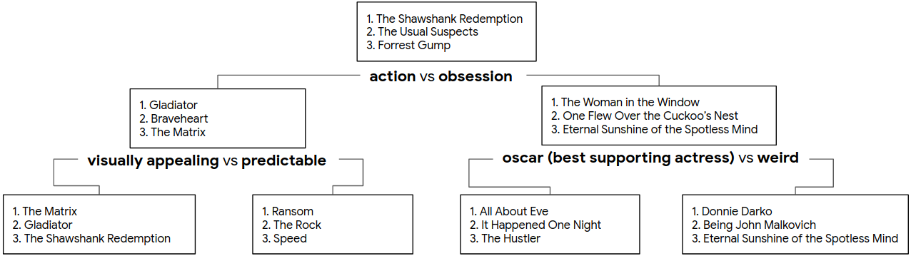
To give an illustration for how elicitation using our method would work in practice, Fig. 7 shows the elicitation queries and recommendations found by , for the single-attribute pairwise comparison case.