Deadlock Analysis and
Resolution for Multi-Robot Systems
(Extended Version)

Abstract

Collision avoidance for multirobot systems is a well studied problem. Recently, control barrier functions (CBFs) have been proposed for synthesizing controllers guarantee collision avoidance and goal stabilization for multiple robots. However, it has been noted reactive control synthesis methods (such as CBFs) are prone to deadlock, an equilibrium of system dynamics causes robots to come to a standstill before reaching their goals. In this paper, we formally derive characteristics of deadlock in a multirobot system uses CBFs. We propose a novel approach to analyze deadlocks resulting from optimization based controllers (CBFs) by borrowing tools from duality theory and graph enumeration. Our key insight is system deadlock is characterized by a force-equilibrium on robots and we show how complexity of deadlock analysis increases approximately exponentially with the number of robots. This analysis allows us to interpret deadlock as a subset of the state space, and we prove this set is non-empty, bounded and located on the boundary of the safety set. Finally, we use these properties to develop a provably correct decentralized algorithm for deadlock resolution which ensures robots converge to their goals while avoiding collisions. We show simulation results of the resolution algorithm for two and three robots and experimentally validate this algorithm on Khepera-IV robots.

1 Introduction

Multirobot systems have been studied thoroughly for solving a variety of complex tasks such as search and rescue [1], sensor coverage [2] and environmental exploration [3]. Global coordinated behaviors result from executing local control laws on individual robots interacting with their neighbors [4], [5]. Typically, the local controllers running on these robots are a combination of a task-based controller responsible for completion of a primary objective and a reactive collision avoidance controller. However, including a hand-engineered safety control no longer guarantees the original task will be satisfied [6]. This problem becomes all the more pronounced when the number of robots increases. Motivated by this bottleneck, our paper focuses on an algorithmic analysis of the performance-safety trade-offs result from augmenting a task-based controller with collision avoidance constraints as done using CBF based quadratic programs (QPs) [7]. Although CBF-QPs mediate between safety and performance in a rigorous way, yet ultimately they are distributed local controllers. Such approaches exhibit a lack of look-ahead, which causes the robots to be trapped in deadlocks as noted in [8, 9, 10]. In deadlock, the robots stop while still being away from their goals and persist in this state unless intervened.

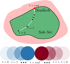
Figure 1: Two robots moving towards each other fall in deadlock. System state converges to the boundary of safe set.

This occurs because robots reach a state where conflict becomes inevitable, i.e. a control favoring goal stabilization will violate safety (see red dot in Fig. 1). Hence, the only feasible strategy is to remain static. Although small perturbations can steer the system away from deadlock, there is no guarantee robots will not fall back in deadlock. To circumvent these issues, this work addresses the following technical questions:

1. What are the characteristics of a system in deadlock ?

2. What all geometric configurations of robots are admissible in deadlock ?

3. How can we leverage this information to provably exit deadlock using decentralized controllers?

To address these questions, we first review technical definitions for CBF based QPs [10] to synthesize controllers for collision avoidance and goal stabilization in section 3. In section 4, we recall the definition of deadlock and use KKT conditions to motivate a novel set theoretic interpretation of deadlock with an eye towards devising controllers evade/exit this set. We use graph enumeration to highlight the combinatorial complexity of geometric configurations of robots admissible in deadlock. Following this development, in section 5 and section 6, we focus on the easier to analyze cases for two and three robots respectively and examine mathematical properties of the deadlock set for these cases. We show this set is on the boundary of the safety set, is non-empty and bounded. In section 7, we show how to design a provably-correct decentralized controller to make the robots exit deadlock. We demonstrate this strategy on two and three robots in simulation, and experimentally on Khepera-IV robots. Finally, we conclude with directions for future work.

2 Prior Work

Several existing methods provide inspiration for the results presented here. Of these, two are especially relevant: in the first category, we describe prior methods for collision avoidance and in the second, we focus on deadlock resolution.

2.1 Prior Work on Avoidance Control

Avoidance control is a well-studied problem with immediate applications for planning collision-free motions for multirobot systems. Classical avoidance control assumes a worst case scenario with no cooperation between robots [11, 12] Cooperative collision avoidance is explored in [13, 14] where avoidance control laws are computed using value functions. Velocity obstacles have been proposed in [15] for motion planning in dynamic environments. They select avoidance maneuvers outside of robot’s velocity obstacles to avoid static and moving obstacles by means of a tree-search. While this method is prone to undesirable oscillations, the authors in [16, 17, 18] propose reciprocal velocity obstacles are immune to such oscillations. More recently, control barrier function based controllers have been used in [6, 10] to mediate between safety and performance using QPs.

2.2 Prior Work on Deadlock Resolution

The importance of coordinating motions of multiple robots while simultaneously ensuring safety, performance and deadlock prevention has been acknowledged in works as early as in [9]. Here, authors proposed scheduling algorithms to asynchronously coordinate motions of two manipulators to ensure their trajectories remain collision and deadlock free. In the context of mobile robots, [19] identified the presence of deadlocks in a cooperative scenario using mobile robot troops. To the best of our knowledge, [20] were the first to propose algorithms for deadlock resolution specifically for multiple mobile robots. Their strategy for collision avoidance modifies planned paths by inserting idle times and resolves deadlocks by asking the trajectory planners of each robot to plan an alternative trajectory until deadlock is resolved. Authors in [21] proposed coordination graphs to resolve deadlocks in robots navigating through narrow corridors. [10, 22] added perturbation terms to their controllers for avoiding deadlock.
         Differently from these, we characterize analytical properties of system states when in deadlock. We explicitly analyze controls from CBF based QPs and demonstrate intuitive explanations for systems in deadlock are indeed recovered using duality. Our analysis can be extended to reveal bottlenecks of any optimization based controller synthesis method. Additionally, we use graph enumeration to highlight the complexity of this analysis. We do not consider additive perturbations for resolving deadlocks, since there are no formal guarantees. Instead, we use feedback linearization and the geometric properties recovered from duality to guide the design of a provably correct controller ensures safety, performance and deadlock resolution.

3 Avoidance Control with CBFs: Review

In this section, we review CBF based QPs used for synthesizing controllers mediate between safety (collision avoidance) and performance (goal-stabilization) for multirobot systems. We refer the reader to [10] for a comprehensive treatment on this subject, since our work builds on top of their approach. Assume we have $N$ mobile robots, each of which follows double-integrator dynamics:

$$\left[\begin{matrix}\dot{\boldsymbol{p}}_{i}\\ \dot{\boldsymbol{v}}_{i}\end{matrix}\right] =\left[\begin{matrix}\dot{\boldsymbol{v}}_{i}\\ \boldsymbol{0}\end{matrix}\right]+\left[\begin{matrix}\boldsymbol{\mbox{O}}\\ \mathbf{I}\end{matrix}\right]\boldsymbol{u}_{i},$$ (1)

where $\boldsymbol{p}_{i}=(x_{i},y_{i})\in\mathbb{R}^{2}$ represents the position of robot $i$, $\boldsymbol{v}_{i}\in\mathbb{R}^{2}$ represents its velocity and $\boldsymbol{u}_{i}\in\mathbb{R}^{2}$ represents the acceleration (i.e. control). The collective state of robot $i$ is denoted by $\boldsymbol{z}_{i}=(\boldsymbol{p}_{i},\boldsymbol{v}_{i})$ and the collective state of the multirobot system is denoted as $\boldsymbol{Z}=(\boldsymbol{z}_{1},\boldsymbol{z}_{2},\dots,\boldsymbol{z}_{N})$. Assume each robot has maximum allowable acceleration limits $|\boldsymbol{u}_{i}|\leq\alpha_{i}$ represent actuator constraints. The problem of goal stabilization with avoidance control requires each robot $i$ must reach a goal $\boldsymbol{p}_{d_{i}}$ while avoiding collisions with every other robot $j\neq i$. For reaching a goal, assume there is a prescribed PD controller $\hat{\boldsymbol{u}}_{i}(\boldsymbol{z}_{i})=-k_{p}(\boldsymbol{p}_{i}-\boldsymbol{p}_{d_{i}})-k_{v}\boldsymbol{v}_{i}$ with $k_{p}$,$k_{v}>0$. This controller is chosen as a nominal reference controller because by itself, it ensures exponential stabilization of each robot to its goal. However, there is no guarantee the resulting trajectories will be collision free.

Based on [10], a safety constraint is formulated for every pair of robots to ensure mutually collision free motions. This constraint is mathematically posed by defining a function maps the joint state space of robots $i\mbox{ and }j$ to a real-valued safety index i.e. $h:\mathbb{R}^{4}\times\mathbb{R}^{4}\longrightarrow\mathbb{R}$. For a desired safety margin distance $D_{s}$, this index is defined as

$$h_{ij}=\sqrt{2(\alpha_{i}+\alpha_{j})(\left\lVert\Delta\boldsymbol{p}_{ij}\right\rVert-D_{s})}+\frac{\Delta\boldsymbol{p}^{T}_{ij}\Delta\boldsymbol{v}_{ij}}{\left\lVert\Delta\boldsymbol{p}_{ij}\right\rVert}.$$ (2)

Robots $i\mbox{ and }j$ are considered to be collision-free if their states $(\boldsymbol{z}_{i},\boldsymbol{z}_{j})$ are such $h_{ij}(\boldsymbol{z}_{i},\boldsymbol{z}_{j})\geq 0$. We define “safe set” as the 0-level superset of $h_{ij}$ i.e. $\mathcal{C}_{ij}\coloneqq\{(\boldsymbol{z}_{i},\boldsymbol{z}_{j})\in\mathbb{R}^{8}\mid h_{ij}(\boldsymbol{z}_{i},\boldsymbol{z}_{j})\geq 0$}. The boundary of the safe set is

$$\partial\mathcal{C}_{ij}=\{(\boldsymbol{z}_{i},\boldsymbol{z}_{j})\in\mathbb{R}^{4}|h(\boldsymbol{z}_{i},\boldsymbol{z}_{j})=0\}$$ (3)

Assuming the initial positions of robots $i\mbox{ and }j$ are in the safe set $\mathcal{C}_{ij}$, we would like to synthesize controls $\boldsymbol{u}_{i}\mbox{ and }\boldsymbol{u}_{j}$ ensure future states of the robots $i\mbox{ and }j$ also stay in $\mathcal{C}_{ij}$. This can be achieved by ensuring

$$\frac{dh_{ij}}{dt}\geq-\kappa(h_{ij}),$$ (4)

where we choose, $\kappa(h)\coloneqq h^{3}$. For the given choice of $h$, 4 can be rewritten as

$$-\Delta\boldsymbol{p}^{T}_{ij}\Delta\boldsymbol{u}_{ij}\leq b_{ij},\mbox{ where}$$ (5)

$$b_{ij}= \left\lVert\Delta\boldsymbol{p}_{ij}\right\rVert h^{3}_{ij}+\frac{(\alpha_{i}+\alpha_{j})\Delta\boldsymbol{p}^{T}_{ij}\Delta\boldsymbol{v}_{ij}}{\sqrt{2(\alpha_{i}+\alpha_{j})(\left\lVert\Delta\boldsymbol{p}_{ij}\right\rVert-D_{s})}}+\left\lVert\Delta\boldsymbol{v}_{ij}\right\rVert^{2}-\frac{(\Delta\boldsymbol{p}^{T}_{ij}\Delta\boldsymbol{v}_{ij})^{2}}{\left\lVert\Delta\boldsymbol{p}_{ij}\right\rVert^{2}}$$ (6)

This constraint is distributed on robots $i\mbox{ and }j$ as:

$$-\Delta\boldsymbol{p}_{ij}^{T}\boldsymbol{u}_{i}\leq\frac{\alpha_{i}}{\alpha_{i}+\alpha_{j}}b_{ij}\mbox{ and }\Delta\boldsymbol{p}_{ij}^{T}\boldsymbol{u}_{j}\leq\frac{\alpha_{j}}{\alpha_{i}+\alpha_{j}}b_{ij}$$ (7)

Therefore, any $\boldsymbol{u}_{i}$ and $\boldsymbol{u}_{j}$ satisfy 7 will ensure collision free trajectories for robots $i\mbox{ and }j$ in the multirobot system. Note these constraints are linear in $\boldsymbol{u}_{i}$ and $\boldsymbol{u}_{j}$ for a given state $(\boldsymbol{z}_{i},\boldsymbol{z}_{j})$. Therefore, the feasible set of controls is convex. Assuming robot $i$ wants to avoid collisions with its $M$ neighbors, there will be $M$ collision avoidance constraints. To mediate between safety and goal stabilization, a QP is posed computes a controller closest to the PD control $\hat{\boldsymbol{u}}_{i}(\boldsymbol{z}_{i})$ (in 2-norm) and satisfies the $M$ collision avoidance constraints:

$$\underset{\boldsymbol{u}_{i}}{\text{minimize}} \left\lVert\boldsymbol{u}_{i}-\hat{\boldsymbol{u}}_{i}(\boldsymbol{z}_{i})\right\rVert^{2}_{2}$$ (8)

subject to $$-\Delta\boldsymbol{p}_{ij}^{T}\boldsymbol{u}_{i}\leq\frac{\alpha_{i}}{\alpha_{i}+\alpha_{j}}b_{ij}\mbox{ }j\in\{1,\dots,M\}$$

$$|\boldsymbol{u}_{i}|\leq\boldsymbol{\alpha}_{i}$$

This QP has $(M+4)$ constraints ($M$ from collision avoidance with $M$ neighbors and four from acceleration limits). Each robot $i$ executes a local version of this QP and computes its optimal $\boldsymbol{u}^{*}_{i}$ at every time step. As long as the QP remains feasible, the generated control $\boldsymbol{u}^{*}_{i}$ ensures collision avoidance of robot $i$ with its neighbors. In the next section, we derive an analytical expression for $\boldsymbol{u}^{*}_{i}$ as a function of $(\boldsymbol{z}_{1},\dots,\boldsymbol{z}_{N})$ to analyze the closed-loop dynamics of the ego robot and use this to investigate the incidence of deadlocks resulting from this technique.

4 Analysis of $N$ Robot Deadlock

We reviewed the formulation of multirobot collision avoidance and goal stablization using the framework of CBF based QPs. In this section, we will show this approach can result in deadlocks (depending on the initial conditions and goals of robots). We want to analyze qualitative properties of a robot in deadlock. Towards end, we will investigate the KKT conditions [23] of the problem in 8. Our goal is to use these conditions to compute properties of geometric configurations of robots in deadlock and then exploit these properties to make the robots exit deadlock. Fig. 2 shows the states of two robots have fallen in deadlock while executing controllers based on 8. Notice from Fig. 2(a) the positions of robots have converged, but not to their respective goals. Therefore, the outputs from the prescribed PD controller will still be non-zero after convergence. However, the control inputs from 8 have already converged to zero Fig. 2(b). From these observations, deadlock is defined as follows [10]

Definition 1.

A robot $i$ is in deadlock if $\boldsymbol{u}^{*}_{i}=0$, $\boldsymbol{v}_{i}=0$, $\hat{\boldsymbol{u}}_{i}\neq 0$ and $\boldsymbol{p}_{i}\neq\boldsymbol{p}_{d_{i}}$

In simpler terms, for a robot to be in deadlock, it should be static i.e. its velocity should be zero, and the output from the QP based controller should also be zero, even though the reference PD controller reports non-zero acceleration since the robot is not at its intended goal. We now look at the KKT conditions for the optimization problem in 8.

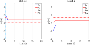
(a) Positions

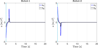
(b) Accelerations (control inputs)

Figure 2: Positions and accelerations of robots falling in deadlock. Note $\lim_{t\rightarrow\infty}p_{x,y}\neq p_{d_{x,y}}$ yet $\lim_{t\rightarrow\infty}a_{x,y}=0$. Video: https://tinyurl.com/y4ylzwh8

4.1 KKT Conditions

Recall each robot $i$ computes a control by solving a local QP as in 8. Define $\boldsymbol{a}_{j}\coloneqq-\Delta\boldsymbol{p}_{ij}$ and $\hat{b}_{j}=\frac{\alpha_{i}}{\alpha_{i}+\alpha_{j}}b_{ij}$.We will drop subscript $i$ and implicitly assume the QP is being solved for the ego robot. Hence, we rewrite 8 as:

$$\underset{\boldsymbol{u}}{\text{minimize}} \left\lVert\boldsymbol{u}-\hat{\boldsymbol{u}}\right\rVert^{2}_{2}$$ (9)

subject to $$\widetilde{A}\boldsymbol{u}\leq\widetilde{\boldsymbol{b}}$$

where $\tilde{A}\coloneqq(\boldsymbol{a}^{T}_{1};\dots;\boldsymbol{a}^{T}_{M};\boldsymbol{e}^{T}_{1};\dots;-\boldsymbol{e}^{T}_{2})$ and $\tilde{\boldsymbol{b}}\coloneqq(\hat{b}_{1};\dots;\hat{b}_{M};\alpha;\dots;\alpha)$. Let $\tilde{\boldsymbol{a}}_{k}$ denote the $k$’th row of $\tilde{A}$ and $\tilde{b}_{k}$ denote the $k$’th element of $\tilde{\boldsymbol{b}}$. The Lagrange dual function for 9 is

$$L(\boldsymbol{u},\boldsymbol{\mu})=\left\lVert\boldsymbol{u}-\hat{\boldsymbol{u}}\right\rVert^{2}_{2}+\sum_{{k=1}}^{M+4}\mu_{k}(\boldsymbol{\tilde{a}}^{T}_{k}\boldsymbol{u}-\tilde{b}_{k})$$ (10)

Let $(\boldsymbol{u}^{*},\boldsymbol{\mu}^{*})$ be the optimal primal-dual solution to 9. The KKT conditions are

1. Stationarity: $\nabla_{\boldsymbol{u}}L(\boldsymbol{u},\boldsymbol{\mu})|_{(\boldsymbol{u}^{*},\boldsymbol{\mu}^{*})}=\boldsymbol{0}$

   $$\implies\boldsymbol{u}^{*}=\hat{\boldsymbol{u}}-\frac{1}{2}\sum_{k=1}^{M+4}\mu^{*}_{k}\boldsymbol{\tilde{a}}^{T}_{k}.$$ (11)

2. Primal Feasibility

   $$\tilde{\boldsymbol{a}}^{T}_{k}\boldsymbol{u}^{*}\leq\tilde{b}_{k}\mbox{ }\forall k\in\{1,2,\dots,M+4\}$$ (12)

3. Dual Feasibility

   $${\mu^{*}_{k}}\geq 0\mbox{ }\forall k\in\{1,2,\dots,M+4\}$$ (13)

4. Complementary Slackness

   $$\mu^{*}_{k}\cdot(\boldsymbol{\tilde{a}}^{T}_{k}\boldsymbol{u}^{*}-\tilde{b}_{k})=0\mbox{ }\forall k\in\{1,2,\dots,M+4\}$$ (14)

Define the set of active and inactive constraints as follows:

$$\mathcal{A}(\boldsymbol{u}^{*})=\{k\in\{1,2,\dots,M+4\}\mid\boldsymbol{\tilde{a}}^{T}_{k}\boldsymbol{u}^{*}=\tilde{b}_{k}\}$$ (15)

$$\mathcal{IA}(\boldsymbol{u}^{*})=\{k\in\{1,2,\dots,M+4\}\mid\boldsymbol{\tilde{a}}^{T}_{k}\boldsymbol{u}^{*}<\tilde{b}_{k}\}$$ (16)

Using complementary slackness from 14, we deduce

$$\mu^{*}_{k}=0\mbox{ $\forall k$}\in\mathcal{IA}(\boldsymbol{u}^{*})$$ (17)

Therefore, we can restrict the sum in 11 to only the set of active constraints

$$\boldsymbol{u}^{*}=\hat{\boldsymbol{u}}-\frac{1}{2}\sum_{k\in\mathcal{A}(\boldsymbol{u}^{*})}\mu^{*}_{k}\boldsymbol{\tilde{a}}^{T}_{k}$$ (18)

4.2 KKT Conditions for the deadlock case

From Def. 1, we know in deadlock, $\boldsymbol{u}^{*}=\boldsymbol{0}$, $\hat{\boldsymbol{u}}\neq 0$ and $\boldsymbol{v}=\boldsymbol{0}$. We conclude:

1. In deadlock, $\boldsymbol{u}^{*}\neq\hat{\boldsymbol{u}}$ i.e. the solution to the QP is not equal to the prescribed PD controller (which means $\hat{\boldsymbol{u}}$ is infeasible in deadlock i.e. $\boldsymbol{a}^{T}\hat{\boldsymbol{u}}\nleq\hat{b}$).

2. $\boldsymbol{u}^{*}=\boldsymbol{0}\implies\boldsymbol{u}^{*}\neq\pm\boldsymbol{\alpha}$. This implies at least the last four constraints in $\tilde{A}\boldsymbol{u}\leq\tilde{b}$ are inactive i.e. $\{M+1,M+2,M+3,M+4\}\in\mathcal{IA}(\boldsymbol{u}^{*})$ in deadlock.

Using these observations, we rewrite the KKT conditions for the deadlock case:

1. Stationarity: $\nabla_{\boldsymbol{u}}L(\boldsymbol{u},\boldsymbol{\mu})|_{(\boldsymbol{0},\boldsymbol{\mu}^{*})}=\boldsymbol{0}$

   $$\implies\hat{\boldsymbol{u}}=\frac{1}{2}\sum_{k\in\mathcal{A}(\boldsymbol{u}^{*})}\mu^{*}_{k}\boldsymbol{\tilde{a}}^{T}_{k}$$ (19)

2. Primal Feasibility

   $$\tilde{b}_{k}\geq 0\mbox{ }\forall k\in\{1,2,\dots,M+4\}$$ (20)

3. Dual Feasibility

   $${\mu^{*}_{k}}\geq 0\mbox{ }\forall k\in\{1,2,\dots,M+4\}$$ (21)

4. Complementary Slackness

   $$\mu^{*}_{k}\cdot(\tilde{\boldsymbol{a}}^{T}_{k}\boldsymbol{u}^{*}-\tilde{b}_{k})=0$$

   $$\implies\mu^{*}_{k}\cdot\tilde{b}_{k}=0\mbox{ $\forall$}j\in\{1,2,\dots,M+4\}$$ (22)

Based on these conditions, we will now motivate a set-theoretic interpretation of deadlock. Assume the state of the ego robot is $\boldsymbol{z}=(\boldsymbol{p},\boldsymbol{v})$ and it has $M$ neighbors denoted as $\boldsymbol{Z}_{nb.}$. Define $P\in\mathbb{R}^{2\times 4}$ and $V\in\mathbb{R}^{2\times 4}$ appropriately to extract the position and velocity components from $\boldsymbol{z}$ i.e. $\boldsymbol{p}=P\boldsymbol{z}$ and $\boldsymbol{v}=V\boldsymbol{z}$. Finally, define $\mathcal{D}$ as:

$$\mathcal{D}(\boldsymbol{z}\mid\boldsymbol{Z}_{nb.})=\{\boldsymbol{z}\in\mathbb{R}^{4}\mid{\boldsymbol{u}^{*}}(\boldsymbol{z})=0,\hat{\boldsymbol{u}}(\boldsymbol{z})\neq 0,V\boldsymbol{z}=0,\mu_{k}^{*}(\boldsymbol{Z})>0\mbox{ $\forall$ }k\in\mathcal{A}(\boldsymbol{u^{*}})\}$$ (23)

The set $\mathcal{D}$ is defined as the set of all states of the ego robot which satisfy the criteria of being in deadlock. We have combined the conditions of deadlock into a set theoretic definition. Note for each robot, its set of deadlock states depends on the states of its neighboring robots. This is because the Lagrange multipliers depend on the states of all robots. The motivation behind stating this definition is to interpret deadlock as a bonafide set in the state space of the ego robot and derive a control strategy makes the robot evade/exit this set. We now rewrite this definition in more easily interpretable conditions. From 18 and 19, note

$${\boldsymbol{u}}^{*}(\boldsymbol{z})=0\iff\hat{\boldsymbol{u}}(\boldsymbol{z})=\frac{1}{2}\sum_{k\in\mathcal{A}({\boldsymbol{u}^{*}}(\boldsymbol{z}))}\mu^{*}_{k}\boldsymbol{\tilde{a}}_{k}$$ (24)

Since $\boldsymbol{\tilde{a}}_{k}=-\Delta\boldsymbol{p}_{ik}=-P(\boldsymbol{z}-\boldsymbol{z}_{k})$, we rewrite 24 as:

$${\boldsymbol{u}}^{*}(\boldsymbol{z})=0\iff\hat{\boldsymbol{u}}(\boldsymbol{z})=-\frac{1}{2}\sum_{k\in\mathcal{A}({\boldsymbol{u}^{*}}(\boldsymbol{z}))}\mu^{*}_{k}P(\boldsymbol{z}-\boldsymbol{z}_{k})$$ (25)

We will use this condition to replace the ${\boldsymbol{u}}^{*}(\boldsymbol{z})=0$ criterion in the def. of $\mathcal{D}$ in (23). Secondly, we know prescribed controller $\hat{\boldsymbol{u}}(\boldsymbol{z})$ is a PD controller. Define the goal state as $\boldsymbol{z}_{d}=(\boldsymbol{p}_{d},\boldsymbol{0})$. Noting $\hat{\boldsymbol{u}}(\boldsymbol{z})\neq 0$ and $\boldsymbol{v}=\mathbf{0}$,

$$\hat{\boldsymbol{u}}(\boldsymbol{z})=-k_{p}(\boldsymbol{p}-\boldsymbol{p}_{d})-k_{v}\boldsymbol{v}\neq\mathbf{0}\iff P(\boldsymbol{z}-\boldsymbol{z}_{d})\neq\mathbf{0}$$ (26)

This criterion is restating in deadlock the ego robot is not at its goal. The final condition is the velocity of the ego robot is zero i.e. $\boldsymbol{v}=\boldsymbol{0}\iff V\boldsymbol{z}=\boldsymbol{0}$. Combining these conditions, we rewrite the definition of the deadlock from 23 as follows:

$$\mathcal{D}(\boldsymbol{z}\mid\boldsymbol{Z}_{nb.})=\{\boldsymbol{z}\in\mathbb{R}^{4}| \hat{\boldsymbol{u}}(\boldsymbol{z})=-\frac{1}{2}\sum_{k\in\mathcal{A}({\boldsymbol{u}^{*}}(\boldsymbol{z}))}\mu^{*}_{k}P(\boldsymbol{z}-\boldsymbol{z}_{k}),P(\boldsymbol{z}-\boldsymbol{z}_{d})\neq 0,V\boldsymbol{z}=0,$$

$$\mu_{k}^{*}>0\mbox{ $\forall$ }k\in\mathcal{A}(\boldsymbol{u^{*}}(\boldsymbol{z}))\}$$ (27)

Building on the definition of one robot deadlock, we motivate system deadlock to be the set of states where all robots are in deadlock and is defined as

$$\mathcal{D}_{system}= \{(\boldsymbol{z}_{1},\boldsymbol{z}_{2},\cdots,\boldsymbol{z}_{N})\in\mathbb{R}^{4N}\mid\boldsymbol{z}_{i}\in\mathcal{D}(\boldsymbol{z}_{i}\mid\boldsymbol{Z}^{i}_{nb.})\mbox{ }\forall i\in\{1,2,\cdots,N\})$$ (28)

For the rest of the paper, we will focus our analysis on system deadlock. This is because the case where only a subset of robots are in deadlock can be decomposed into subproblems where a subset is in system deadlock and the remaining robots free to move. The next section focuses on the geometric complexity analysis of system deadlock.

4.3 Graph Enumeration based Complexity Analysis of Deadlock

The Lagrange multipliers $\mu^{*}_{k}$ are in general, a nonlinear function of the state of robots $\boldsymbol{z}$. Their values depend on which constraints are active/inactive (an example calculation is shown in section 5). An active constraint will in-turn determine the set of possible geometric configurations the robots can take when they are in deadlock (sections 5 and 6) and this in turn will guide the design of our deadlock resolution algorithm (section 7). Therefore, we are interested in deriving all possible combinations of active/inactive constraints the robots can assume once in deadlock. But first we derive upper and lower bounds for the number of valid configurations in system deadlock.

We can interpret an active collision avoidance constraint between robots $i$ and $j$ as an undirected edge between vertices $i$ and $j$ in a graph formed by $N$ labeled vertices, where each vertex represents a robot. The following property (which follows from symmetry) allows the edges to be undirected.

Lemma 4.1.

If robot $i$ and $j$ are both in deadlock and $i^{\prime}s$ constraint with $j$ is active (inactive), then $j^{\prime}s$ constraint with $i$ is also active (inactive).

4.3.1 Upper Bound

Given $N$ vertices, there are ${}^{N}C_{2}$ distinct pairs of edges possible. The overall system can have any subset of those edges. Since a set with ${}^{N}C_{2}$ members has $2^{{}^{N}C_{2}}$ subsets, we conclude there are $2^{{}^{N}C_{2}}$ possible graphs. In other words, given $N$ robots, the number of configurations are admissible in deadlock is $2^{{}^{N}C_{2}}$. However, this number is an upper bound because it includes cases where a given vertex can be disconnected from all other vertices, which is not valid in system deadlock as shown next.

4.3.2 Lower Bound

We further impose the restriction each vertex in the graph have at-least one edge i.e. each robot have at-least one constraint active with some other robot. This is because if a robot has no active constraints i.e. $\mu^{*}_{k}=0$ $\forall k$ then from 24, we will get $\boldsymbol{u}^{*}(\boldsymbol{z})=\hat{\boldsymbol{u}}(\boldsymbol{z})=\boldsymbol{0}$ which would contradict the definition of deadlock for robot and hence contradict system deadlock. blackFrom this observation, it follows the set of graphs are valid in system deadlock is a superset of connected simple graphs can be formed by $N$ labeled vertices. This is because there could be graphs are not simply connected yet admissible in deadlock. While this argument is based on algebraic qualifiers resulting from the ‘edge’ interpretation of collision avoidance constraints, it is possible some simply connected graphs may not be geometrically feasible due to restrictions imposed by Euclidean geometry. Graphs are (a) simply-connected (to enforce deadlock for each robot), (b) have $N$ labelled vertices (since each robot has an ID), (c) are embedded in $\mathbb{R}^{2}$ (since the robots/environment are planar), (d) have Euclidean distance between connected vertices equal to $D_{s}$, (e) between unconnected vertices greater than $D_{s}$, and (f) have at-least one or two edges per vertex, necessarily represent admissible geometric configurations of robots in system deadlock. The reason for qualifiers (d) and (e) is explained in the proof of theorem 5.1. (f) is needed because the decision variables in 9 are in $\mathbb{R}^{2}$, so there can be one or two active constraints (possibly more) per ego robot. The number of graphs meeting qualifiers (a) and (b) can be obtained using the following recurrence relation [24]

$$d_{N}=2^{{}^{N}C_{2}}-\frac{1}{N}\sum_{k=1}^{N-1}k\mbox{ }{{}^{N}C_{k}}2^{{}^{N-k}C_{2}}d_{k}$$ (29)

For $N=\{1,\mbox{ }2,\mbox{ }3,\mbox{ }4\}$, this number is $\{1,\mbox{ }1,\mbox{ }4,\mbox{ }38\}$. The number of graphs meeting qualifiers (a), (c) and (d) can be obtained by calculating the number of connected matchstick graphs on $N$ nodes [25]. The number of graphs meeting (b) and (d) was obtained in [26] and is exponential in $N^{2}$ (for unit distance graphs). A lower bound for graphs satisfying all qualifiers (a)-(f) can be shown to be $0.5(N+1)(N-1)!$ as follows ($N\geq 3$). Consider a cyclic graph whose each node is the vertex of an $N$ regular polygon with side $D_{s}$. Such a graph necessarily satisfies (a)-(f). Re-arrangements of its vertices gives rise to $0.5(N-1)!$ graphs. Likewise, a graph with nodes along an open chain also satisfies (a)-(f), and gives $0.5N!$ rearrangements. Thus, the total is $0.5(N-1)!+0.5N!=0.5(N+1)(N-1)!$ It is well known factorial overtakes exponential, thus highlighting the increase in the number of geometric configurations. Our MATLAB simulations show the exact number of configurations for $N=\{1,\mbox{ }2,\mbox{ }3,\mbox{ }4\}$ are $\{1,\mbox{ }1,\mbox{ }4,\mbox{ }18\}$ whereas our bound gives $\{1,\mbox{ }1,\mbox{ }4,\mbox{ }15\}$. This simulation demonstrates the explosion in the number of possible geometric configurations are admissible in system deadlock with increasing number of robots. Therefore for further analysis, we will restrict to the case of two and three robots.

5 Two-Robot Deadlock

In section 4, we proposed a set-theoretic definition of deadlock for a specific robot in an $N$ robot system. In this section, we will refine the KKT conditions derived in section 4.2 for the case of two robots in the system. This setting reveals several important underlying characteristics of the system are extendable to the $N$ robot case, as will be shown for $N=3$. One key feature of a two-robot system is a single robot by itself cannot be in deadlock i.e. either both robots are in deadlock or neither. This is because the sole collision avoidance constraint is symmetric due to Lemma 1. Hence, a two-robot system can only exhibit system deadlock. Additionally since the ego robot avoids collision only with the one other robot, there is no sum in 24 i.e.

$${\boldsymbol{u}}^{*}(\boldsymbol{z})=0\iff\hat{\boldsymbol{u}}(\boldsymbol{z})=\frac{1}{2}\mu^{*}\boldsymbol{a}$$ (30)

The left hand side of this equation is $\hat{\boldsymbol{u}}(\boldsymbol{z})=-k_{p}(\boldsymbol{p}_{ego}-\boldsymbol{p}_{d})$. The right hand side is $\frac{1}{2}\mu^{*}\boldsymbol{a}=-\frac{1}{2}\mu^{*}(\boldsymbol{p}_{ego}-\boldsymbol{p}_{neighbor})$. Writing this another way, we have $-k_{p}(\boldsymbol{p}_{ego}-\boldsymbol{p}_{d})+\frac{1}{2}\mu^{*}(\boldsymbol{p}_{ego}-\boldsymbol{p}_{neighbor})=\boldsymbol{0}$. The first term as represents an attractive force pulls the ego robot towards goal $\boldsymbol{p}_{d}$. Since $\mu^{*}>0$, the second term represents a repulsive force pushing the ego robot away from its neighbor. Thus, system deadlock occurs when the net force due to attraction and repulsion on each robot vanishes (see Fig. 3(a)). We now define the system deadlock set $\mathcal{D}_{system}$ using sections 4.2 and 28:

$$\mathcal{D}_{system}= \{(\boldsymbol{z}_{1},\boldsymbol{z}_{2})\in\mathbb{R}^{8}\mid\boldsymbol{\hat{u}}_{1}=\frac{1}{2}\mu^{*}_{1}\boldsymbol{a}_{1},\mbox{ }\boldsymbol{\hat{u}}_{2}=\frac{1}{2}\mu^{*}_{2}\boldsymbol{a}_{2},\mbox{ }\mu^{*}_{1}>0,\mbox{ }\mu^{*}_{2}>0,\mbox{ }$$

$$(P(\boldsymbol{z}_{1}-\boldsymbol{z}_{d_{1}}),P(\boldsymbol{z}_{2}-\boldsymbol{z}_{d_{2}}))\neq(\boldsymbol{0},\boldsymbol{0}),\mbox{ }(V\boldsymbol{z}_{1},V\boldsymbol{z}_{2})=(\boldsymbol{0},\boldsymbol{0})\}.$$ (31)

where $\boldsymbol{a}_{1}=-\boldsymbol{a}_{2}=-(\boldsymbol{p}_{1}-\boldsymbol{p}_{2})$. Next, we derive analytical expressions for the Lagrange multipliers $\mu^{*}_{1},\mu^{*}_{2}$. Depending on whether the collision avoidance constraint is active/inactive at the optimum, there are two cases:
Case 1: The constraint $\boldsymbol{a}^{T}\boldsymbol{u}\leq\hat{b}$ is active at $\boldsymbol{u}=\boldsymbol{u}^{*}$ i.e. $\boldsymbol{a}^{T}\boldsymbol{u}^{*}=\hat{b}$

$$\implies\boldsymbol{a}^{T}\bigg{(}\hat{\boldsymbol{u}}-\frac{1}{2}\mu^{*}\boldsymbol{a}\bigg{)}=\hat{b}$$

$$\implies\mu^{*}=2\frac{\boldsymbol{a}^{T}\hat{\boldsymbol{u}}-\hat{b}}{\left\lVert\boldsymbol{a}\right\rVert^{2}_{2}}$$ (32)

Case 2: The constraint $\boldsymbol{a}^{T}\boldsymbol{u}\leq\hat{b}$ is inactive at $\boldsymbol{u}=\boldsymbol{u}^{*}$ i.e. $\boldsymbol{a}^{T}\boldsymbol{u}^{*}<\hat{b}$. From complementary slackness, it follows $\mu^{*}=0$ and hence $\boldsymbol{u}^{*}=\hat{\boldsymbol{u}}$. However, this contradicts the definition of deadlock. Hence, case 2 can never arise in deadlock.

5.1 Characteristics of two-robot deadlock

We now analyze qualitative properties of the system deadlock set towards synthesizing a controller will enable the robots to exit this set. We will show when deadlock occurs, (1) the two robots are separated by the safety distance, (2) deadlock set is non-empty and (3) bounded and of measure zero.

Theorem 5.1 (Safety Margin Apart).

In deadlock, the two robots are separated by the safety distance and the robots are on the verge of violating safety (see Fig. 1, 3(a))

Proof 5.2.

In section 5, we proved the collision avoidance constraint is active in deadlock. Since both robots are in deadlock, we know both of their collision avoidance constraints are active i.e. $\boldsymbol{a}^{T}_{1}\boldsymbol{u}_{1}^{*}=\hat{b}_{12}\mbox{ , }\boldsymbol{a}^{T}_{2}\boldsymbol{u}_{2}^{*}=\hat{b}_{21}$ and $\boldsymbol{u}_{1}^{*}=\boldsymbol{0}$ and $\boldsymbol{u}_{2}^{*}=\boldsymbol{0}$. This implies $\hat{b}_{12}=\hat{b}_{21}=0$. Using 6 and 7 and in deadlock, $(\boldsymbol{v}_{1},\boldsymbol{v}_{2})=(\boldsymbol{0},\boldsymbol{0})$ we get

$$\hat{b}_{12}=\frac{\alpha_{1}}{\alpha_{1}+\alpha_{2}}\left\lVert\Delta\boldsymbol{p}_{12}\right\rVert h^{3}_{12}=0\implies h_{12}=0$$ (33)

Recall $h_{12}$ from 2 and using $(\boldsymbol{v}_{1},\boldsymbol{v}_{2})=(\boldsymbol{0},\boldsymbol{0})$, we get

$$h_{12}(\boldsymbol{z}_{1},\boldsymbol{z}_{2})=\sqrt{2(\alpha_{1}+\alpha_{2})(\left\lVert\Delta\boldsymbol{p}_{12}\right\rVert-D_{s})}$$ (34)

Therefore, $h_{12}=0\iff\left\lVert\Delta\boldsymbol{p}_{12}\right\rVert=D_{s}$. Assuming QP is feasible, we disregard $\left\lVert\Delta\boldsymbol{p}_{12}\right\rVert=0$. Therefore, $\left\lVert\Delta\boldsymbol{p}_{12}\right\rVert=D_{s}$. Additionally, recalling the definition from $\partial\mathcal{C}$ from 3 we deduce , in deadlock, $(\boldsymbol{z}_{1},\boldsymbol{z}_{2})\in\partial\mathcal{C}$ i.e. $\mathcal{D}_{system}\subset\partial\mathcal{C}$.

This result confirms our intuition, because if the robots are separated by more than the safety distance, then they will have wiggle room to move because they are not at their goals and $\hat{\boldsymbol{u}}\neq\boldsymbol{0}$. However, the ability to move, albeit with small velocity would contradict the definition of deadlock. We now propose a family of states are always in the system deadlock set $\mathcal{D}_{system}$.

Theorem 5.3 ($\mathcal{D}_{system}$ is Non-Empty).

$\forall\mbox{ }k_{p},k_{v},D_{s}>0,\exists$ a family of states $(\boldsymbol{z}^{*}_{1},\boldsymbol{z}^{*}_{2})\in\mathcal{D}_{system}$. These states are such the robots and their goals are all collinear.

Proof 5.4.

To prove this theorem, we propose a set of candidate states $(\boldsymbol{z}^{*}_{1},\boldsymbol{z}^{*}_{2})$ and show they satisfy the definition of deadlock section 5. See Fig. 3(a) for an illustration of geometric quantities referred to in this proof.

Let $\boldsymbol{p}^{*}_{1}=\alpha\boldsymbol{p}_{d_{1}}+(1-\alpha)\boldsymbol{p}_{d_{2}}$ and $\boldsymbol{p}^{*}_{2}=\boldsymbol{p}^{*}_{1}-D_{s}\hat{e}_{\beta}$ where $\beta=\mbox{tan}^{-1}(\frac{y_{d_{2}}-y_{d_{1}}}{x_{d_{2}}-x_{d_{1}}})$ and $\alpha\in(0,1)$. Note $\boldsymbol{p}^{*}_{1},\boldsymbol{p}^{*}_{2},\boldsymbol{p}_{d_{1}},\boldsymbol{p}_{d_{2}}$ are collinear by construction. Let $\boldsymbol{z}^{*}_{1}=(\boldsymbol{p}^{*}_{1},\boldsymbol{0})$ and $\boldsymbol{z}^{*}_{2}=(\boldsymbol{p}^{*}_{2},\boldsymbol{0})$. Then we will show $\boldsymbol{Z^{*}}=(\boldsymbol{z}^{*}_{1},\boldsymbol{z}^{*}_{2})\in\mathcal{D}_{system}$. Note

$$\centering\boldsymbol{a}_{1}\@add@centering =-(\boldsymbol{p}^{*}_{1}-\boldsymbol{p}^{*}_{2})=-D_{s}\hat{e}_{\beta}$$

$$\hat{\boldsymbol{u}}_{1} =-k_{p}(\boldsymbol{p}^{*}_{1}-\boldsymbol{p}_{d_{1}})$$ (35)

From definition, $\hat{e}_{\beta}=\frac{1}{D_{G}}(x_{d_{2}}-x_{d_{1}},y_{d_{2}}-y_{d_{1}})$ where $D_{G}=\left\lVert\boldsymbol{p}_{d_{2}}-\boldsymbol{p}_{d_{1}}\right\rVert$ is the distance between the goals. Therefore, we have

$$\boldsymbol{p}^{*}_{1}-\boldsymbol{p}_{d_{1}} =-(1-\alpha)\boldsymbol{p}_{d_{1}}+(1-\alpha)\boldsymbol{p}_{d_{2}}$$

$$=(1-\alpha)D_{G}\hat{e}_{\beta}$$ (36)

Substituting 5.4 in 5.4 gives

$$\hat{\boldsymbol{u}}_{1}=-k_{p}(1-\alpha)D_{G}\hat{e}_{\beta}$$ (37)

From 5.4 and 37, we deduce Lagrange multiplier $\mu_{1}$

$$\mu_{1} =2\frac{\boldsymbol{a}^{T}_{1}\hat{\boldsymbol{u}}_{1}}{\left\lVert\boldsymbol{a}_{1}\right\rVert^{2}_{2}}=2k_{p}(1-\alpha)\frac{D_{G}}{D_{s}}>0\mbox{ }\forall\alpha\in(0,1)$$

$$\implies\frac{1}{2}\mu_{1}\boldsymbol{a}_{1} =-\frac{1}{2}2k_{p}(1-\alpha)\frac{D_{G}}{D_{s}}D_{s}\hat{e}_{\beta}=\hat{\boldsymbol{u}}_{1}$$ (38)

Hence, in 5.4, we have shown $\hat{\boldsymbol{u}}_{1}=\frac{1}{2}\mu_{1}\boldsymbol{a}_{1}$ which is one condition in the definition of the deadlock set. Similarly, we can show $\hat{\boldsymbol{u}}_{2}=\frac{1}{2}\mu_{2}\boldsymbol{a}_{2}$. Also note in 5.4 we have shown the Lagrange multiplier $\mu_{1}$ is positive, which is another condition in section 5. We can similarly show $\mu_{2}>0$. Finally, note for our choice of states, $\boldsymbol{v}^{*}_{1}=\boldsymbol{v}^{*}_{2}=\boldsymbol{0}$ and we have restricted $\alpha\in(0,1)$ so we can ensure $\boldsymbol{p}^{*}_{i}\neq\boldsymbol{p}_{d_{i}}$ Hence, the proposed states are always in deadlock.

Theorem 5.5 ($\mathcal{D}_{system}$ is bounded).

The system deadlock set is bounded and measure zero.

Proof 5.6.

Following the definition of $\boldsymbol{p}^{*}_{1}$ and $\boldsymbol{p}^{*}_{2}$ from theorem 5.1 and theorem 5.3, we can show when two robots are in deadlock, their positions satisfy

$$\left\lVert\big{(}\boldsymbol{p}_{1}-\boldsymbol{p}_{d_{1}}\big{)}\right\rVert+\left\lVert\big{(}\boldsymbol{p}_{2}-\boldsymbol{p}_{d_{2}}\big{)}\right\rVert=D_{s}+D_{G}$$

This can be verified by straightforward substitution. From this constraint it is evident, the deadlock set is not “large”, bounded and of measure zero. is why, random perturbations are one feasible way to resolve deadlock.

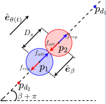
(a) Two Robot Equilibrium

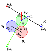
(b) Three Robot Equilibrium

Figure 3: Force Equilibrium in Deadlock

6 Three Robot Deadlock

Following the ideas developed for two robot deadlock, we now describe the three robot case. We will demonstrate properties such as robots being on the verge of safety violation (theorem 6.1) and non-emptiness (theorem 6.3) are retained in this case as well. We are interested in analyzing system deadlock, which occurs when $\boldsymbol{u}^{*}_{i}=\boldsymbol{0}$, $\boldsymbol{v}_{i}=\boldsymbol{0}$ and $\hat{\boldsymbol{u}}_{i}\neq\boldsymbol{0}$ $\forall i\in\{1,2,3\}$. Since we are studying system deadlock, each robot will have at-least one active collision avoidance constraint (each robot has two constraints in total). Note the system deadlock set $\mathcal{D}_{system}$ for three robots is defined analogously to section 5.

Theorem 6.1 (Safety Margin Apart).

In system deadlock, either all three robots are separated by the safety margin or exactly two pairs of robots are separated by the safety margin.

Proof 6.2.

The proof is kept brief because it is similar to the proof of theorem 5.1. Based on the number of constraints are allowed to be active per robot, all geometric configurations can be clubbed in two categories :
Category A - This arises when all collision avoidance constraints of each robot are active i.e. $\boldsymbol{a}^{T}_{ij}\boldsymbol{u}^{*}_{i}=\hat{b}_{ij}=0\iff\left\lVert\Delta\boldsymbol{p}_{ij}\right\rVert=D_{s}\mbox{ }\forall j\in\{1,2,3\}\backslash i$ $\forall i\in\{1,2,3\}$. As a result, each robot is separated by $D_{s}$ from every other robot (Fig. 4(a)).
Category B - This arises when there is exactly one robot with both its constraints active (robot $i$ in Fig. 4(b)), and the remaining two robots ($j$ and $k$) have exactly one constraint active each. Hence, robot $i$ is separated by $D_{s}$ from the other two. After relabeling of indices, category B results in three rearrangements.

Theorem 6.3 (Non-emptiness).

$\forall\mbox{ }k_{p},k_{v},D_{s},R$ $>0$ and $\boldsymbol{p}_{d_{i}}=R\hat{\boldsymbol{e}}_{2\pi(i-1)/3}$ where $i=\{1,2,3\}$, $\exists$ $(\boldsymbol{z}^{*}_{1},\boldsymbol{z}^{*}_{2},\boldsymbol{z}^{*}_{3})\in\mathcal{D}_{system}$ where $\boldsymbol{z}^{*}_{i}=(\boldsymbol{p}^{*}_{i},\boldsymbol{0})$ and $\boldsymbol{p}^{*}_{i}$ is proposed as follows:
Category A: $\boldsymbol{p}^{*}_{i}=\frac{D_{s}}{\sqrt{3}}\hat{\boldsymbol{e}}_{\frac{2\pi(i-1)}{3}+\pi}$ where $i=\{1,2,3\}$
Category B: $\boldsymbol{p}^{*}_{1}=D_{s}\hat{\boldsymbol{e}}_{\pi}$, $\boldsymbol{p}^{*}_{2}=\boldsymbol{0}$, $\boldsymbol{p}^{*}_{3}=D_{s}\hat{\boldsymbol{e}}_{\frac{\pi}{3}}$ if robot $2$ has both constraints active.

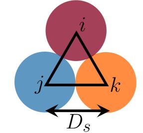
(a) Category A

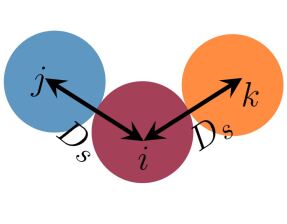
(b) Category B

Figure 4: Geometric configurations in system deadlock of three robots

Proof 6.4.

This proof is similar to the proof of theorem 5.3 so it is skipped. Some remarks:

1. In the statement of this theorem, we have predefined the desired goal positions unlike the statement of theorem 5.3. The candidate positions of the robots we propose are in $\mathcal{D}_{system}$ are valid with respect to these given goals. We have derived a similar non-emptiness result for arbitrary goals but are not including it here for the sake of brevity.

2. For category B, we proposed one set of positions is valid in deadlock, however there is continuous family of positions can be valid in category B. The representation of this family can be found in the appendix in theorem A.1.

7 Deadlock Resolution

We now use the properties of geometric configurations derived in section 5 and section 6 to synthesize a strategy (1) gets the robots out of deadlock, (2) ensures their safety and (3) makes them converge to their goals. One approach to achieve these objectives is to detect the incidence of deadlock while the CBF-QP controller is running on the robots and once detected, any small non-zero perturbation to the control will instantaneously give a non-zero velocity to the robots. Thereafter, CBF-QPs can take charge again and we can hope using this controller the system state will come out of deadlock at-least for a short time. This has two limitations however; firstly, since it was the CBF-QP controller led to deadlock, there is no guarantee the system will not fall back in deadlock again. Secondly, perturbations can violate safety and even lead to degraded performance. Therefore, we propose a controller which ensures goal stabilization, safety and deadlock resolution are met with guarantees. We demonstrate this algorithm for the two and three robot cases. Extension to $N\geq 4$ is left for future work since $N\geq 4$ admits a large number of geometric configurations are valid in deadlock. Refer to Fig. 5 for a schematic of our approach. This algorithm is described here:

(a) Deadlock resolution for two robots

(b) Deadlock resolution for three robots

Figure 5: Deadlock Resolution Algorithm Schematic

1. The algorithm starts by executing controls derived from CBF-QP in Phase 1. This ensures movement of robots to the goals and safety by construction. To detect the incidence of deadlock, we continuously compare $\left\lVert\boldsymbol{u}^{*}\right\rVert,\left\lVert\boldsymbol{v}\right\rVert,\left\lVert\boldsymbol{p}-\boldsymbol{p}_{d}\right\rVert$ against small thresholds. If satisfied, we switch control to phase 2, otherwise, phase 1 continues to operate.

2. In this phase, we rotate the robots around each other to swap positions while maintaining the safe distance.

   1. For the two-robot case, we calculate $\boldsymbol{u}^{1}_{fl}(t)$ and $\boldsymbol{u}^{2}_{fl}(t)$ using feedback linearization (see appendix material) to ensure $\left\lVert\Delta\boldsymbol{p}_{12}\right\rVert=D_{s}$ and rotation ($\ddot{\theta}=-k_{p}(\theta-\beta)-k_{v}\dot{\theta}\implies\Delta\boldsymbol{p}^{T}_{12}\Delta\boldsymbol{v}_{12}=0$) (See Fig. 3(b) for $\theta,\beta$). This rotation and distance invariance guarantees safety i.e. $\ h_{12}=0$. Adding an extra constraint $\boldsymbol{u}^{1}_{fl}+\boldsymbol{u}^{2}_{fl}=\boldsymbol{0}$ still ensures the problem is well posed and additionally makes the centroid static.

   2. For the three-robot case, we calculate $\boldsymbol{u}^{1}_{fl}(t),\boldsymbol{u}^{3}_{fl}(t),\boldsymbol{u}^{3}_{fl}(t)$ to ensure $\left\lVert\Delta\boldsymbol{p}_{12}\right\rVert=\left\lVert\Delta\boldsymbol{p}_{23}\right\rVert=\left\lVert\Delta\boldsymbol{p}_{31}\right\rVert=D_{s}$ and rotation ($\ddot{\theta}=-k_{p}(\theta-\beta)-k_{v}\dot{\theta}\implies\Delta\boldsymbol{p}^{T}_{12}\Delta\boldsymbol{v}_{12}=0$) (See Fig. 3(b) for $\theta,\beta$). This guarantees safety i.e. $h_{12}=h_{23}=h_{31}=0$. Similarly, we impose $\boldsymbol{u}^{1}_{fl}+\boldsymbol{u}^{2}_{fl}+\boldsymbol{u}^{3}_{fl}=\boldsymbol{0}$ to make the centroid static.

3. Once the robots swap their positions, their new positions will ensure prescribed PD controllers will be feasible in the future. Thus, after convergence of Phase 2 (which happens in finite time), control switches to Phase 3, which simply uses the prescribed PD controllers. This phase guarantees the distance between robots is non-decreasing and safety is maintained as we prove in theorem 7.1.

Fig. 6 shows simulation and experimental results from running this strategy on two (6(a)) and three (Fig. 6(c)) robots. Experiments were conducted using Khepera 4 nonholonomic robots (6(b)). Note for nonholnomic robots, we noticed from experiments and simulations deadlock only occurs if the body frames of both robots are perfectly aligned with one another at $t=0$. Since this alignment is difficult to establish in experiments, we simulated a virtual deadlock at $t=0$ i.e. assumed the initial position of robots are ones are in deadlock.

We next prove this strategy ensures resolution of deadlock and convergence of robots to their goals. The proof of this theorem will exploit the geometric properties of deadlock we derived in theorem 5.1 and theorem 5.3. We prove this theorem for $N=2$ since the proof for $N=3$ is a trivial extension of $N=2$.

Theorem 7.1.

Assuming PD controllers are overdamped and $D_{G}>D_{s}$, this strategy ensures (1) the robots will never fall in deadlock and (2) converge to their goals.

Proof 7.2.

We would like to show once phase three control begins, the robots will never fall back in deadlock. We will do this by showing the distance between the robots is non-decreasing, once phase three control starts.

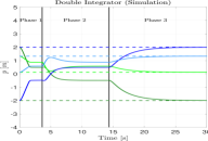
(a) Two Robots Sims.

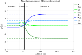
(b) Expmts. with Kheperas.

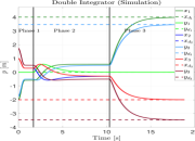
(c) Three Robots Sims.

Figure 6: Positions of robots from deadlock resolution algorithm. In all figures, final positions converge to desired positions in Phase 3. Videos at https://tinyurl.com/y4ylzwh8

We break this proof into three parts consistent with the three phases:

Phase 1 $\rightarrow$ Phase 2: Let $t=t_{1}$ be the time at which phase 1 ends (and phase 2 starts) i.e. when robots fall in deadlock. In theorem 5.1 we showed in deadlock $\left\lVert\Delta\boldsymbol{p}_{21}\right\rVert=D_{s}$, and in theorem 5.3 we showed the positions of robots and their goals are collinear. So at the end of phase 1, $\Delta\boldsymbol{p}_{21}(t_{1})=D_{s}\boldsymbol{\hat{e}}_{\beta+\pi}$. The goal vector $\Delta\boldsymbol{p}_{d_{21}}(t)\coloneqq\boldsymbol{p}_{d_{2}}-\boldsymbol{p}_{d_{1}}=D_{G}\boldsymbol{\hat{e}}_{\beta}\mbox{ }\forall t>0$. Moreover, since the robots are static in deadlock, $\Delta\boldsymbol{v}_{21}(t_{1})=\boldsymbol{0}$

Phase 2 $\longrightarrow$ Phase 3: The initial condition of phase two is the final condition of phase one i.e. $\Delta\boldsymbol{p}_{21}(t_{1})=D_{s}\hat{e}_{\beta+\pi}$ and $\Delta\boldsymbol{v}_{21}(t_{1})=\boldsymbol{0}$. In phase two, we use feedback linearization to rotate the assembly of robots making sure the distance between them stays at $D_{s}$, until the orientation of the vector $\Delta\boldsymbol{p}_{21}(t)=D_{s}\boldsymbol{\hat{e}}_{\theta(t)}$ aligns with $\Delta\boldsymbol{p}_{d_{21}}=D_{G}\boldsymbol{\hat{e}}_{\beta}$ (see appendix for controller derivation). Once done, $\exists$ a time $t_{2}$ at which $\theta(t_{2})=\beta$. Moreover, at $t=t_{2}$, the robots are no longer moving, hence their velocities are zero, hence, $\Delta\boldsymbol{p}_{21}(t_{2})=D_{s}\boldsymbol{\hat{e}}_{\beta},\mbox{ }\Delta\boldsymbol{v}_{21}(t_{2})=\boldsymbol{0}$. These states are the final condition for phase 2 and initial for phase 3.

Phase 3 $\longrightarrow\infty:$ In this phase, the initial conditions are $\Delta\boldsymbol{p}_{21}(t_{2})=D_{s}\boldsymbol{\hat{e}}_{\beta}$ and $\Delta\boldsymbol{v}_{21}(t_{2})=\boldsymbol{0}$. Also, note the dynamics of phase 3 control are specified by the prescribed PD controllers. The dynamics of relative positions and velocities are:

$$\Delta\dot{\boldsymbol{p}}_{21} =\Delta{\boldsymbol{v}}_{21}$$

$$\Delta\dot{\boldsymbol{v}}_{21} =-k_{p}(\Delta\boldsymbol{p}_{21}-\Delta\boldsymbol{p}_{d_{21}})-k_{v}\Delta\boldsymbol{v}_{21},$$ (39)

where $\Delta\boldsymbol{p}_{d_{21}}=D_{G}\boldsymbol{\hat{e}}_{\beta}$. Now, we will do a coordinate change as described next. Let $\Delta\tilde{\boldsymbol{p}}_{21}\coloneqq R_{-\beta}\Delta{\boldsymbol{p}}_{21}$ and $\Delta\tilde{\boldsymbol{v}}_{21}\coloneqq R_{-\beta}\Delta{\boldsymbol{v}}_{21}$. The initial conditions in these coordinates are $\Delta\tilde{\boldsymbol{p}}_{21}(t_{2})=R_{-\beta}D_{s}\boldsymbol{\hat{e}}_{\beta}=(D_{s},0)$ and $\Delta\tilde{\boldsymbol{v}}_{21}(t_{2})=\boldsymbol{0}$ i.e. $\Delta\tilde{p}_{21}^{x}(t_{2})=D_{s},\Delta\tilde{p}_{21}^{y}(t_{2})=0,\Delta\tilde{v}_{21}^{x}(t_{2})=0\mbox{ and }\Delta\tilde{v}_{21}^{y}(t_{2})=0$. The dynamics in new coordinates are:

$$\Delta\dot{\tilde{\boldsymbol{p}}}_{21} =\Delta{\tilde{\boldsymbol{v}}}_{21}$$

$$\Delta\dot{\tilde{\boldsymbol{v}}}_{21} =-k_{p}(\Delta\tilde{\boldsymbol{p}}_{21}-R_{-\beta}\Delta\boldsymbol{p}_{d_{21}})-k_{v}\Delta\tilde{\boldsymbol{v}}_{21}.$$ (40)

Using these coordinates, note $R_{-\beta}\Delta\boldsymbol{p}_{d_{21}}=(D_{G},0)$. Note from the dynamics and the initial conditions for the $y$ components of relative position and velocities the only solution is the zero solution i.e. $\Delta\tilde{p}_{21}^{y}(t)\equiv 0$ and $\Delta\tilde{v}_{21}^{y}(t)\equiv 0$ $\forall$ $t\geq t_{2}$. As for the $x$ component, we can compute the solution to be $\Delta\tilde{p}_{21}^{x}(t)=c_{1}e^{\omega_{1}(t-t_{2})}+c_{2}e^{\omega_{2}(t-t_{2})}+D_{G}$ and $\Delta\tilde{v}_{21}^{x}(t)=c_{1}\omega_{1}e^{\omega_{1}(t-t_{2})}+c_{2}\omega_{2}e^{\omega_{2}(t-t_{2})}$. Here

$$\omega_{1,2}=\frac{1}{2}\big{(}-k_{v}\pm\sqrt{k^{2}_{v}-4k_{p}}\big{)},\mbox{ }c_{1}=\frac{\omega_{2}(D_{G}-D_{s})}{\omega_{1}-\omega_{2}},\mbox{ }c_{2}=-\frac{\omega_{1}(D_{G}-D_{s})}{\omega_{1}-\omega_{2}},$$

and $\omega_{1}-\omega_{2}=-\sqrt{k^{2}_{v}-4k_{p}}$ and $\omega_{1}\omega_{2}=k_{p}$. After substituting these values, we get, $\Delta\tilde{v}_{21}^{x}(t)=\frac{k_{p}(D_{s}-D_{G})(e^{\omega_{1}(t-t_{2})}-e^{\omega_{2}(t-t_{2})})}{\sqrt{k^{2}_{v}-4k_{p}}}$. Now, from the assumptions PD controllers are overdamped i.e $k_{v},k^{2}_{v}-4k_{p}>0$ and $D_{G}>D_{s}$, it follows $\Delta\tilde{v}_{21}^{x}(t)=\frac{k_{p}(D_{s}-D_{G})(e^{\omega_{1}(t-t_{2})}-e^{\omega_{2}(t-t_{2})})}{\sqrt{k^{2}_{v}-4k_{p}}}\geq 0$ and $\Delta\tilde{p}_{21}^{x}(t)=\frac{D_{G}-D_{s}}{\sqrt{(}k_{v}^{2}-4k_{p})}\bigg{(}\omega_{1}e^{\omega_{2}(t-t_{2})}-\omega_{2}e^{\omega_{1}(t-t_{2})}\bigg{)}+D_{G}\geq D_{s}\geq 0$. Finally, note $\frac{d\left\lVert\Delta\boldsymbol{p}_{12}(t)\right\rVert}{dt}=\frac{\Delta\tilde{\boldsymbol{p}}^{T}_{21}(t)\Delta\tilde{\boldsymbol{v}}_{21}(t)}{\left\lVert\Delta\tilde{\boldsymbol{p}}_{21}(t)\right\rVert}\geq 0$. Hence, the distance between the robots is non-decreasing i.e. the robots never fall in deadlock. Additionally, since the robots use a PD-type controller, their positions exponentially stabilize to their goals.

8 Conclusions

In this paper, we analyzed the characteristic properties of deadlock results from using CBF based QPs for avoidance control in multirobot systems. We demonstrated how to interpret deadlock as a subset of the state space and proved in deadlock, the robots are on the verge of violating safety. Additionally, we showed this set is non-empty and bounded. Using these properties, we devised corrective control algorithm to force the robots out of deadlock and ensure task completion. We also demonstrated the number of valid geometric configurations in deadlock increases approximately exponentially with the number of robots which makes the analysis and resolution for $N\geq 4$ complex. There are several directions we would like to explore in future. Firstly, we want to extend this to $N\geq 4$ case. In the $N=4$ case, we determined a large number of admissible geometric configurations. We find there exist bijections among some of these configurations depending on the number of total active constraints. We believe this property can be exploited to reduce the complexity down to the equivalence classes of these bijections. We will exploit this line of approach to simplify analysis for $N\geq 4$ cases. Secondly, we are interested in identifying the basin of attraction of the deadlock set to formally characterize all initial conditions of robots lead to deadlock. Tools from backwards reachability set calculation can be used to compute the basin of attraction. Finally, although we focused on CBF based QPs for analysis, we will extend this to other reactive methods such as velocity obstacles and tools using value functions, and explore the properties make a particular algorithm immune to deadlock.

Appendix

In this appendix, we give further details on the family of configurations adimissible in category B of three robot deadlock. We also give the derivation of the feedback linearization controller used in Phase 2 of deadlock resolution algorithm.

Appendix A Family of states in three robot deadlock

Theorem A.1.

$\forall\mbox{ }k_{p},k_{v},D_{s},R$ $>0$, $\theta\in(-\frac{\pi}{6},0)$, $\alpha\in(\frac{\pi}{6},\frac{\pi}{2})$ and $\boldsymbol{p}_{d_{i}}=R\hat{\boldsymbol{e}}_{2\pi(i-1)/3}$ where $i=\{1,2,3\}$, there exists a family of states in Category B, $(\boldsymbol{z}^{*}_{1},\boldsymbol{z}^{*}_{2},\boldsymbol{z}^{*}_{3})_{(\theta,\alpha)}\in\mathcal{D}_{system}$ where $\boldsymbol{z}^{*}_{i}=(\boldsymbol{p}^{*}_{i},\boldsymbol{0})$. Here $\boldsymbol{p}^{*}_{i}$ are parametrized by $\theta,\alpha$ and are proposed as follows:

$$\boldsymbol{p}^{*}_{1} =\frac{-1}{2\sin{(\alpha-\theta)}}\left[\begin{matrix}2D_{s}\cos{\theta}\sin{(\alpha-\theta)}+2R\cos{\theta}\sin{(\alpha-\frac{\pi}{3})+2R\cos{\alpha}\sin{\theta}}\\ \sin{\theta}\big{(}3R\sin{\alpha}+2D_{s}\sin{(\alpha-\theta)}-\sqrt{3}R\cos{\alpha}\big{)}\end{matrix}\right]$$

$$\boldsymbol{p}^{*}_{2} =\boldsymbol{p}^{*}_{1}+D_{s}\hat{\boldsymbol{e}}_{\theta}$$

$$\boldsymbol{p}^{*}_{3} =\boldsymbol{p}^{*}_{2}+D_{s}\hat{\boldsymbol{e}}_{\alpha}$$ (41)

(assuming that robot 2 has both constraints active).

Proof A.2.

This proof is similar to the proof of Theorem 2 so it is skipped.

Appendix B Derivation of Feedback Linearization Controller for Phase 2

In the section on deadlock resolution, Phase 2 is the controller we use after Phase 1 based CBF QP once robots have fallen in deadlock. We describe the derivation of this controller here. This derivation is done for the two robot case. Extension to three robot case is trivial.

Recall that once in deadlock, we know that the robots are exactly separated by the safety distance as was shown in Theorem 2. This means any arbitrary perturbation applied to the system can potentially cause the robots to cross the safety margin and collide with one another. Therefore, any intervention to resolve deadlock should ensure that the minimum safety margin $D_{s}$ is maintained. More specifically, the intervening controller must ensure that $h_{12}(t)\geq 0$. We now demonstrate how using tools from feedback linearization, we can synthesize a controller that guarantees safety. Recall the dynamics of a robot below:

$$\left[\begin{matrix}\dot{x}\\ \dot{y}\\ \dot{v}_{x}\\ \dot{v}_{y}\end{matrix}\right] =\left[\begin{matrix}0&0&1&0\\ 0&0&0&1\\ 0&0&0&0\\ 0&0&0&0\end{matrix}\right]\left[\begin{matrix}{x}\\ {y}\\ {v}_{x}\\ {v}_{y}\end{matrix}\right]+\left[\begin{matrix}0&0\\ 0&0\\ 1&0\\ 0&1\end{matrix}\right]\left[\begin{matrix}u_{x}\\ u_{y}\end{matrix}\right]$$ (42)

We assume that the initial state for this robot corresponds to the time instant when the system is in deadlock ($t=t_{1}$). We identify two output functions which we would like to stabilize to desired values to ensure that the robots maintain the safety distance $D_{s}$ and rotate around each other to swap positions. The idea behind swapping positions is to ensure that at a later time, feasible controls will always exist to make the robots converge to their goals. These output functions are described below:

1. The distance between robots should not change i.e. the robots should neither move further apart nor move closer towards one another. If we define $r(t)=\left\lVert\Delta\boldsymbol{p}\right\rVert=\sqrt{(x_{2}(t)-x_{1}(t))^{2}+(y_{2}(t)-y_{1}(t))^{2}}$ to be the distance between the robots and $R(t)=\frac{1}{2}r^{2}(t)$, then we would like $y_{o_{1}}=\frac{dR}{dt}\longrightarrow 0$ for $\forall t\in[t_{d},t^{*}]$.

2. The assembly of the two robots should rotate as a rigid body to align $\Delta\boldsymbol{p}_{12}$ with $\Delta\boldsymbol{p}_{d_{12}}$. If we define $\theta(t)=\mbox{tan}^{-1}(\frac{y_{2}(t)-y_{1}(t)}{x_{2}(t)-x_{1}(t)})$, then we would like $\theta(t)\longrightarrow\beta$ where $\beta=\mbox{tan}^{-1}(\frac{y_{d_{2}}-y_{d_{1}}}{x_{d_{2}}-x_{d_{1}}})$. This rotation of the assembly (and not individual robots) will guarantee that for each robot, there will be at-least one time instant at which the prescribed control input $\boldsymbol{\hat{u}}$ will become feasible. Whenever such a feasibility flag is turned on, one can switch the control to $\boldsymbol{\hat{u}}$ and follow it thereafter.

Based on first objective, we note that:

$$y_{o_{1}} =\frac{dR(t)}{dt}$$

$$=(x_{2}-x_{1})(v_{x_{2}}-v_{x_{1}})+(y_{2}-y_{1})(v_{y_{2}}-v_{y_{1}})$$

$$\dot{y}_{o_{1}} =(x_{2}-x_{1})(u_{x_{2}}-u_{x_{1}})+(y_{2}-y_{1})(u_{y_{2}}-u_{y_{1}})$$

$$+(v_{x_{2}}-v_{x_{1}})^{2}+(v_{y_{2}}-v_{y_{1}})^{2}$$

$$\coloneqq-k_{1}y_{o_{1}}$$ (43)

$$\implies (x_{2}-x_{1})(u_{x_{2}}-u_{x_{1}})+(y_{2}-y_{1})(u_{y_{2}}-u_{y_{1}})=$$

$$\underbrace{-k_{1}y_{o_{1}}-\{(v_{x_{2}}-v_{x_{1}})^{2}+(v_{y_{2}}-v_{y_{1}})^{2}\}}_{b_{1}}$$ (44)

As long as $x_{2}\neq x_{1}$ or $y_{2}\neq y_{1}$, we can compute controllers $\boldsymbol{u}_{1}=(u_{x_{1}},u_{y_{1}})$ and $\boldsymbol{u}_{2}=(u_{x_{2}},u_{y_{2}})$ such that $\dot{y}_{o_{1}}=-k_{1}y_{o_{1}}$. By selecting $k_{1}>>0$, we can ensure that $y_{o_{1}}\longrightarrow 0$ exponentially. Next, based on the second objective, note that:

$$y_{o_{2}} =\dot{\theta}$$

$$=\frac{(x_{2}-x_{1})(v_{y_{2}}-v_{y_{1}})-(y_{2}-y_{1})(v_{x_{2}}-v_{x_{1}})}{(x_{2}-x_{1})^{2}+(y_{2}-y_{1})^{2}}$$

$$=\frac{(x_{2}-x_{1})(v_{y_{2}}-v_{y_{1}})-(y_{2}-y_{1})(v_{x_{2}}-v_{x_{1}})}{R}$$

$$\dot{y}_{o_{2}} =\frac{{R[(x_{2}-x_{1})(u_{y_{2}}-u_{y_{1}})-(y_{2}-y_{1})(u_{x_{2}}-u_{x_{1}})]}}{R^{2}}$$

$$-\frac{\dot{R}[(x_{2}-x_{1})(v_{y_{2}}-v_{y_{1}})-(y_{2}-y_{1})(v_{x_{2}}-v_{x_{1}})]}{R^{2}}$$

$$=\frac{{[(x_{2}-x_{1})(u_{y_{2}}-u_{y_{1}})-(y_{2}-y_{1})(u_{x_{2}}-u_{x_{1}})]}}{R}$$

$$-\frac{y_{o_{1}}y_{o_{2}}}{R}$$

$$\coloneqq-k_{p}(\theta-\beta)-k_{v}y_{o_{2}}$$ (45)

$$\implies (x_{2}-x_{1})(u_{y_{2}}-u_{y_{1}})-(y_{2}-y_{1})(u_{x_{2}}-u_{x_{1}})$$

$$=\underbrace{y_{o_{1}}y_{o_{2}}-k_{p}R(\theta-\beta)-k_{v}Ry_{o_{2}}}_{b_{2}}$$ (46)

As long as $x_{2}\neq x_{1}$ or $y_{2}\neq y_{1}$, we can compute controllers $\boldsymbol{u}_{1}=(u_{x_{1}},u_{y_{1}})$ and $\boldsymbol{u}_{2}=(u_{x_{2}},u_{y_{2}})$ such that $\ddot{\theta}=-k_{p}(\theta-\beta)-k_{v}\dot{\theta}$. By selecting $k_{p}>0$, $k_{v}>0$ and $k_{v}^{2}-4k_{p}>0$, we can ensure that $\theta\longrightarrow\beta$ and $y_{o_{2}}=\dot{\theta}\longrightarrow 0$ exponentially. We now represent equations appendix B and appendix B in a more compact form. Denote $\delta x=(x_{2}-x_{1})$ and $\delta y=(y_{2}-y_{1})$

$$\left[\begin{matrix}-\delta x&-\delta y&\delta x&\delta y\\ \delta y&-\delta x&-\delta y&\delta x\end{matrix}\right]\left[\begin{matrix}u_{x_{1}}\\ u_{y_{1}}\\ u_{x_{2}}\\ u_{y_{2}}\end{matrix}\right]=\left[\begin{matrix}b_{1}\\ b_{2}\end{matrix}\right]$$ (47)

If we additionally, impose the requirement that $\boldsymbol{u}_{1}=-\boldsymbol{u}_{2}$, we can further reduce 47 as below:

$$\underbrace{\left[\begin{matrix}-2\delta x&-2\delta y\\ 2\delta y&-2\delta x\end{matrix}\right]}_{\tilde{A}}\left[\begin{matrix}u_{x_{1}}\\ u_{y_{1}}\end{matrix}\right]=\underbrace{\left[\begin{matrix}b_{1}\\ b_{2}\end{matrix}\right]}_{\boldsymbol{b}}$$

$$\implies\tilde{A}\boldsymbol{u}_{1}=\boldsymbol{b}$$ (48)

We impose this requirement to ensure that the centroid of $\boldsymbol{p}_{1},\boldsymbol{p}_{2}$ remains static. Thus, we can compute $\boldsymbol{u}_{1}=\tilde{A}^{-1}\boldsymbol{b}$ and $\boldsymbol{u}_{2}=-\boldsymbol{u}_{1}$. Using these controllers, we can provably guarantee rotation of the assembly of the two robots while simultaneously ensuring that the safety distance criteria is not violated. Since the distance between the robots remains unchanged, we know that i.e $\left\lVert\boldsymbol{\Delta p}(t)\right\rVert=D_{s},\forall t\in[t_{d},\infty]$. This further implies that:

$$\boldsymbol{\Delta p}^{T}(t)\boldsymbol{\Delta v}(t)=0\mbox{ }\forall t\in[t_{d},\infty)$$

$$\implies h_{12}(\boldsymbol{z_{1}},\boldsymbol{z_{2}})=\sqrt{2(\alpha_{1}+\alpha_{2})(\left\lVert\Delta\boldsymbol{p}_{12}\right\rVert-D_{s})}$$

$$+\frac{\Delta\boldsymbol{p}^{T}_{12}\Delta\boldsymbol{v}_{12}}{\left\lVert\Delta\boldsymbol{p}_{12}\right\rVert}\equiv 0\mbox{ }\forall t\in[t_{d},\infty)$$

$$\implies\boldsymbol{Z}(t)\in\partial\mathcal{C}\mbox{ }\forall t\in[t_{d},\infty)$$

Additionally, since $\boldsymbol{u}_{1}(t),\boldsymbol{u}_{2}(t)\neq 0$, we can say that $\boldsymbol{Z}(t)\in\partial\mathcal{C}\cap\mathcal{D}^{c}\mbox{ }\forall t\in[t_{d},\infty)$. As a result of this controller, we know that the assembly of the robots will rotate such until $\theta$ converges to $\beta$. Once converged, we can then switch the control to the prescribed PD controllers i.e. $\hat{\boldsymbol{u}_{1}}$ and $\hat{\boldsymbol{u}_{2}}$. These controls constitute the final phase of our three-phase control algorithm for deadlock resolution. Note, that in phase 1, safety was guaranteed by means of feasibility of the QP, while in phase 2, safety is guaranteed by virtue of our construction of the controller as we showed. The third phase i.e. the prescribed PD controllers will also guarantee safety given the initial conditions that mark the start of phase 3 because the distance between the robots following the start of phase 3 is non-decreasing as shown in Theorem 6 in the paper.

References

- [1] G. Kantor, S. Singh, R. Peterson, D. Rus, A. Das, V. Kumar, G. Pereira, and J. Spletzer, “Distributed search and rescue with robot and sensor teams,” in Field and Service Robotics. Springer, 2003, pp. 529–538.
- [2] J. Cortes, S. Martinez, T. Karatas, and F. Bullo, “Coverage control for mobile sensing networks,” IEEE Transactions on robotics and Automation, vol. 20, no. 2, pp. 243–255, 2004.
- [3] W. Burgard, M. Moors, C. Stachniss, and F. E. Schneider, “Coordinated multi-robot exploration,” IEEE Transactions on robotics, vol. 21, no. 3, pp. 376–386, 2005.
- [4] P. Ogren, M. Egerstedt, and X. Hu, “A control lyapunov function approach to multiagent coordination,” IEEE Transactions on Robotics and Automation, vol. 18, no. 5, pp. 847–851, 2002.
- [5] R. Olfati-Saber, J. A. Fax, and R. M. Murray, “Consensus and cooperation in networked multi-agent systems,” Proceedings of the IEEE, vol. 95, no. 1, pp. 215–233, 2007.
- [6] U. Borrmann, L. Wang, A. D. Ames, and M. Egerstedt, “Control barrier certificates for safe swarm behavior,” IFAC-PapersOnLine, vol. 48, no. 27, pp. 68–73, 2015.
- [7] A. D. Ames, X. Xu, J. W. Grizzle, and P. Tabuada, “Control barrier function based quadratic programs for safety critical systems,” IEEE Transactions on Automatic Control, vol. 62, no. 8, pp. 3861–3876, 2017.
- [8] S. Petti and T. Fraichard, “Safe motion planning in dynamic environments,” in 2005 IEEE/RSJ International Conference on Intelligent Robots and Systems. IEEE, 2005, pp. 2210–2215.
- [9] P. O’DONNELL, “Deadlockfree and collision-free coordination of two robot manipulators.” in Proc. IEEE International Conference on Robotics and Automation, 1989, pp. 484–489.
- [10] L. Wang, A. D. Ames, and M. Egerstedt, “Safety barrier certificates for collisions-free multirobot systems,” IEEE Transactions on Robotics, vol. 33, no. 3, pp. 661–674, 2017.
- [11] G. Leitmann and J. Skowronski, “Avoidance control,” Journal of optimization theory and applications, vol. 23, no. 4, pp. 581–591, 1977.
- [12] ——, “A note on avoidance control,” Optimal Control Applications and Methods, vol. 4, no. 4, pp. 335–342, 1983.
- [13] D. M. Stipanović, P. F. Hokayem, M. W. Spong, and D. D. Šiljak, “Cooperative avoidance control for multiagent systems,” Journal of dynamic systems, measurement, and control, vol. 129, no. 5, pp. 699–707, 2007.
- [14] P. F. Hokayem, D. M. Stipanović, and M. W. Spong, “Coordination and collision avoidance for lagrangian systems with disturbances,” Applied Mathematics and Computation, vol. 217, no. 3, pp. 1085–1094, 2010.
- [15] P. Fiorini and Z. Shiller, “Motion planning in dynamic environments using velocity obstacles,” The International Journal of Robotics Research, vol. 17, no. 7, pp. 760–772, 1998.
- [16] J. Van den Berg, M. Lin, and D. Manocha, “Reciprocal velocity obstacles for real-time multi-agent navigation,” in 2008 IEEE International Conference on Robotics and Automation. IEEE, 2008, pp. 1928–1935.
- [17] J. Van Den Berg, S. J. Guy, M. Lin, and D. Manocha, “Reciprocal n-body collision avoidance,” in Robotics research. Springer, 2011, pp. 3–19.
- [18] D. Wilkie, J. Van Den Berg, and D. Manocha, “Generalized velocity obstacles,” in 2009 IEEE/RSJ International Conference on Intelligent Robots and Systems. IEEE, 2009, pp. 5573–5578.
- [19] H. Yamaguchi, “A cooperative hunting behavior by mobile-robot troops,” the International Journal of robotics Research, vol. 18, no. 9, pp. 931–940, 1999.
- [20] M. Jager and B. Nebel, “Decentralized collision avoidance, deadlock detection, and deadlock resolution for multiple mobile robots,” in Proceedings 2001 IEEE/RSJ International Conference on Intelligent Robots and Systems. Expanding the Societal Role of Robotics in the the Next Millennium (Cat. No. 01CH37180), vol. 3. IEEE, 2001, pp. 1213–1219.
- [21] Y. Li, K. Gupta, and S. Payandeh, “Motion planning of multiple agents in virtual environments using coordination graphs,” in Proceedings of the 2005 IEEE International Conference on Robotics and Automation. IEEE, 2005, pp. 378–383.
- [22] E. J. Rodríguez-Seda, D. M. Stipanović, and M. W. Spong, “Guaranteed collision avoidance for autonomous systems with acceleration constraints and sensing uncertainties,” Journal of Optimization Theory and Applications, vol. 168, no. 3, pp. 1014–1038, 2016.
- [23] S. Boyd and L. Vandenberghe, Convex optimization. Cambridge university press, 2004.
- [24] H. S. Wilf, generatingfunctionology. AK Peters/CRC Press, 2005.
- [25] E. Weisstein. [Online]. Available: https://oeis.org/A303792
- [26] N. Alon and A. Kupavskii, “Two notions of unit distance graphs,” Journal of Combinatorial Theory, Series A, vol. 125, pp. 1–17, 2014.