A. Grokhovskaya
Large Scale Distribution of Galaxies in The Field HS 47.5-22. I. Data Analysis Technique
Abstract
We present the results of methodological works on automated analysis of the large scale distribution of galaxies. Selecting candidates for clusters and groups of galaxies was carried out using two complementary methods of determining the density contrast maps in the narrow layers of the three-dimensional large scale distribution of galaxies: the filtering algorithm with an adaptive core and the Voronoi tesselation. The developed algorithms were tested on 10 data sets of the MICE model catalog; additionally, we determined the statistical parameters of the obtained results (completeness, sample purity, etc.). The constructed density contrast maps were also used to determine voids.
1 Introduction
Galaxies are the basic blocks that make up the Universe. However, to date, there is still no full understanding of how they form and evolve. Observations of galaxies made it possible to create their morphological classification [1], and later, studying their physical properties lead to a more accurate bimodal classification [2]. The connection between bimodal types of galaxies and their environment was first discovered in studies of nearby clusters. Oemler [3] and Dressler [4] found the so-called “morphology–environment density” dependence. It manifests itself in the fact that disc galaxies with star formation are usually located on the outskirts of galaxy clusters, whereas red elliptical galaxies are discovered mainly in higher density regions. Recent works based on 2dFGRS [5] and SDSS [6, 7] surveys have shown that the relation between the local environment and morphology remains unchanged for the entire range of local densities up to field galaxies.
Additionally, other physical properties of galaxies were found to correlate with the environment density. Kauffmann et al. [8] have shown that the local density influences the color, the H line equivalent width, and the D4000 Å jump on scales of the order of 1 Mpc h-1. The authors of [9] suggested for a sample of 10 000 COSMOS field galaxies (in accordance with the earlier works [8, 10, 11]) that the more massive galaxies formed in the most dense regions earlier than galaxies of lower mass, and that complex physical processes determined by the surroundings of the lower mass galaxies influence their evolution.
The local high density regions are determined by groups and clusters of galaxies which are the largest gravitationally bound objects in the Universe, whereas low density regions are represented by voids filling up to 95% of the volume of the Universe [12]. Determining groups and clusters of galaxies as well as voids is an important task in modern cosmology. There are many different observational techniques to identify groups and clusters of galaxies: by X-ray emission of hot gas [13, 14, 15], by the Sunyaev–Zeldovich effect in the cosmic microwave background [16, 17], through cosmic shear due to weak gravitational lensing [18], galaxy overdensities in optical, near-infrared (NIR), and mid-IR images [19, 20].
In this work we present methods of automated analysis of the large scale distribution of galaxies, which are based on reconstructing density contrast maps by a filtering algorithm with adaptive kernel and Voronoi tesselation. The algorithms were applied to ten data sets from lightcone -body simulation from the MICE [21] collaboration and showed the results corresponding to the model distribution of density in the studied sample. Their statistical estimation has been made. In the next paper of the cycle we use these methods to analyze the large scale distribution of galaxies in the HS 47.5-22 field based on the data observed with the 1-m Schmidt telescope of the Byurakan astrophysical observatory (BAO NAS).
The paper is structured as follows. The second section briefly describes the data used for testing the developed algorithms, the methods of selecting galaxy clusters and groups from the large scale distribution are presented: constructing density contrast maps using methods involving adaptive aperture and Voronoi tesselation as well as criteria for the following sampling of candidates into structures, and the basic statistical calculations for estimating the work of the algorithms. The third section describes the algorithm of finding voids in two dimensional layers of the three dimensional galaxy sample cone. In the Conclusions we list the main results. The paper uses the cosmological model with parameters , and km s-1 Mpc-1.
2 SELECTION OF GALAXY GROUPS AND CLUSTERS
nonumber ID RA Dec Number Number ID RA Dec Number Number of galaxies of clusters of galaxies of clusters 1 +41\degr00\arcmin00\arcsec 13221 73 6 +43\degr00\arcmin00\arcsec 9844 37 2 +41\degr00\arcmin00\arcsec 10965 59 7 +45\degr00\arcmin00\arcsec 14085 105 3 +41\degr00\arcmin00\arcsec 10751 37 8 +45\degr00\arcmin00\arcsec 15283 120 4 +43\degr00\arcmin00\arcsec 12587 75 9 +45\degr00\arcmin00\arcsec 11780 73 5 +43\degr00\arcmin00\arcsec 12430 85 10 +47\degr00\arcmin00\arcsec 12374 83
The first galaxy cluster catalogs were compiled by Abell in 1958 [22] and Zwicky over the period of 1961 to 1968 [23] by visually inspection the Palomar survey, whereas in the 1980’s fully automated methods for isolating cluster structures became available (e.g., [24, 25]).
In our work we used methods involving Voronoi tesselation and adaptive kernel to analyze the large scale galaxy distribution and determine candidates for cluster structures.
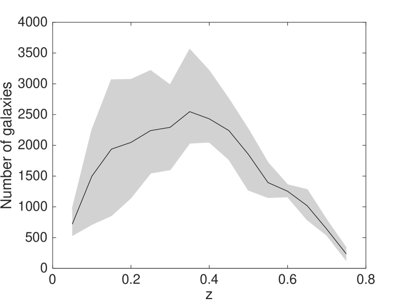
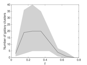
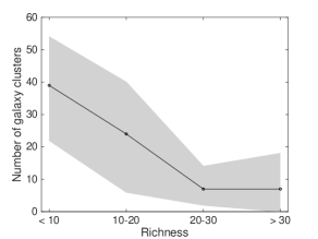
We tested the developed methods of determining the composition of the large scale galaxy distribution on 10 MICE collaboration [21] data sets from lightcone body simulation. All galaxy samples are restricted by an area of 2 square degrees, a limiting magnitude of and redshift from to , which corresponds to the limitations of the observed data which will be analyzed in the future. The coordinates on the sample field centers, as well as the number of galaxies and their clusters for each of the 10 data sets are presented in the Table. We also constructed plots of the distribution of the number of galaxies as a function of redshift (Fig. 1) and the distribution of the number of galaxy clusters as a function of redshift and cluster richness (Fig. 2). The plots demonstrate a rapid increase in the number of galaxies and clusters at – and a decrease at –, determined by the threshold magnitude of the samples. The majority of the galaxies which are related to large scale structures are collected into groups in the studied samples, and only a few are related to clusters.
The data of the MICECAT mock catalog are convenient for testing algorithms of large scale structure selection, since they contain information on the dark matter halo which a galaxy belongs to. Correspondingly, galaxies with the same halo identifier belong to the same cluster and are gravitationally bound.
Since the methods of analysis were developed for subsequent work with the data obtained with the 1-m Schmidt telescope of BAO NAS, the accuracy of photometric redshift determination for which is , candidates to various structures were determined for narrow layers of the large scale structure with a step of for all methods; we also added to this interval 25% of its value on each side, in order to avoid losses in determining galaxy clusters that are positioned on the boundary between the two layers.
2.1 Algorithm of Determining the Density Contrast with Adaptive Kernel


The galaxy distribution density was determined in the neighborhood of each considered galaxy as:
| (1) |
The size of the area , or the adaptive kernel which was used to smooth the galaxy density, was determined by the distance from the galaxy to the -th nearest neighbor as a three dimensional distance between the -th galaxy and its -th neighbor [26]:
| (2) |
where the Cartesian coordinates are computed by the formulas of conversion from spherical to Cartesian coordinate systems:
| (3) | |||
The angles , (in radians); —scaling factor, —redshift of the -th galaxy; —the comoving distance of the -th galaxy is calculated according to the formula from [27]:
| (4) |
Clusters and groups of galaxies are defined as peaks on density contrast maps of the distribution of galaxies. To mark the positions of the density peaks we determine the average density in a slice
| (5) |
Here is the number of galaxies in each slice. We then compute the value showing the density contrast in each point and interpolate the density contrast values over the entire field.
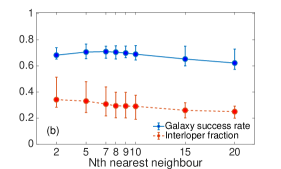
In this work we investigated the use of adaptive apertures up to the 2nd, 5th, 7th, 8th, 10th and 20th neighbor (Fig. 3). Statistical estimates (see Section 2.4) show that increasing the size of the adaptive kernel leads to the blurring of peaks on density contrast maps of the galaxy distribution and to the under-estimation of the large scale structures. We selected the distance to the 8th neighbor as a operating aperture of the method, which best allows us to isolate various structures.
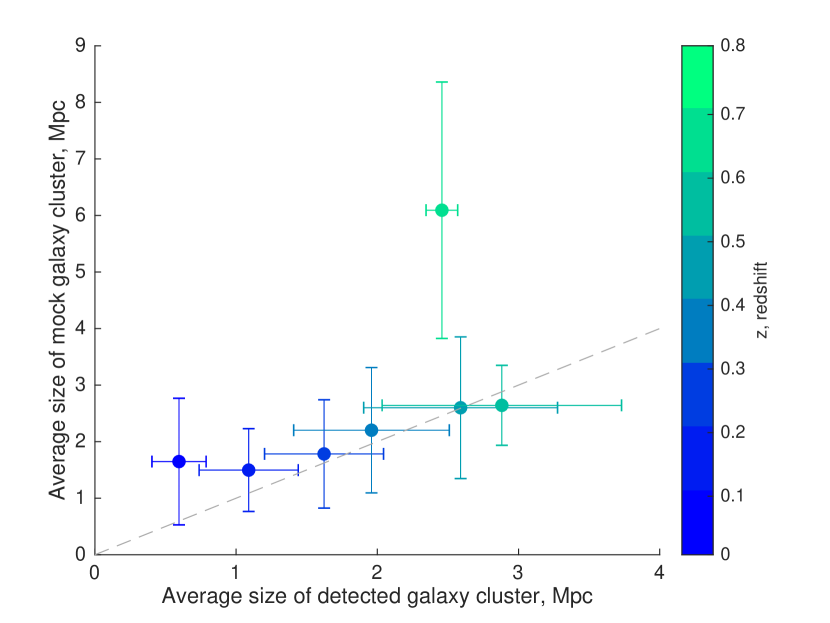
For the operating aperture we also estimated the average sizes of the detected clusters depending on the average sizes of the clusters in the mock catalog in redshift slices (Fig. 4) corresponding to the current notions about the sizes of galaxy clusters from 2 to 5 Mpc. Only two clusters fall within the range of among the 10 MICE catalog samples, which explains the large data scatter in this point. For the galaxy clusters are absent in the catalog due to the limitations and the number of cluster members (more than eight); there are also no detected clusters there.
2.2 Voronoi Tesselation Algorithm for Determining the Density Contrast
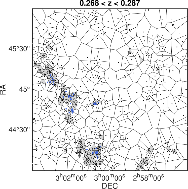
A Voronoi tesselation is defined as such a geometric devision of a plane into a polygon which possesses the following property: for any center of a system of points there is a region of space (polygon or Voronoi region) where all points are closer to the given center than to any other system center [28]. In this work, we use the considered galaxies as Voronoi region peaks. The procedure of dividing a two dimensional projection of a layer of the three dimensional large scale galaxy distribution was carried out with the procedures ‘voronoi’ and ‘voronoi’ in MatLab environment.
The inverse area of a Voronoi region is the numerical density corresponding to each galaxy—a polygon vertex. Groups and clusters of galaxies are determined in a way similar to the previous method, by the peaks on the density contrast map for the galaxy distribution field. The density contrast is defined as , and the average slice density:
| (6) |
where is the area of the Voronoi polygon around the -th galaxy, and is the number of Voronoi cells in the considered layer [29]. When computing the average density we do not take into account the boundary points for which the Voronoi cells tend to infinity.
2.3 Determining Groups and Clusters of Galaxies
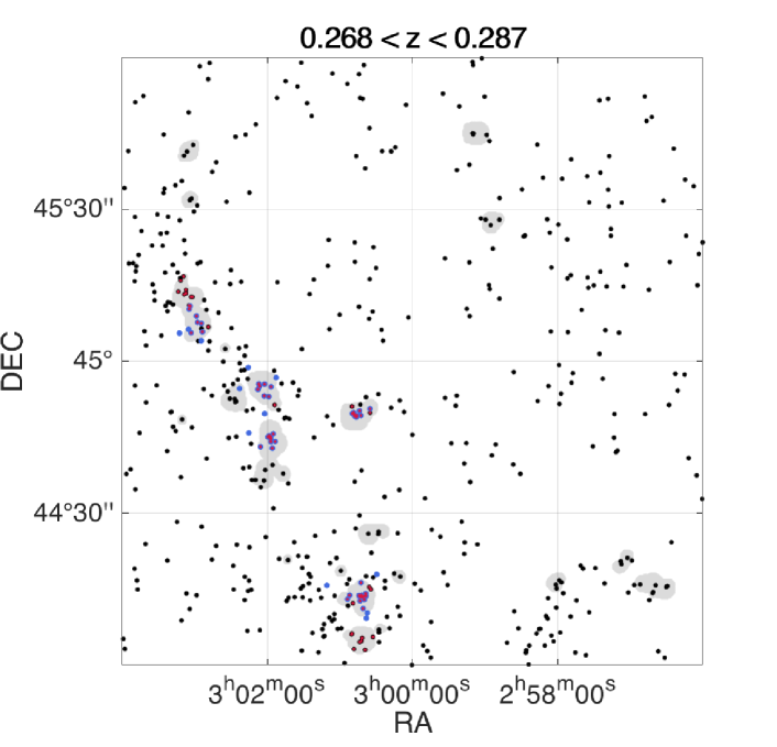
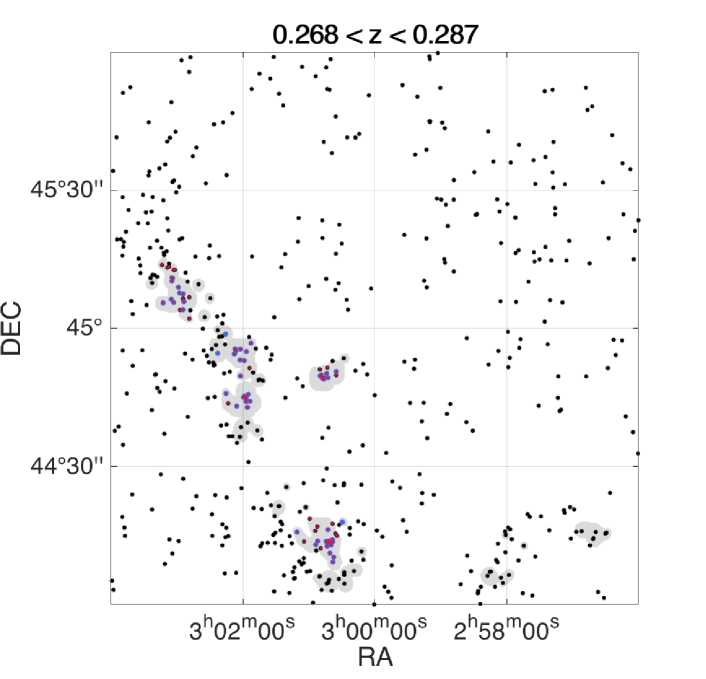
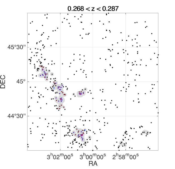
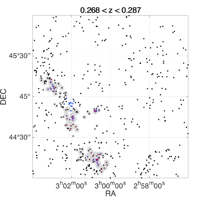
We selected regions with a density contrast of as galaxy group and cluster candidates. For the algorithm using adaptive kernel a galaxy group or cluster candidate must contain more than nine galaxy members inside the region with the density contrast greater than , and for the Voronoi algorithm it must fulfill the condition of at least eight other cells with a density contrast higher than located near the cell (see Section 2.4). An example of dividing a narrow slice of the large scale redshift distribution with marked detected clusters and clusters from the catalog is presented in Fig. 5.
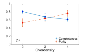
On the whole, both methods of analyzing the large scale distribution of galaxies give compatible results. However, the Voronoi tesselation method, despite the high fraction of detected cluster member galaxies and identified clusters in the catalogs in general, shows a much smaller sample purity both in terms of clusters and galaxies (see Fig. 6). We can thus conclude that the Voronoi tesselation method may be useful as an additional tool for identifying clusters, whereas the adaptive kernel algorithm should be used as the main instrument.
2.4 Basic Statistical Calculations
Since the MICE galaxy mock catalog has a parameter that determines the cluster membership of a galaxy, we can estimate the quality of the developed algorithms using statistical methods. We used the statistical estimation criteria from [30, 31]. According to these papers, group is considered to correspond to group if group contains more than of group galaxies. From this we can determine that the correspondence can be one sided when group corresponds to group and the reverse is false, and mutual when group corresponds to group and vice versa. In this work we assume that group corresponds to group if group contains more than of galaxies belonging to .
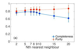
The terms of sample completeness and purity can also be defined for the one sided and two sided correspondence. Let us denote by the number of galaxy groups and clusters in the model catalog, and let represent the number of groups and galaxies determined by the program algorithms. Then the “one-sided sample completeness” of the clusters corresponding to the dark matter halo of the model catalog clusters is computed as
| (7) |
where is the number of matches between the real groups from the catalog and the groups determined automatically.
The “two-sided sample completeness”:
| (8) |
here is the number of matches of real groups from the catalog and groups determined automatically and vice versa. The purity of the sample can be determined in a similar way:
| (9) |
| (10) |
The four quantities can take only values between and . A close to value of parameter shows that the number of undefined groups in the catalogs is small. For parameter such a value shows a small fraction of falsely detected clusters. The to and to ratios close to zero show an overestimation (one automatically detected group corresponds to several groups in the catalog) or fragmentation (one catalog group corresponds to several automatically identified groups) of the groups.
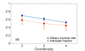
The statistical parameters , , and characterize the work of program algorithms for groups and clusters of galaxies. In order to estimate it for the galaxies in groups, let us denote the sample of galaxies in groups and clusters in the model catalog as , and the sample of galaxies in the automatically identified clusters as . We then introduce a parameter that shows the fraction of successfully determined galaxies from the mock catalog:
| (11) |
The denominator in this expression is equal to the number of the same members in samples and . This parameter shows what fraction of galaxies in groups and clusters of the mock catalog were identified automatically.
The second parameter characterizing the work of the program algorithms for galaxies is the interloper fraction. This is the fraction of all galaxies that were automatically grouped into clusters, but which are field galaxies in the model catalog.
| (12) |
Parameters and will also take values between and .
Evidently, it is impossible to have an ideal match between the model catalog and the reconstructed groups and clusters. However, we can optimize the work of the algorithms based on the parameters presented above, using the quality parameters for the obtained samples, determined as follows:
| (13) |
| (14) |
| (15) |
The parameter shows the balance between the completeness and purity parameters of the derived sets of galaxy groups and clusters, parameter —that between the one-sided and two-sided correspondence, and parameter is similar to , but, unlike , which characterizes the detection of galaxy groups with respect to the groups in the catalog, it shows the relation between individual detected galaxies and groups. All three parameters can take only values between and . When comparing the statistical parameters for the derived sets of detected groups, one must try to minimize the parameters and , and maximize the parameter .
Since the filtering method with adaptive kernel has the option to vary its size, we computed for each of the considered apertures the corresponding parameters of the detected cluster sample quality in order to optimize the work of the algorithm. The best parameters were obtained for the adaptive kernel size . This size was selected as optimal for further investigations.
For the Voronoi tesselation method, there are no parameters similar to the method of adaptive kernel, which could be varied within the algorithm. However, we can use different density contrast values, which determine the membership of galaxies in groups and clusters. The optimal density contrast based on the quality parameters for the obtained group and cluster samples has a value of two.
3 VOID IDENTIFICATION
Isolating spatial regions of low density may also be useful for further investigations based on the observed data for the physical properties of galaxies as functions of the surrounding density. The results obtained during the previous stage (density contrast values for the galaxies of the large scale distribution) can be used to determine galaxies located in voids. According to modern notions, the density contrast of void galaxies is an order of magnitude less than the average density of the distribution of galaxies [12].
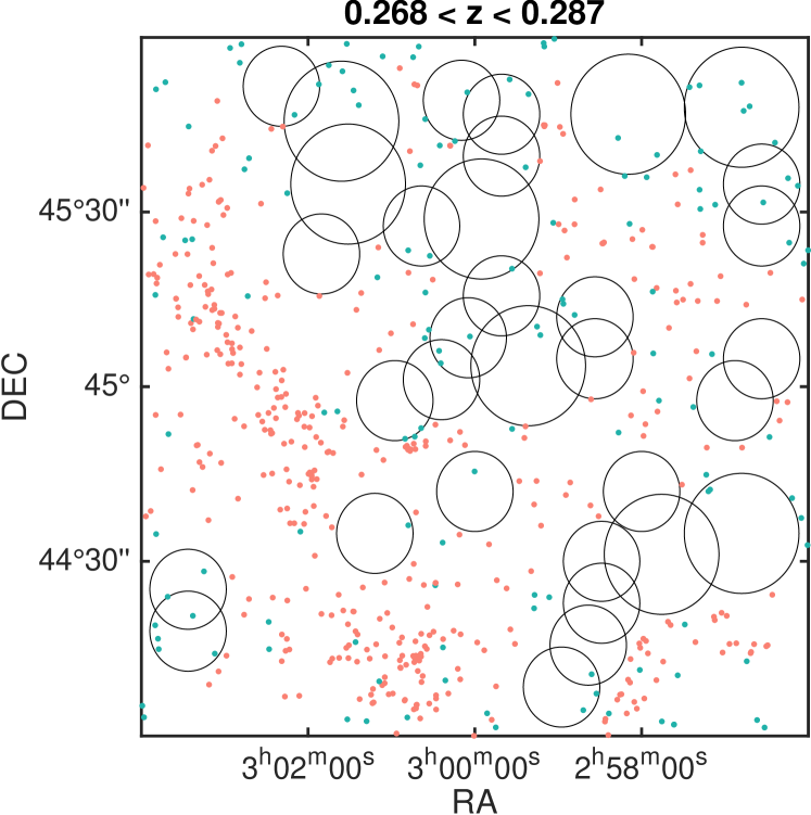
The method used by us to determine voids is based on the algorithm presented in [32] for statistical void analysis from the 2dFGRS [5] survey. For determining voids in each layer we used a grid of points, which was superimposed onto each layer separately. For each point we determined circles of maximum diameter within which there are either no galaxies at all, or only galaxies for which we determined in the previous step that the density of their surroundings is one order of magnitude smaller than the average density in the layer. The voids were restricted from one side by the field boundaries, from the other —by galaxies for which the surrounding density was greater than the density of the void galaxies. The step of the circle radii variation was selected as radians, which corresponds to a value from to Mpc depending from redshift. The step size of the variation was chosen based on the optimal computing time for close and distant redshifts.
We then selected the void-circles in such a way that the centers of the selected circles should not lie within other identified circles, and have the maximum radius among all those possible for the given layer region. Additionally, with the redshift increase, we imposed a restriction on the minimal volume of the detected void.
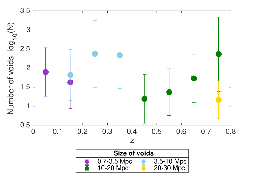
An example of detecting voids for a thin slice of the three dimensional galaxy distribution is presented in Fig. 7. During the course of studying the work of the algorithm for 10 sets of data from the MICE simulation we discovered that the voids rarely have spherical shape, being united into various structures (chains, etc.). For the mock data of the MICE simulation we estimated the average sizes of the identified voids and their number (Fig. 8) as a function of redshift. As is evident from the plot, mini-voids with sizes of approximately – Mpc are dominant at the redshift –, and with an increase in the size of the field we are able to detect voids with an average size of about – Mpc.
4 CONCLUSIONS
We developed algorithms of multiparameter analysis of the large scale distribution of galaxies in narrow slices in the entire range of redshifts, including methods of determining clusters and groups of galaxies by constructing density contrast maps, and also determining voids. The results of using these algorithms correspond to the visual estimate of the structures in slices, and the average sizes of the detected clusters and voids correspond to the current estimates with account of the size of the considered field. A numerical estimation of the results of the methods of density contrast map construction and identification of groups and clusters was made for 10 data sets for galaxies and their clusters from the MICE simulation, which allowed us to estimate the completeness and purity of the sample, and also the fraction of correctly identified galaxies as well as galaxies which were misclassified as cluster galaxies. We can conclude that the developed algorithms are a stable method of determining galaxy group and cluster candidates as well as intergalactic void candidates.
The method presented in this work will be used in the future to study the large scale distribution of galaxies using the observed data obtained with the 1 meter Schmidt telescope of the Byurakan astrophysical observatory, and also to investigate the influence of the surroundings on the physical properties of galaxies (mass, luminosity, star formation rate).
5 ACKNOWLEDGMENTS
The authors are grateful to the referee for constructive feedback on the initial text of the paper. This work has made use of CosmoHub. CosmoHub has been developed by the Port d’Informacio Cientifica (PIC), maintained through a collaboration of the Institut de Fisica d’Altes Energies (IFAE) and the Centro de Investigaciones Energeticas, Medioambientales y Tecnologicas (CIEMAT), and was partially funded by the “Plan Estatal de Investigacion Cientifica y Tecnica y de Innovacion” program of the Spanish government.
FUNDING
This work was carried out with the financial support of the Russian Science Foundation, project 17-12-01335 “Ionized gas in galactic discs and beyond the optical radius”.
CONFLICT OF INTEREST
The authors declare no conflict of interest.
References
- [1] E. P. Hubble, ApJ 64, 321 (1926).
- [2] M. Fioc and B. Rocca-Volmerange, Astronomy and Astrophysics 351, 869 (1999).
- [3] A. Oemler, PhD Thesis (California Institute of Technology, 1974).
- [4] A. Dressler, ApJ 236, 351 (1980).
- [5] D. S. Madgwick, E. Hawkins, O. Lahav, et al., MNRAS 344, 847 (2003).
- [6] H. Guo, I. Zehavi, Z. Zheng, et al., ApJ 767, 122 (2013).
- [7] H. Guo, Z. Zheng, I. Zehavi, et al., MNRAS 441, 2398 (2014).
- [8] G. Kauffmann, S. D. M. White, T. M. Heckman, et al., MNRAS 353, 713 (2004).
- [9] O. Cucciati, A. Iovino, K. Kovac, et al., Astronomy and Astrophysics 524, A2 (2010).
- [10] G. De Lucia, B. M. Poggianti, A. Aragon-Salamanca, et al., IAU Colloquium 195, 473 (2004).
- [11] O. Cucciati, A. Iovino, C. Marinoni, et al., Astronomy and Astrophysics 458, 39 (2006).
- [12] R. van de Weygaert and E. Platen, International Journal of Modern Physics: Conference Series 1, 41 (2011).
- [13] A. K. Romer, P. T. P. Viana, A. R. Liddle, and R. G. Mann, ApJ 547, 594 (2001).
- [14] M. Pierre, F. Pacaud, P. A. Duc, et al., MNRAS 372, 591 (2006).
- [15] A. Finoguenov, L. Guzzo, G. Hasinger, et al., ApJS 172, 182 (2007).
- [16] J. E. Carlstrom, G. P. Holder, and E. D. Reese, Annual Review of Astronomy and Astrophysics 40, 643 (2002).
- [17] G. M. Voit, Reviews of Modern Physics 77, 207 (2005).
- [18] N. N. Weinberg and M. Kamionkowski, MNRAS 337, 1269 (2002).
- [19] P. A. A. Lopes, R. R. de Carvalho, R. R. Gal, et al., AJ 128, 1017 (2004).
- [20] B. P. Koester, T. A. McKay, J. Annis, et al., ApJ 660, 221 (2007).
- [21] J. Carretero, P. Tallada, J. Casals, et al., in Proc. of the European Physical Society Conference on High Energy Physics (Venice, 2017), p. 488.
- [22] G. O. Abell, ApJS 3, 211 (1958).
- [23] F. Zwicky, E. Herzog, P. Wild, et al., Catalogue of galaxies and of clusters of galaxies, Vol. I (California Institute of Technology, Pasadena, 1961).
- [24] S. A. Shectman, ApJS 57, 77 (1985).
- [25] R. J. Dodd and H. T. MacGillivray, AJ 92, 706 (1986).
- [26] T. W. B. Kibble and F. H. Berkshire, Classical Mechanics (5TH Edition) (World Scientific Press, 2004).
- [27] J. A. Peacock, Cosmological Physics (Cambridge University Press, Cambridge, 1999).
- [28] M. Ramella, W. Boschin, D. Fadda, and M. Nonino, Astronomy and Astrophysics 368, 776 (2001).
- [29] I. K. Sochting, G. V. Coldwell, R. G. Clowes, et al., MNRAS 423, 2436 (2012).
- [30] B. F. Gerke, J. A. Newman, M. Davis, et al., ApJ 625, 6 (2005).
- [31] C. Knobel, S. J. Lilly, A. Iovino, et al., ApJ 697, 1842 (2009).
- [32] S. G. Patiri, J. E. Betancort-Rijo, F. Prada, et al., MNRAS 369, 335 (2006).