A Dynamical Survey of Stellar-Mass Black Holes in 50 Milky Way Globular Clusters

Abstract

Recent numerical simulations of globular clusters (GCs) have shown that stellar-mass black holes (BHs) play a fundamental role in driving cluster evolution and shaping their present-day structure. Rapidly mass-segregating to the center of GCs, BHs act as a dynamical energy source via repeated super-elastic scattering, delaying onset of core collapse and limiting mass segregation for visible stars. While recent discoveries of BH candidates in Galactic and extragalactic GCs have further piqued interest in BH-mediated cluster dynamics, numerical models show that even if significant BH populations remain in today’s GCs, they are not typically in directly detectable configurations. We demonstrated in Weatherford et al. (2018) that an anti-correlation between a suitable measure of mass segregation ($\Delta$) in observable stellar populations and the number of retained BHs in GC models can be applied to indirectly probe BH populations in real GCs. Here, we estimate the number and total mass of BHs in 50 Milky Way GCs from the ACS Globular Cluster Survey. For each GC, $\Delta$ is measured between observed main sequence populations and fed into correlations between $\Delta$ and BH retention found in our CMC Cluster Catalog’s models. We demonstrate the range in measured $\Delta$ from our models matches that for observed GCs to a remarkable degree. Our results constitute the largest sample of GCs for which BH populations have been predicted to-date using a self-consistent and robust statistical approach. We identify NGCs 2808, 5927, 5986, 6101, and 6205 to retain especially large BH populations, each with total BH mass exceeding $10^{3}\,{\rm{M_{\odot}}}$.

1 Introduction

Our understanding of stellar-mass black hole (BH) populations in globular clusters (GCs) has rapidly improved since the turn of the century. To date, five BH candidates have been detected in Milky Way GCs via X-ray and radio observations: two in M 22 (Strader et al., 2012), plus one each in M 62 (Chomiuk et al., 2013), 47 Tuc (Miller-Jones et al., 2015; Bahramian et al., 2017), and M 10 (Shishkovsky et al., 2018). More recently, three BHs in detached binaries have been reported in NGC 3201, the first to be identified using radial velocity measurements (Giesers et al., 2018, 2019). Additional candidates have been spotted in extragalactic GCs (e.g., Maccarone et al., 2007; Irwin et al., 2010). The lack of any particular pattern in the GCs hosting BH candidates suggests that perhaps most GCs in the Milky Way (MWGCs) retain BH populations to present.

Such observational evidence complements a number of recent computational simulations which show that realistic clusters can retain up to thousands of BHs late in their lifetimes (e.g., Morscher et al., 2015). It is now clear that BH populations play a significant role in driving long-term cluster evolution and shaping the present-day structure of GCs (Merritt et al., 2004; Mackey et al., 2007, 2008; Breen & Heggie, 2013; Peuten et al., 2016; Wang et al., 2016; Chatterjee et al., 2017b, a; Weatherford et al., 2018; Arca Sedda et al., 2018; Kremer et al., 2018b; Zocchi et al., 2019; Kremer et al., 2019; Antonini & Gieles, 2020; Kremer et al., 2020).

The dynamical importance of BHs in GCs is reflected in their ability to explain the bimodal distribution in core radii distinguishing so-called ‘core-collapsed’ clusters from non-core-collapsed clusters. A convincing explanation for this bimodality, specifically why most GCs are not core-collapsed despite their short relaxation times, has challenged stellar dynamicists for decades. However, recent work by Kremer et al. (2019, 2020) has shown that cluster models naturally reproduce the range of observed cluster properties (such as core radius) when their initial size is varied within a narrow range consistent with the measured radii of young clusters in the local universe (Portegies Zwart et al., 2010). The missing piece in the explanation is simply the BHs, which guide a young cluster’s evolution to manifest present-day structural features. In this picture, most clusters retain a dynamically-significant number of BHs to the present. As the BHs mass-segregate to the cluster core, they provide enough energy to passing stars in scattering interactions (via two body relaxation) to support the cluster against gravothermal collapse, at least until their ejection from the cluster (Mackey et al., 2008). For an in-depth discussion of this ‘BH burning’ process, see Breen & Heggie (2013); Kremer et al. (2020). Clusters born with high central densities rapidly extract the BH-driven dynamical energy, ejecting nearly all BHs by the present. With the ensuing reduction in dynamical energy through BH burning, the BH-poor clusters swiftly contract to the observed core-collapsed state.

Despite these advances to our understanding of BH dynamics among the cluster modeling community, observationally inferring the presence of a stellar-mass BH subsystem (BHS) in the core of a GC remains difficult. Contrary to expectations, results from $N$-body simulations suggest that the number of mass-transferring BH binaries in a GC does not correlate with the total number of BHs in the GC at the time (Chatterjee et al., 2017b; Kremer et al., 2018a). Since the majority of BH candidates in GCs come from this mass-transferring channel, the observations to-date are of little use in constraining the overall number and mass of BHs remaining in clusters. Several groups have suggested that the existence of a BHS in a GC can be indirectly inferred from structural features, such as a large core radius and low central density (e.g., Merritt et al., 2004; Hurley, 2007; Morscher et al., 2015; Chatterjee et al., 2017b; Askar et al., 2017b; Arca Sedda et al., 2018). However, interpretation of such features is ambiguous; the cluster could be puffy due to BH dynamics-mediated energy production or simply because it was born puffy (equivalently, with a long initial relaxation time). Others have suggested that radial variation in the present-day stellar mass function slope may reveal the presence of a BHS (e.g., Webb & Vesperini, 2016; Webb et al., 2017). The challenge here is that obtaining enough coverage of a real GC to measure its mass function over a wide range in radial position requires consolidating observations from different space- and ground-based instruments.

Due to the above ambiguities in interpreting a GC’s large-scale structural features and observational difficulties in finding its mass-function slope, we recently introduced a new approach to predict the BH content in GCs using mass segregation among visible stars from different mass ranges (Weatherford et al., 2018, W1 hereafter). In a journey towards energy equipartition, heavier objects in a cluster give kinetic energy to passing lighter objects through scattering interactions (two body relaxation), eventually depositing the most massive objects (the BHs) at the center, with increasingly lighter stars distributed further and further away, on average (e.g., Binney & Tremaine, 1987; Heggie & Hut, 2003). The most massive stars mass-segregate closest to the central BH population, thereby undergoing closer and more frequent scattering interactions with the BHs than do less massive stars distributed further away. While BH burning drives all non-BHs away from the cluster center, the heavier objects receive proportionally more energy through this process. So, increasing the number (total mass) of BHs decreases the radial ‘gap’ between the distributions of higher-mass and lower-mass stars. The presence of a central BH population thereby quenches mass segregation (e.g., Mackey et al., 2008; Alessandrini et al., 2016), an effect we can quantify by comparing the relative locations of stars from different mass ranges.

Low levels of mass segregation were first used to infer the existence of an intermediate-mass BH (IMBH) at the center of a GC over a decade ago (Baumgardt et al., 2004; Trenti et al., 2007). More recently, Pasquato et al. (2016) used such a measure to place upper limits on the mass of potential IMBHs in MWGCs. Peuten et al. (2016) further suggested the lack of mass segregation between blue stragglers and stars near the main sequence turnoff in NGC 6101 may be due to an undetected BH population. W1, however, was the first study to use mass segregation to predict the number of stellar-mass BHs retained in specific MWGCs (47 Tuc, M 10, and M 22). In this study, we improve upon the method first presented in W1 and apply it to predict the number (${N_{\rm{BH}}}$) and total mass (${M_{\rm{BH}}}$) of stellar-mass BH populations in 50 MWGCs from the ACS Globular Cluster Survey (Sarajedini et al., 2007).

We describe our models and how they are ‘observed’ in Section 2. In Section 3, we define the stellar populations used to quantify mass segregation ($\Delta$), describe how we measure $\Delta$ in MWGCs from the ACS Globular Cluster Survey, and detail the steps necessary to accurately compare $\Delta$ measured in our models to $\Delta$ measured in observed clusters. We present our own present-day ${N_{\rm{BH}}}$ and ${M_{\rm{BH}}}$ predictions for 50 MWGCs in Section 4, discuss how they support our BH burning model in Section 5, and finally compare the predictions to previous results (most notably from the MOCCA collaboration) in Section 6. Finally, in Section 7, we summarize all key findings and discuss a few potential wider interpretations of our results regarding primordial mass segregation and IMBHs hosted in MWGCs.

2 Numerical Models

In this paper, we use the large grid of 148 cluster simulations presented in the CMC Cluster Catalog (Kremer et al., 2020), computed using the latest version of our Hénon-type (Hénon, 1971a, b) Cluster Monte Carlo code (CMC). CMC has been developed and rigorously tested over the last two decades (Joshi et al., 2000, 2001; Fregeau et al., 2003; Fregeau & Rasio, 2007; Chatterjee et al., 2010; Umbreit et al., 2012; Pattabiraman et al., 2013; Chatterjee et al., 2013). For the most recent updates and validation of CMC see Morscher et al. (2015); Rodriguez et al. (2016, 2018); Kremer et al. (2020).

As described by Kremer et al. (2020), the grid covers roughly the full parameter space spanned by the MWGCs, with the range of variations motivated by observational constraints from high-mass young star clusters, thought to be similar in properties to GC progenitors (e.g., Scheepmaker et al., 2007; Chatterjee et al., 2010). We vary four initial parameters: the total number of particles ($N=2\times 10^{5}$, $4\times 10^{5}$, $8\times 10^{5}$, and $1.6\times 10^{6}$), the cluster virial radius ($r_{v}/{\rm{pc}}=0.5,\,1,\,2,\,4$), the metallicity (${\rm{Z}}/{\rm{Z}}_{\odot}=0.01,\,0.1,\,1$), and the Galactocentric distance ($R_{\rm{gc}}/{\rm{kpc}}=2,\,8,\,20$) assuming a Milky Way-like galactic potential (e.g., Dehnen & Binney, 1998). This yields a $4\times 4\times 3\times 3$ grid of 144 simulations. We also run four additional simulations with $N=3.2\times 10^{6}$ particles to characterize the most massive MWGCs. For these, we fix the Galactocentric distance to $R_{\rm{gc}}/{\rm{kpc}}=20$ while varying metallicity (${\rm{Z}}/{\rm{Z}}_{\odot}=0.01,\,1$) and virial radius ($r_{v}/{\rm{pc}}=1,\,2$). Finally, note that we exclude a handful of simulations which disrupted before reaching $13\,{\rm{Gyr}}$ in age (described in Kremer et al., 2020) to ensure that our results are not affected by clusters close to disruption – at that point, the assumption of spherical symmetry in CMC is incorrect. In total, we use $118$ simulations, each with a unique combination of initial properties.

In all simulations, the positions and velocities of single stars and centers of mass of binaries are drawn from a King profile with concentration $w_{0}=5$ (King, 1966). Stellar masses (primary mass in case of a binary) are drawn from the initial mass function (IMF) given in Kroupa (2001) between $0.08$ and $150\,{\rm{M_{\odot}}}$. Binaries are assigned by randomly choosing $N\times f_{b}$ stars independent of radial position and mass and assigning a secondary adopting a uniform mass ratio ($q$) between $0.08/m_{p}$ and $1$, where $m_{p}$ denotes the primary mass and the binary fraction is set to $f_{b}=0.05$ in all models. Binary orbital periods are drawn from a distribution flat in log scale with bounds from near contact to the hard-soft boundary. Binary eccentricities are drawn from a thermal distribution. We include all relevant physical processes, such as two body relaxation, strong binary-mediated scattering, and galactic tides using the prescriptions outlined in Kremer et al. (2020).

Single and binary stellar evolution are followed using the SSE and BSE packages (Hurley et al., 2000, 2002), updated to include our latest understanding of stellar winds (e.g., Vink et al., 2001; Belczynski et al., 2010) and BH formation physics (e.g., Belczynski et al., 2002; Fryer et al., 2012). Neutron stars (NS) receive natal kicks drawn from a Maxwellian with $\sigma=265\,{\rm{km\,s^{-1}}}$. The maximum NS mass is fixed at $3\,{\rm{M_{\odot}}}$; any remnant above this mass is considered a BH. The BH mass spectrum depends on the metallicities and pre-collapse mass (Fryer et al., 2012). BH natal kicks are based on results from Belczynski et al. (2002); Fryer et al. (2012). Namely, a velocity is first drawn from a Maxwellian with $\sigma=265\,{\rm{km\,s^{-1}}}$, then scaled down based on the metallicity-dependent fallback of mass ejected due to supernova. These prescriptions lead to $\sim 10^{-3}N$ retention of BHs immediately after they form. By the late times of interest ($t\geq 9\,{\rm{Gyr}}$), our simulated clusters retain a median of 3% (0–17%) and 2% (0–32%) of the total formed NSs and BHs, respectively. More detailed descriptions and justifications are given in past work (e.g., Morscher et al., 2015; Wang et al., 2016; Askar et al., 2017b). However, note that the primary results in this work do not depend on the exact prescriptions for BH natal kicks, provided that a dynamically significant BH population remains in the cluster post-supernova. These results are expected to depend indirectly on the BH birth mass function, via modest differences it may create in the cluster’s average stellar mass at late times.

2.1 ‘Observing’ Model Clusters

CMC periodically outputs dynamical and stellar properties of all single and binary stars including the luminosity ($L$), temperature ($T$), and radial positions. Assuming spherical symmetry, we project the radial positions of all single and binary stars in two dimensions to create sky-projected snapshots of simulations at different times. In line with the typical age range of MWGCs, we use all snapshots ($7,355$ total or $\sim 60$ per simulation) corresponding to ages between $9$ and $13\,{\rm{Gyr}}$.

For each single star we calculate the temperature $T$ from the luminosity $L$ and the stellar radius $R$ (given by BSE) assuming a blackbody. We treat binaries as unresolved sources, assigning the combined luminosity $L=L_{1}+L_{2}$ and an effective temperature given by the $L$-weighted mean (Eq. 1; W1).

To account for statistical fluctuations, we project each snapshot in two dimensions assuming ten random viewing angles. For each 2D projection, we then calculate the core radius (${r_{c,\rm{obs}}}$) and central surface luminosity density (${\Sigma_{c,\rm{obs}}}$) by fitting an analytic approximation of the King model (Eq. 18; King, 1962) to the cumulative luminosity profile (e.g., Chatterjee et al., 2017b). We also calculate the half-light radius (${r_{\rm{hl}}}$) as the sky-projected distance from the center within which half of the total cluster light is emitted.

3 Mass Segregation in Models and Observed Clusters

In general, quantifying $\Delta$ in a star cluster requires comparing the radial distributions of multiple stellar populations sufficiently different in their average masses (e.g., Goldsbury et al., 2013). While stellar mass is not directly measured in real clusters, stellar luminosity is, and can be used as a proxy for mass, especially for main sequence (MS) stars (e.g., Hansen & Kawaler, 1994). As in W1, we anchor our population definitions to the location of the MS turnoff (MSTO), the most prominent feature on a color-magnitude or Hertzsprung-Russel diagram (Figure 1). Defining the MSTO at $L={L_{\rm{TO}}}$, where the MS stars (excluding blue stragglers) exhibit the highest temperature, population bounds are then established as fractions of ${L_{\rm{TO}}}$. While these details are unchanged from W1, we have upgraded the specific population choices used to measure $\Delta$.

In W1, we sought to maximize the signal strength in $\Delta$ by choosing two populations with characteristic masses (luminosities) as different as possible while still ensuring that the lighter population is bright enough to be easily observable in the MWGCs. In addition, both populations must contain large enough numbers of stars to limit statistical scatter. Under these constraints, we chose a high-mass population containing all stars with $L>{L_{\rm{TO}}}$ and a low-mass population consisting of MS stars with ${L_{\rm{TO}}}/125\leq L\leq{L_{\rm{TO}}}/25$. While these population choices (Pop1 and Pop4 in Figure 1) maximized the magnitude of $\Delta$ while ensuring relatively large observable population sizes, reducing statistical scatter compared to other choices in previous studies (e.g., blue stragglers; Peuten et al., 2016; Alessandrini et al., 2016), they were not free from drawbacks (de Vita et al., 2019). Specifically, Pop1 contains far fewer stars than any of the three MS populations, introducing higher statistical scatter than strictly necessary. Furthermore, an extreme luminosity difference between populations can cause them to suffer from large discrepancies in observational incompleteness, in which dim stars are washed out by bright neighbors. As shown in W1, difference in the radially-dependent incompleteness between populations can introduce significant uncertainty in the measured $\Delta$, and by extension, the inferred number of BHs.

For example, the median masses for Pop1 and Pop2 are $0.82\,{\rm{M_{\odot}}}$ and $0.75\,{\rm{M_{\odot}}}$, respectively, a minor gap (Figure 1). Meanwhile, the stellar luminosity in Pop1 spans nearly 3 orders of magnitude. Independent of our choice for the other population, Pop1’s inclusion in the $\Delta$ calculation balloons the incompleteness difference between populations, resulting in increased uncertainty. In contrast, the three MS populations (Pop2, Pop3, Pop4) differ much more significantly in their median mass with comparatively small variation in their typical luminosities. In this work, we therefore use only these MS populations to compute $\Delta$ and ignore Pop1.

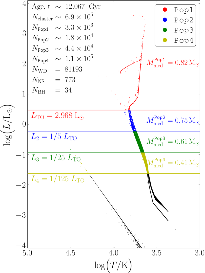
Figure 1: Example Hertzsprung-Russell diagram showing the four stellar populations used to measure mass segregation in a typical CMC model at $12\,{\rm{Gyr}}$ ($N=8\times 10^{5}$, $r_{v}=1\,{\rm{pc}}$, $R_{\rm{gc}}=8\,{\rm{kpc}}$, and ${\rm{Z}}=0.01\,{\rm{Z}}_{\odot}$). Each data point represents a single or binary star (all binaries are considered unresolved). The highest-mass population (Pop1, in red) encompasses all stars above the MS turnoff (delineated in red), which is defined as the luminosity corresponding to the highest temperature on the MS (excluding blue stragglers). The three lower-mass populations (Pop2 in blue, Pop3 in green, and Pop4 in yellow) are evenly spaced in log scale along the MS with lower boundaries delineated in the corresponding colors. The median masses for all populations are shown in the figure. Relevant cluster properties at the time of this snapshot such as $N$, ${N_{\rm{BH}}}$, and the respective numbers in each stellar population are also included. Defining stellar populations this way ensures a high number of stars in each population, with highest sample sizes for dimmer populations.

3.1 Quantifying Mass Segregation

Having chosen three distinct MS populations, we compute the mass segregation, $\Delta$, between any pair of them using both parameters introduced in W1. The first, ${\Delta_{r50}}^{ij}$, is the difference in median cluster-centric distance between ${\tt{Pop}}i$ and ${\tt{Pop}}j$. The second, ${\Delta_{A}}^{ij}$ is the difference in area under the two populations’ cumulative radial distributions. In both cases, the cluster-centric radial distances used are sky-projected and normalized by the cluster’s sky-projected half-light radius to make $\Delta$ unitless. Mathematical expressions and graphical representations of these mass segregation parameters are given in Section 2.3 of W1.

3.2 $\Delta$ vs ${N_{\rm{BH}}}/{N_{\rm{cluster}}}$ (${M_{\rm{BH}}}/{M_{\rm{cluster}}}$) in models: Effects of cluster properties

As introduced in W1, there exists a strong anti-correlation between the ratio of BHs to total stars retained in a cluster (${N_{\rm{BH}}}$/${N_{\rm{cluster}}}$) and the cluster’s measured mass segregation (${\Delta_{r50}}^{ij}$ and ${\Delta_{A}}^{ij}$). The anti-correlation is due to BH burning, in which BHs mass-segregate to the core and provide energy to passing stars via two body relaxation, pushing those stars farther out into the cluster. On average, the most massive stars gain proportionally more energy since they are distributed closer to the BH-core than less massive stars. Hence, clusters with more numerous (more massive) BH populations in their core display reduced mass segregation.

In Figure 2, we show the $\Delta$-${N_{\rm{BH}}}/{N_{\rm{cluster}}}$ anti-correlation across all $7,355$ model snapshots with ages between $9$-$13\,{\rm{Gyr}}$, colored by metallicity and using a standard radial limit of ${r_{\rm{lim}}}={r_{\rm{hl}}}$. (i.e. Only stars within the model clusters’ half-light radii are used when measuring $\Delta$ for this figure, a constraint motivated by field-of-view limits when observing real clusters; see Section 3.3). In the top panel, ${\Delta_{r50}}^{24}$ (${\Delta_{r50}}$ between Pop2 and Pop4) is used for $\Delta$, while the lower panel uses ${\Delta_{A}}^{24}$. Uncertainty bars represent the standard deviation across the 10 randomized 2D projections (‘views’) of each cluster snapshot.

Though not shown, plots of ${M_{\rm{BH}}}/{M_{\rm{cluster}}}$ versus $\Delta$ are practically indistinguishable from Figure 2, except with a y-axis range of $\log({M_{\rm{BH}}}/{M_{\rm{cluster}}})\in[-1.3,-5.3]$. Other pairings of the four populations in Figure 1 to measure $\Delta$ also result in very similar anti-correlations, though wider spread is indeed apparent whenever Pop1 is used, for the reasons discussed earlier.

With both more models and much fuller coverage of the space of initial cluster parameters characterizing observed MWGCs ($N$, $r_{v}$, ${\rm{Z}}$, and $R_{\rm{gc}}$), the anti-correlation extends to larger mass segregation and to an order-of-magnitude lower ${N_{\rm{BH}}}/{N_{\rm{cluster}}}$ than in W1. The metallicity dependence of the trend is also more explicit. The higher the ${\rm{Z}}$, the lower the mass of the BHs produced, so higher-${\rm{Z}}$ clusters need higher ${N_{\rm{BH}}}/{N_{\rm{cluster}}}$ to quench $\Delta$ to the same degree as a lower-${\rm{Z}}$ cluster.

Other parameters contribute less visibly to the spread in the trend, primarily through their impact on dynamical age, which increases from upper left to lower right along the trend. Specifically, a detailed model-to-model examination reveals that virial radius ($r_{v}$) has the largest impact on a snapshot’s location along the trend at any given physical time. Clusters with lower initial $r_{v}$ relax faster, making them dynamically older at late times than GCs with higher $r_{v}$. Since $\Delta$ correlates with and ${N_{\rm{BH}}}$ anti-correlates with dynamical age, the models with lowest $r_{v}$ appear at the bottom right of each panel in Figure 2. Initial $N$ also affects the relaxation timescale of a cluster. Thus, the least massive clusters are also dynamically the oldest at the same physical time. These low-mass clusters tend to be at the bottom right. Similarly, all else being fixed, as a cluster gets older, it moves down and right along the trend, albeit to a lesser degree than movement from $N$ or $r_{v}$ variation, since the age range used here is narrow ($9$-$13\,{\rm{Gyr}}$) compared to lifetimes of typical GCs. For an average model, ${N_{\rm{BH}}}/{N_{\rm{cluster}}}$ drops by 0.5 dex between the $9$ and $13\,{\rm{Gyr}}$ snapshots. Finally, increasing Galactocentric distance ($R_{\rm{gc}}$) slightly increases $\Delta$ but has little impact on ${N_{\rm{BH}}}/{N_{\rm{cluster}}}$, shifting snapshots left-to-right in the figure. This occurs because clusters farther from the Galactic center experience lower tidal forces, increasing the cluster’s tidal radius (boundary) and making it harder for stars to escape the cluster. As will be discussed in the next section, limiting the radial extent of the stellar populations used to measure $\Delta$ decreases $\Delta$.

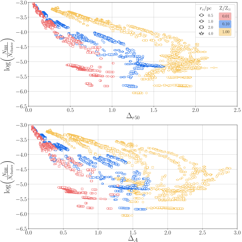
Figure 2: Number of retained BHs per cluster star ${N_{\rm{BH}}}/{N_{\rm{cluster}}}$ vs mass segregation parameters ${\Delta_{r50}}$ (top) and ${\Delta_{A}}$ (bottom), calculated between Pop2 and Pop4 under a standard radial limit of ${r_{\rm{lim}}}={r_{\rm{hl}}}$ for all model snapshots with $9\leq t\leq 13\,{\rm{Gyr}}$. Each data point represents the mean $\Delta$ across $10$ realizations of 2D projections of all stars’ radial positions in a snapshot. Uncertainty bars represent the standard deviations within these realizations. Color distinguishes models by stellar metallicity ${\rm{Z}}/{\rm{Z}}_{\odot}$, shape by virial radius $r_{v}$ (see legend). A clear anti-correlation between ${N_{\rm{BH}}}/{N_{\rm{cluster}}}$ and $\Delta$ is apparent, especially when models of particular ${\rm{Z}}$ are considered separately. In so doing, it is evident that higher ${\rm{Z}}$ results in higher $\Delta$ for any given ${N_{\rm{BH}}}/{N_{\rm{cluster}}}$. This occurs because BH masses decrease as ${\rm{Z}}$ increases. Thus, to effect the same level of quenching of $\Delta$, a higher ${N_{\rm{BH}}}/{N_{\rm{cluster}}}$ is needed. The slight backwards curvature in the trend peaking around ${N_{\rm{BH}}}/{N_{\rm{cluster}}}\sim 10^{-5}$ is due to the nondimensionalization of $\Delta$, where the half-light radius normalization factor increases faster than $\Delta$ at higher dynamical ages (generally, following the curved trajectories down from upper left). Finally, keep in mind that the number of snapshots per simulation varies significantly based on relaxation time, so this figure – unlike our calculations – does $not$ weight simulations equally.

3.3 Measuring Mass Segregation in Observed Clusters

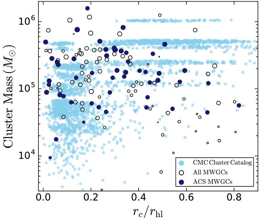
Figure 3: Total cluster mass versus $r_{c}/r_{\rm{hl}}$ for all models in the CMC Cluster Catalog (light blue; from Kremer et al., 2020), the 50 ACS Survey clusters studied in this analysis (dark blue), and the complete set of MWGCs (open circles; from Baumgardt & Hilker, 2018). The size of each dark blue and open circle corresponds to the integrated V-band magnitude of the corresponding GC (Harris, 1996, 2010 edition).

To measure $\Delta$ in real clusters, we use the ACS Survey of MWGCs (Sarajedini et al., 2007). Compiled using the wide-field channel of the Hubble Space Telescope’s Advanced Camera for Surveys (ACS), this resource catalogs stars within the central $4\arcmin\times 4\arcmin$ of 71 MWGCs and exists as an online database of stellar coordinates and calibrated photometry in the ACS VEGA-mag system (Sirianni et al., 2005). Construction of the database, which may be accessed publicly at http://www.astro.ufl.edu/~ata/public_hstgc, is fully detailed by Anderson et al. (2008).

Using the observed stellar data, we construct the same four turnoff-anchored populations as described above for the models. The exact procedure used for constructing observed populations is fully described and illustrated in Section 4 of W1. A couple important steps are worth highlighting. First, since the ACS field-of-view (FOV) is a rhombus covering only the central-most region of each GC, using raw ACS stellar data to construct the populations will introduce a radial bias in observed $\Delta$ when comparing to $\Delta$ in the models, which have effectively unlimited FOVs. We therefore establish a radial limit (${r_{\rm{lim}}}$) for each ACS-observed MWGC as the radius of the largest circle inscribable in its FOV. We then measure ${\Delta_{r50}}$ and ${\Delta_{A}}$ between each pair of the observed cluster’s three MS populations, including only stars within that specific MWGC’s radial limit. When later applying the $\Delta-{N_{\rm{BH}}},{M_{\rm{BH}}}$ correlations from the models to predict ${N_{\rm{BH}}}$ and ${M_{\rm{BH}}}$ in that MWGC, we utilize model data that has been radially-limited to match the observed ${r_{\rm{lim}}}$. For our set of 50 MWGCs, ${r_{\rm{lim}}}\in[0.52,3.48]\times{r_{\rm{hl}}}$.

Second, we found in W1 that observational incompleteness significantly impacts observed $\Delta$ measurements. Correcting for incompleteness is even more critical in this broader survey of MWGCs, as there are more extreme examples with low completeness, especially for core-collapsed clusters in which dim stars, even relatively far from the cluster center, are almost entirely washed out by the bright ones. Even in non-core-collapsed clusters, changes in $\Delta$ of order 50% are common after correcting for incompleteness.

We correct for observational incompleteness in each ACS-observed cluster using the procedure described in Section 4.3 of W1. The procedure relies on artificial star files included in the ACS Globular Cluster Survey, discussed in Section 6 of Anderson et al. (2008). In short, Anderson et al. (2008) inject $10^{5}$ artificial point spread functions (stars) into each of their raw ACS images, using the fraction of recovered to total injected stars as a proxy for true observational completeness. Using this data, we compute a kernel density estimate (KDE) of this ‘completeness fraction’ as a function of cluster-centric distance $r$ and apparent V-band magnitude $m_{V}$. Using KDEs reduces much of the uncertainty, coarseness, and bias by leveraging the full statistical power of all $10^{5}$ artificial stars compared to other methods, such as $r,m_{V}$-binning. Each observed (non-artificial) star is assigned a completeness fraction based on its location in the $(r,m_{V})$ space. While calculating $\Delta$, we randomly under-sample the stars that are more complete compared to those that are less complete by a factor given by the ratio of their completeness fractions. We repeat this exercise $10^{3}$ times to find a distribution of the measured values of $\Delta$. Thus, because of completeness differences between stars of different $r$ and $m_{V}$ in a MWGC, instead of a single value of $\Delta$, we obtain a distribution representative of the observational uncertainties for that cluster. This process and its importance are discussed in more detail in Section 4.3 of W1. We find that the uncertainties on $\Delta$ take the form of Gaussian probability density functions (PDFs) with typical $1\sigma$ uncertainty of order $10\%$ or less among the 50 ACS clusters we analyse.

In W1, we limited our analysis to 47 Tuc, M 10, and M 22 – all known to contain candidate stellar-mass BHs (e.g., Strader et al., 2012; Shishkovsky et al., 2018; Miller-Jones et al., 2015; Bahramian et al., 2017). In this full survey, we predict ${N_{\rm{BH}}}$ and ${M_{\rm{BH}}}$ for 50 of the ACS Survey’s 71 MWGCs. We do not analyze 21 GCs from the ACS catalog for varied reasons. Eight (IC04499, PAL2, PAL15, PYXIS00, RUPR106, and NGCs 0362, 6426, 7006) are excluded because the catalog does not include the necessary information (artificial star files) for performing incompleteness corrections. Three MWGCs (NGCs 6362, 6388, 6441) are excluded because their artificial star data are incomplete, two ($\omega$ Cen and NGC 6121) are excluded because their FOVs do not extend to at least 0.5 ${r_{\rm{hl}}}$, and one (NGC 6496) is excluded because its FOV is half-size and triangular rather than rhomboidal. The remaining seven of the survey’s non-NGC clusters (ARP2, E3, LYNGA7, PAL1, PAL2, TERZAN7, and TERZAN8) are excluded because of their general status as outliers relative to the bulk of the MWGCs and the limited coverage by our models of their (lower-right) region of the mass vs. $r_{c}/{r_{\rm{hl}}}$ parameter space, seen in Figure 3. In this figure, we compare the cluster properties of the selected 50 ACS Survey clusters to the full population of MWGCs (taken from Baumgardt & Hilker, 2018) as well as the models from the CMC Cluster Catalog. The figure shows that both the CMC models and the selected ACS clusters cover a very similar parameter space, providing confidence in our analysis. In addition, the analyzed clusters span roughly the entire parameter space for all MWGCs, indicating that results from this study are likely representative of the entire population of MWGCs.

3.4 Comparing Models to Observations

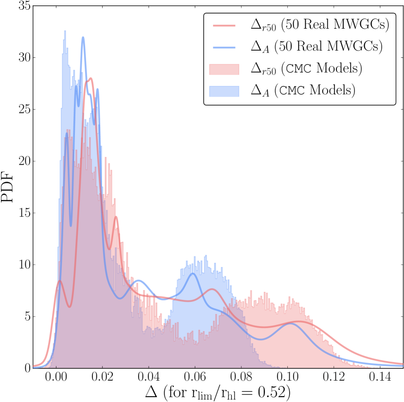
Figure 4: Normalized mass segregation distributions across all model snapshots (weighted equally; filled histograms) versus the distributions across the 50 observed MWGCs from the ACS Survey (solid curves). The ACS curves are simply normalized sums of the Gaussian PDFs representing the uncertainties on each $\Delta$ measurement after correcting for incompleteness. Here, ${\Delta_{r50}}$ (red) and ${\Delta_{A}}$ (blue) are measured between Pop2 and Pop4. To compare all modeled/observed GCs evenly, only stars within 0.52 projected half-light radii of each cluster center were included in the $\Delta$ computations, corresponding to the narrowest radial limit among the 50 ACS GCs analyzed. The close match between the CMC and ACS $\Delta$ distributions demonstrates that our models accurately capture the state of mass segregation in MWGCs, even while not having been specifically tuned to do so.

First, we compare the $\Delta$ measured in our models with those measured in the 50 MWGCs we analyze (Figure 4). Here, the $\Delta$ distribution from our models is shown as a simple normalized histogram whereas the observed distribution is obtained by summing the 50 MWGCs’ individual incompleteness-corrected $\Delta$ distributions measured in Section 3.3. In both cases we use the same radial limit (${r_{\rm{lim}}}=0.52\,{r_{\rm{hl}}}$) to ensure a fair comparison. The excellent similarity between the observed and model $\Delta$ distributions bolsters our belief that the parameter space covered in our models is representative of the MWGCs and using the $\Delta$–${N_{\rm{BH}}}$ correlation in our models to estimate ${N_{\rm{BH}}}$ for MWGCs is appropriate. For further reference, the modes and $1\sigma$ uncertainties on $\Delta$ for all MWGCs analyzed are listed in Table 1 (${\Delta_{r50}}^{24}$) and Table A1 (${\Delta_{A}}^{24}$).

The $\Delta$ distributions from our models and the MWGCs are remarkably similar, not only in range but also in rough shape. This is especially noteworthy considering how strongly the magnitude of $\Delta$ depends on the imposed radial limit and the incompleteness correction. For example, the tight limit, ${r_{\rm{lim}}}=0.52\,{r_{\rm{hl}}}$, in Figure 4 reduces the typical, unlimited value of $\Delta$ by a full order of magnitude from $\Delta\sim 0.1$ to $\Delta\sim 0.01$. Such a comparatively close match between the model and observed $\Delta$ distributions therefore provides strong evidence that our CMC models at $9$–$13\,{\rm{Gyr}}$ accurately capture the state of mass segregation in MWGCs. Furthermore, this similarity is achieved without having specifically tuned the models to match observed mass segregation; instead, the match derives simply from the observationally-motivated grid of chosen initial conditions. The match also demonstrates that our main sequence population-based method of measuring mass segregation is both highly robust and adaptable to significant FOV limitations.

Finally, it is worth pointing out that while the $\Delta$ distribution from the models appears strongly bimodal, even tetramodal, this is merely an artifact of the model grid. The four different initial virial radii divide the model set into four subsets with different initial relaxation times and accordingly divergent levels of mass segregation at late times. Variations in initial $N$ and snapshot age smooth out the resulting spectrum in $\Delta$, but the discreteness of the model grid should not be mistaken for a fundamental physical phenomenon. In turn, however, the ACS-observed $\Delta$ distribution exhibits a similarly strong peak to the model distribution at $\Delta\sim 0.02$. This specific value is unimportant, as it depends on the radial limit, but the peak’s existence does appear to be a statistically significant feature of the true mass segregation distribution for MWGCs. This peak is representative of dynamically young clusters that have yet to undergo core-collapse and retain many BHs. The tail in the distribution is also likely a true feature, representative of dynamically older clusters that have depleted most of their BHs. Together, these features likely reflect a common distribution of initial cluster size and mass in the Milky Way, contaminated by numerous dynamically-younger GCs accreted from nearby dwarf galaxies (e.g., Searle & Zinn, 1978; Mackey & Gilmore, 2004; Kruijssen et al., 2019).

4 Predicting the Number and Mass of Retained Black Holes in Observed GCs

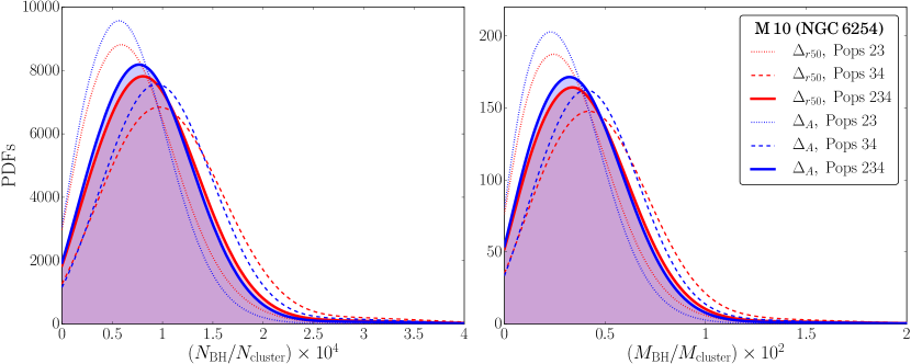
Figure 5: Example probability density functions (PDFs) for ${N_{\rm{BH}}}/{N_{\rm{cluster}}}$ and ${M_{\rm{BH}}}/{M_{\rm{cluster}}}$ in the globular cluster M 10. The complete figure set (50 images) for all MWGCs studied in this paper is available in the online journal. In all cases, the final PDFs are computed by plugging the measured, completeness-corrected mass segregation estimate ($\Delta$ as a Gaussian PDF) into a multivariate kernel density estimate (KDE) of the $\Delta$-${N_{\rm{BH}}}/{N_{\rm{cluster}}}$ ($\Delta$-${M_{\rm{BH}}}/{M_{\rm{cluster}}}$) parameter space from the models (e.g., Figure 2, except in linear scale and often with a different radial limit). Predictions made using ${\Delta_{r50}}$ are colored in red while those made using ${\Delta_{A}}$ are colored in blue. The dotted distributions correspond to predictions based only on the observed mass segregation between Pop2 and Pop3 ($\Delta^{23}$), the dashed distributions only on $\Delta^{34}$ between Pop3 and Pop4. The solid, filled distributions are based on both $\Delta^{23}$ and $\Delta^{34}$ by adding an extra dimension to the KDE (see text). The modes, $1\sigma$, and $2\sigma$ confidence intervals of these solid distributions are our final predictions, presented in Table 1. Finally, note that the x-axis tick marks are less than one, and have merely been re-scaled by the indicated factors for cleaner labeling.

We now derive PDFs for ${N_{\rm{BH}}}/{N_{\rm{cluster}}}$ and ${M_{\rm{BH}}}/{M_{\rm{cluster}}}$ retained in all 50 of the MWGCs analyzed, as inferred from the appropriate radially-limited, metallicity-matched model sets and measured ${\Delta_{r50}}$ or ${\Delta_{A}}$ (hereon referred to jointly as just $\Delta$). Unlike in W1, however, we have multiple different measurements of $\Delta$ for each cluster – one for each pairing of the three MS populations (i.e. $\Delta^{23}$, $\Delta^{24}$, $\Delta^{34}$). In order to combine the measurements into a single prediction, we compute Gaussian kernel density estimates (KDEs) of the $\Delta^{23}-\Delta^{34}-{N_{\rm{BH}}}/{N_{\rm{cluster}}}$ ($\Delta^{23}-\Delta^{34}-{M_{\rm{BH}}}/{M_{\rm{cluster}}}$) space. For those less familiar with such a method, multivariate KDEs are mere generalizations of the standard univariate KDE, a non-parametric way to estimate the PDF of a random variable. We use the standard gaussian_kde function included in SciPy’s statistics package.

For each MWGC, we select only models with ${\rm{Z}}$ closest to its observed metallicity (Harris, 1996, 2010 edition) determined on the basis of simple logarithmic binning. Specifically, BH predictions for MWGCs with ${\rm{Z}}/{\rm{Z}}_{\odot}<0.033$ are based only on the models with ${\rm{Z}}/{\rm{Z}}_{\odot}=0.01$, predictions for MWGCs with $0.033<{\rm{Z}}/{\rm{Z}}_{\odot}<0.067$ are based on models with ${\rm{Z}}/{\rm{Z}}_{\odot}=0.01$ and $0.1$, and those for MWGCs with $0.067<{\rm{Z}}/{\rm{Z}}_{\odot}<0.133$ incorporate models with ${\rm{Z}}/{\rm{Z}}_{\odot}=0.1$. For only the few MWGCs with ${\rm{Z}}/{\rm{Z}}_{\odot}>0.133$ do we use the models with ${\rm{Z}}/{\rm{Z}}_{\odot}=0.1$ and 1. In all cases, we exclude $\Delta^{24}$ as a fourth axis in the KDE because it is simply the sum of $\Delta^{23}$ and $\Delta^{34}$ and hence is not an independent additional axis. These trivariate distributions are then used to infer the expected number (total mass) of retained BHs in each GC using the following procedure.

For each GC, we evaluate the above 3D PDF (from the models) on a grid of points spanning the $3\sigma$ confidence intervals (CIs) of the observed $\Delta^{23}$ and $\Delta^{34}$, and from ${N_{\rm{BH}}}/{N_{\rm{cluster}}}$ (${M_{\rm{BH}}}/{M_{\rm{cluster}}}$) = 0 to twice the maximum ${N_{\rm{BH}}}/{N_{\rm{cluster}}}$ (${M_{\rm{BH}}}/{M_{\rm{cluster}}}$) seen in our models. The sample points are spaced evenly in linear scale along all three axes – $\Delta^{23}$, $\Delta^{34}$, and ${N_{\rm{BH}}}/{N_{\rm{cluster}}}$ (${M_{\rm{BH}}}/{M_{\rm{cluster}}}$) – with a respective grid size of $15\times 15\times 1001$ sample points. This resolution is high enough to ensure that an order of magnitude resolution increase along each axis changes the final mode, $1\sigma$ and $2\sigma$ CIs on ${N_{\rm{BH}}}/{N_{\rm{cluster}}}$ (${M_{\rm{BH}}}/{M_{\rm{cluster}}}$) in the third significant digit, at the most. In this grid form, the 3D PDF from the models is then convolved with both 1D PDFs characterizing the uncertainty on $\Delta^{23}$ and $\Delta^{34}$ observed in the MWGC (see Section 3.3). The resulting convolution is integrated numerically via Simpson’s rule (also implemented in SciPy) along the $\Delta^{23}$ and $\Delta^{34}$ axes. The integral is then normalized to obtain the final 1D PDFs for ${N_{\rm{BH}}}/{N_{\rm{cluster}}}$ (${M_{\rm{BH}}}/{M_{\rm{cluster}}}$). These distributions (filled, solid curves) are exemplified for the case of NGC 6254 (M 10) in Figure 5, based on both ${\Delta_{r50}}$ (red) and ${\Delta_{A}}$ (blue). Note that these final PDFs are equivalent to those shown in Figure 10 of W1, just with a different KDE formulation from the one used in that paper (namely, the addition of an extra axis to the KDE and convolution of the raw KDE with the observed $\Delta$ PDFs rather than Monte Carlo sampling to reduce computational cost). Versions of Figure 5 for all 50 MWGCs analyzed in this study are available in the online journal. The corresponding modes, $1\sigma$, and $2\sigma$ confidence intervals on ${N_{\rm{BH}}}/{N_{\rm{cluster}}}$ (${M_{\rm{BH}}}/{M_{\rm{cluster}}}$) for each GC are reported in Table 1 for predictions based on ${\Delta_{r50}}$. For the nearly identical results based on ${\Delta_{A}}$, see Table A1 in the Appendix. Because ${\Delta_{r50}}$ is simpler to calculate, we recommend using it in the future rather than ${\Delta_{A}}$, but we recognize that some observers seem to prefer ${\Delta_{A}}$ (e.g., Alessandrini et al., 2016).

Table 1: Cluster Properties and Raw Computational Results Based on ${\Delta_{r50}}$

Cluster	$\displaystyle{\frac{{r_{\rm{lim}}}}{{r_{\rm{hl}}}}}$	$\displaystyle{\frac{{M_{\rm{cluster}}}}{{L_{\rm{cluster}}}}}$	${M_{\rm{cluster}}}/(10^{3}\cdot{\rm{M_{\odot}}})$		${\Delta_{r50}}^{24}$	$({N_{\rm{BH}}}/{N_{\rm{cluster}}})\cdot 10^{5}$					$({M_{\rm{BH}}}/{M_{\rm{cluster}}})\cdot 10^{5}$
			Baumgardt	Harris	$\pm 1\sigma$	$-2\sigma$	$-1\sigma$	Mode	$+1\sigma$	$+2\sigma$	$-2\sigma$	$-1\sigma$	Mode	$+1\sigma$	$+2\sigma$
NGC 0104 (47Tuc)	0.55	1.77	779	1000	$0.062\pm 0.009$	0	0.41	2.75	6.87	12.1	0	13	117	302	555
NGC 0288	0.77	2.39	116	87	$0.015\pm 0.002$	1.15	6.17	11.3	16.4	22.5	39	263	512	766	1048
NGC 1261	2.45	2.12	167	225	$0.035\pm 0.014$	1.05	6.0	11.7	18.1	24.3	27	249	506	771	1043
NGC 1851	3.48	2.02	302	367	$0.104\pm 0.030$	0	0.5	3.22	7.75	14.0	0	19	139	344	624
NGC 2298	1.70	0.46	12	57	$0.032\pm 0.007$	0	1.09	4.43	8.84	14.2	0	34	177	401	690
NGC 2808	2.25	1.64	742	975	$0.058\pm 0.013$	0	1.84	5.87	10.3	15.1	0	56	212	408	631
NGC 3201	0.57	2.4	149	163	$0.013\pm 0.003$	0	2.24	13.7	27.2	62.8	0	67	602	1246	3265
NGC 4147	3.48	1.51	33	50	$0.042\pm 0.015$	0	0.65	3.55	8.44	14.3	0	28	166	411	713
NGC 4590 (M68)	1.15	2.02	123	152	$0.014\pm 0.003$	0	2.57	6.81	11.1	15.4	0	84	275	488	722
NGC 4833	0.73	0.84	247	317	$0.014\pm 0.002$	0	4.51	12.6	21.3	42.3	0	164	547	962	2090
NGC 5024 (M53)	1.29	1.59	380	521	$0.043\pm 0.010$	0	2.19	6.69	11.5	16.8	0	78	277	515	787
NGC 5053	0.68	1.66	57	87	$0.012\pm 0.001$	12.1	17.3	48.7	61.1	91.9	521	759	2443	3052	4588
NGC 5272 (M3)	0.77	1.56	394	610	$0.047\pm 0.009$	0	0.48	3.22	8.07	14.2	0	18	149	390	707
NGC 5286	2.25	1.41	401	536	$0.099\pm 0.019$	0	0.23	2.53	6.75	12.5	0	10	123	332	622
NGC 5466	0.77	1.13	46	106	$0.001\pm 0.002$	5.1	11.4	20.3	42.3	73.5	153	431	928	2001	3816
NGC 5904 (M5)	1.00	1.52	372	572	$0.040\pm 0.008$	0	1.9	6.1	11.0	16.7	0	67	243	463	724
NGC 5927	1.62	2.61	354	228	$0.015\pm 0.011$	3.43	9.74	17.4	24.4	38.5	106	373	706	1038	1726
NGC 5986	1.70	2.45	301	406	$0.021\pm 0.018$	0.35	7.21	14.1	21.2	33.0	0	285	613	955	1523
NGC 6093 (M80)	2.89	1.43	249	335	$0.120\pm 0.016$	0	0.44	3.03	7.73	13.7	0	18	143	373	672
NGC 6101	1.62	3.0	127	102	$0.002\pm 0.003$	29.4	40.9	49.1	74.7	93.0	1376	1966	2402	3918	4630
NGC 6144	1.00	0.54	45	94	$0.018\pm 0.003$	1.27	7.82	14.7	21.8	39.2	0	317	659	1008	1888
NGC 6171 (M107)	1.00	2.16	87	121	$0.018\pm 0.004$	0.03	5.23	13.2	24.8	44.2	0	207	589	1096	2078
NGC 6205 (M13)	1.00	2.61	453	450	$0.021\pm 0.006$	0	6.73	14.1	21.6	38.1	0	260	615	984	1864
NGC 6218 (M12)	0.99	1.27	87	144	$0.016\pm 0.003$	0	6.13	12.6	20.5	37.3	0	269	588	950	1742
NGC 6254 (M10)	0.89	1.94	184	168	$0.022\pm 0.003$	0	3.14	8.05	13.2	18.8	0	112	338	584	876
NGC 6304	1.29	1.37	277	142	$0.061\pm 0.025$	0	2.78	12.6	18.5	27.3	0	82	262	455	655
NGC 6341 (M92)	1.70	1.81	268	329	$0.077\pm 0.023$	0	0.65	3.47	8.28	14.0	0	26	161	402	700
NGC 6352	0.85	2.47	94	66	$0.028\pm 0.004$	0	2.78	7.53	12.5	20.6	0	104	318	549	933
NGC 6366	0.57	2.34	47	34	$0.015\pm 0.003$	0	1.88	6.58	11.8	22.2	0	61	267	514	1027
NGC 6397	0.61	2.18	89	78	$0.068\pm 0.004$	0	0	1.5	4.26	8.86	0	0	81	230	474
NGC 6535	1.99	4.8	20	14	$0.062\pm 0.015$	0	0.21	2.61	7.07	13.2	0	8	122	334	627
NGC 6541	1.62	1.42	277	438	$0.081\pm 0.020$	0	0.58	3.32	8.01	13.8	0	23	155	391	689
NGC 6584	2.45	1.12	91	204	$0.038\pm 0.018$	0	1.82	6.08	10.9	16.0	0	67	255	491	757
NGC 6624	1.99	1.02	73	169	$0.147\pm 0.051$	0	0.0	0.25	0.76	1.72	0	0	8	27	60
NGC 6637 (M69)	1.99	-	200*	195	$0.061\pm 0.026$	0	6.29	14.6	20.9	30.8	0	239	577	866	1364
NGC 6652	3.48	-	96*	79	$0.090\pm 0.032$	0	0.4	2.61	6.63	11.6	0	14	112	292	525
NGC 6656 (M22)	0.52	2.15	416	430	$0.026\pm 0.002$	0	1.13	6.61	13.3	37.8	0	39	303	624	1956
NGC 6681 (M70)	2.45	2.0	113	121	$0.080\pm 0.026$	0	1.48	5.94	11.6	19.2	0	58	256	534	898
NGC 6715 (M54)	2.25	2.04	1410	1680	$0.104\pm 0.009$	0	0.21	2.38	6.35	11.8	0	9	117	313	587
NGC 6717 (Pal9)	2.45	-	22*	31	$0.064\pm 0.020$	0	0.13	2.17	5.81	11.0	0	6	106	288	546
NGC 6723	1.15	1.77	157	232	$0.012\pm 0.005$	0.48	7.73	19.0	29.3	60.1	0	313	792	1297	2884
NGC 6752	0.91	2.17	239	211	$0.069\pm 0.013$	0	0.06	2.09	5.73	11.3	0	3	107	297	583
NGC 6779 (M56)	1.62	1.58	281	157	$0.029\pm 0.007$	0.36	4.2	9.03	13.9	18.3	0	153	380	610	829
NGC 6809 (M55)	0.61	2.38	188	182	$0.010\pm 0.002$	1.59	7.78	18.3	41.7	72.9	0	247	823	1946	3739
NGC 6838 (M71)	1.00	2.76	49	30	$0.015\pm 0.004$	0.87	6.2	17.3	31.3	61.6	0	243	740	1400	2946
NGC 6934	2.45	1.76	117	163	$0.060\pm 0.024$	0	1.3	4.98	9.62	15.1	0	47	199	414	661
NGC 6981 (M72)	1.70	-	63*	112	$0.005\pm 0.004$	4.29	13.4	21.4	34.6	48.2	152	529	908	1473	2768
NGC 7078 (M15)	1.70	1.15	453	811	$0.111\pm 0.009$	0	0.27	2.55	6.71	12.4	0	12	126	336	620
NGC 7089 (M2)	1.70	1.62	582	700	$0.109\pm 0.012$	0	0.23	2.55	6.79	12.5	0	10	124	334	624
NGC 7099 (M30)	1.70	1.85	133	163	$0.081\pm 0.017$	0	0.02	1.94	5.31	10.5	0	1	98	269	537

Note. — For each cluster (column 1), the applied radial limit from the observed data is listed in column 2. The cluster mass-to-light ratios computed in Baumgardt & Hilker (2018) are listed in column 3. Deviations form the standard mass-to-light ratio of 2 help to explain the differences between the total mass estimates in column 4-5. The mass estimates in column 4 are taken from Table 2 of Baumgardt & Hilker (2018) – except when marked by an asterisk, in which case they are not listed by the aforementioned source and are instead taken from Table 2 of Mandushev et al. (1991). Meanwhile, cluster masses in column 5 are computed from the integrated V-band magnitudes in Harris (1996, 2010 edition), assuming a uniform mass-to-light ratio of 2. Both sets of masses can be used to multiply the tabulated confidence intervals on ${N_{\rm{BH}}}/{N_{\rm{cluster}}}$ (columns 7-11) and ${M_{\rm{BH}}}/{M_{\rm{cluster}}}$ (columns 12-16) to obtain ${N_{\rm{BH}}}$ and ${M_{\rm{BH}}}$, respectively, as in Table 2. Note that the tabulated ${N_{\rm{BH}}}/{N_{\rm{cluster}}}$ and ${M_{\rm{BH}}}/{M_{\rm{cluster}}}$ predictions (columns 7-16) are based on ${\Delta_{r50}}$, specifically ${\Delta_{r50}}$ between Pop1, Pop2, and Pop3 (see text). Values based on ${\Delta_{A}}$, being nearly identical (see Figure 6), are presented in Table A1 of the Appendix. Finally, to compare mass segregation between clusters, the ${\Delta_{r50}}^{24}$ values used in Figure 4 (with the uniform choice of ${r_{\rm{lim}}}=0.52{r_{\rm{hl}}}$) are reported in column 6. These $\Delta$ values have Gaussian-shaped uncertainties imposed during the incompleteness correction. As with columns 7-16, the ${\Delta_{A}}$ version of column 6 is also reported in Table A1.

Table 2: Predicted Number and Total Mass of Retained BHs (${\Delta_{r50}}$+Baumgardt)

Cluster	${N_{\rm{BH}}}$					${M_{\rm{BH}}}\ [{\rm{M_{\odot}}}]$
	$-1\sigma$	$-2\sigma$	Mode	$+1\sigma$	$+2\sigma$	$-1\sigma$	$-2\sigma$	Mode	$+1\sigma$	$+2\sigma$
NGC 0104 (47Tuc)	0	6	43	107	189	0	101	911	2353	4323
NGC 0288	3	14	26	38	52	45	305	594	889	1216
NGC 1261	4	20	39	60	81	45	416	845	1288	1742
NGC 1851	0	3	19	47	85	0	57	420	1039	1884
NGC 2298	0	0	1	2	3	0	4	21	47	80
NGC 2808	0	27	87	153	224	0	416	1573	3027	4682
NGC 3201	0	7	41	81	187	0	100	897	1857	4865
NGC 4147	0	0	2	6	9	0	9	55	135	235
NGC 4590 (M68)	0	6	17	27	38	0	103	338	600	888
NGC 4833	0	22	62	105	209	0	405	1351	2376	5162
NGC 5024 (M53)	0	17	51	87	128	0	296	1053	1957	2991
NGC 5053	14	20	55	69	104	295	430	1383	1727	2597
NGC 5272 (M3)	0	4	25	64	112	0	71	587	1537	2786
NGC 5286	0	2	20	54	100	0	40	493	1331	2494
NGC 5466	5	10	19	39	67	70	197	423	912	1740
NGC 5904 (M5)	0	14	45	82	124	0	249	904	1722	2693
NGC 5927	24	69	123	173	273	375	1320	2499	3675	6110
NGC 5986	2	43	85	128	199	0	858	1845	2875	4584
NGC 6093 (M80)	0	2	15	38	68	0	45	356	929	1673
NGC 6101	75	104	125	190	236	1748	2497	3051	4976	5880
NGC 6144	1	7	13	20	36	0	144	299	457	855
NGC 6171 (M107)	0	9	23	43	77	0	180	512	954	1808
NGC 6205 (M13)	0	61	128	196	345	0	1178	2786	4458	8444
NGC 6218 (M12)	0	11	22	35	65	0	233	509	822	1507
NGC 6254 (M10)	0	12	30	49	69	0	206	622	1075	1612
NGC 6304	0	15	70	102	151	0	227	726	1260	1814
NGC 6341 (M92)	0	3	19	44	75	0	70	431	1077	1876
NGC 6352	0	5	14	23	39	0	98	298	515	875
NGC 6366	0	2	6	11	21	0	29	126	243	486
NGC 6397	0	0	3	8	16	0	0	72	204	421
NGC 6535	0	0	1	3	5	0	2	24	67	125
NGC 6541	0	3	18	44	76	0	64	429	1083	1909
NGC 6584	0	3	11	20	29	0	61	231	445	687
NGC 6624	0	0	0	1	3	0	0	6	20	44
NGC 6637 (M69)	0	25	58	84	123	0	478	1154	1732	2728
NGC 6652	0	1	5	13	22	0	13	107	279	501
NGC 6656 (M22)	0	9	55	111	314	0	162	1260	2596	8137
NGC 6681 (M70)	0	3	13	26	43	0	66	289	603	1015
NGC 6715 (M54)	0	6	67	179	333	0	127	1650	4413	8277
NGC 6717 (Pal9)	0	0	1	3	5	0	1	23	63	120
NGC 6723	2	24	60	92	189	0	491	1243	2036	4528
NGC 6752	0	0	10	27	54	0	7	256	710	1393
NGC 6779 (M56)	2	24	51	78	103	0	430	1068	1714	2329
NGC 6809 (M55)	6	29	69	157	274	0	464	1547	3658	7029
NGC 6838 (M71)	1	6	17	31	60	0	119	363	687	1446
NGC 6934	0	3	12	23	35	0	55	233	484	773
NGC 6981 (M72)	5	17	27	44	61	96	334	573	929	1747
NGC 7078 (M15)	0	2	23	61	112	0	54	571	1522	2809
NGC 7089 (M2)	0	3	30	79	146	0	58	722	1944	3632
NGC 7099 (M30)	0	0	5	14	28	0	1	130	358	714

Note. — Mode and mode-centric confidence intervals ($1\sigma$,$2\sigma$) are presented for ${N_{\rm{BH}}}$ and ${M_{\rm{BH}}}$ in each GC, using the Baumgardt/Mandushev masses in column 4 of Table 1 to convert from ${N_{\rm{BH}}}/{N_{\rm{cluster}}}$ and ${M_{\rm{BH}}}/{M_{\rm{cluster}}}$. These predictions are based on the mass segregation parameter ${\Delta_{r50}}$. For equivalent predictions based on ${\Delta_{A}}$, as well as the Harris masses in column 5 of Table 1, see Tables A2-A4 of the Appendix.

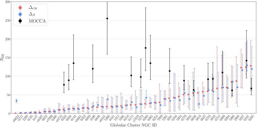
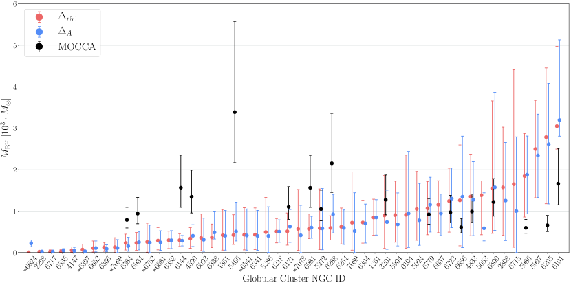
Figure 6: Number (panel 1) and total mass (panel 2) of retained BHs for each of the 50 GCs analyzed, sorted in order from lowest to highest ${N_{\rm{BH}}}$ (${M_{\rm{BH}}}$). Points and uncertainty bars represent the the mode and $1\sigma$ confidence interval, respectively. The results from both mass segregation parameters (${\Delta_{r50}}$ in red vs ${\Delta_{A}}$ in blue) are shown to give strongly consistent predictions. Simply for comparison, the predictions from the MOCCA survey (Table 2 of Askar et al., 2018) are shown in black. GCs classified as core-collapsed by Trager et al. (1995) are denoted by an asterisk.

To obtain final ${N_{\rm{BH}}}$ and ${M_{\rm{BH}}}$ estimates (not normalized by total cluster mass or star count) we assume an average stellar mass of $0.5\,{\rm{M_{\odot}}}$ and therefore multiply ${N_{\rm{BH}}}/{N_{\rm{cluster}}}$ (${M_{\rm{BH}}}/{M_{\rm{cluster}}}$) by twice (once) ${M_{\rm{cluster}}}$. We utilize the total cluster mass estimates in columns 4-5 of Table 1 based on scaled-up $N$-body simulations (Baumgardt & Hilker, 2018; Mandushev et al., 1991) as well as values computed from the integrated V-band magnitudes in Harris (1996, 2010 edition), assuming a uniform cluster mass-to-light ($M/L$) ratio of two. While the former mass values (henceforth, ‘Baumgardt/Mandushev’) are not purely observational, introducing modeling uncertainties, they do account for variation in the cluster $M/L$ ratio, which can differ significantly from the standard value of two in some GCs (see column 3 of Table 1). Meanwhile, the latter estimates (henceforth, ‘Harris’) are purely observational but do not account for variation in the $M/L$ ratio. Among the 50 GCs analyzed, the Harris mass values are only about 25% higher, on average, than those from Baumgardt/Mandushev. However, the difference exceeds a factor of two for a few clusters.

Given the above trade-off between a purely observational approach which does not consider $M/L$ variation, versus a model-based approach which does consider $M/L$ variation but possibly depends on model assumptions, we present our predicted ${N_{\rm{BH}}}$ and ${M_{\rm{BH}}}$ based on both approaches in Table 2 and Tables A2-A4, leaving it to the readers to decide which estimate is more applicable. Each table contains the modes, $1\sigma$, and $2\sigma$ CIs on ${N_{\rm{BH}}}$ and ${M_{\rm{BH}}}$ for each of the 50 GCs based on ${\Delta_{A}}$ and ${\Delta_{r50}}$, and the two mass estimates mentioned above. Since the differences between the four sets of predictions are generally small compared to the inherent uncertainties in each estimate, we focus our discussion in the rest of the paper only on the ${N_{\rm{BH}}}$ and ${M_{\rm{BH}}}$ predictions in Table 2, which is based on ${\Delta_{r50}}$ and the Baumgardt/Mandushev masses.

Figure 6 shows the modes and $1\sigma$ CIs for ${N_{\rm{BH}}}$ (top panel) and ${M_{\rm{BH}}}$ (bottom panel), using the Baumgardt/Mandushev masses. Excepting the case of NGC 6624 – the most mass-segregated cluster in our sample – the minimal effect of the choice of ${\Delta_{r50}}$ (red) versus ${\Delta_{A}}$ (blue) is evident. Furthermore, in the majority of the MWGCs analyzed ($36/50$), observed mass segregation suggests the GC retains a relatively small BH subsystem consisting of fewer than $50$ BHs with a combined mass less than $10^{3}\,{\rm{M_{\odot}}}$. Nevertheless, we can rule out zero retained BHs at $95\%$ confidence only in 13 MWGCs. Our survey pinpoints a few MWGCs that are likely to host a large BH subsystem with ${N_{\rm{BH}}}>80$ (${M_{\rm{BH}}}>1,500\,{\rm{M_{\odot}}}$): NGCs 2808, 5927, 5986, 6101, and 6205. Interestingly, Arca Sedda et al. (2018) identified the latter three as possibly hosting large BHSs. Even earlier, Peuten et al. (2016) identified NGC 6101 to contain a BHS. We identify NGCs 2808 and 5927 as two new candidates to host large BHSs.

5 The Role of Black holes in the Evolution of Core Radius

As described in Section 1, the evolution of a cluster, especially the cluster’s core structure, is tied to stellar-mass BH dynamics. When a large number of BHs are retained, the energy generated through BH burning is sufficient to delay the onset of core collapse. As the number of retained BHs decreases, so too does the cluster’s core radius ($r_{c}$), until ultimately, the core collapses completely. This connection between core structure and ${N_{\rm{BH}}}$ has been pointed out by a number of recent theoretical studies (e.g., Mackey et al., 2007, 2008; Chatterjee et al., 2017b; Kremer et al., 2018a, 2020; Askar et al., 2018).

In Figure 7, we show $r_{c}/r_{\rm{hl}}$ (taken from Harris, 1996, 2010 edition) versus our predicted ${N_{\rm{BH}}}/{N_{\rm{cluster}}}$ (left panel) and ${M_{\rm{BH}}}/{M_{\rm{cluster}}}$ (right panel) for the 50 MWGCs we have analyzed. The uncertainty bars denote $1\sigma$ confidence intervals, red and blue denote predictions using ${\Delta_{r50}}$ and ${\Delta_{A}}$, respectively. The figure shows that ${N_{\rm{BH}}}/{N_{\rm{cluster}}}$ and ${M_{\rm{BH}}}/{M_{\rm{cluster}}}$ correlate prominently with $r_{c}/{r_{\rm{hl}}}$; we predict high ${N_{\rm{BH}}}/{N_{\rm{cluster}}}$ (${M_{\rm{BH}}}/{M_{\rm{cluster}}}$) in MWGCs with large $r_{c}/{r_{\rm{hl}}}$. This validates the connection between core evolution and BH dynamics suggested in theoretical studies. For additional detail on this point, see especially Figure 3 of Kremer et al. (2020), which shows how the number (total mass) and cumulative radial distributions of BHs vary with core radius across our models. In general, nearly $100\%$ of BHs retained in our models at late times reside within the cluster’s core radius.

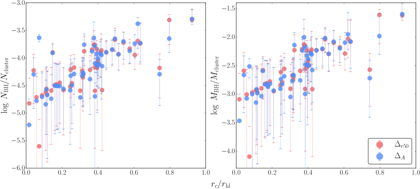
Figure 7: Number (left panel) and total mass (right panel) of retained BHs – normalized by the total number and mass of cluster stars, respectively – vs $r_{c}/{r_{\rm{hl}}}$ for each of the 50 GCs analyzed. Points and uncertainty bars represent the modes and $1\sigma$ confidence intervals, respectively. As in Figure 6, the results from both mass segregation parameters are shown (${\Delta_{r50}}$ in red, ${\Delta_{A}}$ in blue). The correlation shown here between ${N_{\rm{BH}}}/{N_{\rm{cluster}}}$ (${M_{\rm{BH}}}/{M_{\rm{cluster}}}$) and $r_{c}/{r_{\rm{hl}}}$ can be attributed to BH burning, as described in the text.

6 Comparison with Prior Results

Our primary finding is that many MWGCs contain non-negligible BH populations at present. However, the number and total mass of BHs in these populations are less than predicted in previous analyses (with some exceptions). We here discuss our predictions in relation to those prior findings, both from models and XRB observations. We especially examine the discrepancy between our results and those of Askar et al. (2018), currently the only other set of ${N_{\rm{BH}}}$ and ${M_{\rm{BH}}}$ predictions across multiple GCs.

Before comparing with results from other groups, however, it is first important to check for consistency between our new, fully developed ${N_{\rm{BH}}}$ predictions and our trial predictions presented in W1 for the MWGCs 47 Tuc, M 10 and M 22. As discussed in the preceding sections, the three primary differences between the old and new methods are the choice of populations used to quantify mass segregation, the details of the KDE formulation, and the estimated masses of observed GCs. Looking only at ${\Delta_{r50}}$ and re-scaling the old results using the new GC masses (Table 1), the new (old) ${N_{\rm{BH}}}$ predictions for these respective clusters are: $43^{+64}_{-37}$ ($21^{+57}_{-17}$), $30^{+19}_{-18}$ ($44^{+26}_{-22}$), and $55^{+56}_{-46}$ ($70^{+72}_{-48}$). The shifts (up for 47 Tuc, down for M 10 and M 22) are well within the $1\sigma$ uncertainty of the predictions. As expected, the new methodology yields results consistent with W1.

Figure 8: Comparing trends between properties of a cluster’s black hole subsystem (BHS) established by the MOCCA Survey group (Arca Sedda et al., 2018) to the same trends in our CMC models. Yellow dots (from Figure 3 of Arca Sedda et al., 2018) indicate MOCCA models at $12\,{\rm{Gyr}}$, with corresponding power law fits (gray lines; from Table A1 of Askar et al., 2018). All other dots, colored by $r_{v}$ (see legend), correspond to CMC snapshots, also with power law fits (black lines, weighting simulations equally). All parameters are defined in the text. The final panel (e) shows how weak the overall correlation is (between mass density of BHs in the BHS and the total number of BHs in GC) when these two parameters are plotted directly against one another, rather than chaining together the correlations (a-d) like Askar et al. (2018). Indeed, the direct power-law fit to the CMC models (e; black band) indicates very weak correlation (under $2\sigma$ confidence), while chaining the intermediate fits together, propagating the individual uncertainties, results in spurious correlation (e; gray band).

6.1 Comparison to MOCCA

Concurrently with the publication of W1, the creators of the MOCCA-Survey Database I – another large set of Monte Carlo cluster models similar to those produced by CMC – developed and continue to use an alternate probe of the BH content in GCs (Arca Sedda et al., 2018; Askar et al., 2018; Arca Sedda et al., 2019). Both their methodology (discussed below) and results are quite different from our mass segregation approach. We predict lower ${N_{\rm{BH}}}$ in 16 of the 18 MWGCs that the MOCCA team shortlisted as likely BHS hosts. In particularly striking examples, we rule out more than $70$ BHs (${M_{\rm{BH}}}>1800$) to 95% confidence in NGCs 0288 and 5466, both of which were predicted to have over $170$ BHs (${M_{\rm{BH}}}>2000$) in the MOCCA survey. Given these discrepancies, it is essential to more deeply examine the methodology behind the MOCCA results and the benefits or drawbacks relative to our own methods.

First, Arca Sedda et al. (2018) find a set of scaling relations between key properties of the BH subsystem that mass-segregates to the core of a GC. Specifically, they define $R_{\rm{BHS}}$ as the cluster-centric distance within which half of the total mass is in BHs (the other half of the mass is contained in stars). BHs within distance $R_{\rm{BHS}}$ from the cluster center count as members of the subsystem, which then typically contains around 60% of the total number of BHs in the models. The authors correlate $R_{\rm{BHS}}$ with number ($N_{\rm{BHS}}$) and total mass ($M_{\rm{BHS}}$) of BHs in the subsystem, and anti-correlate these three quantities with the associated BH mass density $\rho_{\rm{BHS}}=M_{\rm{BHS}}/R_{\rm{BHS}}^{3}$. Finally, they establish a tight model correlation between $\rho_{\rm{BHS}}$ and GC average surface luminosity $L/r_{\rm{hl,obs}}^{2}$, which they apply in a companion paper (Askar et al., 2018) to short-list 29 MWGCs with sizable BH subsystems, using observed V-band magnitudes and half-light radii from the Harris catalog (Harris, 1996, 2010 edition). The authors utilize a similar method to identify MWGCs that potentially host an IMBH (Arca Sedda et al., 2019).

Applying the above definitions to our own model set results in similar correlations, but a closer examination reveals several issues. The most critical concern is statistical. Whereas we use non-parametric KDEs to directly relate our observables ($\Delta^{23}$, $\Delta^{34}$) to ${N_{\rm{BH}}}/{N_{\rm{cluster}}}$ and ${M_{\rm{BH}}}/{M_{\rm{cluster}}}$, Askar et al. (2018) indirectly chain 5 separate correlations together, each with their own assumed parametric form, to relate their observable ($L_{V}/{r_{\rm{hl}}}^{2}$) to ${N_{\rm{BH}}}$. Specifically, linear curve-fits in log-log scale are applied in each of the 5 steps along the following chain: $L_{V}/{r_{\rm{hl}}}^{2}$ to $\rho_{\rm{BHS}}$ to $R_{\rm{BHS}}$ to $M_{\rm{BHS}}$ to $N_{\rm{BHS}}$ to ${N_{\rm{BH}}}$ (i.e. $N_{\rm{BH-ALL}}$, the total number of BHs in the cluster). The latter four of these power-law relations are shown in Figure 8 (a-d) for both our own model set and the MOCCA data.

Crucially, all curve fits inherently assume the parametric form used to fit the data is a true representation of the underlying statistical distribution and ignores scatter around the parametric form. They are therefore inherently biased towards the particular form used. Chaining curve fits further amplifies potential bias; the more ‘links’ in the chain, the more any deviations from a perfect fit to the underlying distribution conspire to bias the correlation.

This distorting effect is easily seen by plotting the observable directly against the dependent variable of interest. Skipping the first link in the chain ($L_{V}/{r_{\rm{hl}}}^{2}$ to $\rho_{\rm{BHS}}$), we plot $\rho_{\rm{BHS}}$ vs ${N_{\rm{BH}}}$ in the bottom panel of Figure 8, bypassing the intermediate variables $R_{\rm{BHS}}$, $M_{\rm{BHS}}$, and $N_{\rm{BHS}}$. Applying a single, unchained least-squares fit to the CMC data (black band), it is evident that there is only a very weak anti-correlation between $\rho_{\rm{BHS}}$ and ${N_{\rm{BH}}}$. This contradicts the analysis by Askar et al. (2018); chaining together their step-wise correlations from the upper panels results in a much larger anti-correlation between $\rho_{\rm{BHS}}$ and ${N_{\rm{BH}}}$ (gray band). Propagating uncertainty, the $1\sigma$ confidence interval (gray band) on predicted ${N_{\rm{BH}}}$ spans nearly 2 orders of magnitude for any given value of $\rho_{\rm{BHS}}$. The inflated uncertainty partially mitigates, but does not eliminate, the underlying bias introduced from chaining multiple parametric fits.

As mentioned in Section 2.6 of Askar et al. (2018), models without ${N_{\rm{BH}}}>15$ at $12\,{\rm{Gyr}}$ were excluded from their analysis. Of these excluded models, most incorporated high BH natal kicks, but $\sim 40$ utilized the standard mass fallback prescription (Belczynski et al., 2002) and had similar values of the observable ($L_{V}/{r_{\rm{hl}}}^{2}$) to the $163$ included models, despite having significantly fewer BHs (${N_{\rm{BH}}}<15$). This indicates that $L_{V}/{r_{\rm{hl}}}^{2}$ may not actually be a strong predictor of the BH content in GCs, supporting our findings in the bottom panel of Figure 6. At the very least, excluding the 20% of models with lowest ${N_{\rm{BH}}}$ would naturally cause the MOCCA team to over-predict ${N_{\rm{BH}}}$ and ${M_{\rm{BH}}}$, partially explaining why our analysis generally yields lower predictions.

6.2 Possible Sources of Uncertainties in Our Predictions

Although our analysis based on the CMC catalog benefits from non-parametric statistical methods that are generally less prone to bias than parametric methods – especially the MOCCA team’s chaining technique – the models from the MOCCA database do present their own advantages. Whereas the models in the CMC Catalog all start with a primordial binary fraction $f_{b}=5\%$, expected to be typical of the MWGCs, the MOCCA models initialize with a variety of binary fractions, ranging from $f_{b}=5\%$ all the way up to $95\%$ (Askar et al., 2017b). Though we found in W1 that shifting $f_{b}$ between $5\%$ and $10\%$ had no distinguishable impact on the anti-correlation between $\Delta$ and ${N_{\rm{BH}}}$, it is conceivable that higher binary fractions could impact the correlation. This possibility could favor the MOCCA team’s ${N_{\rm{BH}}}$ (${M_{\rm{BH}}}$) predictions for any GC where the true $f_{b}$ is much greater than $5\%$.

Other potential improvements to both our own analysis and that of the MOCCA team may include consideration of primordial mass segregation and non-standard initial mass functions. Although the former is expected to have little effect after several relaxation times, it may accelerate the dynamical evolution of BHs. In addition, primordial mass segregation may change the BH mass function via collisions and accretions onto the BHs (Kremer et al., 2020), thus indirectly affecting mass segregation.

Meanwhile, the choice of IMF, especially the slope for the high-mass stars, has a dramatic impact on cluster evolution in general (e.g., Chatterjee et al., 2017b). However, the effects of non-standard IMFs on the $\Delta$–${N_{\rm{BH}}}$ (${M_{\rm{BH}}}$) anti-correlation may be more subtle. Any IMF that simply changes the total number and average mass of the BHs themselves may not significantly affect the predicted numbers – fewer or less-massive BHs would still lead to higher $\Delta$. This robustness is in fact a unique feature of our approach. Perhaps more likely to affect the anti-correlation are IMFs which fundamentally alter the relative importance of other dynamically influential populations, such as neutron stars. Additionally, if we assume that the non-standard IMF varies from cluster-to-cluster, then the inherent spread in the $\Delta$–${N_{\rm{BH}}}/{N_{\rm{cluster}}}$ anti-correlation in our models will likely increase (Figure 2), swelling the uncertainty on ${N_{\rm{BH}}}$ (${M_{\rm{BH}}}$) predicted in real MWGCs. Further studying the late-time effects of both primordial mass segregation and non-standard IMFs may therefore prove illuminating in future work.

Ultimately, we find that quantities like $\Delta$ that parameterize mass segregation are a more reliable statistical predictor of the total mass and number of BHs inside a GC than the $L_{V}/{r_{\rm{hl}}}^{2}$-BHS correlations used in the MOCCA survey (Arca Sedda et al., 2018; Askar et al., 2018; Arca Sedda et al., 2019), This, at least, is true independently of any other advantages or disadvantages (discussed above) associated with the specific model sets the analysis must rely upon.

Constituting the largest sample of GCs for which BH populations have been reported to-date, our analysis suggests while some BH retention is common to many GCs, fewer are retained – generally less than $50$ – than has typically been suggested previously. In addition to this general point, we discuss findings of particular interest for specific MWGCs in the following subsections.

6.3 47 Tuc

As one of the nearest and therefore most well-studied GCs, 47 Tuc (NGC 0104) is an important cluster for benchmarking. The cluster’s mass of around $10^{6}\,{\rm{M_{\odot}}}$ (Table 1) is near the maximum of our model space at $13\,{\rm{Gyr}}$, but its Galactocentric distance and metallicity are well within the model bounds (Harris, 1996, 2010 edition). In W1, our ${N_{\rm{BH}}}$ predictions for 47 Tuc were limited by a dearth of models with high mass segregation. Now, without such a limitation, we predict the cluster retains more BHs, around 40 totalling 900 ${\rm{M_{\odot}}}$. This new estimate is still well within $1\sigma$ of the estimate in W1. Our current estimate is also consistent to $1\sigma$ with a contemporary study to specifically model 47 Tuc that predicts a relatively small BHS in the cluster (Hénault-Brunet et al., 2020). Note however, at 95% confidence, we can neither exclude zero BHs nor a large population of up to $\sim 200$ BHs totalling 4,300 ${\rm{M_{\odot}}}$ in 47 Tuc.

6.4 NGC 2808

Lützgendorf et al. (2012a) previously found five high-velocity giants in the core of NGC 2808 and suggested their extreme velocities could have resulted from close encounters with a stellar-mass BH or IMBH, but most likely the former with a mass of about 10 ${\rm{M_{\odot}}}$. In follow-up analysis with Monte Carlo 3-body scattering experiments, they further solidified this hypothesis and constrained the maximum mass of the BH to be no more than $10^{4}\,{\rm{M_{\odot}}}$ (Lützgendorf et al., 2012b). These prior findings fit well with our observation that NGC 2808 is one of the least mass-segregated clusters in the MW. The low observed $\Delta$ leads to our prediction that NGC 2808 contains around 90 BHs totalling 1,500 ${\rm{M_{\odot}}}$ in mass (Table 2). Taken together, these lines of evidence strongly suggest that NGC 2808 presently retains a robust central BH population.

6.5 NGC 3201

Recently, Giesers et al. (2018) reported a stellar-mass BH in the cluster NGC 3201. They inferred the BH’s presence from the large radial velocity variations ($\sim 100$ km/s) of an apparently lone main sequence star, thereby presumed to be orbiting a compact remnant. This detection – along with two more recent ones (Giesers et al., 2019) – made NGC 3201 the fifth MWGC known to harbor a stellar-mass BH candidate. Shortly thereafter, Kremer et al. (2018b) used CMC to model the cluster, reporting that it likely retains $>200$ stellar-mass BHs at present, an estimate that was revised down to ${N_{\rm{BH}}}=120\pm 10$ in a follow-up using updated BH formation physics (Kremer et al., 2019). This revised prediction is in line with the MOCCA team’s estimate, ${N_{\rm{BH}}}=114^{+60}_{-35}$ (Askar et al., 2018), but mass segregation predicts an even lower number: ${N_{\rm{BH}}}=41^{+40}_{-34}$.

6.6 NGC 6101

Of the 50 MWGCs surveyed, NGC 6101 is the least mass-segregated and is by far the best candidate in which to find a large number of BHs. To 95% confidence, we estimate it contains $75-236$ BHs with a combined mass of $1,750-5,900\,{\rm{M_{\odot}}}$. Most likely, it contains $\sim 125$ BHs totalling $\sim 3,000\,{\rm{M_{\odot}}}$. This conclusion is supported by a growing body of evidence from other sources. Dalessandro et al. (2015) were the first to draw attention to this GC’s unusually low mass segregation, finding no evidence for the phenomenon based on three different measures: the radial distribution of blue stragglers, that of MS binaries, and the luminosity function. Following this finding, Peuten et al. (2016) and Webb et al. (2017) explored the anti-correlation between ${N_{\rm{BH}}}$ and mass segregation in $N$-body simulations to demonstrate that the cluster may contain a large population of BHs. Baumgardt & Sollima (2017) disputed these suggestions because their estimates of NGC 6101’s mass-function slope indicated mass segregation after all. However, given that this rebuttal relies on the same ACS dataset as applied in this study and because their results similarly suggest that NGC 6101 has one of the lowest levels of mass segregation among MWGCs, we find no contradiction to our conclusions; NGC 6101 is very likely to host a robust population of stellar-mass BHs. This determination is further supported by the findings of Askar et al. (2018) discussed above.

6.7 NGC 6535

NGC 6535 is unusual in that it’s relatively old but has a high mass-to-light ratio in the range 5 (Baumgardt & Hilker, 2018) to 11 (Zaritsky et al., 2014). Halford & Zaritsky (2015) found that its observed mass-function has a positive slope – indicating a high loss-rate of low-mass stars and making its high $M/L$ ratio even more puzzling. Given NGC 6535’s small Galactocentric distance of $3.9$ kpc (Harris, 1996, 2010 edition), it is likely that increased tidal stripping of low-mass stars near the Galactic center is responsible for the positive mass-function slope. However, Halford & Zaritsky (2015) found no evidence that clusters near the Galactic center with similarly top-heavy mass functions had artificially inflated mass estimates, raising the possibility that some dark mass may be responsible for NGC 6535’s high $M/L$ ratio. Recently, Askar et al. (2017a) demonstrated that $N$-body simulations of clusters containing an IMBH or BHS were able to fit the photometric and kinematic properties of NGC 6535, but later concluded the cluster contains neither a significant BHS nor an IMBH (Askar et al., 2018; Arca Sedda et al., 2019). Since we rule out more than $130\,{\rm{M_{\odot}}}$ of BHs in NGC 6535 to 95% confidence, the mystery of the apparently missing mass in this cluster remains an open question.

6.8 NGC 6624

Perera et al. (2017) reported the possible presence of an IMBH in NGC 6624 based on timing observations of a millisecond pulsar near the projected cluster center. Their timing analysis indicated the presence of an IMBH with mass in the range 7,500 to 10,000 ${\rm{M_{\odot}}}$, even up to 60,000 ${\rm{M_{\odot}}}$. This finding was disputed by Gieles et al. (2018), who demonstrated that dynamical models without an IMBH produce maximum accelerations at the pulsar’s position comparable to its observed line-of-sight acceleration. Recently, Baumgardt et al. (2019) similarly found that their $N$-body models without an IMBH could provide excellent fits to the observed velocity dispersion and surface brightness profiles (VDPs and SDPs) in NGC 6624. Their cluster models with an IMBH indicated that an IMBH in NGC 6624 with mass $>$1,000 ${\rm{M_{\odot}}}$ was incompatible with the cluster’s observed VDP and SBP. Meanwhile, based on data from HST and ATCA, Tremou et al. (2018) found that all radio emissions observed from NGC 6624 are consistent with being from a known ultra-compact X-ray binary in the cluster’s core. Their radio observations place a $3\sigma$ upper limit on the cluster’s possible IMBH mass of 1,550 ${\rm{M_{\odot}}}$. Although we have yet to explore how much difference an IMBH has on quenching $\Delta$ compared to a BHS, our results support the latter three studies; we find to 95% confidence that there are no more than $\sim 400\,{\rm{M_{\odot}}}$ of BHs in NGC 6624 (using Baumgardt’s cluster mass, otherwise $<\sim 900\,{\rm{M_{\odot}}}$ of BHs using Harris’ cluster mass). Indeed, NGC 6624 is the most mass-segregated cluster in our sample, suggesting that it may in fact be one of the MWGCs least likely to host an IMBH or significant BHS.

6.9 M 54

Thought to be a MWGC for over two centuries, the cluster M 54 (NGC 6715) is now known to be coincident with the center of the Sagittarius Dwarf Galaxy (e.g., Monaco et al., 2005), perhaps even as the galaxy’s original nucleus (Layden & Sarajedini, 2000). While M 54’s metallicity is well-covered by our model parameter space, its effective Galactocentric distance is unreliable because our models assume a MW-like potential for tidal boundary calculations. Its approximate mass is also at the extreme upper end of the model space (Table 1). Therefore, with some reservation, despite M 54’s highly mass-segregated present state, we predict a significant number of BHs remain in the cluster at present, with $67^{+112}_{-61}$ BHs totalling around $1,650^{+2,763}_{-1,523}$ ${\rm{M_{\odot}}}$. This prediction is consistent with the $3\sigma$ upper limit on a single accreting IMBH of $<3,000\,{\rm{M_{\odot}}}$ imposed by VLA radio observations (Tremou et al., 2018).

6.10 NGC 6723

NGC 6723 is listed as possibly core-collapsed in the Harris catalog (Harris, 1996, 2010 edition), an identification which would appear at odds with our relatively high prediction for ${N_{\rm{BH}}}$ and ${M_{\rm{BH}}}$ in this GC (Figure 6, Table 2). However, Table 2 of Trager et al. (1995), the purported source material for the Harris catalog’s core-collapsed classifications, lists NGC 6723 as non-core-collapsed. Their surface brightness profile for the cluster also shows a flat core density, further contradicting the Harris classification. We speculate that the Harris catalog may have accidentally swapped the core-collapse classifications between NGCs 6723 and 6717 (Palomar 9), which appear consecutively in Table 2 of (Trager et al., 1995). For this reason, we do not mark this MWGC as core-collapsed in Figure 6.

7 Summary & Discussion

7.1 Summary

We have presented a statistically robust method that uses mass segregation between easily observable stellar populations to determine the number of BHs in a cluster. Our process can be implemented for any observed MWGC and carefully accounts for potential sources of bias between models and observations, including field-of-view limits, projection effects, and observational incompleteness. Due to the expansive grid of realistic cluster models used, the process also accounts for many uncertainties on cluster initial conditions. We briefly summarize our key findings below.

1. We demonstrated that, overall, the CMC Cluster Catalog models yield mass segregation ($\Delta$) values which closely match the observed distribution in $\Delta$ among real MWGCs (see Figure 4). This provides strong evidence that our models capture the state of mass segregation in realistic MWGCs, complementing the results of Kremer et al. (2020).

2. By using $\Delta$ as a predictive parameter, we have constrained the total number and mass in stellar-mass BHs contained in more MWGCs, 50 total, than any prior studies.

3. We find that 35 of the 50 GCs studied retain more than 20 BHs at present and 8 retain more than 80 BHs. These predictions indicate that present-day BH retention is common to many MWGCs, though to a lesser extent than suggested in competing analyses, (e.g., Askar et al., 2018).

4. Specifically, we have identified NGCs 2808, 5927, 5986, 6101, and 6205 to contain especially large BH populations, each with total BH mass exceeding $10^{3}\,{\rm{M_{\odot}}}$. These clusters may serve as ideal observational targets for BH candidate searches.

5. We also explored in detail the advantages and disadvantages of our statistical methods compared to other similar analyses in the literature.

7.2 Discussion and Future Work

Here, we predict smaller BH populations in a few GCs compared to our previous analyses which also utilized CMC models (e.g., Kremer et al., 2019). The exact number of BHs is highly uncertain (indeed, this is reflected by the uncertainty bars in Figure 6 and all the tables). Hence, discrepancy between these results and those of our previous work – which implemented entirely different methods based on fitting surface brightness and velocity dispersion profiles to predict ${N_{\rm{BH}}}$ – is unsurprising. Critically, as shown in Figure 7, the overall connection between cluster core evolution and BH dynamics put forward in previous work (Mackey et al., 2008; Kremer et al., 2018b, 2019) is confirmed. This further validates the significant role BHs play in GC evolution.

There are a couple of more speculative conclusions hinted at by our results which are worth mentioning briefly, but require additional study. First, it is tempting to extrapolate our predictions of total BH mass in GCs to place upper limits on the masses of possible intermediate-mass black holes (IMBHs) in those clusters. Indeed, $N$-body simulations have shown that an IMBH of mass $>1\%$ of its host GC’s overall mass should significantly quench mass segregation – even among only visible giants and MS stars (e.g., Gill et al., 2008; Pasquato et al., 2016). The generally significant mass segregation we measure in the 50 GCs studied – representative of the MW as a whole – therefore suggests that IMBHs with mass $>$1,000 ${\rm{M_{\odot}}}$ are rare in MWGCs. However, firmer constraints would require testing beyond the scope of this study, specifically on how similar the dynamical impact of a single IMBH is to that of a stellar-mass BH population with identical total mass. Is it a one-to-one relation, or does a, for example, $1,000\,{\rm{M_{\odot}}}$ IMBH perhaps have a much weaker effect on mass segregation than a population of a hundred $10\,{\rm{M_{\odot}}}$ BHs? For now, the prospect of IMBHs in GCs is still best analyzed through direct observations in the X-ray and radio bands, as well as via the accelerations of luminous stars within the IMBH’s ‘influence radius,’ but further study may be able to extend our constraints on stellar-mass BH populations to IMBHs in GCs.

Second, it has been suggested that clusters were born already mass-segregated to a degree, a property termed ‘primordial’ mass segregation (e.g., Baumgardt et al., 2008). Our models assume clusters have no primordial mass segregation. Hence, the close match between $\Delta$ in our models and the $\Delta$ distribution observed in the MWGCs (see Figure 4) demonstrates that our models do not need to start off with some degree of mass segregation to match real clusters. This finding could suggest that primordial mass segregation is minimal or non-existent in the MWGCs, but such a conclusion is tenuous since primordial mass segregation is likely to be washed out at the present day after many relaxation times. Further consideration of the late-time effects of primordial mass segregation on presently observable $\Delta$ is necessary to make any further conclusions on this matter.

Finally, although mass segregation has been shown here to be a strong indicator of BH populations in clusters, recent analyses have shown that many other observables, including millisecond pulsars (Ye et al., 2019), blue stragglers (Kremer et al., 2020), and cluster surface brightness and velocity dispersion profiles (e.g., Mackey et al., 2008; Kremer et al., 2018b), may also correlate with BH dynamics and thus may also serve as indicators of retained BH numbers. In order to pin down more precisely the true number of BHs retained in specific clusters, all of these observables should be leveraged in tandem. We intend to pursue such analysis further in future works.

Table A1: Cluster Properties and Raw Computational Results Based on ${\Delta_{A}}$

Cluster	$\displaystyle{\frac{{r_{\rm{lim}}}}{{r_{\rm{hl}}}}}$	$\displaystyle{\frac{{M_{\rm{cluster}}}}{{L_{\rm{cluster}}}}}$	${M_{\rm{cluster}}}/(10^{3}\cdot{\rm{M_{\odot}}})$		${\Delta_{A}}^{24}$	$({N_{\rm{BH}}}/{N_{\rm{cluster}}})\cdot 10^{5}$					$({M_{\rm{BH}}}/{M_{\rm{cluster}}})\cdot 10^{5}$
			Baumgardt	Harris	$\pm 1\sigma$	$-2\sigma$	$-1\sigma$	Mode	$+1\sigma$	$+2\sigma$	$-2\sigma$	$-1\sigma$	Mode	$+1\sigma$	$+2\sigma$
NGC 0104 (47Tuc)	0.55	1.77	779	1000	$0.052\pm 0.006$	0	0.41	2.67	6.8	11.9	0	16	121	313	558
NGC 0288	0.77	2.39	116	87	$0.008\pm 0.001$	2.24	9.93	18.2	26.6	46.9	44	408	797	1202	2219
NGC 1261	2.45	2.12	167	225	$0.020\pm 0.010$	1.25	6.02	11.6	18.1	23.6	40	253	507	764	1004
NGC 1851	3.48	2.02	302	367	$0.093\pm 0.032$	0	0.52	3.11	7.61	13.2	0	19	134	336	590
NGC 2298	1.70	0.46	12	57	$0.022\pm 0.003$	0	1.63	5.41	9.68	14.5	0	53	215	432	696
NGC 2808	2.25	1.64	742	975	$0.067\pm 0.009$	0	1.3	4.74	8.87	13.4	0	39	169	358	578
NGC 3201	0.57	2.4	149	163	$0.012\pm 0.001$	0	1.8	11.3	22.1	54.9	0	53	494	1010	2810
NGC 4147	3.48	1.51	33	50	$0.043\pm 0.009$	0	0.44	3.09	7.88	14.0	0	20	151	391	698
NGC 4590 (M68)	1.15	2.02	123	152	$0.014\pm 0.002$	0.12	3.49	7.97	12.5	16.8	0	119	329	547	772
NGC 4833	0.73	0.84	247	317	$0.011\pm 0.001$	0	4.47	11.9	19.7	38.5	0	165	515	888	1864
NGC 5024 (M53)	1.29	1.59	380	521	$0.034\pm 0.006$	0	1.4	5.12	9.72	15.0	0	46	205	439	714
NGC 5053	0.68	1.66	57	87	$0.005\pm 0.001$	7.3	12.6	22.4	52.0	83.6	291	497	1037	2546	4276
NGC 5272 (M3)	0.77	1.56	394	610	$0.036\pm 0.006$	0	0.42	3.12	8.01	14.3	0	17	148	392	716
NGC 5286	2.25	1.41	401	536	$0.099\pm 0.012$	0	0.02	2.01	5.5	10.9	0	1	100	275	548
NGC 5466	0.77	1.13	46	106	$0.004\pm 0.001$	9.64	15.0	41.7	54.1	83.2	400	610	1115	2664	4261
NGC 5904 (M5)	1.00	1.52	372	572	$0.033\pm 0.005$	0	1.27	4.77	9.28	14.5	0	43	183	387	626
NGC 5927	1.62	2.61	354	228	$0.016\pm 0.006$	2.62	9.62	16.4	22.4	32.9	78	375	662	943	1447
NGC 5986	1.70	2.45	301	406	$0.019\pm 0.011$	0.96	7.67	14.2	20.9	29.6	4	310	624	934	1314
NGC 6093 (M80)	2.89	1.43	249	335	$0.111\pm 0.012$	0	0.27	2.59	6.82	12.5	0	11	124	333	618
NGC 6101	1.62	3.0	127	102	$0.003\pm 0.002$	35.8	44.6	50.9	76.6	94.7	1665	2211	2518	4043	4693
NGC 6144	1.00	0.54	45	94	$0.011\pm 0.002$	1.28	8.01	13.4	18.9	25.9	30	357	632	909	1253
NGC 6171 (M107)	1.00	2.16	87	121	$0.015\pm 0.002$	1.18	7.22	17.4	27.2	45.7	13	283	721	1195	2106
NGC 6205 (M13)	1.00	2.61	453	450	$0.013\pm 0.004$	0	6.59	13.2	19.9	32.7	0	259	577	901	1553
NGC 6218 (M12)	0.99	1.27	87	144	$0.011\pm 0.002$	0	6.58	12.7	20.0	35.6	0	286	583	912	1523
NGC 6254 (M10)	0.89	1.94	184	168	$0.018\pm 0.002$	0	3.01	7.67	12.6	17.7	0	107	324	559	827
NGC 6304	1.29	1.37	277	142	$0.050\pm 0.015$	0	3.23	12.3	17.3	24.1	0	83	254	422	591
NGC 6341 (M92)	1.70	1.81	268	329	$0.066\pm 0.015$	0	0.52	3.18	7.84	13.7	0	20	149	379	681
NGC 6352	0.85	2.47	94	66	$0.017\pm 0.002$	0	2.91	7.88	13.7	21.1	0	102	317	563	924
NGC 6366	0.57	2.34	47	34	$0.015\pm 0.001$	0	1.37	5.07	9.38	16.7	0	39	190	393	785
NGC 6397	0.61	2.18	89	78	$0.059\pm 0.003$	0	0	0.61	1.8	4.06	0	0	34	100	226
NGC 6535	1.99	4.8	20	14	$0.037\pm 0.006$	0	2.45	7.11	11.3	15.4	0	72	264	478	713
NGC 6541	1.62	1.42	277	438	$0.068\pm 0.013$	0	0.5	3.11	7.71	13.5	0	21	149	380	677
NGC 6584	2.45	1.12	91	204	$0.025\pm 0.011$	0	0.94	4.12	8.8	14.2	0	33	174	407	690
NGC 6624	1.99	1.02	73	169	$0.125\pm 0.038$	0.7	19.6	23.2	26.8	31.1	73	193	305	416	525
NGC 6637 (M69)	1.99	-	200*	195	$0.046\pm 0.017$	0.3	5.39	11.8	17.3	22.7	0	205	472	705	951
NGC 6652	3.48	-	96*	79	$0.077\pm 0.023$	0	0.51	2.75	6.68	11.3	0	17	115	292	511
NGC 6656 (M22)	0.52	2.15	416	430	$0.018\pm 0.001$	0	1.02	7.11	14.5	40.9	0	29	324	675	2104
NGC 6681 (M70)	2.45	2.0	113	121	$0.075\pm 0.016$	0	1.21	5.02	10.1	16.3	0	47	216	466	770
NGC 6715 (M54)	2.25	2.04	1410	1680	$0.074\pm 0.007$	0	0	1.44	3.95	8.36	0	0	71	198	420
NGC 6717 (Pal9)	2.45	-	22*	31	$0.047\pm 0.011$	0	0.15	2.13	5.67	10.7	0	6	104	277	528
NGC 6723	1.15	1.77	157	232	$0.010\pm 0.003$	1.69	9.44	19.9	29.4	59.5	34	382	828	1299	2853
NGC 6752	0.91	2.17	239	211	$0.054\pm 0.007$	0	0.02	1.96	5.35	10.6	0	1	100	277	548
NGC 6779 (M56)	1.62	1.58	281	157	$0.019\pm 0.004$	0.65	4.81	9.8	14.7	19.4	5	176	411	646	865
NGC 6809 (M55)	0.61	2.38	188	182	$0.009\pm 0.001$	1.9	8.51	18.6	43.5	73.8	16	284	837	2057	3786
NGC 6838 (M71)	1.00	2.76	49	30	$0.008\pm 0.002$	9.36	16.4	23.0	44.7	69.7	365	664	990	2038	3315
NGC 6934	2.45	1.76	117	163	$0.052\pm 0.016$	0	1.38	5.18	10.1	15.7	0	54	214	433	681
NGC 6981 (M72)	1.70	-	63*	112	$0.003\pm 0.003$	6.02	13.1	22.3	31.4	45.5	235	547	957	1388	2103
NGC 7078 (M15)	1.70	1.15	453	811	$0.102\pm 0.006$	0	0	1.82	4.98	10.0	0	0	92	252	507
NGC 7089 (M2)	1.70	1.62	582	700	$0.101\pm 0.008$	0	0	1.92	5.29	10.6	0	0	89	248	502
NGC 7099 (M30)	1.70	1.85	133	163	$0.067\pm 0.011$	0	0	1.67	4.6	9.39	0	0	84	235	481

Note. — This table is identical to Table 1, except based on ${\Delta_{r50}}$ instead of ${\Delta_{A}}$. Specifically, column 6 lists the ${\Delta_{A}}^{24}$ values used in Figure 4 (with the uniform choice of ${r_{\rm{lim}}}=0.52{r_{\rm{hl}}}$). Again, these $\Delta$ values have Gaussian-shaped uncertainties imposed during the incompleteness correction. Similarly, the ${N_{\rm{BH}}}/{N_{\rm{cluster}}}$ and ${M_{\rm{BH}}}/{M_{\rm{cluster}}}$ predictions listed in columns 7-16 are based on ${\Delta_{A}}$ between Pop1, Pop2, and Pop3 (see Section 4).

Table A2: Predicted Number and Mass of Retained BHs (${\Delta_{A}}$+Baumgardt)

Cluster	${N_{\rm{BH}}}$					${M_{\rm{BH}}}\ [{\rm{M_{\odot}}}]$
	$-1\sigma$	$-2\sigma$	Mode	$+1\sigma$	$+2\sigma$	$-1\sigma$	$-2\sigma$	Mode	$+1\sigma$	$+2\sigma$
NGC 0104 (47Tuc)	0	6	42	106	185	0	125	943	2438	4347
NGC 0288	5	23	42	62	109	51	473	925	1394	2574
NGC 1261	4	20	39	60	79	67	423	847	1276	1677
NGC 1851	0	3	19	46	80	0	57	405	1015	1782
NGC 2298	0	0	1	2	3	0	6	25	50	81
NGC 2808	0	19	70	132	199	0	289	1254	2656	4289
NGC 3201	0	5	34	66	164	0	79	736	1505	4187
NGC 4147	0	0	2	5	9	0	7	50	129	230
NGC 4590 (M68)	0	9	20	31	41	0	146	405	673	950
NGC 4833	0	22	59	97	190	0	408	1272	2193	4604
NGC 5024 (M53)	0	11	39	74	114	0	175	779	1668	2713
NGC 5053	8	14	25	59	95	165	281	587	1441	2420
NGC 5272 (M3)	0	3	25	63	113	0	67	583	1544	2821
NGC 5286	0	0	16	44	87	0	4	401	1103	2197
NGC 5466	9	14	38	49	76	182	278	508	1215	1943
NGC 5904 (M5)	0	9	35	69	108	0	160	681	1440	2329
NGC 5927	19	68	116	159	233	276	1328	2343	3338	5122
NGC 5986	6	46	85	126	178	12	933	1878	2811	3955
NGC 6093 (M80)	0	1	13	34	62	0	27	309	829	1539
NGC 6101	91	113	129	195	241	2115	2808	3198	5135	5960
NGC 6144	1	7	12	17	23	14	162	286	412	568
NGC 6171 (M107)	2	13	30	47	80	11	246	627	1040	1832
NGC 6205 (M13)	0	60	120	180	296	0	1173	2614	4082	7035
NGC 6218 (M12)	0	11	22	35	62	0	247	504	789	1317
NGC 6254 (M10)	0	11	28	46	65	0	197	596	1029	1522
NGC 6304	0	18	68	96	134	0	230	704	1169	1637
NGC 6341 (M92)	0	3	17	42	73	0	54	399	1016	1825
NGC 6352	0	5	15	26	40	0	96	297	528	867
NGC 6366	0	1	5	9	16	0	18	90	186	371
NGC 6397	0	0	1	3	7	0	0	30	89	201
NGC 6535	0	1	3	5	6	0	14	53	96	143
NGC 6541	0	3	17	43	75	0	58	413	1053	1875
NGC 6584	0	2	7	16	26	0	30	158	369	626
NGC 6624	1	29	34	39	45	53	141	223	304	384
NGC 6637 (M69)	1	22	47	69	91	0	410	944	1410	1902
NGC 6652	0	1	5	13	22	0	16	110	279	488
NGC 6656 (M22)	0	8	59	121	340	0	121	1348	2808	8753
NGC 6681 (M70)	0	3	11	23	37	0	53	244	527	870
NGC 6715 (M54)	0	0	41	111	236	0	0	1001	2792	5922
NGC 6717 (Pal9)	0	0	1	2	5	0	1	23	61	116
NGC 6723	5	30	62	92	187	53	600	1300	2039	4479
NGC 6752	0	0	9	26	51	0	2	239	662	1310
NGC 6779 (M56)	4	27	55	83	109	14	495	1155	1815	2431
NGC 6809 (M55)	7	32	70	164	277	30	534	1574	3867	7118
NGC 6838 (M71)	9	16	23	44	68	179	326	486	1001	1628
NGC 6934	0	3	12	24	37	0	63	250	507	797
NGC 6981 (M72)	8	17	28	40	57	148	345	604	876	1327
NGC 7078 (M15)	0	0	16	45	91	0	0	417	1142	2297
NGC 7089 (M2)	0	0	22	62	123	0	0	518	1443	2922
NGC 7099 (M30)	0	0	4	12	25	0	0	112	313	640

Note. — Mode and mode-centric confidence intervals ($1\sigma$,$2\sigma$) are presented for ${N_{\rm{BH}}}$ and ${M_{\rm{BH}}}$ in each GC, using the Baumgardt/Mandushev masses in column 4 of Table 1 to convert from ${N_{\rm{BH}}}/{N_{\rm{cluster}}}$ and ${M_{\rm{BH}}}/{M_{\rm{cluster}}}$. These predictions are based on the mass segregation parameter ${\Delta_{A}}$.

Table A3: Predicted Number and Mass of Retained BHs (${\Delta_{r50}}$+Harris)

Cluster	${N_{\rm{BH}}}$					${M_{\rm{BH}}}\ [{\rm{M_{\odot}}}]$
	$-1\sigma$	$-2\sigma$	Mode	$+1\sigma$	$+2\sigma$	$-1\sigma$	$-2\sigma$	Mode	$+1\sigma$	$+2\sigma$
NGC 0104 (47Tuc)	0	8	55	137	242	0	130	1170	3020	5550
NGC 0288	2	11	20	28	39	34	228	444	664	909
NGC 1261	5	27	53	81	109	61	560	1139	1735	2347
NGC 1851	0	4	24	57	103	0	70	510	1262	2290
NGC 2298	0	1	5	10	16	0	19	101	229	395
NGC 2808	0	36	114	201	294	0	546	2067	3978	6152
NGC 3201	0	7	45	89	205	0	109	981	2031	5322
NGC 4147	0	1	4	8	14	0	14	83	206	358
NGC 4590 (M68)	0	8	21	34	47	0	128	418	742	1097
NGC 4833	0	29	80	135	268	0	520	1734	3050	6625
NGC 5024 (M53)	0	23	70	120	175	0	406	1443	2683	4100
NGC 5053	21	30	84	106	159	451	657	2113	2640	3969
NGC 5272 (M3)	0	6	39	98	173	0	110	909	2379	4313
NGC 5286	0	2	27	72	134	0	54	659	1780	3334
NGC 5466	11	24	43	90	156	162	457	984	2121	4045
NGC 5904 (M5)	0	22	70	126	191	0	383	1390	2648	4141
NGC 5927	16	44	79	111	176	242	850	1610	2367	3935
NGC 5986	3	59	114	172	268	0	1157	2489	3877	6183
NGC 6093 (M80)	0	3	20	52	92	0	60	479	1250	2251
NGC 6101	60	83	100	152	190	1404	2005	2450	3996	4723
NGC 6144	2	15	28	41	74	0	298	619	948	1775
NGC 6171 (M107)	0	13	32	60	107	0	250	713	1326	2514
NGC 6205 (M13)	0	61	127	194	343	0	1170	2768	4428	8388
NGC 6218 (M12)	0	18	36	59	107	0	387	847	1368	2508
NGC 6254 (M10)	0	11	27	44	63	0	188	568	981	1472
NGC 6304	0	8	36	53	78	0	116	372	646	930
NGC 6341 (M92)	0	4	23	54	92	0	86	530	1323	2303
NGC 6352	0	4	10	17	27	0	69	211	363	618
NGC 6366	0	1	4	8	15	0	21	90	174	347
NGC 6397	0	0	2	7	14	0	0	63	178	367
NGC 6535	0	0	1	2	4	0	1	17	45	85
NGC 6541	0	5	29	70	121	0	101	679	1713	3018
NGC 6584	0	7	25	44	65	0	137	520	1002	1544
NGC 6624	0	0	1	3	6	0	0	14	46	101
NGC 6637 (M69)	0	25	57	82	120	0	466	1125	1689	2660
NGC 6652	0	1	4	10	18	0	11	88	230	414
NGC 6656 (M22)	0	10	57	114	325	0	168	1303	2683	8411
NGC 6681 (M70)	0	4	14	28	46	0	70	310	646	1087
NGC 6715 (M54)	0	7	80	213	396	0	151	1966	5258	9862
NGC 6717 (Pal9)	0	0	1	4	7	0	2	33	90	171
NGC 6723	2	36	88	136	279	0	726	1837	3009	6691
NGC 6752	0	0	9	24	48	0	6	226	627	1230
NGC 6779 (M56)	1	13	28	44	57	0	240	597	958	1302
NGC 6809 (M55)	6	28	67	152	265	0	450	1498	3542	6805
NGC 6838 (M71)	1	4	10	19	37	0	73	222	420	884
NGC 6934	0	4	16	31	49	0	77	324	675	1077
NGC 6981 (M72)	10	30	48	78	108	170	592	1017	1650	3100
NGC 7078 (M15)	0	4	41	109	201	0	97	1022	2725	5028
NGC 7089 (M2)	0	3	36	95	175	0	70	868	2338	4368
NGC 7099 (M30)	0	0	6	17	34	0	2	160	438	875

Note. — Mode and mode-centric confidence intervals ($1\sigma$,$2\sigma$) are presented for ${N_{\rm{BH}}}$ and ${M_{\rm{BH}}}$ in each GC, using the Harris masses (computed from integrated V-band luminosities) in column 5 of Table 1 to convert from ${N_{\rm{BH}}}/{N_{\rm{cluster}}}$ and ${M_{\rm{BH}}}/{M_{\rm{cluster}}}$. These predictions are based on the mass segregation parameter ${\Delta_{r50}}$.

Table A4: Predicted Number and Mass of Retained BHs (${\Delta_{A}}$+Harris)

Cluster	${N_{\rm{BH}}}$					${M_{\rm{BH}}}\ [{\rm{M_{\odot}}}]$
	$-1\sigma$	$-2\sigma$	Mode	$+1\sigma$	$+2\sigma$	$-1\sigma$	$-2\sigma$	Mode	$+1\sigma$	$+2\sigma$
NGC 0104 (47Tuc)	0	8	53	136	238	0	160	1210	3130	5580
NGC 0288	4	17	32	46	81	38	354	691	1042	1924
NGC 1261	6	27	52	81	106	90	569	1141	1719	2259
NGC 1851	0	4	23	56	97	0	70	492	1233	2165
NGC 2298	0	2	6	11	17	0	30	123	247	398
NGC 2808	0	25	92	173	261	0	380	1648	3491	5636
NGC 3201	0	6	37	72	179	0	86	805	1646	4580
NGC 4147	0	0	3	8	14	0	10	76	196	350
NGC 4590 (M68)	0	11	24	38	51	0	181	500	831	1173
NGC 4833	0	28	75	125	244	0	523	1633	2815	5909
NGC 5024 (M53)	0	15	53	101	156	0	240	1068	2287	3720
NGC 5053	13	22	39	90	145	252	430	897	2202	3699
NGC 5272 (M3)	0	5	38	98	174	0	104	903	2391	4368
NGC 5286	0	0	22	59	117	0	5	536	1474	2937
NGC 5466	20	32	88	115	176	424	647	1182	2824	4517
NGC 5904 (M5)	0	15	55	106	166	0	246	1047	2214	3581
NGC 5927	12	44	75	102	150	178	855	1509	2150	3299
NGC 5986	8	62	115	170	240	16	1259	2533	3792	5335
NGC 6093 (M80)	0	2	17	46	84	0	37	415	1116	2070
NGC 6101	73	91	104	156	193	1698	2255	2568	4124	4787
NGC 6144	2	15	25	36	49	28	336	594	854	1178
NGC 6171 (M107)	3	17	42	66	111	16	342	872	1446	2548
NGC 6205 (M13)	0	59	119	179	294	0	1166	2597	4055	6989
NGC 6218 (M12)	0	19	37	58	103	0	412	840	1313	2193
NGC 6254 (M10)	0	10	26	42	59	0	180	544	939	1389
NGC 6304	0	9	35	49	68	0	118	361	599	839
NGC 6341 (M92)	0	3	21	52	90	0	66	490	1247	2240
NGC 6352	0	4	10	18	28	0	68	210	373	612
NGC 6366	0	1	3	6	11	0	13	64	133	265
NGC 6397	0	0	1	3	6	0	0	26	78	175
NGC 6535	0	1	2	3	4	0	10	36	65	97
NGC 6541	0	4	27	68	118	0	92	653	1664	2965
NGC 6584	0	4	17	36	58	0	67	355	830	1408
NGC 6624	2	66	78	91	105	123	326	515	703	887
NGC 6637 (M69)	1	21	46	67	89	0	400	920	1375	1854
NGC 6652	0	1	4	11	18	0	13	91	230	403
NGC 6656 (M22)	0	9	61	125	352	0	125	1393	2903	9047
NGC 6681 (M70)	0	3	12	24	39	0	57	261	564	932
NGC 6715 (M54)	0	0	48	133	281	0	0	1193	3326	7056
NGC 6717 (Pal9)	0	0	1	4	7	0	2	33	87	166
NGC 6723	8	44	92	136	276	79	886	1921	3014	6619
NGC 6752	0	0	8	23	45	0	2	211	584	1156
NGC 6779 (M56)	2	15	31	46	61	8	276	645	1014	1358
NGC 6809 (M55)	7	31	68	158	269	29	517	1523	3744	6891
NGC 6838 (M71)	6	10	14	27	42	110	199	297	611	995
NGC 6934	0	4	17	33	51	0	88	349	706	1110
NGC 6981 (M72)	13	29	50	70	102	263	613	1072	1555	2355
NGC 7078 (M15)	0	0	30	81	162	0	0	746	2044	4112
NGC 7089 (M2)	0	0	27	74	148	0	0	623	1736	3514
NGC 7099 (M30)	0	0	5	15	31	0	0	137	383	784

Note. — Mode and mode-centric confidence intervals ($1\sigma$,$2\sigma$) are presented for ${N_{\rm{BH}}}$ and ${M_{\rm{BH}}}$ in each GC, using the Harris masses (computed from integrated V-band luminosity) in column 5 of Table 1 to convert from ${N_{\rm{BH}}}/{N_{\rm{cluster}}}$ and ${M_{\rm{BH}}}/{M_{\rm{cluster}}}$. These predictions are based on the mass segregation parameter ${\Delta_{A}}$.

References

- Alessandrini et al. (2016) Alessandrini, E., Lanzoni, B., Ferraro, F. R., Miocchi, P., & Vesperini, E. 2016, ApJ, 833, 252, doi: 10.3847/1538-4357/833/2/252
- Anderson et al. (2008) Anderson, J., Sarajedini, A., Bedin, L. R., et al. 2008, AJ, 135, 2055, doi: 10.1088/0004-6256/135/6/2055
- Antonini & Gieles (2020) Antonini, F., & Gieles, M. 2020, MNRAS, 492, 2936, doi: 10.1093/mnras/stz3584
- Arca Sedda et al. (2018) Arca Sedda, M., Askar, A., & Giersz, M. 2018, MNRAS, 479, 4652, doi: 10.1093/mnras/sty1859
- Arca Sedda et al. (2019) —. 2019, arXiv e-prints, arXiv:1905.00902. https://arxiv.org/abs/1905.00902
- Askar et al. (2018) Askar, A., Arca Sedda, M., & Giersz, M. 2018, MNRAS, 478, 1844, doi: 10.1093/mnras/sty1186
- Askar et al. (2017a) Askar, A., Bianchini, P., de Vita, R., et al. 2017a, MNRAS, 464, 3090, doi: 10.1093/mnras/stw2573
- Askar et al. (2017b) Askar, A., Szkudlarek, M., Gondek-Rosińska, D., Giersz, M., & Bulik, T. 2017b, MNRAS, 464, L36, doi: 10.1093/mnrasl/slw177
- Bahramian et al. (2017) Bahramian, A., Heinke, C. O., Tudor, V., et al. 2017, MNRAS, 467, 2199, doi: 10.1093/mnras/stx166
- Baumgardt et al. (2008) Baumgardt, H., De Marchi, G., & Kroupa, P. 2008, ApJ, 685, 247, doi: 10.1086/590488
- Baumgardt & Hilker (2018) Baumgardt, H., & Hilker, M. 2018, MNRAS, 478, 1520, doi: 10.1093/mnras/sty1057
- Baumgardt et al. (2004) Baumgardt, H., Makino, J., & Ebisuzaki, T. 2004, ApJ, 613, 1143, doi: 10.1086/423299
- Baumgardt & Sollima (2017) Baumgardt, H., & Sollima, S. 2017, MNRAS, 472, 744, doi: 10.1093/mnras/stx2036
- Baumgardt et al. (2019) Baumgardt, H., He, C., Sweet, S. M., et al. 2019, MNRAS, 1999, doi: 10.1093/mnras/stz2060
- Belczynski et al. (2010) Belczynski, K., Bulik, T., Fryer, C. L., et al. 2010, ApJ, 714, 1217, doi: 10.1088/0004-637X/714/2/1217
- Belczynski et al. (2002) Belczynski, K., Kalogera, V., & Bulik, T. 2002, ApJ, 572, 407, doi: 10.1086/340304
- Binney & Tremaine (1987) Binney, J., & Tremaine, S. 1987, Galactic dynamics
- Breen & Heggie (2013) Breen, P. G., & Heggie, D. C. 2013, MNRAS, 432, 2779, doi: 10.1093/mnras/stt628
- Chatterjee et al. (2010) Chatterjee, S., Fregeau, J. M., Umbreit, S., & Rasio, F. A. 2010, ApJ, 719, 915, doi: 10.1088/0004-637X/719/1/915
- Chatterjee et al. (2017a) Chatterjee, S., Rodriguez, C. L., Kalogera, V., & Rasio, F. A. 2017a, ApJ, 836, L26, doi: 10.3847/2041-8213/aa5caa
- Chatterjee et al. (2017b) Chatterjee, S., Rodriguez, C. L., & Rasio, F. A. 2017b, ApJ, 834, 68, doi: 10.3847/1538-4357/834/1/68
- Chatterjee et al. (2013) Chatterjee, S., Umbreit, S., Fregeau, J. M., & Rasio, F. A. 2013, MNRAS, 429, 2881, doi: 10.1093/mnras/sts464
- Chomiuk et al. (2013) Chomiuk, L., Strader, J., Maccarone, T. J., et al. 2013, ApJ, 777, 69, doi: 10.1088/0004-637X/777/1/69
- Dalessandro et al. (2015) Dalessandro, E., Ferraro, F. R., Massari, D., et al. 2015, ApJ, 810, 40, doi: 10.1088/0004-637X/810/1/40
- de Vita et al. (2019) de Vita, R., Trenti, M., & MacLeod, M. 2019, MNRAS, 485, 5752, doi: 10.1093/mnras/stz815
- Dehnen & Binney (1998) Dehnen, W., & Binney, J. 1998, MNRAS, 294, 429, doi: 10.1046/j.1365-8711.1998.01282.x
- Fregeau et al. (2003) Fregeau, J. M., Gürkan, M. A., Joshi, K. J., & Rasio, F. A. 2003, ApJ, 593, 772, doi: 10.1086/376593
- Fregeau & Rasio (2007) Fregeau, J. M., & Rasio, F. A. 2007, ApJ, 658, 1047, doi: 10.1086/511809
- Fryer et al. (2012) Fryer, C. L., Belczynski, K., Wiktorowicz, G., et al. 2012, ApJ, 749, 91, doi: 10.1088/0004-637X/749/1/91
- Gieles et al. (2018) Gieles, M., Balbinot, E., Yaaqib, R. I. S. M., et al. 2018, MNRAS, 473, 4832, doi: 10.1093/mnras/stx2694
- Giesers et al. (2018) Giesers, B., Dreizler, S., Husser, T.-O., et al. 2018, MNRAS, 475, L15, doi: 10.1093/mnrasl/slx203
- Giesers et al. (2019) Giesers, B., Kamann, S., Dreizler, S., et al. 2019, A&A, 632, A3, doi: 10.1051/0004-6361/201936203
- Gill et al. (2008) Gill, M., Trenti, M., Miller, M. C., et al. 2008, ApJ, 686, 303, doi: 10.1086/591269
- Goldsbury et al. (2013) Goldsbury, R., Heyl, J., & Richer, H. 2013, ApJ, 778, 57, doi: 10.1088/0004-637X/778/1/57
- Halford & Zaritsky (2015) Halford, M., & Zaritsky, D. 2015, ApJ, 815, 86, doi: 10.1088/0004-637X/815/2/86
- Hansen & Kawaler (1994) Hansen, C. J., & Kawaler, S. D. 1994, Stellar Interiors. Physical Principles, Structure, and Evolution., 84
- Harris (1996) Harris, W. E. 1996, AJ, 112, 1487, doi: 10.1086/118116
- Heggie & Hut (2003) Heggie, D., & Hut, P. 2003, The Gravitational Million-Body Problem: A Multidisciplinary Approach to Star Cluster Dynamics
- Hénault-Brunet et al. (2020) Hénault-Brunet, V., Gieles, M., Strader, J., et al. 2020, MNRAS, 491, 113, doi: 10.1093/mnras/stz2995
- Hénon (1971a) Hénon, M. 1971a, Ap&SS, 13, 284, doi: 10.1007/BF00649159
- Hénon (1971b) Hénon, M. H. 1971b, Ap&SS, 14, 151, doi: 10.1007/BF00649201
- Hurley (2007) Hurley, J. R. 2007, MNRAS, 379, 93, doi: 10.1111/j.1365-2966.2007.11912.x
- Hurley et al. (2000) Hurley, J. R., Pols, O. R., & Tout, C. A. 2000, MNRAS, 315, 543, doi: 10.1046/j.1365-8711.2000.03426.x
- Hurley et al. (2002) Hurley, J. R., Tout, C. A., & Pols, O. R. 2002, MNRAS, 329, 897, doi: 10.1046/j.1365-8711.2002.05038.x
- Irwin et al. (2010) Irwin, J. A., Brink, T. G., Bregman, J. N., & Roberts, T. P. 2010, ApJ, 712, L1, doi: 10.1088/2041-8205/712/1/L1
- Joshi et al. (2001) Joshi, K. J., Nave, C. P., & Rasio, F. A. 2001, ApJ, 550, 691, doi: 10.1086/319771
- Joshi et al. (2000) Joshi, K. J., Rasio, F. A., & Portegies Zwart, S. 2000, ApJ, 540, 969, doi: 10.1086/309350
- King (1962) King, I. 1962, AJ, 67, 471, doi: 10.1086/108756
- King (1966) King, I. R. 1966, AJ, 71, 64, doi: 10.1086/109857
- Kremer et al. (2018a) Kremer, K., Chatterjee, S., Rodriguez, C. L., & Rasio, F. A. 2018a, ApJ, 852, 29, doi: 10.3847/1538-4357/aa99df
- Kremer et al. (2019) Kremer, K., Chatterjee, S., Ye, C. S., Rodriguez, C. L., & Rasio, F. A. 2019, ApJ, 871, 38, doi: 10.3847/1538-4357/aaf646
- Kremer et al. (2018b) Kremer, K., Ye, C. S., Chatterjee, S., Rodriguez, C. L., & Rasio, F. A. 2018b, ApJ, 855, L15, doi: 10.3847/2041-8213/aab26c
- Kremer et al. (2020) Kremer, K., Ye, C. S., Rui, N. Z., et al. 2020, ApJS, 247, 48, doi: 10.3847/1538-4365/ab7919
- Kroupa (2001) Kroupa, P. 2001, MNRAS, 322, 231, doi: 10.1046/j.1365-8711.2001.04022.x
- Kruijssen et al. (2019) Kruijssen, J. M. D., Pfeffer, J. L., Reina-Campos, M., Crain, R. A., & Bastian, N. 2019, MNRAS, 486, 3180, doi: 10.1093/mnras/sty1609
- Layden & Sarajedini (2000) Layden, A. C., & Sarajedini, A. 2000, AJ, 119, 1760, doi: 10.1086/301293