Long-time asymptotics of solutions to the Keller–Rubinow model for Liesegang rings
in the fast reaction limit

Abstract.

We consider the Keller–Rubinow model for Liesegang rings in one spatial dimension in the fast reaction limit as introduced by Hilhorst, van der Hout, Mimura, and Ohnishi in 2007. Numerical evidence suggests that solutions to this model converge, independent of the initial concentration, to a universal profile for large times in parabolic similarity coordinates. For the concentration function, the notion of convergence appears to be similar to attraction to a stable equilibrium point in phase space. The reaction term, however, is discontinuous so that it can only convergence in a much weaker, averaged sense. This also means that most of the traditional analytical tools for studying the long-time behavior fail on this problem.

In this paper, we identify the candidate limit profile as the solution of a certain one-dimensional boundary value problem which can be solved explicitly. We distinguish two nontrivial regimes. In the first, the transitional regime, precipitation is restricted to a bounded region in space. We prove that the concentration converges to a single asymptotic profile. In the second, the supercritical regime, we show that the concentration converges to one of a one-parameter family of asymptotic profiles, selected by a solvability condition for the one-dimensional boundary value problem. Here, our convergence result is only conditional: we prove that if convergence happens, either pointwise for the concentration or in an averaged sense for the precipitation function, then the other field converges likewise; convergence in concentration is uniform, and the asymptotic profile is indeed the profile selected by the solvability condition. A careful numerical study suggests that the actual behavior of the equation is indeed the one suggested by the theorem.

1. Introduction

Liesegang rings appear as regular patterns in many chemical precipitation reactions. Their discovery is usually attributed to the German chemist Raphael Liesegang who, in 1896, observed the emergence of concentric rings of silver dichromate precipitate in a gel of potassium dichromate when seeded with a drop of silver nitrate solution. Related precipitation patterns were in fact observed even earlier, see [15] for a historical perspective.

From the modeling perspective, there are two competing points of view. One is a “post-nucleation” approach in which the patterns emerge via competitive growth of precipitation germs [25], the other a “pre-nucleation” approach, a sophisticated modification of the “post-nucleation” approach, suggested by Keller and Rubinow [21] which is the starting point of the present work. The recent survey [10] gives a comprehensive summary of the most important published research on both approaches, including numerical and theoretical comparisons. A direct and detailed comparison between the two theories and the history behind can be found in [22].

The Keller–Rubinow model is based on the chain of chemical reactions

$$A+B\to C\to D$$

with associated reaction-diffusion equations

$$a_{t}=\nu_{a}\,\Delta a-k\,a\,b\,,$$ (1a)

$$b_{t}=\nu_{b}\,\Delta b-k\,a\,b\,,$$ (1b)

$$c_{t}=\nu_{c}\,\Delta c+k\,a\,b-P(c,d)\,,$$ (1c)

$$d_{t}=P(c,d)\,,$$ (1d)

where the rate of the precipitation reaction is described by the function

$$P(c,d)=\begin{cases}0&\text{if }d=0\text{ and }c<c^{\top}\,,\\ \lambda\,(c-c^{\bot})_{+}&\text{if }d>0\text{ or }c\geq c^{\top}\,.\end{cases}$$ (2)

Without loss of generality, we may assume that the precipitation rate constant $\lambda=1$; this choice is assumed in the remainder of the paper. The precipitation function $P$ expresses that precipitation starts only once the concentration $c$ exceeds a supersaturation threshold $c^{\top}$ and continues for as long as $c$ exceeds the saturation threshold $c_{\bot}$.

Using [18, 19, 20], Hilhorst et al. [16, 17] studied the case where $\nu_{b}=0$, $c_{\bot}=0$, and the “fast reaction limit” where $k\to\infty$. To simplify matters, they took as the spatial domain the positive half-axis. This is precisely the setting we shall consider in our work and which we refer to as the HHMO-model. Writing $u$ in place of $c$ and choosing dimensions in which $\nu_{c}=1$, we can state the model as

$$u_{t}=u_{xx}+\frac{\alpha\beta}{2\sqrt{t}}\,\delta(x-\alpha\sqrt{t})-p[x,t;u]\,u\,,$$ (3a)

$$u_{x}(0,t)=0\quad\text{for }t\geq 0\,,$$ (3b)

$$u(x,0)=0\quad\text{for }x>0$$ (3c)

where the precipitation function $p[x,t;u]$ depends on $x$, $t$, and nonlocally on $u$ via

$$p[x,t;u]=H\biggl{(}\int_{0}^{t}(u(x,\tau)-u^{*})_{+}\,\mathrm{d}\tau\biggr{)}\,.$$ (4)

Here, $H$ denotes the Heaviside function with the convention that $H(0)=0$ and $u^{*}$ denotes the supersaturation concentration.

Hilhorst et al. [16] further introduce the notion of a weak solution to (3). Modulo technical details, their approach is to seek pairs $(u,p)$ that satisfy (3a) integrated against a suitable test function such that

$$p(x,t)\in H\biggl{(}\int_{0}^{t}(u(x,\tau)-u^{*})_{+}\,\mathrm{d}\tau\biggr{)}$$ (5)

where $H$ now denotes the Heaviside graph

$$H(y)\in\begin{cases}0&\text{when }y<0\,,\\ [0,1]&\text{when }y=0\,,\\ 1&\text{when }y>0\,.\end{cases}$$ (6)

Additionally, they require that $p(x,t)$ takes the value $0$ whenever $u(x,s)$ is strictly less than the threshold $u^{*}$ for all $s\in[0,t]$. This can be stated as

$$p(x,t)\in\begin{cases}0&\text{ if }\sup_{s\in[0,t]}u(x,s)<u^{*}\,,\\ [0,1]&\text{ if }\sup_{s\in[0,t]}u(x,s)=u^{*}\,,\\ 1&\text{ if }\sup_{s\in[0,t]}u(x,s)>u^{*}\,.\end{cases}$$ (7)

The question of uniqueness of weak solutions is open in general. However, in [9] we prove short-time uniqueness and show that solutions remain unique so long as a certain transversality condition is satisfied. Further, [17] pose the question whether the precipitation function $p$ is binary. Rigorous results on a simplified system as well as numerics indicate that solutions with a binary precipitation function only exist over a finite interval of time [6, 7, 8].

In this paper, we provide evidence that the long-time behavior of solutions to the HHMO-model is determined by an asymptotic profile that depends only on the parameters of the equation. Heuristically, the mechanism of convergence is the following: as soon as the concentration exceeds the precipitation threshold $u^{*}$, the reaction ignites and reduces the reactant concentration. A continuing reaction burns up enough fuel in its neighborhood to eventually pull the concentration below the threshold everywhere, so the reaction region cannot grow further. Eventually, the source location will move sufficiently far from the active reaction regions that the concentration grows again and the reaction threshold may be surpassed again. As the source loses strength with time, the amplitudes of the concentration change around the source will decrease with time, getting ever closer to the critical concentration. In fact, both numerical studies and analytical results on a simplified model suggest that convergence of concentration to the critical value happens within a bounded region of space-time [8], so that process of equilibrization is much more rapid than the typical approach to a stable equilibrium point in a smooth dynamical system.

In $x$-$t$ coordinates, the source point is moving. To analyze the time-asymptotic behavior, we must therefore change into parabolic similarity coordinates, here defined as $\eta=x/\sqrt{t}$ and $s=\sqrt{t}$. We further write $u(x,t)=v(x/\sqrt{t},\sqrt{t})$ and $p[x,t;u]=q[\eta,s;v]$ to make transparent which coordinate system is used at any point in the paper. In similarity coordinates, the $\delta$-source in (3) is stationary at $\eta=\alpha$ but decreases in strength as time progresses. In what follows, we look for asymptotic profiles where

$$\lim_{s\to\infty}v(\alpha,s)=u^{*}\,.$$ (8)

In the classical setting of smooth dynamical systems, the limit function would correspond to a stable equilibrium of the system in $\eta$-$s$ coordinates. Here, stationarity is incompatible with the ignition condition (7). We thus impose that $p$ takes a form such that the precipitation term loses its $s$-dependence. This requirement can only be satisfied when $p(x,t)=\gamma\,x^{-2}\,H(\alpha^{2}t-x^{2})$ for some non-negative constant $\gamma$, so the self-similar precipitation function takes values outside of $[0,1]$, in fact, it is not even bounded. Nonetheless, for each $\gamma\geq 0$, we can solve the stationary problem to obtain a profile $\Phi_{\gamma}$, which, subject to suitable conditions, is uniquely determined by the condition that $\Phi_{\gamma}(\alpha)=u^{*}$ so the profile is consistent with the conjectured limit (8). Now the following picture emerges.

With varying source strength (in the following, we will actually think of varying $u^{*}$ for given values of $\alpha$ and $\beta$), there are three distinct open regimes. When the source is insufficient to ignite the reaction at all (“subcritical regime”), the dynamics remains trivial. When the source strength is larger but not very large (“transitional regime”), some reaction will be triggered initially, but eventually diffusion overwhelms the source so that no further ignition occurs. The scenario of asymptotic equilibrization cannot be maintained so that (8) does not hold true. We find that solutions anywhere in the transitional regime will converge to a universal profile $\Phi_{0}$. When the source strength is large enough so that continuing re-ignition is always possible (“supercritical regime”), we identify a one-parameter family of profiles $\Phi_{\gamma}$ which determine the long-time asymptotics of the concentration; in particular, (8) holds true.

Throughout the paper, we use the following notion of convergence. For the concentration, we look at uniform convergence in $\eta$-$s$ coordinates, i.e.,

$$\lim_{s\to\infty}\sup_{\eta\geq 0}\,\lvert v(\eta,s)-\Phi_{\gamma}(\eta)\rvert=\lim_{t\to\infty}\sup_{\eta\geq 0}\,\lvert u(\eta\sqrt{t},t)-\Phi_{\gamma}(\eta)\rvert=0\,.$$ (9)

For brevity, we shall say that $u$ converges uniformly to $\Phi_{\gamma}$; the sense of convergence is always understood as defined here.

For the precipitation function, the notion of convergence is more subtle. For our main results, we work with precipitation functions that satisfy the following condition:

• There exists a measurable function $p^{*}$ such that for a.e. $x\in\mathbb{R}_{+}$,

  $$p(x,t)=p^{*}(x)\quad\text{for}\quad t>x^{2}/\alpha^{2}\,.$$ (10)

Condition (P) expresses that there is no ignition of precipitation in the region $\eta<\alpha$. When the concentration passes the threshold transversally, this condition is always satisfied. When the concentration reaches, but does not exceed the threshold on sets of positive measure, weak solutions in the sense of [17] may violate (P). Thus, condition (P) provides a selection criterion to distinguish physical from unphysical weak solutions. In [9], we show that a minor modification of the construction in [17] proves existence of weak solutions that satisfy condition (P). Thus, in hindsight, it would be most natural to incorporate (P) into the definition of weak solutions from the start. However, to remain closer to the prior literature and also to make more transparent which parts of the argument depend on (P), we carry (P) as a separate condition throughout.

Referring to (P), we can define a notion of convergence for the precipitation function; it is

$$\lim_{x\to\infty}x\int_{x}^{\infty}p^{*}(\xi)\,\mathrm{d}\xi=\gamma\,.$$ (11)

This means that, in an integral sense, the precipitation function along the line $\eta=\alpha$ has the same long-time asymptotics as the precipitation function of the self-similar profile, where $p^{*}(x)=\gamma/x^{2}$.

The results in this paper are the following. First, we derive an explicit expression for $\Phi_{\gamma}$ and prove necessary and sufficient conditions under which it is a solution to the stationary problem with self-similar precipitation function. Second, we present numerical evidence that the solution indeed converges to the stationary profile as described. Third, we prove that $\Phi_{0}$ is the stationary profile in the transitional regime. Fourth, in the supercritical regime, we can only give a partial result which states the following: If there is an asymptotic profile for the HHMO-solution, it must be $\Phi_{\gamma}$ and the precipitation function $p$ is asymptotic to the self-similar profile in the sense of (11). Vice versa, if the precipitation function is asymptotic to the self-similar profile, then it also satisfies

$$\lim_{x\to\infty}\frac{1}{x}\int_{0}^{x}\xi^{2}\,p^{*}(\xi)\,\mathrm{d}\xi=\gamma$$ (12)

and the concentration $u$ converges uniformly to the profile $\Phi_{\gamma}$.

The main remaining open problem is the proof of unconditional convergence to the self-similar profile. Part of the difficulty is that the asymptotic behavior of the precipitation function described above is non-local in time. Thus, it is not clear how to pass from convergence on a subsequence (for example, convergence of the time average of the concentration is easily obtained via a standard compactness argument) to convergence in general. There is a second, more general open question. The derivation of the only compatible asymptotic profile might generalize to a procedure for coarse-graining dynamical systems whose microscopic dynamics consists of strongly equilibrizing switches as we find in the HHMO-model for Liesegang rings. A precise understanding of the necessary conditions, however, remains wide open.

Let us explain how our work relates to the extensive literature on relay hysteresis. The precipitation condition can be seen as a non-ideal relay with switching levels $0$ and $u^{*}$. Its generalization to non-binary values for $p$ in (6) or (7) can be seen as a completed relay in the sense of Visintin [27, 28], see also Remark 2. Local well-posedness of a reaction-diffusion equation with a non-ideal relay reaction term was proved by Gurevich et al. [12] subject to a transversality condition on the initial data. If this condition is violated, the solution may be continued only in the sense of a completed relay, where existence of solutions is shown in [27, 2], but uniqueness is generally open. Gurevich and Tikhomirov [13, 14] show that a spatially discrete reaction-diffusion system with relay-hysteresis exhibits “rattling,” grid-scale patterns of the relay state which are only stable in the sense of a density function. The question of optimal regularity of solutions to reaction-diffusion models with relay hysteresis is discussed in [3]. For an overview of recent developments in the field, see [5, 29].

The study of the HHMO-model as introduced above shares many features with the results in the references cited above; it is also marred by the same difficulties. However, there is also a key difference to the systems studied elsewhere: the source term in the HHMO-model is local and, reflecting its origin through a fast-reaction limit, follows parabolically self-similar scaling. Thus, the nontrivial dynamics comes from the interplay of the parabolic scaling in the forcing and the memory of the reaction term which is attached to locations $x$ in physical space. The parabolic scaling also necessitates studying the system on an unbounded domain, even though, in practice, the concentration is rapidly decaying and can be well-approximated on bounded domains, see Section 5 and Appendix A below. The HHMO-model has enough symmetries that a study of the long-time behavior of the solution is possible; we are not aware of corresponding results for other reaction-diffusion equations with relay-hysteresis.

The paper is structured as follows. In the preliminary Section 2, we rewrite the equations in standard parabolic similarity variables and derive the similarity solution without precipitation, which is a prerequisite for defining the notion of weak solution and is also used as a supersolution in several proofs. In Section 3, we recall the concept of weak solution from [17] and prove several elementary properties which follow directly from the definition. In Section 4, we introduce the self-similar precipitation function, derive the stationary solution in similarity variables and prove necessary and sufficient conditions for their existence under the required boundary conditions. Section 5 describes the phenomenology of solutions to the HHMO-model by numerical simulations which confirm the picture outlined above; details about the numerical code are given in the appendix. The final two sections are devoted to proving rigorous results on the long-time asymptotics. In Section 6, we study the long-time dynamics of a linear auxiliary problem, in Section 7 we use the results on the auxiliary problem to state and prove our main theorems on the long-time behavior of the HHMO-model.

2. Self-similar solution without precipitation

For the reader’s convenience, we recall the derivation of the self-similar solution to the model without precipitation which was already introduced in [16, 17] and is required to define the notion of weak solution for the full model in the next section.

Writing (3) in terms of the parabolic similarity coordinates $\eta=x/\sqrt{t}$ and $s=\sqrt{t}$, and setting $u(x,t)=v(x/\sqrt{t},\sqrt{t})$, $p[x,t;u]=q[\eta,s;v]\equiv q$ and $\delta(\eta-\alpha)=\delta_{\alpha}(\eta)\equiv\delta_{\alpha}$, we obtain

$$s\,v_{s}-\eta\,v_{\eta}=2\,v_{\eta\eta}+\alpha\beta\,\delta_{\alpha}-2\,s^{2}\,q[\eta,s;v]\,v\,,$$ (13a)

$$v_{\eta}(0,s)=0\quad\text{for }s>0\,.$$ (13b)

Since the change of variables is singular at $s=0$, we cannot translate the initial condition (3c) into $\eta$-$s$ coordinates. We will augment system (13) with suitable conditions when necessary.

Self-similar solution are steady-states in $\eta$-$s$ coordinates. We first consider the case where $p=0$ or $q=0$, respectively. Then (13) reduces to the ordinary differential equation

$$\Psi^{\prime\prime}+\frac{\eta}{2}\,\Psi^{\prime}+\frac{\alpha\beta}{2}\,\delta(\eta-\alpha)=0\,,$$ (14a)

$$\Psi^{\prime}(0)=0\,,$$ (14b)

$$\Psi(\eta)\to 0\quad\text{as }\eta\to\infty\,.$$ (14c)

Condition (14c) encodes that we seek solutions where the total amount of reactant is finite. Note that in the full time-dependent problem, decay of the solution at spatial infinity is encoded into the initial data and must be shown to propagate in time within an applicable function space setting.

The integrating factor for (14a) is $\exp(\tfrac{1}{4}\eta^{2})$, so that by integrating with respect to $\eta$ and using (14b) as initial condition, we find

$$\Psi^{\prime}(\eta)=-\frac{\alpha\beta}{2}\,\mathrm{e}^{\tfrac{\alpha^{2}-\eta^{2}}{4}}\,H(\eta-\alpha)\,.$$ (15)

Another integration, this time on the interval $[\eta,\infty)$ using condition (14c), yields

$$\Psi(\eta) =\frac{\alpha\beta}{2}\,\mathrm{e}^{\tfrac{\alpha^{2}}{4}}\int_{\eta}^{\infty}\mathrm{e}^{-\tfrac{\zeta^{2}}{4}}\,H(\zeta-\alpha)\,\mathrm{d}\zeta$$

$$=\frac{\alpha\beta\sqrt{\pi}}{2}\,\mathrm{e}^{\tfrac{\alpha^{2}}{4}}\cdot\begin{cases}\operatorname{erfc}(\alpha/2)&\text{if }\eta\leq\alpha\,,\\ \operatorname{erfc}(\eta/2)&\text{if }\eta>\alpha\,.\end{cases}$$ (16)

Translating this result back into $x$-$t$ coordinates and setting $\psi(x,t)=\Psi(x/\sqrt{t})$, we obtain the self-similar, zero-precipitation solution,

$$\psi(x,t)=\begin{dcases}\frac{\alpha\beta}{2}\,\mathrm{e}^{\tfrac{\alpha^{2}}{4}}\int_{\alpha\vphantom{\int}}^{\infty}\mathrm{e}^{-\tfrac{\zeta^{2}}{4}}\,\mathrm{d}\zeta&\text{if }x\leq\alpha\sqrt{t}\,,\\ \frac{\alpha\beta}{2}\,\mathrm{e}^{\tfrac{\alpha^{2}}{4}}\int_{x/\sqrt{t}}^{\infty\vphantom{\int}}\mathrm{e}^{-\tfrac{\zeta^{2}}{4}}\,\mathrm{d}\zeta&\text{if }x>\alpha\sqrt{t}\,.\end{dcases}$$ (17)

3. Weak solutions for the HHMO-model

We start with a rigorous definition of a (weak) solution for the HHMO-model (3). In this formulation, we allow for fractional values of the precipitation function $p$ as a priori we do not know whether $p$ is binary, or will remain binary for all times.

For non-negative integers $n$ and $k$, and $D\subset\mathbb{R}\times\mathbb{R}_{+}$ open, we write $C(D)$ to denote the set of continuous real-valued functions on $D$, and

$$C^{n,k}(D)=\Bigl{\{}f\in C(D)\colon\frac{\partial^{n}f}{\partial x^{n}}\in C(D),\frac{\partial^{k}f}{\partial t^{k}}\in C(D)\Bigr{\}}\,.$$ (18a)

Similarly, we write $$C(\mathbb{R}\times[0,T]) \mathbb{R}\times[0,T]$$ to denote the continuous real-valued functions on , and

$$C^{n,k}(\mathbb{R}\times[0,T])=\Bigl{\{}f\in C(\mathbb{R}\times[0,T])\colon\\ \frac{\partial^{n}f}{\partial x^{n}}\in C(\mathbb{R}\times[0,T]),\frac{\partial^{k}f}{\partial t^{k}}\in C(\mathbb{R}\times[0,T])\Bigr{\}}\,.$$ (18b)

It will be convenient to extend the spatial domain of the HHMO-model to the entire real line by even reflection. We write out the notation of weak solutions in this sense, knowing that we can always go back to the positive half-line by restriction.

Definition 1.

A weak solution to problem (3) is a pair $(u,p)$ satisfying

1. $u$ and $p$ are symmetric in space, i.e. $u(x,t)=u(-x,t)$ and $p(x,t)=p(-x,t)$ for all $x\in\mathbb{R}$ and $t\geq 0$,

2. $u-\psi\in C^{1,0}(\mathbb{R}\times[0,T])\cap L^{\infty}(\mathbb{R}\times[0,T])$ for every $T>0$,

3. $p$ is measurable and satisfies (7),

4. $p(x,t)$ is non-decreasing in time $t$ for every $x\in\mathbb{R}$,

5. the relation

   $$\int_{0}^{T}\int_{\mathbb{R}}\varphi_{t}\,(u-\psi)\,\mathrm{d}y\,\mathrm{d}s=\int_{0}^{T}\int_{\mathbb{R}}\bigl{(}\varphi_{x}\,(u-\psi)_{x}+p\,u\,\varphi\bigr{)}\,\mathrm{d}y\,\mathrm{d}s$$ (19)

   holds for every $\varphi\in C^{1,1}(\mathbb{R}\times[0,T])$ that vanishes for large values of $|x|$ and for time $t=T$.

Remark 1.

The regularity class for weak solutions we require here is less strict than the regularity class assumed by Hilhorst et al. [17, Equation 12], who consider solutions of class

$$u-\psi\in C^{1+\ell,\frac{1+\ell}{2}}(\mathbb{R}\times[0,T])\cap H^{1}_{{\operatorname{loc}}}(\mathbb{R}\times[0,T])\,.$$ (20)

for every $\ell\in(0,1)$, where $C^{\alpha,\beta}$ denote the usual Hölder spaces; see, e.g., [23]. They prove existence of a weak solution in this stronger sense. Clearly, every weak solution in their setting are solutions to our problem. The question of uniqueness is open for both formulations, but partial results are available [6, 9].

Remark 2.

The monotonicity condition (iv) is not included in the definition of weak solutions by Hilhorst et al. [17]. Their construction, however, always preserves monotonicity so that existence of solutions satisfying this condition is guaranteed. In the following, it is convenient to assume monotonicity. We note that, due to condition (7), monotonicity only ever becomes an issue when $u$ grazes, but does not exceed the precipitation threshold on sets of positive measure in space-time. We do not know if such highly degenerate solutions exist, but the results in [8] suggest that this might be the case. We also remark that the definition of a completed relay by Visintin [27, 28] includes the requirement of monotonicity.

To proceed, we introduce some more notation. When $u^{*}<\Psi(\alpha)$, we write $\alpha^{*}$ to denote the unique solution to

$$\Psi(\alpha^{*})=u^{*}\,,$$ (21)

where $\Psi$ is the precipitation-less solution given by equation (2), and we set

$$D^{*}=\{(x,t)\colon 0<\alpha^{*}\sqrt{t}<x\}\,.$$ (22)

Further, we abbreviate $[f-g](y,s)=f(y,s)-g(y,s)$ and $[fg](y,s)=f(y,s)\,g(y,s)$.

In the following, we prove a number of properties which are implied by the notion of weak solution. In these proofs, as well as further in this paper, we rely on the fact that we can read (19) as the weak formulation of a linear heat equation of the form

$$w_{t}-w_{xx}=g(x,t)\,,$$ (23)

for a given bounded integrable right-hand function $g$. We shall write the equations in their classical form (23) where convenient with the understanding that they are satisfied in the sense of (19). Further, in the functional setting of Definition 1, the solution is regular enough such that it is unique for fixed $g$, the Duhamel formula holds true, and, consequently, the subsolution resp. supersolution principle is applicable. For a detailed verification of these statement from first principles, see, e.g., [6, Appendix B].

Lemma 2.

Any weak solution $(u,p)$ of (3) satisfies $[u-\psi](x,0)=0$, $0<u\leq\psi$ for $t>0$, and $p=0$ on $D^{*}$.

Proof.

The inequality $u\leq\psi$ is a direct consequence of the subsolution principle. Hence, $u\leq\psi<u^{*}$ on $D^{*}$, so $p=0$ on $D^{*}$. Now consider the weak solution to

$$u^{\ell}_{t}=u^{\ell}_{xx}+\frac{\alpha\beta}{2\sqrt{t}}\,\delta(x-\alpha\sqrt{t})-u^{\ell}\,,$$ (24a)

$$u^{\ell}_{x}(0,t)=0\quad\text{for }t>0\,,$$ (24b)

$$u^{\ell}(x,0)=0\quad\text{for }x>0\,,$$ (24c)

which transforms into

$$(\mathrm{e}^{t}\,u^{\ell})_{t}=(\mathrm{e}^{t}\,u^{\ell})_{xx}+\mathrm{e}^{t}\,\frac{\alpha\beta}{2\sqrt{t}}\,\delta(x-\alpha\sqrt{t})\,.$$ (25)

As the distribution on the right hand side is positive, the Duhamel principle implies that $\mathrm{e}^{t}\,u^{\ell}$ is positive for $t>0$, and so is $u^{\ell}$. Due to the subsolution principle, we find $u\geq u^{\ell}>0$ for $t>0$. Finally, since $\lim_{t\to\infty}\psi(x,t)=0$ for $x>0$ fixed, this implies $[u-\psi](x,0)=0$. ∎

Lemma 3.

The precipitation function $p$ is essentially determined by the concentration field $u$, i.e., if $(u,p_{1})$ and $(u,p_{2})$ are weak solutions to (3) on $\mathbb{R}\times[0,T]$, then $p_{1}=p_{2}$ almost everywhere on $\mathbb{R}\times[0,T]$.

Proof.

Taking the difference of (19) with $p=p_{1}$ and $p=p_{2}$, we find

$$\int_{0}^{t}\int_{\mathbb{R}}(p_{1}-p_{2})\,u\,\varphi\,\mathrm{d}x\,\mathrm{d}t=0$$ (26)

for every $\varphi\in C^{1,1}(\mathbb{R}\times[0,T])$ that vanishes for large values of $|x|$ and time $t=T$. As such functions are dense in $L^{2}(\mathbb{R}\times[0,T])$, we conclude $(p_{1}-p_{2})\,u=0$ a.e. in $\mathbb{R}\times[0,T]$. Moreover, $u>0$ for $t>0$, so that $p_{1}=p_{2}$ a.e. in $\mathbb{R}\times[0,T]$. ∎

Theorem 4 (Weak solutions with subcritical precipitation threshold).

When $u^{*}>\Psi(\alpha)$, then $(\psi,0)$ is the unique weak solution of (3).

Proof.

We know that $u\leq\psi$ from Lemma 2. Therefore, the threshold $u^{*}$ will be never reached. So $p=0$ and, due to the uniqueness of weak solutions for linear parabolic equations, $u=\psi$. ∎

The following result shows that, in general, we cannot expect uniqueness of weak solutions: When the precipitation threshold is marginal, the concentration can remain at the threshold for large regions of space-time. Within such regions, spontaneous onset of precipitation is possible on arbitrary subsets, thus a large number of nontrivial weak solutions exists. The precise result is the following.

Theorem 5 (Weak solutions with marginal precipitation threshold).

When $u^{*}=\Psi(\alpha)$, the set of weak solutions to (3) is equal to the set of pairs $(u,p)$ such that

1. $p$ is an even measurable function taking values in $[0,1]$,

2. $p(x,t)$ is non-decreasing in time $t$ for every $x\in\mathbb{R}$,

3. there exists $b>0$ such that $p(x,t)=0$ if $(x,t)\notin U=[-b,b]\times[b^{2}/\alpha^{2},\infty)$,

4. $(u,p)$ satisfies the weak form of the equation of motion, i.e., Definition 1 (v) holds true.

Proof.

Assume that $(u,p)$ is any pair satisfying (i)–(iv). To show that $(u,p)$ is a weak solution, we need to verify that it is compatible with condition (7); all other properties are trivially satisfied by construction. Since $u\leq\psi\leq\Psi(\alpha)=u^{*}$, it suffices to prove that $p(x,t)>0$ implies $\max_{\tau\in[0,t]}u(x,\tau)=u^{*}$. We begin by observing that $u(x,t)=\psi(x,t)$ for all $x\in\mathbb{R}$ if $t\in[0,b^{2}/\alpha^{2}]$. Since, by construction, $p(x,t)>0$ only for $(x,t)\in U$, this implies

$$\max_{t\in[0,b^{2}/\alpha^{2}]}u(x,t)\geq u(x,x^{2}/\alpha^{2})=\psi(x,x^{2}/\alpha^{2})=u^{*}\,.$$ (27)

In other words, $(u,p)$ is compatible with (7) on $U$. For $(x,t)\notin U$, $p(x,t)=0$ and (7) is trivially satisfied. Altogether, this proves that that $(u,p)$ is a weak solution on the whole domain $\mathbb{R}\times\mathbb{R}_{+}$.

Vice versa, assume that $(u,p)$ is a weak solution. If $p=0$ a.e., then $u=\psi$ and (i)–(iv) are satisfied for any $b>0$. Otherwise, define

$$A(t)=\{(x,\tau)\colon\tau\leq t\text{ and }p(x,\tau)>0\}\,,$$ (28)

$$T=\inf\{t>0\colon m(A(t))>0\}\,,$$ (29)

where $m$ denotes the two-dimensional Lebesgue measure. By definition, $p=0$ a.e. on $\mathbb{R}\times[0,T]$ so that $u=\psi$ on $\mathbb{R}\times[0,T]$. We also note that

$$m(\{(x,t)\colon t\in[T,T+\varepsilon]\text{ and }p(x,t)>0\})>0$$ (30)

for every $\varepsilon>0$ and that $u(x,t)>0$ for all $t>0$. Then for every $t>T$, by the Duhamel principle,

$$u(x,t)=\psi(x,t)-\int_{0}^{t}\int_{\mathbb{R}}K(y,\tau)\,[pu](x-y,t-\tau)\,\mathrm{d}y\,\mathrm{d}\tau<\psi(x,t)\leq\Psi(\alpha)\,,$$ (31)

where $K$ is the standard heat kernel

$$K(x,t)=\begin{dcases}\frac{1}{\sqrt{4\pi t}}\,\mathrm{e}^{-\tfrac{x^{2}}{4t}}&\text{if }t>0\,,\\ 0&\text{if }t\leq 0\,.\end{dcases}$$ (32)

We first note that $T>0$. Indeed, if $T$ were zero, (31) would imply that $u(x,t)<u^{*}$ for all $x\neq 0$, so that $p=0$ a.e., a contradiction. Moreover, taking $\lvert x\rvert>\alpha\sqrt{T}$,

$$\max_{t\in[0,T]}u(x,t)\leq\max_{t\in[0,T]}\psi(x,t)=\psi(x,T)<\Psi(\alpha)\,.$$ (33)

Inequalities (31) and (33) imply that $p(x,t)=0$ so that (i)–(iv) are satisfied with $b=\alpha\sqrt{T}>0$. ∎

Remark 3.

Theorem 5 illustrates how non-uniqueness of weak solutions arises in the case of a marginal precipitation threshold. One obvious solution is $u=\psi$ and $p=0$. Solutions with nonvanishing precipitation can be constructed as follows. Fix any $b>0$ and take any even measurable function $p^{*}$ taking values in $[0,1]$ with $\operatorname*{supp}p^{*}\subset[-b,b]$. Set $p(x,t)=p^{*}(x)\,H(t-b^{2}/\alpha^{2})$. Then $p$ satisfies (i)–(iii). On the time interval $[0,b^{2}/\alpha^{2}]$, $u=\psi$ satisfies the weak form. For $t>b^{2}/\alpha^{2}$, determine $u$ as the weak solution to the linear parabolic equation (3a) with the given function $p$. Then, by construction, $(u,p)$ is a weak solution in the sense of Definition 1.

Remark 4.

Theorem 5 admits more weak solutions than those described in Remark 3. We note that, in particular, the precipitation condition (7) allows “spontaneous precipitation” even when the maximum concentration has fallen below the precipitation threshold everywhere provided the concentration has been at the threshold at earlier times. This behavior should be considered unphysical and is discarded, for the purposes of this paper, by imposing condition (P).

The following result shows that the concentration $u$ is uniformly Lipschitz in $x$-$t$ coordinates. It does not imply a uniform Lipschitz estimate with respect to the spatial similarity coordinate $\eta$; due to the change of coordinates, the constant will grow linearly in $t$. However, the conjectured asymptotics of the precipitation function implies uniformity in similarity variables. We will not use this result in the remainder of the paper, but state it here as the best estimate which we were able to obtain by direct estimation in the Duhamel formula or using energy methods.

Lemma 6.

Let $(u,p)$ be a weak solution to (3). Then, for any $T>0$, $u$ is uniformly Lipschitz continuous on $\mathbb{R}\times[T,\infty)$.

Proof.

Let $w=\psi-u$. A weak solution must satisfy the Duhamel formula (see, e.g., [6, Appendix B]), so

$$w(x_{2},t)-w(x_{1},t) =\int_{0}^{t}\int_{\mathbb{R}}\bigl{(}K(x_{2}-y,t-\tau)-K(x_{1}-y,t-\tau)\bigr{)}\,[pu](y,\tau)\,\mathrm{d}y\,\mathrm{d}\tau$$

$$\equiv W_{[0,t-\delta]}+W_{[t-\delta,t]}\,,$$ (34)

where we split the domain of time-integration into two subintervals and write $W_{I}$ to denote the contribution from subinterval $I$. In the following, we suppose that $x_{1}<x_{2}$ and choose $\delta=\min\{t,\tfrac{1}{4}\}$.

On the subinterval $[0,t-\delta]$, if not empty, we apply the fundamental theorem of calculus, so that

$$\lvert W_{[0,t-\delta]}\rvert=\int_{0}^{t-\delta}\int_{\mathbb{R}}\int_{x_{1}}^{x_{2}}K_{x}(\xi-y,t-\tau)\,\mathrm{d}\xi\,[pu](y,\tau)\,\mathrm{d}y\,\mathrm{d}\tau\,.$$ (35)

Now note that

$$\lvert K_{x}(\xi-y,t-\tau)\rvert =\frac{1}{4\sqrt{\pi}}\,\frac{\lvert\xi-y\rvert}{(t-\tau)^{3/2}}\,\mathrm{e}^{-\tfrac{(\xi-y)^{2}}{4(t-\tau)}}$$

$$=\frac{\lvert\xi-y\rvert\,\sqrt{t-\tau+\delta}}{2\,(t-\tau)^{3/2}}\,\mathrm{e}^{-\tfrac{(\xi-y)^{2}\,\delta}{4(t-\tau)(t-\tau+\delta)}}\,\frac{1}{\sqrt{4\pi(t-\tau+\delta)}}\,\mathrm{e}^{-\tfrac{(\xi-y)^{2}}{4(t-\tau+\delta)}}$$

$$=\frac{1}{\sqrt{\delta}}\,\biggl{(}1+\frac{\delta}{t-\tau}\biggr{)}\,\zeta\,\mathrm{e}^{-\zeta^{2}}\,K(\xi-y,t-\tau+\delta)$$

$$\leq c(\delta)\,K(\xi-y,t-\tau+\delta)\,,$$ (36)

where we have defined

$$\zeta=\lvert\xi-y\rvert\,\frac{\sqrt{\delta}}{2\,\sqrt{t-\tau}\,\sqrt{t-\tau+\delta}}$$ (37)

and, to obtain the final inequality in (36), note that $\zeta\,\mathrm{e}^{-\zeta^{2}}$ is bounded and $t-\tau\geq\delta$. Changing the order of integration in (35), taking absolute values, and inserting estimate (36), we obtain

$$\lvert W_{[0,t-\delta]}\rvert \leq c(\delta)\,\int_{x_{1}}^{x_{2}}\int_{0}^{t-\delta}\int_{\mathbb{R}}K(\xi-y,t-\tau+\delta)\,[pu](y,\tau)\,\mathrm{d}y\,\mathrm{d}\tau\,\mathrm{d}\xi$$

$$\leq c(\delta)\,\int_{x_{1}}^{x_{2}}\int_{0}^{t+\delta}\int_{\mathbb{R}}K(\xi-y,t+\delta-\tau)\,[pu](y,\tau)\,\mathrm{d}y\,\mathrm{d}\tau\,\mathrm{d}\xi$$

$$\leq c(\delta)\,\lvert x_{2}-x_{1}\rvert\,\sup_{\xi\in\mathbb{R}}\,\lvert w(\xi,t+\delta)\rvert\,.$$ (38)

Since $w$ is bounded, we have obtained a uniform-in-time Lipschitz estimate for $w$ on the first subinterval.

On the subinterval $[t-\delta,t]$, we use the boundedness of $pu$, so that we can take out this contribution in the space-time $L^{\infty}$ norm,

$$\lvert W_{[t-\delta,t]}\rvert\leq\int_{t-\delta}^{t}\int_{\mathbb{R}}\lvert K(x_{2}-y,t-\tau)-K(x_{1}-y,t-\tau)\rvert\,\mathrm{d}y\,\mathrm{d}\tau\,\lVert pu\rVert_{L^{\infty}}\,.$$ (39)

Setting $r=(x_{2}-x_{1})/2$ and changing variables $t-\tau\mapsto\tau$, we obtain

$$\int_{t-\delta}^{t}\int_{\mathbb{R}} \lvert K(x_{2}-y,t-\tau)-K(x_{1}-y,t-\tau)\rvert\,\mathrm{d}y\,\mathrm{d}\tau$$

$$=\int_{0}^{\delta}\biggl{(}\operatorname{erfc}\Bigl{(}-\frac{r}{2\sqrt{\tau}}\Bigr{)}-\operatorname{erfc}\Bigl{(}\frac{r}{2\sqrt{\tau}}\Bigr{)}\biggr{)}\,\mathrm{d}\tau$$

$$\leq\int_{0}^{1/4}\biggl{(}\operatorname{erfc}\Bigl{(}-\frac{r}{2\sqrt{\tau}}\Bigr{)}-\operatorname{erfc}\Bigl{(}\frac{r}{2\sqrt{\tau}}\Bigr{)}\biggr{)}\,\mathrm{d}\tau$$

$$=\frac{r}{\sqrt{\pi}}\,\mathrm{e}^{-r^{2}}+\frac{1}{2}\,\operatorname{erf}(r)-r^{2}\,(1-\operatorname{erf}(r))$$

$$\leq c\,\lvert x_{2}-x_{1}\rvert\,,$$ (40)

where the last inequality is based on the observation that $\operatorname{erf}(r)$ is a smooth odd concave function and that $r\,(1-\operatorname{erf}(r))$ is bounded. This proves a uniform-in-time Lipschitz estimate for $w$ on the second subinterval as well. Since $\psi$ is uniformly Lipschitz on $\mathbb{R}\times[T,\infty)$ by direct inspection, $u=\psi-w$ is uniformly Lipschitz on the same domain. ∎

Remark 5.

We note that the heat equation with arbitrary $L^{\infty}$ right-hand side is not necessarily uniformly Lipschitz. This can be seen by observing that if we carry out the integration in (40) with arbitrary $\delta$, the constant $c$ will be proportional to $\sqrt{\delta}$. Thus, choosing $\delta=t$, thereby eschewing the separate estimate for the first subinterval, we obtain a Lipschitz constant which grows like $\sqrt{t}$. Without recourse to the particular features of the HHMO-model, this result is sharp, as can be seen by taking the standard step function as right-hand function for the heat equation.

4. Self-similar solution for self-similar precipitation

The computation of Section 2 can be extended to the case when the precipitation term in $\eta$-$s$ coordinates does not have any explicit dependence on $s$. To do so, it is necessary that precipitation is a function of the similarity variable $\eta$ only, which requires that $q(\eta,s)=p(s\eta)=\gamma/(s\eta)^{2}$ for some constant $\gamma>0$ which we treat as an unknown. This means that we disregard (7) which defines the precipitation function in the original HHMO-model. We also disregard the requirement that $p\in[0,1]$ in the definition of the generalized precipitation function (5). With these provisions, the coefficients of the right hand side of (13) do not depend on $s$. Therefore, as we shall show in the following, steady states which we call self-similar solutions indeed exist, and we establish sufficient and necessary conditions for their existence.

As before, we seek a stationary solution for (13), which now reduces to

$$\Phi^{\prime\prime}+\frac{\eta}{2}\,\Phi^{\prime}+\frac{\alpha\beta}{2}\,\delta(\eta-\alpha)-\frac{\gamma}{\eta^{2}}\,H(\alpha-\eta)\,\Phi=0\,,$$ (41a)

$$\Phi(\eta)\to 0\quad\text{as }\eta\to\infty\,,$$ (41b)

$$\Phi(\alpha)=u^{*}\,,$$ (41c)

$$\Phi^{\prime}(0)=0\,.$$ (41d)

The additional internal boundary condition (41c) models the observation that the HHMO-model drives the solution to the critical value $u^{*}$ along the line $\eta=\alpha$. As we will show below, subject to a certain solvability condition, there will be a unique pair $(\Phi,\gamma)$ solving this system.

We interpret the derivatives in (41a) in the sense of distributions, so that

$$\Phi^{\prime}(\eta)=\frac{\mathrm{d}\Phi}{\mathrm{d}\eta}+[\Phi(\alpha)]\,\delta_{\alpha}$$ (42)

and

$$\Phi^{\prime\prime}(\eta)=\frac{\mathrm{d}^{2}\Phi}{\mathrm{d}\eta^{2}}+[\Phi^{\prime}(\alpha)]\,\delta_{\alpha}+[\Phi(\alpha)]\,\delta^{\prime}_{\alpha}\,,$$ (43)

where $[\Phi(\alpha)]=\Phi(\alpha+)-\Phi(\alpha-)$ and $\mathrm{d}/\mathrm{d}\eta$ denotes the classical derivative where the function is smooth, i.e., on $(0,\alpha)$ and $(\alpha,\infty)$, and takes any finite value at $\eta=\alpha$ where the classical derivative may not exist. Inserting (42) and (43) into (41a), we obtain

$$\frac{\mathrm{d}^{2}\Phi}{\mathrm{d}\eta^{2}}+\frac{\eta}{2}\,\frac{\mathrm{d}\Phi}{\mathrm{d}\eta}-\frac{\gamma}{\eta^{2}}\,H(\alpha-\eta)\,\Phi+\biggl{(}\frac{\alpha\beta}{2}+\frac{\eta}{2}\,[\Phi(\alpha)]+[\Phi^{\prime}(\alpha)]\biggr{)}\,\delta_{\alpha}+[\Phi(\alpha)]\,\delta^{\prime}_{\alpha}=0\,.$$ (44)

Going from the most singular to the least singular term, we conclude first that $[\Phi(\alpha)]=0$, i.e., that $\Phi$ is continuous across the non-smooth point at $\eta=\alpha$. Second, we obtain a jump condition for the first derivative, namely

$$[\Phi^{\prime}(\alpha)]=-\frac{\alpha\beta}{2}\,.$$ (45)

On the interval $(\alpha,\infty)$, we need to solve

$$\Phi_{\operatorname{r}}^{\prime\prime}+\frac{\eta}{2}\,\Phi_{\operatorname{r}}^{\prime}=0\,,$$ (46a)

$$\Phi_{\operatorname{r}}(\eta)\to 0\quad\text{as }\eta\to\infty\,.$$ (46b)

As in Section 2, the solution to (46) is of the form

$$\Phi_{\operatorname{r}}(\eta)=C_{2}\,\operatorname{erfc}(\eta/2)$$ (47a)

where, due to the internal boundary condition $$\Phi(\alpha)=u^{*}$$,

$$C_{2}=\frac{u^{*}}{\operatorname{erfc}(\frac{\alpha}{2})}\,.$$ (47b)

Its derivative is given by

$$\Phi_{\operatorname{r}}^{\prime}(\eta)=-C_{2}\,\frac{\exp(-\eta^{2}/4)}{\sqrt{\pi}}\,.$$ (48)

Similarly, on the interval $(0,\alpha)$, we need to solve

$$\Phi_{\operatorname{l}}^{\prime\prime}+\frac{\eta}{2}\,\Phi_{\operatorname{l}}^{\prime}-\frac{\gamma}{\eta^{2}}\,\Phi_{\operatorname{l}}=0\,,$$ (49a)

$$\Phi_{\operatorname{l}}^{\prime}(0)=0\,.$$ (49b)

Equation (49a) is a particular instance of the general confluent equation [1, Equation 13.1.35], whose solution is readily expressed in terms of Kummer’s confluent hypergeometric function $M$, also referred to as the confluent hypergeometric function of the first kind ${}_{1}\!F_{1}$. The two linearly independent solutions are of the form

$$\Phi_{\operatorname{l}}(\eta)=C_{1}\,\eta^{\kappa}\,M\Bigl{(}\frac{\kappa}{2},\kappa+\frac{1}{2},-\frac{\eta^{2}}{4}\Bigr{)}$$ (50a)

where $$\kappa(\kappa-1)=\gamma \Phi(\alpha)=u^{*}$$ and, due to the internal boundary condition ,

$$C_{1}=\frac{u^{*}}{\alpha^{\kappa}M\bigl{(}\frac{\kappa}{2},\kappa+\frac{1}{2},-\frac{\alpha^{2}}{4}\bigr{)}}\,.$$ (50b)

Solving for $\kappa$, we find that of the two roots

$$\kappa_{1,2}=\frac{1\pm\sqrt{4\gamma+1}}{2}\,,$$ (51)

only the larger one is positive, corresponding to regular behavior of the solution (50a) at the origin. When $\kappa_{2}+\frac{1}{2}$ is not a negative integer, (50) provides a second linearly independent solution with $\kappa=\kappa_{2}$ which we discard as it has a pole at $\eta=0$. When $\kappa_{2}+\frac{1}{2}$ is a negative integer, Kummer’s function is not defined, so that we use the method of method of reduction of order, see [26, Section 3.4], to obtain a second linearly independent solution. To do so, we assume that $\Phi(\eta)=e(\eta)\,\Phi_{\operatorname{l}}(\eta)$ and obtain an equation for $e$,

$$e^{\prime\prime}+\Bigl{(}2\,\frac{\Phi_{\operatorname{l}}^{\prime}}{\Phi_{\operatorname{l}}}+\frac{\eta}{2}\Bigr{)}\,e^{\prime}=0$$ (52)

on $(0,\alpha]$. Integrating, we obtain

$$e^{\prime}(\eta)=C_{e}\,\Phi_{\operatorname{l}}^{-2}(\eta)\,\mathrm{e}^{-\frac{\eta^{2}}{4}}\,,$$ (53a)

$$e(\eta)=-C_{e}\int^{\alpha}_{\eta}\Phi_{\operatorname{l}}^{-2}(\zeta)\,\mathrm{e}^{-\frac{\zeta^{2}}{4}}\,\mathrm{d}\zeta+C_{e}^{*}\,,$$ (53b)

again on $(0,\alpha]$. Hence, the general solution to (41a) on $(0,\alpha]$ is

$$\Phi(\eta)=-C_{e}\,\Phi_{\operatorname{l}}(\eta)\,\int^{\alpha}_{\eta}\Phi_{\operatorname{l}}^{-2}(\zeta)\,\mathrm{e}^{-\frac{\zeta^{2}}{4}}\,\mathrm{d}\zeta+C_{e}^{*}\,\Phi_{\operatorname{l}}(\eta)\,.$$ (54)

To obtain a second linearly independent solution, it suffices to take $C_{e}=1$ and $C_{e}^{*}=0$. We proceed to show that the first term on the right has again a pole at $\eta$. Identity [1, Equation 13.1.27] reads

$$M\Bigl{(}\frac{\kappa_{1}}{2},\kappa_{1}+\frac{1}{2},-\frac{\eta^{2}}{4}\Bigr{)}=\mathrm{e}^{-\frac{\eta^{2}}{4}}\,M\Bigl{(}\frac{\kappa_{1}}{2}+\frac{1}{2},\kappa_{1}+\frac{1}{2},\frac{\eta^{2}}{4}\Bigr{)}>0\,.$$ (55)

Due to (50a), we can find a positive constant $C$ such that

$$e(\eta)\leq-C\int^{\alpha}_{\eta}\zeta^{-2\kappa_{1}}\,\mathrm{d}\zeta=-\frac{C}{2\kappa_{1}-1}\,\bigl{(}\eta^{-2\kappa_{1}+1}-\alpha^{-2\kappa_{1}+1}\bigr{)}\,.$$ (56)

Therefore,

$$\Phi(\eta)\leq-\frac{C\,C_{1}}{2\kappa_{1}-1}\,\bigl{(}\eta^{-\kappa_{1}+1}-\alpha^{-2\kappa_{1}+1}\,\eta^{\kappa_{1}}\bigr{)}\,M\Bigl{(}\frac{\kappa_{1}}{2},\kappa_{1}+\frac{1}{2},-\frac{\eta^{2}}{4}\Bigr{)}\,.$$ (57)

Thus, the second linearly independent solution again has a pole at $\eta=0$. Therefore, we consider $\kappa=\kappa_{1}$ onward only.

Using the properties of Kummer’s function [1, Section 13.4], the derivative of (50a) is readily computed as

$$\Phi_{\operatorname{l}}^{\prime}(\eta)=C_{1}\,\kappa\,\eta^{\kappa-1}\,M\Bigl{(}\frac{\kappa}{2}+1,\kappa+\frac{1}{2},-\frac{\eta^{2}}{4}\Bigr{)}\,.$$ (58)

Finally, we use the jump condition (45) to determine the constant $\gamma$. Plugging the left-hand and right-hand solution into (45), we find

$$u^{*}\,\frac{\kappa\,M\bigl{(}\frac{\kappa}{2}+1,\kappa+\frac{1}{2},-\frac{\alpha^{2}}{4}\bigr{)}}{\alpha\,M\bigl{(}\frac{\kappa}{2},\kappa+\frac{1}{2},-\frac{\alpha^{2}}{4}\bigr{)}}+u^{*}\,\frac{\exp\bigl{(}-\frac{\alpha^{2}}{4}\bigr{)}}{\sqrt{\pi}\,\operatorname{erfc}(\frac{\alpha}{2})}=\frac{\alpha\beta}{2}\,.$$ (59)

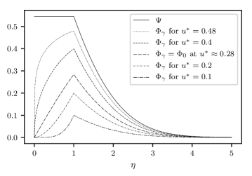
Figure 1. Plot of $\Psi$ and of the family of profiles $\Phi_{\gamma}$ for different precipitation thresholds $u^{*}$. The profiles in between $\Psi$ and $\Phi_{0}$ correspond to the transitional regime where $\gamma$ is negative, hence they fall outside of the class of self-similar solutions described by Theorem 7. Solutions to the HHMO-model in the transitional regime always converge to $\Phi_{0}$, not to $\Phi_{\gamma}$ with $\gamma<0$.

To proceed, we set

$$u^{*}_{\gamma}=\left(\frac{\kappa\,M\bigl{(}\frac{\kappa}{2}+1,\kappa+\frac{1}{2},-\frac{\alpha^{2}}{4}\bigr{)}}{\alpha\,M\bigl{(}\frac{\kappa}{2},\kappa+\frac{1}{2},-\frac{\alpha^{2}}{4}\bigr{)}}+\,\frac{\exp\bigl{(}-\frac{\alpha^{2}}{4}\bigr{)}}{\sqrt{\pi}\,\operatorname{erfc}(\frac{\alpha}{2})}\right)^{-1}\frac{\alpha\beta}{2}$$ (60)

and join the right-hand solution (47) and left-hand solution (50) to define a family of functions, parameterized by $\gamma$, by

$$\Phi_{\gamma}(\eta)=\begin{dcases}\frac{u^{*}_{\gamma}\,\eta^{\kappa}\,M\bigl{(}\frac{\kappa}{2},\kappa+\frac{1}{2},-\frac{\eta^{2}}{4}\bigr{)}}{\alpha^{\kappa}\,M\bigl{(}\frac{\kappa}{2},\kappa+\frac{1}{2},-\frac{\alpha^{2}}{4}\bigr{)}}&\text{ if }\eta<\alpha\,,\\ \frac{u^{*}_{\gamma}}{\operatorname{erfc}(\frac{\alpha}{2})}\,\operatorname{erfc}\Bigl{(}\frac{\eta}{2}\Bigr{)}&\text{ if }\eta\geq\alpha\,.\end{dcases}$$ (61)

For future reference, we note that in $x$-$t$ coordinates, this function takes the form

$$\phi_{\gamma}(x,t)=\Phi_{\gamma}(x/{\sqrt{t}})\,.$$ (62)

At this point, we know that each $\Phi_{\gamma}(\eta)$ satisfies the differential equation (41a) and the decay condition (41b). However, $\Phi_{\gamma}$ does not necessarily satisfy the internal boundary condition (41c), equivalent to the matching condition (59) which can now be expressed as $u^{*}_{\gamma}=u^{*}$, nor does it necessarily satisfy the Neumann boundary condition (41d), which requires $\gamma>0$ or, equivalently, $\kappa>1$. The following theorem states a necessary and sufficient condition such that (59) can be solved for $\kappa>1$ or, equivalently, $u^{*}_{\gamma}=u^{*}$ can be solved for $\gamma>0$. When this is the case, the resulting matched solution solves the entire system (41).

Theorem 7.

Let $\alpha$, $\beta$, and $u^{*}$ be positive. Then the matching condition $u^{*}_{\gamma}=u^{*}$ has a unique solution satisfying $\gamma>0$ if and only if $u^{*}<u_{0}^{*}$. If this is the case, the unique solution to (41) is given by (61) with this particular value of $\gamma$.

Remark 6.

We recall that for a subcritical precipitation threshold where $u^{*}>\Psi(\alpha)$, no precipitation can occur and $\Psi$, defined in (2), provides a self-similar solution without precipitation. The marginal case $u^{*}=\Psi(\alpha)$ is discussed in Theorem 5. In the transitional regime $u_{0}^{*}\leq u^{*}<\Psi(\alpha)$, there is some $\gamma\leq 0$ so that (61) still solves (41a–c); however, $\gamma<0$ is nonphysical and the Neumann condition (41d) cannot be satisfied in this regime. For future reference, we call the limiting case $u^{*}=u_{0}^{*}$ the critical precipitation threshold. In this case, (61) takes the form

$$\Phi_{0}(\eta)=\begin{dcases}\frac{u^{*}_{0}}{\operatorname{erf}(\frac{\alpha}{2})}\,\operatorname{erf}(\frac{\eta}{2})&\text{ if }\eta<\alpha\,,\\ \frac{u^{*}_{0}}{\operatorname{erfc}(\frac{\alpha}{2})}\,\operatorname{erfc}(\frac{\eta}{2})&\text{ if }\eta\geq\alpha\,.\end{dcases}$$ (63)

As discussed, this is not a solution, but will emerge as the universal asymptotic profile for solutions in the transitional regime. Finally, the supercritical regime $u^{*}<u_{0}^{*}$ is the regime where Theorem 7 provides a self-similar solution to the HHMO-model with self-similar precipitation function. The profiles for the different cases are summarized in Figure 1.

Proof of Theorem 7.

The form of the solution is determined by the preceding construction. It remains to show that when $u^{*}<u_{0}^{*}$, the derivative matching condition (59) has a unique solution $\kappa>1$. Let us consider the left-hand solution (50) as a function of $\eta$ and $\kappa$, which we denote by $v(\eta,\kappa)$, so that the leftmost term in (59) is $v_{\eta}(\alpha,\kappa)$.

We begin by noting that

$$v_{\eta}(\alpha,1)=u^{*}\,\frac{M\bigl{(}\frac{3}{2},\frac{3}{2},-\frac{\alpha^{2}}{4}\bigr{)}}{\alpha\,M\bigl{(}\frac{1}{2},\frac{3}{2},-\frac{\alpha^{2}}{4}\bigr{)}}\,.$$ (64)

Moreover,

$$\lim_{\kappa\to\infty}M\bigl{(}\tfrac{\kappa}{2}+1,\kappa+\tfrac{1}{2},-\tfrac{\alpha^{2}}{4}\bigr{)}=\lim_{\kappa\to\infty}M\bigl{(}\tfrac{\kappa}{2},\kappa+\tfrac{1}{2},-\tfrac{\alpha^{2}}{4}\bigr{)}=\exp\bigl{(}-\tfrac{\alpha^{2}}{8}\bigr{)}\,,$$ (65)

as is easily proved by using the dominated convergence theorem on the power series representation of Kummer’s function. Consequently, $v_{\eta}(\alpha,\kappa)$ grows without bound as $\kappa\to\infty$. Solvability under the condition that $u^{*}<u_{0}^{*}$ is then a simple consequence of the intermediate value theorem.

To prove uniqueness, we show that $v_{\eta}(\alpha,\kappa)$ is strictly monotonic in $\kappa$. For fixed $\kappa_{2}>\kappa_{1}$, we define

$$V(\eta)=v(\eta,\kappa_{2})-v(\eta,\kappa_{1})\,.$$ (66)

First, $v(\eta,\kappa_{1})$ and $v(\eta,\kappa_{2})$ satisfy the differential equation (49a) with respective constants $\gamma_{1}<\gamma_{2}$. Thus,

$$V^{\prime\prime}(\eta)+\frac{\eta}{2}\,V^{\prime}(\eta)=\frac{\gamma_{2}}{\eta^{2}}\,V(\eta)+\frac{\gamma_{2}-\gamma_{1}}{\eta^{2}}\,v(\eta,\kappa_{1})\,.$$ (67)

We note that $V(0)=V(\alpha)=0$. Assume that $V$ attains a local non-negative maximum at $\eta_{0}\in(0,\alpha)$. Then $V(\eta_{0})\geq 0$, $V^{\prime}(\eta_{0})=0$, and $V^{\prime\prime}(\eta_{0})\leq 0$. This contradicts (67) as the left hand side is non-positive and the right hand side is positive. We conclude that $V$ is negative in the interior of $[0,\alpha]$.

In particular, this means that $V^{\prime}(\alpha)\geq 0$. The proof is complete if we show that this inequality is strict. To proceed, assume the contrary, i.e., that $V^{\prime}(\alpha)=0$. However, inserting $V^{\prime}(\alpha)=V(\alpha)=0$ into (67), we see that there must exist a small left neighborhood of $\alpha$, $(\alpha_{0},\alpha)$ say, on which $V^{\prime\prime}$ is positive. This implies that $V^{\prime}$ is negative and $V$ is positive on $(\alpha_{0},\alpha)$, which is a contradiction. ∎

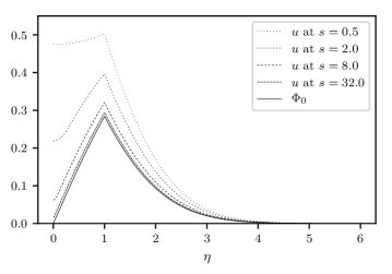
Figure 2. Plot of the function $u$ for $\alpha=1.0$, $\beta=1.0$ in the transitional regime with $u^{*}=0.49$ for different times $s$, together with the conjectured limit profile $\Phi_{0}$.

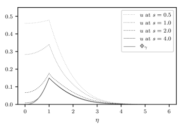
Figure 3. Plot of the function $u$ for $\alpha=1.0$, $\beta=1.0$ in the supercritical regime with $u^{*}=0.15$ for different times $s$, together with the conjectured limit profile $\Phi_{\gamma}$.

Figure 4. Longer-time diagnostics in the supercritical regime. Shown are two quantities on the line $\eta=\alpha$ relative to their conjectured limits for the simulation shown in Figure 3. The growing oscillations are an effect of the finite constant grid size, see text.

5. Numerical results

In the following, we present numerical evidence which suggests that the profiles $\Phi_{\gamma}$ derived in the previous section determine the long-time behavior of the solution to the HHMO-model. As the concentration is expected to converge uniformly in parabolic similarity coordinates, it is convenient to formulate the numerical scheme directly in $\eta$-$s$ coordinates. We use simple implicit first-order time-stepping for the concentration field and direct propagation of the precipitation function along its characteristic lines $x=\text{const}$ which transform to hyperbolic curves in the $\eta$-$s$ plane. Details of the scheme are provided in Appendix A.

The observed behavior is different in the transitional and in the supercritical regime. In the transitional regime, the source term is too weak to maintain precipitation outside of a bounded region on the $x$-axis, which transforms into a precipitation region which gets squeezed onto the $s$-axis as time progresses in $\eta$-$s$ coordinates. In this regime, the asymptotic profile is always $\Phi_{0}$; a particular example is shown in Figure 2. Note that the concentration peak drops well below the precipitation threshold as time progresses.

Figure 3 shows the long-time behavior of the concentration in the supercritical case. In this case, the limit profile is $\Phi_{\gamma}$, where $\gamma$ is determined as a function of $\alpha$, $\beta$, and $u^{*}$ by the solvability condition of Theorem 7. The convergence is very robust with respect to compactly supported changes in the initial condition (not shown). We note that the evolution equation in $\eta$-$s$ coordinates is singular at $s=0$, so the initial value problem is only well-defined when the initial condition is imposed at some $s_{0}>0$. For the numerical scheme, however, there is no problem initializing at $s=0$.

Along the line $\eta=\alpha$, equivalent to the parabola $t=x^{2}/\alpha^{2}$, on which the source point moves, the concentration is converging toward the critical concentration $u^{*}$. At the same time, the weighted average of the concentration,

$$h(x)=\frac{1}{x}\int_{0}^{x}\xi^{2}\,p^{*}(\xi)\,\mathrm{d}\xi\,,$$ (68)

is converging to $\gamma$ as $t\to\infty$ or, equivalently, $x\to\infty$. This behavior is clearly visible in Figure 4, where convergence in $h$ is much slower than convergence in $u$. Figure 4 also shows that grid effects become increasingly dominant as time progresses. This is due to the fact that precipitation occupies at least one full grid cell on the line $\eta=\alpha$. However, to be consistent with the conjectured asymptotics, the temporal width of the precipitation region needs to shrink to zero. In the discrete approximation, it cannot do this, resulting in oscillations of the diagnostics with increasing amplitude. For even larger times, the simulation eventually breaks down completely. This behavior can be seen as a manifestation of “rattling,” described by Gurevich and Tikhomirov [13, 14] in a related setting. Here, the scaling of the problem and of the computational domain leads to an increase of the rattling amplitude with time.

On any fixed finite interval of time, the amplitude of the grid oscillations vanishes as the spatial and temporal step sizes go to zero. However, it is impossible to design a code in which this behavior is uniform in time so long as the precipitation function takes only binary values, i.e., strictly follows condition (7).

6. Long-time behavior of a linear auxiliary problem

In this section, we study the nonautonomous linear system

$$u_{t}=u_{xx}+\frac{\alpha\beta}{2\sqrt{t}}\,\delta(x-\alpha\sqrt{t})-p\,u\,,$$ (69a)

$$u_{x}(0,t)=0\quad\text{for }t>0\,,$$ (69b)

$$u(x,0)=0\quad\text{for }x>0$$ (69c)

on the space-time domain $\mathbb{R}_{+}\times\mathbb{R}_{+}$. The equations coincide with the HHMO-model (3a–c). Here, however, we consider the precipitation function $p(x,t)$ as given, not necessarily related to $u$ in any way. The goal of this section is to give conditions on $p$ such that the solution $u$ converges uniformly in parabolic similarity coordinates to one of the profiles $\Phi_{\gamma}$ defined in Section 4.

Throughout, we assume that $p\in\mathcal{A}$, where

$$\mathcal{A}=\{p\in L^{1}_{\operatorname{loc}}((0,\infty)\times[0,\infty))\colon\\ \operatorname*{supp}p\cap(\mathbb{R}_{+}\times[0,T])\text{ is compact for every }T>0\}\,.$$ (70)

In addition, we will assume that $p$ is non-zero, non-negative, non-decreasing in time, and satisfies condition (P) stated in the introduction. In all of the following, we manipulate the equation formally as if the solution was strong. A detailed verification that all steps are indeed rigorous can be found in [6, Appendix B]; these result can be transformed into similarity variables as in Appendix B below. In this context, the condition on the support of $p$ in (70) eases the justification of the exchange of integration and time-differentiation. More generality is clearly possible, but this simple assumption covers all cases we need for the purpose of this paper.

For technical reasons, we distinguish two cases which require different treatment. In the first case, $p$ is assumed bounded. It is then easy to show that there exists a weak solution

$$u-\psi\in C^{1,0}(\mathbb{R}_{+}\times\mathbb{R}_{+})\cap L^{\infty}(\mathbb{R}_{+}\times\mathbb{R}_{+})\,,$$ (71)

satisfying (19), where $\psi$ is the solution of the precipitation-less equation given by (2); see, e.g., [6, Appendix B].

In the second case, $p$ may be unbounded. In general, the existence of solutions is then not obvious, so that we assume a solution with

$$u-\psi\in C^{1,0}(\mathbb{R}_{+}\times\mathbb{R}_{+})\cap W^{1,1}_{2,{\operatorname{loc}}}(\mathbb{R}_{+}\times\mathbb{R}_{+})$$ (72)

exists, and that this solution satisfies the bound

$$0\leq u\leq\phi_{0}\quad\text{provided}\quad\int_{0}^{\infty}p^{*}(x)\,\mathrm{d}x=\infty$$ (73)

with $\phi_{0}$ given by (62), or

$$0\leq u\leq\psi\quad\text{provided}\quad\int_{0}^{\infty}p^{*}(x)\,\mathrm{d}x<\infty\,.$$ (74)

We remark that when $p$ is bounded, it is easy to prove that solutions $u$ which decay as $x\to\infty$ satisfy the weaker bound (74).

Remark 7.

Here we will explain why we impose (73). Proceeding formally, we fix $0<t_{0}<t_{1}$ and $0<x_{1}<\alpha\sqrt{t_{0}}$, multiply (69a) by $u$, integrate over $[0,x_{1}]\times[t_{0},t_{1}]$, and note that the domain of integration is away from the location of the source, so that

$$\int_{0}^{x_{1}}u^{2}\,\mathrm{d}x\bigg{|}^{t=t_{1}}_{t=t_{0}} =2\int_{t_{1}}^{t_{2}}u_{x}\,u\,\mathrm{d}t\bigg{|}_{x=0}^{x=x_{1}}$$

$$\quad-2\int_{t_{0}}^{t_{1}}\int_{0}^{x_{1}}u_{x}^{2}\,\mathrm{d}x\,\mathrm{d}t-2\int_{0}^{x_{1}}p^{*}(x)\int_{t_{0}}^{t_{1}}u^{2}\,\mathrm{d}t\,\mathrm{d}x\,.$$ (75)

As $u$ and $u_{x}$ are continuous on the domain of integration, the first three integrals are finite. Thus, the last integral must be finite, too. When $p^{*}$ is not integrable near zero, this can only be true when $u(0,t)=0$ for all $t>0$. Now note that $\phi_{0}$ satisfies (69a) for $p\equiv 0$ with Dirichlet boundary conditions

$$\phi_{0}(0,t)=0\quad\text{for }t>0\,,$$

$$\phi_{0}(x,0)=\lim_{\begin{subarray}{c}y\to x\\ t\searrow 0\end{subarray}}\phi_{0}(y,t)=0\quad\text{for }x>0\,,$$

Thus, $\phi_{0}$ is the natural supersolution for $u$ when $p^{*}$ is not integrable.

Lemma 8.

Let $p\in\mathcal{A}$ be non-negative and non-decreasing in time $t$. Let $u$ be a weak solution to (69). Then $u-\psi$ is non-increasing in time $t$.

Proof.

The proof of [17, Lemma 3.3] applies literally. We remark that the result in [17] is stated for solutions to the HHMO-model, but its proof depends only on the assumption that $p$ is non-decreasing in $t$ and applies here as well. ∎

Lemma 9.

Suppose $p\in\mathcal{A}$ is non-zero, nonnegative, and satisfies condition (P). Let $u$ be a weak solution to (69). Then $u(0,t)\to 0$ as $t\to\infty$.

Remark 8.

This lemma can be applied to weak solutions of the HHMO-model (3) provided $u^{*}<\Psi(\alpha)$ under the additional assumption that (10) is satisfied. Then, by [17, Lemma 3.5], there is at least one non-degenerate precipitation region and the assumptions of the lemma apply.

Proof.

We construct a supersolution to $u$ as follows. Fix any $y^{*}>0$ such that the support of $p^{*}$ intersects $[0,y^{*}]$ on a set of positive measure. Define $t^{*}=(y^{*}/\alpha)^{2}$ and

$$p^{r}(x,t)=\begin{cases}\min\{p^{*}(\lvert x\rvert),1\}&\text{if }x\in[-y^{*},y^{*}]\text{ and }t\geq x^{2}/\alpha^{2}\,,\\ 0&\text{otherwise}\,.\\ \end{cases}$$ (77)

Let $u^{r}$ denote the unique bounded weak solution to (69) with $p=p^{r}$ and extend $u^{r}$ to the left half-plane by even reflection. Due to the subsolution principle, $0\leq u\leq u^{r}$. Our goal is to show that $u^{r}(0,t)\to 0$ as $t\to\infty$. We reflect $u^{r}$ evenly with respect to $x=0$ axis. Note that $p^{r}$ fulfills the conditions of Lemma 8. Therefore, $u^{r}$ is non-increasing in $t$ on $[-y^{*},y^{*}]\times[t^{*},\infty)$ so that

$$\lim_{t\to\infty}\inf_{x\in[-y^{*},y^{*}]}u^{r}(x,t)\equiv c$$ (78)

exists. We now express $u^{r}(0,t)$ for $t>t^{*}$ via the Duhamel formula, bound $u^{r}$ from below by $c$, note that $K(-y,t-s)$ is a decreasing function in $y$, and recall that $p^{r}$ is supported on $\{\tau\geq t^{*}\}$ to estimate

$$u^{r}(0,t) =\psi(0,t)-\int_{0}^{t}\int_{-y^{*}}^{y^{*}}K(-y,t-\tau)\,p^{r}(y)\,u^{r}(y,\tau)\,\mathrm{d}y\,\mathrm{d}\tau$$

$$\leq\Psi(0)-c\int_{-y^{*}}^{y^{*}}p^{r}(y)\,\mathrm{d}y\int_{t^{*}}^{t}K(y^{*},t-\tau)\,\mathrm{d}\tau\,.$$ (79)

Changing variables $\tau\to t\tau^{\prime}$ in the second integral on the right, we find that

$$\int_{t^{*}}^{t}K(y^{*},t-\tau)\,\mathrm{d}\tau =\sqrt{t}\int_{t^{*}/t}^{1}\frac{1}{\sqrt{4\pi(1-\tau^{\prime})}}\,\mathrm{e}^{-\tfrac{{y^{*}}^{2}}{4t(1-\tau^{\prime})}}\,\mathrm{d}\tau^{\prime}$$

$$\sim\sqrt{t}\int_{0}^{1}\frac{1}{\sqrt{4\pi(1-\tau^{\prime})}}\,\mathrm{d}\tau^{\prime}=\sqrt{\frac{t}{\pi}}$$ (80)

as $t\to\infty$. This implies $c=0$ as otherwise $u^{r}(0,t)\to-\infty$ as $t\to\infty$. Then the Harnack inequality for the function $u^{r}$ on some spatial domain containing the interval $[-y^{*},y^{*}]$ implies that for any fixed $\delta>0$ there exists a constant $C_{\delta}>0$ such that

$$u^{r}(0,t)\leq\sup_{y\in[-y^{*},y^{*}]}u^{r}(y,t)\leq C_{\delta}\,\inf_{y\in[-y^{*},y^{*}]}u^{r}(y,t+\delta)\to 0\text{ as }t\to\infty\,;$$ (81)

see, e.g., [11, Section 7.1.4.b] and [24]. Hence, $u(0,t)\to 0$ as well. ∎

Lemma 10.

Let $p\in\mathcal{A}$ be non-negative and non-decreasing in time $t$. Let $u$ a bounded weak solution to (69) where, as before, we write $u(x,t)=v(x/\sqrt{t},\sqrt{t})$. Then for every $d>0$ and $\gamma\geq 0$, the following is true.

1. There exists $\omega\in(0,1)$ such that for every $(\eta,s)$ with $v(\eta,s)-\Phi_{\gamma}(\eta)\geq d$,

   $$\min_{s^{\prime}\in[\omega s,s]}\max_{\eta\in\mathbb{R}_{+}}\{v(\eta,s^{\prime})-\Phi_{\gamma}(\eta)\}\geq d/2\,.$$ (82)

2. There exists $\omega\in(1,\infty)$ such that for every $(\eta,s)$ with $v(\eta,s)-\Phi_{\gamma}(\eta)\leq-d$,

   $$\max_{s^{\prime}\in[s,\omega s]}\min_{\eta\in\mathbb{R}_{+}}\{v(\eta,s^{\prime})-\Phi_{\gamma}(\eta)\}\leq-d/2\,.$$ (83)

Proof.

Set $V(\eta)=\Psi(\eta)-\Phi_{\gamma}(\eta)$. By direct inspection, we see that $V$ is strictly decreasing on $\mathbb{R}_{+}$. In case (a),

$$d\leq v(\eta,s)-\Phi_{\gamma}(\eta)\leq V(\eta)\,.$$ (84)

Therefore, the possible values of $\eta$ for which the assumption of case (a) can be satisfied are bounded from above by some $\eta^{*}=\eta^{*}(d,\gamma)$. By the mean value theorem, for $\omega\in(0,1)$,

$$V(\eta)-V(\eta/\omega)\leq\max_{\xi\in[\eta,\eta/\omega]}\lvert V^{\prime}(\xi)\rvert\,\Bigl{(}\frac{\eta}{\omega}-\eta\Bigr{)}\leq\eta^{*}\,\max_{\xi\in[0,\eta^{*}/\omega]}\lvert V^{\prime}(\xi)\rvert\,\frac{1-\omega}{\omega}\leq\frac{d}{2}$$ (85)

where, in the last inequality, $\omega$ has been fixed sufficiently close to $1$. This choice is independent of $\eta$. Now recall that $t=s^{2}$ and $x=\eta s$. Choose any $s^{\prime}\in[\omega s,s]$, set $t^{\prime}={s^{\prime}}{\vphantom{s}}^{2}$ and $\eta^{\prime}=x/s^{\prime}$ so that $\eta^{\prime}\leq\eta/\omega$. Then

$$d-(u(x,t^{\prime})-\phi_{\gamma}(x,t^{\prime})) \leq(u(x,t)-\phi_{\gamma}(x,t))-(u(x,t^{\prime})-\phi_{\gamma}(x,t^{\prime}))$$

$$=(u(x,t)-\psi(x,t))-(u(x,t^{\prime})-\psi(x,t^{\prime}))+V(\eta)-V(\eta^{\prime})$$

$$\leq V(\eta)-V(\eta/\omega)\leq d/2\,,$$ (86)

where the first inequality is due to the assumption of case (a), the second inequality is due to Lemma 8 which states that $u-\psi$ is non-increasing in $t$ for $x$ fixed. We further used monotonicity of $V$ in the second inequality. The last inequality is due to (85). Altogether, we see that

$$v(\eta^{\prime},s^{\prime})-\Phi_{\gamma}(\eta^{\prime})=u(x,t^{\prime})-\phi_{\gamma}(x,t^{\prime})\geq d/2\,.$$ (87)

This proves (82). The proof in case (b) is similar. Notice that

$$v(\eta,s)\leq\Phi_{\gamma}(\eta)-d<\Phi_{\gamma}(\eta).$$ (88)

Therefore, the possible values of $\eta$ for which the assumption of case (b) can be satisfied are bounded from below by some $\eta^{*}=\eta^{*}(d,\gamma)>0$. The rest of the proof is obvious. ∎

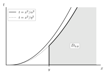
Figure 5. Sketch of the region $D_{\eta,y}$ when $\eta>\alpha$.

In the following, for positive real numbers $\eta$, $y$, and $T$, we define

$$D_{\eta,y}=\{(x,t)\colon x\geq y,0\leq t\leq\eta^{-2}x^{2}\}\,.$$ (89)

See Figure 5 for an illustration.

Theorem 11.

Let $p\in\mathcal{A}$ be non-zero, non-negative, non-decreasing in time, and satisfy condition (P). Assume further for each $\eta>\alpha$ there exists $y=y(\eta)$ such that $p\equiv 0$ on $D_{\eta,y}$, and that there exists $\gamma\geq 0$ such that

$$\lim_{x\to\infty}x\int^{\infty}_{x}p^{*}(\xi)\,\mathrm{d}\xi=\gamma\,,$$ (90)

where $p^{*}$ denotes the values of $p$ along the line $\eta=\alpha$ as defined in condition (P).

Let $u$ be a weak solution of class (71) to the linear non-autonomous equation (69) with $p$ fixed as stated. If $p$ is unbounded, assume further that $u$ is of class (72) and satisfies the bounds (73) or (74). Then $u$ converges uniformly to $\Phi_{\gamma}$.

Proof.

Set $w=v-\Phi_{\gamma}$. Subtracting (41a) from (13a) and noting that, by assumption, $q(\eta,s)=p^{*}(s\eta)$ for $\eta<\alpha$, we obtain

$$\tfrac{1}{2}\,s\,w_{s}-\tfrac{1}{2}\,\eta\,w_{\eta}=w_{\eta\eta}-s^{2}\,q(\eta,s)\,w\\ +\Bigl{(}\frac{\gamma}{\eta^{2}}-s^{2}\,p^{*}(s\eta)\Bigr{)}\,\Phi_{\gamma}\,H(\alpha-\eta)-s^{2}\,q(\eta,s)\,\Phi_{\gamma}\,H(\eta-\alpha)$$ (91a)

with assumed bounds on $$w$$, namely

$$-\Phi_{\gamma}\leq w\leq\Phi_{0}-\Phi_{\gamma}\quad\text{provided}\quad\int_{0}^{\infty}p^{*}(x)\,\mathrm{d}x=\infty$$ (91b)

or

$$-\Phi_{\gamma}\leq w\leq\Psi-\Phi_{\gamma}\quad\text{provided}\quad\int_{0}^{\infty}p^{*}(x)\,\mathrm{d}x<\infty\,.$$ (91c)

To avoid boundary terms when integrating by parts, we introduce a fourth-power function with cut-off near zero which is defined, for every $\varepsilon>0$, by

$$J_{\varepsilon}(z)=\begin{cases}0&\text{if }|z|<\varepsilon\,,\\ (|z|-\varepsilon)^{4}&\text{if }|z|\geq\varepsilon\,.\end{cases}$$ (92)

$J_{\varepsilon}$ is at least twice continuously differentiable, even, positive, and strictly convex on $(\varepsilon,\infty)$. We now consider the cases when $p^{*}$ is integrable and $p^{*}$ is not integrable separately.

Case 1 ($p^{*}$ is not integrable on $\mathbb{R}_{+}$).

In this case, we have the bound (91b), so that $|w|\leq\Phi_{0}+\Phi_{\gamma}$. Hence, for $\varepsilon>0$, arbitrary but fixed in the following, there are $\eta_{0}=\eta_{0}(\varepsilon)$ and $\eta_{1}=\eta_{1}(\varepsilon)$ with $0<\eta_{0}<\eta_{1}<\infty$ such that $|w|\leq\varepsilon$, hence $J_{\varepsilon}(w)=0$, for $\eta\notin(\eta_{0},\eta_{1})$ and all $s>0$.

We multiply (91a) by $J_{\varepsilon}^{\prime}(w)$, integrate on $\mathbb{R}_{+}$, and examine the resulting expression term-by-term. The contribution from the first term reads

$$\frac{1}{2}\int_{0}^{\infty}s\,w_{s}\,J^{\prime}_{\varepsilon}(w)\,\mathrm{d}\eta=\frac{s}{2}\,\frac{\mathrm{d}}{\mathrm{d}s}\int_{\eta_{0}}^{\infty}J_{\varepsilon}(w)\,\mathrm{d}\eta$$ (93)

and the second term contributes

$$\frac{1}{2}\int_{0}^{\infty}\eta\,w_{\eta}\,J^{\prime}_{\varepsilon}(w)\,\mathrm{d}\eta =\frac{1}{2}\int_{\eta_{0}}^{\eta_{1}}\eta\,w_{\eta}\,J^{\prime}_{\varepsilon}(w)\,\mathrm{d}\eta$$

$$=-\frac{1}{2}\int_{\eta_{0}}^{\eta_{1}}J_{\varepsilon}(w)\,\mathrm{d}\eta=-\frac{1}{2}\int_{\eta_{0}}^{\infty}J_{\varepsilon}(w)\,\mathrm{d}\eta\,.$$ (94)

Combining both expressions, we obtain

$$\frac{s}{2}\,\frac{\mathrm{d}}{\mathrm{d}s}\int_{\eta_{0}}^{\infty}J_{\varepsilon}(w)\,\mathrm{d}\eta+\frac{1}{2}\int_{\eta_{0}}^{\infty}J_{\varepsilon}(w)\,\mathrm{d}\eta=\frac{\mathrm{d}}{\mathrm{d}s}\biggl{(}\frac{s}{2}\int_{\eta_{0}}^{\infty}J_{\varepsilon}(w)\,\mathrm{d}\eta\biggr{)}\,.$$ (95)

The contribution from the first term on the right of (91a) reads

$$\int_{0}^{\infty}w_{\eta\eta}\,J^{\prime}_{\varepsilon}(w)\,\mathrm{d}\eta =\int_{\eta_{0}}^{\eta_{1}}w_{\eta\eta}\,J^{\prime}_{\varepsilon}(w)\,\mathrm{d}\eta$$

$$=-\int_{\eta_{0}}^{\eta_{1}}w_{\eta}^{2}\,J^{\prime\prime}_{\varepsilon}(w)\,\mathrm{d}\eta=-\int_{\eta_{0}}^{\infty}w_{\eta}^{2}\,J^{\prime\prime}_{\varepsilon}(w)\,\mathrm{d}\eta\,.$$ (96)

The contribution from the second term on the right of (91a) satisfies

$$-\int_{0}^{\infty}s^{2}\,q(\eta,s)\,w\,J^{\prime}_{\varepsilon}(w)\,\mathrm{d}\eta\leq 0$$ (97)

because the product $w\,J^{\prime}_{\varepsilon}(w)$ is clearly non-negative. To investigate the contribution coming from the third term on the right of (91a), we integrate by parts, so that

$$\int_{0}^{\infty}\Bigl{(}\frac{\gamma}{\eta^{2}}-s^{2}\,p^{*}(s\eta)\Bigr{)}\,\Phi_{\gamma}\,H(\alpha-\eta)\,J^{\prime}_{\varepsilon}(w)\,\mathrm{d}\eta$$

$$=\int_{\eta_{0}}^{\alpha}\Bigl{(}\frac{\gamma}{\eta^{2}}-s^{2}\,p^{*}(s\eta)\Bigr{)}\,\Phi_{\gamma}\,J^{\prime}_{\varepsilon}(w)\,\mathrm{d}\eta$$

$$=g(\alpha,s)\,\Phi_{\gamma}(\alpha)\,J^{\prime}_{\varepsilon}(w(\alpha,s))-\int_{\eta_{0}}^{\alpha}g\,\Phi^{\prime}_{\gamma}\,J^{\prime}_{\varepsilon}(w)\,\mathrm{d}\eta-\int_{\eta_{0}}^{\alpha}g\,\Phi_{\gamma}\,w_{\eta}\,J^{\prime\prime}_{\varepsilon}(w)\,\mathrm{d}\eta\,,$$ (98)

where $g$ is an anti-derivative of the term in parentheses, namely

$$g(\eta,s)=s^{2}\int_{\eta}^{\infty}p^{*}(s\kappa)\,\mathrm{d}\kappa-\frac{\gamma}{\eta}=s\int_{s\eta}^{\infty}p^{*}(\zeta)\,\mathrm{d}\zeta-\frac{\gamma}{\eta}\,.$$ (99)

We note that for fixed $\eta>0$, due to (90), $g(\eta,s)\to 0$ as $s\to\infty$.

When $\varepsilon<u^{*}$, the equation $\Phi_{0}(\eta)=\varepsilon$ has one root $\eta\leq\alpha$. Since $u\leq\Phi_{0}$, we can set $\eta_{0}=\eta$ so that $\eta_{0}\leq\alpha$, which we assume henceforth. Combining (96) with the last term in (98), we obtain

$$-\int_{\eta_{0}}^{\infty} w_{\eta}^{2}\,J^{\prime\prime}_{\varepsilon}(w)\,\mathrm{d}\eta-\int_{\eta_{0}}^{\alpha}g\,\Phi_{\gamma}\,w_{\eta}\,J^{\prime\prime}_{\varepsilon}(w)\,\mathrm{d}\eta$$

$$=-\int_{\alpha}^{\infty}w_{\eta}^{2}\,J^{\prime\prime}_{\varepsilon}(w)\,\mathrm{d}\eta-\int_{\eta_{0}}^{\alpha}\bigl{(}w_{\eta}+\tfrac{1}{2}\,g\,\Phi_{\gamma}\bigr{)}^{2}\,J^{\prime\prime}_{\varepsilon}(w)\,\mathrm{d}\eta$$

$$\quad+\frac{1}{4}\int_{\eta_{0}}^{\alpha}g^{2}\,\Phi_{\gamma}^{2}\,J^{\prime\prime}_{\varepsilon}(w)\,\mathrm{d}\eta$$

$$=\frac{1}{2}\int_{\eta_{0}}^{\alpha}g^{2}\,\Phi_{\gamma}^{2}\,J^{\prime\prime}_{\varepsilon}(w)\,\mathrm{d}\eta-G^{*}(s)$$ (100)

where

$$G^{*}(s) =\int_{\alpha}^{\infty}w_{\eta}^{2}\,J^{\prime\prime}_{\varepsilon}(w)\,\mathrm{d}\eta+\int_{\eta_{0}}^{\alpha}\bigl{(}w_{\eta}+\tfrac{1}{2}\,g\,\Phi_{\gamma}\bigr{)}^{2}\,J^{\prime\prime}_{\varepsilon}(w)\,\mathrm{d}\eta+\frac{1}{4}\int_{\eta_{0}}^{\alpha}g^{2}\,\Phi_{\gamma}^{2}\,J^{\prime\prime}_{\varepsilon}(w)\,\mathrm{d}\eta$$

$$\geq\int_{\alpha}^{\infty}w_{\eta}^{2}\,J^{\prime\prime}_{\varepsilon}(w)\,\mathrm{d}\eta+\frac{1}{2}\int_{\eta_{0}}^{\alpha}w_{\eta}^{2}\,J^{\prime\prime}_{\varepsilon}(w)\,\mathrm{d}\eta$$

$$\geq\frac{1}{2}\int_{0}^{\infty}w_{\eta}^{2}\,J^{\prime\prime}_{\varepsilon}(w)\,\mathrm{d}\eta\,.$$ (101)

We note that we have used the Jensen inequality in the first inequality of this lower bound estimate.

Finally, the last term on the right of (91a) is treated as follows. We define

$$F(s)=s^{2}\int_{0}^{\infty}q(\eta,s)\,\Phi_{\gamma}\,J_{\varepsilon}^{\prime}(w)\,H(\eta-\alpha)\,\mathrm{d}\eta$$ (102)

and

$$\Gamma(x)=x\int_{x}^{\infty}p^{*}(\xi)\,\mathrm{d}\xi\,.$$ (103)

For fixed $\eta^{*}>\alpha$ we can find $y=y(\eta^{*})$ such that $p\equiv 0$ on $D_{\eta^{*},y}$, i.e., $q(\eta,s)=0$ for all $\eta>\eta^{*}$ and $s\geq y/\eta^{*}$.

Then, for $s\geq s_{0}\equiv y/\eta^{*}$,

$$F(s)\leq\Phi_{\gamma}(\alpha)\,J_{\varepsilon}^{\prime}(\Psi(\alpha))\int_{\alpha}^{\eta^{*}}s^{2}\,q(\eta,s)\,\mathrm{d}\eta\,.$$ (104)

Since $p$ is non-decreasing in time $t$, we estimate

$$\int_{\alpha}^{\eta^{*}}s^{2}\,q(\eta,s)\,\mathrm{d}\eta\leq\int_{\alpha}^{\eta^{*}}s^{2}\,p^{*}(\eta s)\,\mathrm{d}\eta=s\int_{s\alpha}^{s\eta^{*}}p^{*}(\kappa)\,\mathrm{d}\kappa=\frac{\Gamma(s\alpha)}{\alpha}-\frac{\Gamma(s\eta^{*})}{\eta^{*}}\,.$$ (105)

Inserting this bound into (104) and noting that, due to (90), $\lim_{x\to\infty}\Gamma(x)=\gamma$, we find that

$$\limsup_{s\to\infty}F(s)\leq\Phi_{\gamma}(\alpha)\,J_{\varepsilon}^{\prime}(\Psi(\alpha))\,\Bigl{(}\frac{\gamma}{\alpha}-\frac{\gamma}{\eta^{*}}\Bigr{)}\,.$$ (106)

Adding up the individual contributions and neglecting the clearly non-positive terms on the right hand side as indicated, we obtain altogether

$$\frac{\mathrm{d}}{\mathrm{d}s}\biggl{(}\frac{s}{2}\int_{0}^{\infty}J_{\varepsilon}(w)\,\mathrm{d}\eta\biggr{)}\leq G(s)-G^{*}(s)+F(s)$$ (107)

with

$$G(s)=g(\alpha,s)\,\Phi_{\gamma}(\alpha)\,J^{\prime}_{\varepsilon}(w(\alpha,s))-\int_{\eta_{0}}^{\alpha}g\,\Phi^{\prime}_{\gamma}J^{\prime}_{\varepsilon}(w)\,\mathrm{d}\eta+\frac{1}{2}\int_{\eta_{0}}^{\alpha}g^{2}\,\Phi_{\gamma}^{2}\,J^{\prime\prime}_{\varepsilon}(w)\,\mathrm{d}\eta\,.$$ (108)

We note that $G(s)\to 0$ as $s\to 0$. Indeed, the first term converges to zero because $g$ converges to zero. The two integrals converge to zero because, in addition, on $[\eta_{0},\alpha]$ the function $g$ satisfies the uniform bound

$$g(\eta,s)=\frac{\Gamma(\eta s)-\gamma}{\eta}\leq\frac{1}{\eta}\,\sup_{x\geq\eta_{0}s_{0}}\Gamma(x)$$ (109)

which, together with the known bounds on $\Phi$, $\Phi^{\prime}$, and $w$, implies that the dominated convergence theorem is applicable. Hence, each of the integrals converges to zero.

Integrating (107) from $s_{0}$ to $s$, we obtain

$$\int_{0}^{\infty}J_{\varepsilon}(w(\eta,s))\,\mathrm{d}\eta-\frac{s_{0}}{s}\int_{0}^{\infty}J_{\varepsilon}(w(\eta,s_{0})\,\mathrm{d}\eta\leq\frac{2}{s}\int_{s_{0}}^{s}\bigl{(}G(\sigma)-G^{*}(\sigma)+F(\sigma)\bigr{)}\,\mathrm{d}\sigma\,.$$ (110)

We now take $\limsup_{s\to\infty}$. The second term on the left vanishes trivially. Since $G$ converges to zero, so does its time average, so its contribution is negligible in the limit. $G^{*}$ is non-negative, hence can be neglected. For the contribution from $F$, we refer to (106). Hence,

$$\limsup_{s\to+\infty}\int_{0}^{\infty}J_{\varepsilon}(w)\,\mathrm{d}\eta\leq 2\Phi_{\gamma}(\alpha)\,J_{\varepsilon}^{\prime}(\Psi(\alpha))\,\Bigl{(}\frac{\gamma}{\alpha}-\frac{\gamma}{\eta^{*}}\Bigr{)}\,.$$ (111)

Since $\eta^{*}>\alpha$ is arbitrary, we conclude that

$$\lim_{s\to\infty}\int_{0}^{\infty}J_{\varepsilon}(w(\eta,s))\,\mathrm{d}\eta=0\,.$$ (112)

This implies that for every fixed $\varepsilon>0$,

$$m(\{\eta\colon\lvert w\rvert>2\varepsilon\})\,J_{\varepsilon}(2\varepsilon)\leq\int_{\{\eta\colon\lvert w\rvert>2\varepsilon\}}J_{\varepsilon}(w)\,\mathrm{d}\eta\leq\int_{0}^{\infty}J_{\varepsilon}(w)\,\mathrm{d}\eta\to 0$$ (113)

as $s\to\infty$, where $m$ is the Lebesgue measure on the real line, i.e., $\lvert w\rvert$ converges to zero in measure. Due to the bound on $w$, the dominated convergence theorem with convergence in measure, e.g. [4, Corollary 2.8.6], implies that $v\to\Phi_{\gamma}$ in $L^{r}(\mathbb{R}_{+})$ for every $r\in[1,\infty)$.

Case 2 ($p^{*}$ is integrable on $\mathbb{R}_{+}$).

When $p^{*}$ is integrable, we only have the weaker bound on $w$ given by (91c). Thus, we must take $\eta_{0}=0$. On the other hand, due to Lemma 9, $u(0,s)$ is converging to $0$ as $s\to\infty$. Thus, we fix $\varepsilon>0$ and choose $s_{0}=s_{0}(\varepsilon)$ satisfying $u(0,s_{0})<\varepsilon$. Then $J_{\varepsilon}(w(0,s))=J_{\varepsilon}^{\prime}(w(0,s))=0$ for all $s>s_{0}$ so that the boundary terms when iterating by parts in (96), (94), and (98) vanish as before, so that all computations from Case 1 up to equation (108) remain valid as before.

The bound on $g$ now takes the form

$$g(\eta,s)=\frac{\Gamma(\eta s)-\gamma}{\eta}\leq\frac{1}{\eta}\,\sup_{x\geq 0}\Gamma(x)$$ (114)

where, as before, $\Gamma$ is given by (103). This implies that the integrands in the second and third term in (108) satisfy bounds on the interval $[0,\alpha]$ which take the form

$$\lvert g\,\Phi^{\prime}_{\gamma}\,J^{\prime}_{\varepsilon}(w)\rvert\leq C_{1}\,\eta^{\kappa-2}\,,$$ (115a)

$$\lvert g^{2}\,\Phi_{\gamma}^{2}\,J^{\prime\prime}_{\varepsilon}(w)\rvert\leq C_{2}\,\eta^{2(\kappa-1)}\,,$$ (115b)

where $C_{1}$ and $C_{2}$ are positive constants. When $\gamma>0$ so that $\kappa>1$, both bounds are integrable on $[0,\alpha]$ and the dominated convergence theorem applies as before, proving that $G(s)\to 0$ as $s\to\infty$. When $\gamma=0$ so that $\kappa=1$, the second bound (115b) is still integrable, but the first is not. Thus, for the second term on the right of (108), we change the strategy as follows.

Observe that when $\gamma=0$, then

$$g(\eta,s)=s\int_{s\eta}^{\infty}p^{*}(\zeta)\,\mathrm{d}\zeta\geq 0\,.$$ (116)

Thus, the second term in (108) is bounded above by

$$-\int_{0}^{\alpha}g(\eta,s)\,\Phi_{0}^{\prime}(\eta)\,J_{\varepsilon}^{\prime}(w(\eta,s))\,\mathrm{d}\eta\leq\int_{0}^{\alpha}\mathbb{I}_{\{w(\eta,s)<0\}}(\eta)\,g(\eta,s)\,\Phi_{0}^{\prime}(\eta)\,\lvert J_{\varepsilon}^{\prime}(w(\eta,s))\rvert\,\mathrm{d}\eta\,.$$ (117)

Note that $w(\eta,s)<0$ if and only if $u(\eta,s)<\Phi_{0}(\eta)$. Moreover, $\Phi_{0}(\eta)=O(\eta)$ as $\eta\to 0$ so that $\mathbb{I}_{\{w<0\}}\,J_{\varepsilon}^{\prime}(w)=O(\eta^{3})$. Altogether, there exists $C_{3}>0$ such that

$$\mathbb{I}_{\{w(\eta,s)<0\}}(\eta)\,g(\eta,s)\,\Phi_{0}^{\prime}(\eta)\,\lvert J_{\varepsilon}^{\prime}(w(\eta,s))\rvert\leq C_{3}\,\eta^{2}$$ (118)

which provides an integrable upper bound for the integrand on the right of (117). The dominated convergence theorem then proves that the integral on the right of (117) converges to zero as $s\to\infty$.

Thus, we find in all cases that $\limsup_{\sigma\to\infty}G(\sigma)\leq 0$, so that the argument from (110) to (112) proceeds as before and (113) is valid for every $\varepsilon>0$. This shows that $\lim_{s\to\infty}w=0$ in $L^{r}$.

In the final step, we bootstrap from $L^{r}$-convergence to uniform convergence on $\mathbb{R}_{+}$. We argue by contradiction and for both cases at once.

Suppose convergence is not uniform. Then there exists $d>0$ such that

$$\limsup_{s\to\infty}\max_{\eta\in\mathbb{R}_{+}}w(\eta,s)\geq 2d$$ (119)

or

$$\liminf_{s\to\infty}\min_{\eta\in\mathbb{R}_{+}}w(\eta,s)\leq-2d\,.$$ (120)

Suppose that the first alternative holds; the argument for the second alternative proceeds analogously and shall be omitted. By Lemma 10(a), there exists $\omega\in(0,1)$, a sequence $s_{i}\to\infty$, and a sequence $\eta_{i}$ such that for every $i\in\mathbb{N}$,

$$\min_{s\in[\omega s_{i},s_{i}]}w(\eta_{i},s)\geq d/2\,.$$ (121)

Due to the uniform bound on $w$ which decays as $\eta\to\infty$, the sequence $\eta_{i}$ must be contained in a compact interval of length $L$ (possibly dependent on $d$). In the following, fix $\varepsilon<d/4$.

For fixed $s\in[\omega s_{i},s_{i}]$, let

$$\eta_{0}=\max\{\eta<\eta_{i}\colon J_{\varepsilon}(w(\eta,s))=0\}\,.$$ (122)

(By continuity, the maximum exists and is less than $\eta_{i}$; in Case 2 we may need to take $i$ large enough so that $\omega s_{i}>s_{0}$.) Due to the fundamental theorem of calculus,

$$J_{\varepsilon}^{1/2}(w(\eta_{i},s))-J_{\varepsilon}^{1/2}(w(\eta_{0},s))=\int_{\eta_{0}}^{\eta_{i}}\partial_{\eta}J_{\varepsilon}^{1/2}(w(\eta,s))\,\mathrm{d}\eta$$ (123)

so that, noting that $J_{\varepsilon}^{1/2}(w(\eta_{i},s))=0$, $J_{\varepsilon}^{1/2}(w(\eta_{0},s))\geq(d/2-\varepsilon)^{2}$, and $d/2-\varepsilon\geq d/4$ on the left and using the Cauchy–Schwarz inequality on the right, we obtain

$$\Bigl{(}\frac{d}{4}\Bigr{)}^{2}\leq(\eta_{i}-\eta_{0})^{\tfrac{1}{2}}\,\biggl{(}\int_{\eta_{0}}^{\eta_{i}}4\,(\lvert w\rvert-\varepsilon)^{2}\,w_{\eta}^{2}\,\mathrm{d}\eta\biggr{)}^{\tfrac{1}{2}}\leq\sqrt{L}\,\biggl{(}\frac{1}{3}\int_{\mathbb{R}_{+}}J_{\varepsilon}^{\prime\prime}(w)\,w_{\eta}^{2}\,\mathrm{d}\eta\biggr{)}^{\tfrac{1}{2}}\,.$$ (124)

We conclude that the integral on the right is bounded below by some strictly positive constant, say $b$, which only depends on $d$. Due to (101), $b/2$ is also a lower bound on $G^{*}$. Thus, returning to (110) with $s=s_{i}$ and $s_{0}=\omega s_{i}$, we obtain

$$\int_{0}^{\infty}J_{\varepsilon}(w(\eta,s_{i}))\,\mathrm{d}\eta -\omega\int_{0}^{\infty}J_{\varepsilon}(w(\eta,\omega s_{i})\,\mathrm{d}\eta\leq\frac{2}{s_{i}}\int_{\omega s_{i}}^{s_{i}}\bigl{(}G(\sigma)-G^{*}(\sigma)+F(\sigma)\bigr{)}\,\mathrm{d}\sigma$$

$$\leq-(1-\omega)\,b+\frac{2}{s_{i}}\int_{\omega s_{i}}^{s_{i}}\bigl{(}G(\sigma)+F(\sigma)\bigr{)}\,\mathrm{d}\sigma\,.$$ (125)

We now let $i\to\infty$ and observe that, due to (112), the two terms on the left converge to zero. For the integral on the right, we apply the same asymptotic bounds as in the first part of the argument, so that

$$0\leq-(1-\omega)\,b+\Phi_{\gamma}(\alpha)\,J_{\varepsilon}^{\prime}(\Psi(\alpha))\,\Bigl{(}\frac{\gamma}{\alpha}-\frac{\gamma}{\eta^{*}}\Bigr{)}\,.$$ (126)

Since $\eta^{*}>\alpha$ is arbitrary, we reach a contradiction. Alternative (120) can be argued similarly, with reference to Lemma 10(b). This completes the proof of uniform convergence. ∎

Remark 9.

The use of the cut-off function $J_{\varepsilon}$ is a technical necessity to avoid boundary terms when integrating by parts. Our particular choice of $J_{\varepsilon}$ amounts essentially to an $L^{4}$ estimate; the exponent $4$ was chosen purely for the convenience of an easy explicit cut-off construction. The implication of $L^{r}$-convergence for any $r\in[1,\infty)$ can then be understood as a consequence of boundedness of $w$ and $L^{p}$-interpolation.

7. Long-time behavior of the HHMO-model

In this section, we turn to studying the long-time behavior of solutions to the actual HHMO-model (3). We first prove a series of simple results, Theorems 12–14, which are all based on constructing suitable sub- and supersolutions whose long-time behavior can be described by Theorem 11. We then turn to maximum principle arguments which show that the onset of precipitation in the HHMO-model is asymptotically close to the line $\eta=\alpha$, so that a statement like Theorem 11 also holds true for HHMO-solutions. Finally, we prove the main result of this section, which can be seen as a converse statement, the identification of the only possible limit profile for the HHMO-model. The two main statements are summarized as Theorem 18 at the end of the section.

Theorem 12 (Long-time behavior in the transitional regime).

Let $(u,p)$ be a weak solution to (3) in the transitional regime where $u^{*}_{0}<u^{*}<\Psi(\alpha)$, $u^{*}_{0}$ being defined in (60) with $\gamma=0$. Then $p(x,t)=0$ for all $x$ large enough. Moreover, $u$ converges uniformly to the profile $\Phi_{0}$.

Proof.

Set $Y=X_{1}$, the right endpoint of the first precipitation region, see [17, Lemma 3.5], provided that it is finite. If it were infinite, we would set $Y=1$. (The theorem shows that this case is impossible, but at this point we do not know.) We then define

$$p_{1}(x,t)=\begin{cases}H(t-x^{2}/\alpha^{2})&\text{for }x\leq Y\,,\\ 0&\text{otherwise}\,.\end{cases}$$ (127)

and note that $p_{1}\leq p$. This function satisfies condition (P) with $p_{1}^{*}(x)=H(Y-x)$ for $x\geq 0$ as well as the conditions of Theorem 11; we note, in particular, that

$$x\int_{x}^{\infty}p_{1}^{*}(\xi)\,\mathrm{d}\xi=0$$ (128)

for $x\geq Y$ so that (90) holds with $\gamma=0$.

Let $u_{1}$ denote the weak solution to the linear non-autonomous problem (69) with $p=p_{1}$. By construction, $u_{1}$ is a supersolution to $u$ and by Theorem 11, $u_{1}$ converges uniformly to $\Phi_{0}$. This implies that there exists $T>0$ such that for all $t>T$,

$$u(x,t)\leq u_{1}(x,t)\leq\tfrac{1}{2}\,(\Phi_{0}(\alpha)+u^{*})=\tfrac{1}{2}\,(u_{0}^{*}+u^{*})<u^{*}\,.$$ (129)

Further, due to Lemma 2, $u(x,t)<u^{*}$ for all $(x,t)$ with $x>\alpha^{*}\sqrt{T}$ and $t\leq T$. Combining these two bounds, we find that $u(x,t)<u^{*}$ for all $x>\alpha^{*}\sqrt{T}$ and therefore no ignition of precipitation is possible in this region.

Let $p_{2}(x,t)=\mathbb{I}_{[0,\alpha^{*}\sqrt{T}]}(x)$. By the same argument as before, $p_{2}$ satisfies the conditions of Theorem 11 with $\gamma=0$. Let $u_{2}$ denote the solution to (69) corresponding to $p=p_{2}$. Since $p_{2}\geq p$, $u_{2}$ is a subsolution of $u$. Theorem 11 implies that $u_{2}$ converges uniformly to $\Phi_{0}$. Altogether, as $u_{2}\leq u\leq u_{1}$, we conclude that $u$ converges uniformly to $\Phi_{0}$ as well. ∎

Remark 10.

A similar argument can be made in case of a marginal precipitation threshold. In Theorem 5, we have already seen that marginal solutions are not unique. For the long-time behavior, there are two possible cases: If $p$ remains zero a.e., then $u=\psi$ everywhere, so the long-time profile in $\eta$-$s$ coordinates is $\Psi$. As soon as spontaneous precipitation occurs on a set of positive measure, the long-time profile is $\Phi_{0}$ instead. To see this, let $c\in(0,1]$ be such value that $p\geq c$ on some subset of $\mathbb{R}\times\mathbb{R}_{+}$ of positive measure. Select $t^{*}$ such that $p(\,\cdot\,,t^{*})\geq c$ on some subset $A\subset\mathbb{R}$ of positive measure. Set $p_{1}(x,t)=c\,\mathbb{I}_{A}(x)\,H(t-t^{*})$ and let $u_{1}$ denote the associated bounded solution to the auxiliary problem (69); $u_{1}$ is a supersolution for $u$. Even though condition (P) does not hold literally, the argument in the proof of Theorem 11 still works when restricted to $s\geq\sqrt{t^{*}}$. Hence, $u^{1}$ converges uniformly to $\Phi_{0}$. A subsolution, also converging to $\Phi_{0}$, can be constructed as in the proof of Lemma 9.

The next theorem states that it is impossible to have a precipitation ring of infinite width in the strict sense that $u$ permanently exceeds the precipitation threshold in some neighborhood of the source point. A similar theorem is stated in [17, Theorem 3.10], albeit under a certain technical assumption on the weak solution. The theorem here does not depend on this assumption.

Theorem 13 (No ring of infinite width).

Let $(u,p)$ be a weak solution to (3). Then

$$\liminf_{x\to\infty}u(x,x^{2}/\alpha^{2})\leq u^{*}$$ (130)

and there exist precipitation gaps for arbitrarily large $x$ in the following sense: for every $Y>0$,

$$\operatorname*{ess\,inf}_{\begin{subarray}{c}x\geq Y\\ t\geq x^{2}/\alpha^{2}\end{subarray}}p(x,t)<1\,.$$ (131)

Proof.

Suppose the converse, i.e., that there exists $Y>0$ such that $p(x,t)=1$ for almost all pairs $(x,t)$ with $x\geq Y$ and $t\geq x^{2}/\alpha^{2}$. Choose $\gamma>0$ such that $\Phi_{\gamma}(\alpha)<u^{*}$. This is always possible because the argument used in the proof of Theorem 7 shows that $\Phi_{\gamma}(\alpha)=u_{\gamma}^{*}\to 0$ as $\gamma\to\infty$. Now increase $Y$ such that $Y\geq\sqrt{\gamma}$, if necessary, and set

$$p_{3}(x,t)=\begin{dcases}\frac{\gamma}{x^{2}}&\text{for }x\geq Y\text{ and }t\geq x^{2}/\alpha^{2}\,,\\ 0&\text{otherwise}\,.\end{dcases}$$ (132)

Then $p_{3}\leq p$ and $p_{3}$ clearly satisfies the assumptions of Theorem 11 with the chosen value of $\gamma$.

Let $u_{3}$ denote the weak solution to the linear nonautonomous problem (69) with $p=p_{3}$. By construction, $u_{3}$ is a supersolution to $u$ and by Theorem 11, $u_{3}$ converges uniformly to $\Phi_{\gamma}$. This implies that there exists $T>0$ such that for all $t>T$,

$$u(x,t)\leq u_{3}(x,t)\leq\tfrac{1}{2}\,(\Phi_{\gamma}(\alpha)+u^{*})<u^{*}\,.$$ (133)

Further, due to Lemma 2, $u(x,t)<u^{*}$ for all $(x,t)$ with $x>\alpha^{*}\sqrt{T}$ and $t\leq T$. Combining these two bounds, we find that $u(x,t)<u^{*}$ for all $x>\alpha^{*}\sqrt{T}$. Therefore, $p\equiv 0$ in this region. Contradiction. This proves that (131) holds true for every $Y>0$.

To prove (130), assume the contrary, i.e., that $\liminf_{x\to\infty}u(x,x^{2}/\alpha^{2})>u^{*}$. Then there exists $Y>0$ such that $u(x,x^{2}/\alpha^{2})>u^{*}$ for all $x\geq Y$, so that

$$\operatorname*{ess\,inf}_{\begin{subarray}{c}x\geq Y\\ t\geq x^{2}/\alpha^{2}\end{subarray}}p(x,t)=1\,.$$ (134)

As this contradicts (131), the proof is complete. ∎

In the supercritical regime, we also have the converse: there is no precipitation gap of infinite width, i.e., the reaction will always re-ignite at large enough times. The following theorem mirrors [17, Theorem 3.13] but does not require the technical condition assumed there.

Theorem 14 (No gap of infinite width in the supercritical regime).

Let $(u,p)$ be a weak solution to (3) in the supercritical regime where $u^{*}<u^{*}_{0}<\Psi(\alpha)$. Then there is ignition of precipitation for arbitrarily large $x$ in the following sense: for every $Y>0$,

$$\operatorname*{ess\,sup}_{\begin{subarray}{c}x\geq Y\\ t\in\mathbb{R}_{+}\end{subarray}}p(x,t)>0\,.$$ (135)

Proof.

Assume the contrary, i.e., there exists $Y>0$ such that $p=0$ a.e. on $[Y,\infty)\times\mathbb{R}_{+}$. We construct the supersolution $u_{1}$ as in the proof of Theorem 12. In particular, $u_{1}$ converges uniformly to $\Phi_{0}$.

We set $p_{2}(x,t)=\mathbb{I}_{[-Y,Y]}(x)$ and let $u_{2}$ be the associated weak solution to (11) with given $p_{2}$. Since $p\geq p_{2}$, $u_{2}$ is a subsolution of $u$. Further, $p_{2}$ satisfies condition (P) with $p^{*}_{2}(x)=\mathbb{I}_{[0,Y]}(x)$. Hence,

$$x\int_{x}^{\infty}p^{*}_{2}(\xi)\,\mathrm{d}\xi=0\text{ for }x\geq Y$$ (136)

so that the pair $(u_{2},p_{2})$ satisfies the conditions of Theorem 11 for $\gamma=0$. Therefore, $u_{2}$ converges uniformly to $\Phi_{0}$.

Altogether, $u$ converges uniformly to $\Phi_{0}$, in particular, $\lim_{t\to\infty}u(\alpha\sqrt{t},t)=\Phi_{0}(\alpha)=u^{*}_{0}>u^{*}$. This contradicts Theorem 13, so (135) holds for every $Y>0$. ∎

Remark 11.

Between Theorem 12 and Theorem 14, we cannot say anything about the critical case when $u_{0}^{*}=u^{*}$. This case is highly degenerate, so that both arguments above fail. We believe that the problem is of technical nature, i.e., treating the degeneracy in the proof. We have no indication that the qualitative behavior is different from the neighboring cases and conjecture that the asymptotic profile is $\Phi_{0}$ as well.

Lemma 15.

Let $(u,p)$ be a weak solution to (3). Suppose $\eta\geq\alpha$ and $t_{0}\geq 0$ are such that $u(\eta\sqrt{t},t)\leq u^{*}$ for all $t\geq t_{0}$. Then

1. there exists $z\geq 0$ such that $u<u^{*}$ and $p\equiv 0$ in the interior of $D_{\eta,z}$.

2. If $\eta=\alpha$ and the bound $u(\eta\sqrt{t},t)<u^{*}$ for all $t\geq t_{0}$ holds with strict inequality, then $u(x,t)<u^{*}$ and $p(x,t)=0$ for all $x\geq z$ and $t\geq 0$.

Proof.

Select $z\geq\eta\sqrt{t_{0}}$ such that $u(z,t)\leq u^{*}$ for all $t\in[0,z^{2}/\eta^{2}]$. This is always possible for otherwise, due to (7), the solution $(u,p)$ would have a ring of infinite width. By assumption, we also have $u(x,x^{2}/\eta^{2})<u^{*}$ for all $x\geq z$. Since $u(x,0)=0$, the parabolic maximum principle then implies that $u$ takes its maximum on the boundary of $D_{\eta,z}$ where it is bounded above by $u^{*}$, and that $u<u^{*}$ anywhere in the interior. This implies $p=0$ in the interior of $D_{\eta,z}$, so that the proof of case (i) is complete.

(To see how this derives from the standard statement of the maximum principle, take, for every $x\geq z$, the cylinder

$$U_{x}=[x,X(x)]\times[0,x^{2}/\eta^{2}]\,,$$ (137)

where, due to the upper bound $u\leq\psi$ from Lemma 2, we can choose $X(x)$ large enough so that the maximum of $u$ on $\partial U_{x}$ does not lie on the right boundary. Then $u$ takes its maximum on the parabolic boundary of $U_{x}$; by construction, the maximum must lie on the left-hand boundary $\{(x,t)\colon 0\leq t\leq x^{2}/\eta^{2}\}$. Moreover, as $u$ cannot be a constant, it is strictly smaller than its maximum everywhere in the interior of $U_{x}$. Since $x\geq z$ is arbitrary, the maximum must lie on any of the left side boundaries which is not itself an interior point for some other $U_{x}$. The set of all such points is contained in the boundary of $D_{\eta,z}$.)

When $\eta=\alpha$, we recall that, by Lemma 8, $u(x,t)$ is non-increasing in $t$ for $t\geq x^{2}/\alpha^{2}$. This implies (ii). ∎

Theorem 16.

Let $(u,p)$ be a weak solution to (3) with $u^{*}<\Psi(\alpha)$. Assume that $p$ satisfies condition (P) and that there exists $\gamma\geq 0$ such that

$$\lim_{x\to\infty}x\int^{\infty}_{x}p^{*}(\xi)\,\mathrm{d}\xi=\gamma\,.$$ (138)

Then $u$ converges uniformly to $\Phi_{\gamma}$. Furthermore, $\Phi_{\gamma}(\alpha)=u^{*}$ if $\gamma>0$ and $0<\Phi_{0}(\alpha)\leq u^{*}$ if $\gamma=0$.

Proof.

We shall show that for every $\eta>\alpha$ there exists $y$ such that $p\equiv 0$ on $D_{\eta,y}$. Uniform convergence of $u$ to $\Phi_{\gamma}$ is then a direct consequence of Theorem 11. To do so, assume the contrary, i.e., that there exists $\eta_{*}>\alpha$ such that for every $y\in\mathbb{R}$ we have $p>0$ somewhere in $D_{\eta^{*},y}$. Due to Lemma 15, this implies that there exists a sequence $t_{i}\to\infty$ such that $u(x_{i},t_{i})\geq u^{*}$ with $x_{i}=\eta_{*}\sqrt{t_{i}}$.

We now claim that $p^{*}(x)=1$ for every $x\in(\alpha\sqrt{t_{i}},x_{i})$. To prove the claim, fix $t_{i}$ and choose $X$ large enough such that $\max_{t\in[0,t_{i}]}u(X,t)\leq\psi(X,t_{i})<u^{*}/2$. Fix $x\in(\alpha\sqrt{t},x_{i})$ and consider the cylinder $U=(x,X)\times(0,t_{i})$ with parabolic boundary $\Gamma$. By the parabolic maximum principle,

$$\max_{\Gamma}u=\max_{\bar{U}}u\geq u(x_{i},t_{i})$$ (139)

with equality only if $u$ is constant, which is incompatible with the initial condition. Hence,

$$\max_{t\in[0,t_{i}]}u(x,t)>u(x_{i},t_{i})\geq u^{*}\,.$$ (140)

Since $p$ satisfies (7), this implies $p(x,t_{i})=p^{*}(x)=1$ as claimed. Next, for $z_{i}=\alpha\sqrt{t_{i}}$, we estimate

$$z_{i}\int_{z_{i}}^{\infty}p^{*}(\xi)\,\mathrm{d}\xi\geq z_{i}\int_{z_{i}}^{x_{i}}p^{*}(\xi)\,\mathrm{d}\xi=z_{i}\,(x_{i}-z_{i})=\eta_{*}\,(\eta_{*}-\alpha)\,t_{i}\to\infty$$ (141)

as $i\to\infty$. This contradicts (138). We conclude that $p\equiv 0$ on $D_{\eta_{*},y}$ for some $y>0$.

To prove the final claim of the theorem, we note that $\Phi_{\gamma}(\alpha)>u^{*}$ would imply the existence of a ring with infinite width, which is impossible due to Theorem 13. Hence, $0<\Phi_{\gamma}(\alpha)\leq u^{*}$. When $\gamma=0$, this is all that is claimed. So supposed that $\gamma>0$ and $\Phi_{\gamma}(\alpha)<u^{*}$. Then Lemma 15(ii) implies that $p(\xi,t)=p^{*}(\xi)=0$ for all $\xi$ big enough, say, when $\xi\geq R$, and therefore

$$x\int^{\infty}_{x}p^{*}(\xi)\,\mathrm{d}\xi=0$$ (142)

for $x\geq R$, contradicting (138). Hence, $\Phi_{\gamma}(\alpha)=u^{*}$ when $\gamma>0$. ∎

We now prove a result which provides a converse to Theorem 16. We assume that a solution to (3) has limit profile in $\eta$-$s$ coordinates and conclude that this limit can only be the self-similar profile $\Phi_{\gamma}(\eta)$ from (61).

Theorem 17.

Let be $(u,p)$ a weak solution to (3) with $u^{*}<\Psi(\alpha)$. Assume that $p$ satisfies condition (P) and that for a.e. $\eta\geq 0$ the limit

$$V(\eta)=\lim_{t\to\infty}u(\eta\sqrt{t},t)=\lim_{s\to\infty}v(\eta,s)$$ (143)

exists. Then the limits

$$\gamma=\lim_{x\to\infty}\frac{1}{x}\int_{0}^{x}\xi^{2}\,p^{*}(\xi)\,\mathrm{d}\xi$$ (144)

and

$$\gamma=\lim_{x\to\infty}x\int_{x}^{\infty}p^{*}(\xi)\,\mathrm{d}\xi$$ (145)

exist and are equal, $V(\eta)=\Phi_{\gamma}(\eta)$, and $u$ converges uniformly to $\Phi_{\gamma}$. Further, $\Phi_{\gamma}(\alpha)=u^{*}$ if $\gamma>0$ and $0<\Phi_{\gamma}\leq u^{*}$ if $\gamma=0$.

Proof.

Write $U_{V}$ to denote the domain of definition of $V$, change the coordinate system into $\eta=x/\sqrt{t}$ and $s=\sqrt{t}$, and set $w=v-\Psi$ and $W=V-\Psi$. As detailed in Appendix B, the weak formulation of the HHMO-model in these similarity variables can be stated as

$$A(S;S_{0},f) =\frac{S_{0}}{S}\int_{\mathbb{R}}w(\eta,S_{0})\,f(\eta)\,\mathrm{d}\eta-\int_{\mathbb{R}}w(\eta,S)\,f(\eta)\,\mathrm{d}\eta$$

$$\quad-\frac{1}{S}\int_{S_{0}}^{S}\int_{\mathbb{R}}\eta\,w\,f_{\eta}\,\mathrm{d}\eta\,\mathrm{d}s-\frac{2}{S}\int_{S_{0}}^{S}\int_{\mathbb{R}}w_{\eta}\,f_{\eta}\,\mathrm{d}\eta\,\mathrm{d}s$$ (146)

for all $0<S_{0}<S$ and $f\in H^{1}(\mathbb{R})$ with compact support, where

$$A(S;S_{0},f)=\frac{2}{S}\int_{S_{0}}^{S}\int_{\mathbb{R}}s^{2}\,q(\eta,s)\,v(\eta,s)\,f(\eta)\,\mathrm{d}\eta\,\mathrm{d}s\,.$$ (147)

Writing

$$A(S;S_{0},f) =\frac{S_{0}}{S}\int_{\mathbb{R}}w(\eta,S_{0})\,f(\eta)\,\mathrm{d}\eta-\int_{\mathbb{R}}w(\eta,S)\,f(\eta)\,\mathrm{d}\eta$$

$$\quad-\frac{1}{S}\int_{S_{0}}^{S}\int_{\mathbb{R}}\eta\,w\,f_{\eta}\,\mathrm{d}\eta\,\mathrm{d}s+\frac{2}{S}\int_{S_{0}}^{S}\int_{\mathbb{R}}w\,f_{\eta\eta}\,\mathrm{d}\eta\,\mathrm{d}s\,,$$ (148)

we observe that the limit $S\to\infty$ exists for each term on the right of (148), so that $\lim_{S\to\infty}A(S;S_{0},f)$ exists for $S_{0}$ and $f$ fixed. Moreover, for every $b>0$ fixed, definition (147) implies that $A(S;S_{0},f)$ is bounded uniformly for all $S\geq S_{0}$ and $f\in L^{1}$ that satisfy $0\leq f\leq\mathbb{I}_{[-b,b]}$. Indeed, if $g\geq\mathbb{I}_{[-b,b]}$ is smooth with compact support, then

$$A(S;S_{0},f)\leq A(S;S_{0},g)\leq\sup_{S\geq S_{0}}A(S;S_{0},g)<\infty$$ (149)

since $\lim_{S\to\infty}A(S;S_{0},g)$ exists.

By Lemma 8, $u-\psi$ is non-increasing in time $t$ for $x$ fixed. This implies that, in $\eta$-$s$ coordinates, for $\eta_{1},\eta_{2}\in U_{V}$ with $0<\eta_{1}<\eta_{2}$,

$$W(\eta_{1})=\lim_{s\to\infty}w(\eta_{1},s)\leq\lim_{s\to\infty}w(\eta_{2},s)=W(\eta_{2})\,,$$ (150)

and for any fixed $\eta\in(\eta_{1},\eta_{2})$

$$W(\eta_{1}) =\lim_{s\to\infty}w(\eta_{1},s)\leq\liminf_{s\to\infty}w(\eta,s)$$

$$\leq\limsup_{s\to\infty}w(\eta,s)\leq\lim_{s\to\infty}w(\eta_{2},s)=W(\eta_{2})\,.$$ (151)

By Lemma 9, $V(0)=0$, so that

$$W(0)=V(0)-\Psi(0)=-\Psi(0)\leq V(\eta)-\Psi(\eta)=W(\eta)$$ (152)

for all $\eta\in U_{V}$. Altogether, we find that $W=V-\Psi$ is non-decreasing on $U_{V}$.

Now we will show that $W$ is locally Lipschitz continuous on $U_{V}$. Fix $b>0$. For every $\eta_{0}\in[0,b]$, take the family of compactly supported test functions $f_{\varepsilon}(\eta)$ whose derivative is given by

$$f_{\varepsilon}^{\prime}(\eta)=\begin{dcases}\varepsilon^{-1}&\text{for }\eta\in[-\varepsilon,0]\,,\\ -\varepsilon^{-1}&\text{for }\eta\in[\eta_{0},\eta_{0}+\varepsilon]\,,\\ 0&\text{ otherwise}\,.\end{dcases}$$ (153)

We insert $f_{\varepsilon}$ into (146) and let $\varepsilon\searrow 0$. Clearly,

$$\lim_{\varepsilon\searrow 0}A(S;S_{0},f_{\varepsilon})=A(S;S_{0},\mathbb{I}_{[0,\eta_{0}]}(\eta))$$ (154)

and

$$\int_{\mathbb{R}}w(\eta,s)f(\eta)\,\mathrm{d}\eta\to\int_{0}^{\eta_{0}}w(\eta,s)\,\mathrm{d}\eta\,.$$ (155)

Moreover,

$$\int_{\mathbb{R}}\eta\,w(\eta,s)\,f_{\varepsilon}^{\prime}(\eta)\,\mathrm{d}\eta\to-\eta_{0}\,w(\eta_{0},s)$$ (156)

and

$$\int_{\mathbb{R}}w_{\eta}(\eta,s)\,f_{\varepsilon}^{\prime}(\eta)\,\mathrm{d}\eta\to w_{\eta}(0,s)-w_{\eta}(\eta_{0},s)=-w_{\eta}(\eta_{0},s)\,.$$ (157)

(Recall that $w_{\eta}$ is space-time continuous due to the definition of weak solution.) Altogether, we find that (146) converges to

$$A(S;S_{0},\mathbb{I}_{[0,\eta_{0}]}(\eta)) =\frac{S_{0}}{S}\int_{0}^{\eta_{0}}w(\eta,S_{0})\,\mathrm{d}\eta-\int_{0}^{\eta_{0}}w(\eta,S)\,\mathrm{d}\eta$$

$$\quad+\frac{\eta_{0}}{S}\int_{S_{0}}^{S}w(\eta_{0},s)\,\mathrm{d}s+\frac{2}{S}\int_{S_{0}}^{S}w_{\eta}(\eta_{0},s)\,\mathrm{d}s\,.$$ (158)

Noting that $0\leq\mathbb{I}_{[0,\eta_{0}]}\leq f_{\varepsilon}\leq\mathbb{I}_{[-1,b+1]}$ for $0<\varepsilon\leq 1$, we see that the left hand side is bounded uniformly for all $\eta_{0}\in[0,b]$ and $S\geq S_{0}$. By direct inspection, so are the first three terms on the right hand side. We conclude that

$$\frac{1}{S}\int_{S_{0}}^{S}w_{\eta}(\eta_{0},s)\,\mathrm{d}s\leq C_{b}$$ (159)

for some constant $C_{b}$ independent of $\eta_{0}\in[0,b]$ and $S\geq S_{0}$. Then, for any pair $\eta_{1},\eta_{2}\in U_{V}\cap[0,b]$ with $\eta_{1}<\eta_{2}$,

$$0\leq W(\eta_{2})-W(\eta_{1}) =\lim_{S\to\infty}\frac{1}{S}\int_{S_{0}}^{S}w(\eta_{2},s)\,\mathrm{d}s-\lim_{S\to\infty}\frac{1}{S}\int_{S_{0}}^{S}w(\eta_{1},s)\,\mathrm{d}s$$

$$=\lim_{S\to\infty}\frac{1}{S}\int_{S_{0}}^{S}\int_{\eta_{1}}^{\eta_{2}}w_{\eta}(\eta,s)\,\mathrm{d}\eta\,\mathrm{d}s$$

$$=\lim_{S\to\infty}\int_{\eta_{1}}^{\eta_{2}}\frac{1}{S}\int_{S_{0}}^{S}w_{\eta}(\eta,s)\,\mathrm{d}s\,\mathrm{d}\eta$$

$$\leq C_{b}\,\lvert\eta_{2}-\eta_{1}\rvert\,.$$ (160)

Due to (151), we conclude that $W$ is locally Lipschitz continuous, defined on $U_{V}=\mathbb{R}_{+}$, and non-decreasing. In particular, $V(\alpha)$ is well-defined and strictly positive. To see the latter, suppose the contrary, i.e., that $V(\alpha)=0$. Then Lemma 15(ii) implies that $p(x,t)=0$ for all $x$ large enough. It follows that we can take $\gamma=0$ in Theorem 11 to conclude that $V=\Phi_{0}$, contradicting $V(\alpha)=0$.

Since $V(\alpha)>0$, there is a neighborhood $I=(\eta_{0},\eta_{1})\subset(0,\alpha)$ such that $V>\frac{1}{2}V(\alpha)>0$ on $I$. Further, set

$$v_{+}(\eta;S_{0})=\sup_{s\geq S_{0}}v(\eta,s)\,,$$ (161a)

$$v_{-}(\eta;S_{0})=\inf_{s\geq S_{0}}v(\eta,s)$$ (161b)

and choose $S_{0}^{*}$ large enough such that $v_{-}(\eta_{0},S_{0}^{*})>\frac{1}{2}V(\eta_{0})>0$. Since $u-\psi$ is non-increasing in time in $x$-$t$ coordinates and $\Psi$ is constant on $I$, we have $v_{+}(\eta;S_{0})\geq v_{-}(\eta;S_{0})\geq\frac{1}{2}V(\eta_{0})$ for all $S_{0}\geq S_{0}^{*}$ and $\eta\in I$. Take $g\in H^{1}(\mathbb{R})$ with $\operatorname*{supp}g\subset I$. Noting that, due to (10), $q(\eta,s)=p^{*}(\eta s)$, we estimate

$$A(S;S_{0},g) =\int_{\eta_{0}}^{\eta_{1}}\frac{2}{S}\int_{S_{0}}^{S}s^{2}\,p^{*}(\eta s)\,v(\eta,s)\,g(\eta)\,\mathrm{d}s\,\mathrm{d}\eta$$

$$\leq\int_{\eta_{0}}^{\eta_{1}}g(\eta)\,v_{+}(\eta;S_{0})\,\frac{2}{S}\int_{S_{0}}^{S}s^{2}\,p^{*}(\eta s)\,\mathrm{d}s\,\mathrm{d}\eta$$

$$=\int_{\eta_{0}}^{\eta_{1}}\frac{g(\eta)}{\eta^{3}}\,v_{+}(\eta;S_{0})\,\frac{2}{S}\int_{S_{0}\eta}^{S\eta}\xi^{2}\,p^{*}(\xi)\,\mathrm{d}\xi\,\mathrm{d}\eta$$

$$\leq\int_{\eta_{0}}^{\eta_{1}}\frac{2g(\eta)}{\eta^{3}}\,v_{+}(\eta;S_{0})\,\mathrm{d}\eta\,\frac{1}{S}\int_{0}^{S\eta_{1}}\xi^{2}\,p^{*}(\xi)\,\mathrm{d}\xi$$ (162)

where, in the second equality, we have used the change of variables $\xi=s\eta$. Taking $\liminf_{S\to\infty}$, we infer that

$$\lim_{S\to\infty}A(S;S_{0},g)\leq\gamma^{-}\,\eta_{1}\int_{\eta_{0}}^{\eta_{1}}\frac{2g(\eta)}{\eta^{3}}\,v_{+}(\eta;S_{0})\,\mathrm{d}\eta\,,$$ (163)

where

$$\gamma^{-}=\liminf_{S\to\infty}\frac{1}{S}\int_{0}^{S}\xi^{2}\,p^{*}(\xi)\,\mathrm{d}\xi\,.$$ (164)

Similarly,

$$A(S;S_{0},g) \geq\int_{\eta_{0}}^{\eta_{1}}g(\eta)\,v_{-}(\eta;S_{0})\,\frac{2}{S}\int_{S_{0}}^{S}s^{2}\,p^{*}(\eta s)\,\mathrm{d}s\,\mathrm{d}\eta$$

$$=\int_{\eta_{0}}^{\eta_{1}}\frac{g(\eta)}{\eta^{3}}\,v_{-}(\eta;S_{0})\,\frac{2}{S}\int_{S_{0}\eta}^{S\eta}\xi^{2}\,p^{*}(\xi)\,\mathrm{d}\xi\,\mathrm{d}\eta$$

$$\geq\int_{\eta_{0}}^{\eta_{1}}\frac{2g(\eta)}{\eta^{3}}\,v_{-}(\eta;S_{0})\,\mathrm{d}\eta\,\frac{1}{S}\int_{S_{0}\eta_{1}}^{S\eta_{0}}\xi^{2}\,p^{*}(\xi)\,\mathrm{d}\xi\,,$$ (165)

so that

$$\lim_{S\to\infty}A(S;S_{0},g)\geq\gamma^{+}\,\eta_{0}\int_{\eta_{0}}^{\eta_{1}}\frac{2g(\eta)}{\eta^{3}}\,v_{-}(\eta;S_{0})\,\mathrm{d}\eta$$ (166)

with

$$\gamma^{+}=\limsup_{S\to+\infty}\frac{1}{S}\int_{0}^{S}\xi^{2}\,p^{*}(\xi)\,\mathrm{d}\xi\geq\gamma_{-}\,.$$ (167)

Equation (166) also implies that $\gamma^{+}<\infty$. Since the bounds (163) and (166) are valid for arbitrary $S_{0}\geq S_{0}^{*}$, we can now let $S_{0}\to\infty$, so that

$$\gamma^{+}\,\eta_{0}\int_{\eta_{0}}^{\eta_{1}}\frac{2g(\eta)}{\eta^{3}}\,V(\eta)\,\mathrm{d}\eta\leq\gamma^{-}\,\eta_{1}\int_{\eta_{0}}^{\eta_{1}}\frac{2g(\eta)}{\eta^{3}}\,V(\eta)\,\mathrm{d}\eta\,.$$ (168)

Since $V>0$ on $I$, we can divide out the integral to conclude that $\gamma_{+}\,\eta_{0}\leq\gamma_{-}\,\eta_{1}$. Further, we can take $\eta_{0}$ and $\eta_{1}$ arbitrary close to each other by taking a test function $g$ with arbitrarily narrow support, so that $\gamma_{+}=\gamma_{-}$ and both are equal to

$$\gamma=\lim_{S\to\infty}\frac{1}{S}\int_{0}^{S}\xi^{2}\,p^{*}(\xi)\,\mathrm{d}\xi<\infty\,.$$ (169)

To proceed, we define

$$\Gamma(x)=x\int_{x}^{\infty}p^{*}(\xi)\,\mathrm{d}\xi$$ (170)

as in the proof of Theorem 11, introduce its average

$$\bar{\Gamma}(x)=\frac{1}{x}\int_{0}^{x}\Gamma(\xi)\,\mathrm{d}\xi\,,$$ (171)

and set

$$h(x)=\frac{1}{x}\int_{0}^{x}\xi^{2}\,p^{*}(\xi)\,\mathrm{d}\xi\,.$$ (172)

In (169), we have already shown that $h(x)\to\gamma$ as $x\to\infty$. It remains to prove that $\Gamma(x)\to\gamma$ as well. We first note that $p^{*}$ is integrable so that $\Gamma$ is well-defined. To see this, we write

$$\int_{1}^{x}p^{*}(\xi)\,\mathrm{d}\xi=\int_{1}^{x}\frac{1}{\xi^{2}}\,\xi^{2}\,p^{*}(\xi)\,\mathrm{d}\xi=\frac{h(x)}{x}-h(1)+2\int_{1}^{x}\frac{h(\xi)}{\xi^{2}}\,\mathrm{d}\xi\,,$$ (173)

where we have integrated by parts, noting that $x\,h(x)$ is an anti-derivative of $x^{2}\,p^{*}(x)$. As $h(x)$ converges and $p^{*}$ is non-negative, $p^{*}$ is integrable on $\mathbb{R}_{+}$.

Next, by direct calculation,

$$\xi^{2}\,p^{*}(\xi)=\Gamma(\xi)-\xi\,\Gamma^{\prime}(\xi)\,.$$ (174)

Inserting this expression into the definition of $h$ and integrating by parts, we find that

$$h(x)=2\,\bar{\Gamma}(x)-\Gamma(x)$$ (175)

First, divide (175) by $x$ and observe that $h(x)/x$ and $\Gamma(x)/x$ both converge to zero as $x\to\infty$. Consequently,

$$\lim_{x\to\infty}\frac{\bar{\Gamma}(x)}{x}=0\,.$$ (176)

Second, note that (175) can be written in the form

$$\frac{h(x)}{x^{2}}=-\frac{\mathrm{d}}{\mathrm{d}x}\frac{\bar{\Gamma}(x)}{x}\,.$$ (177)

Integrating from $x$ to $\infty$ and using (176), we find that

$$\bar{\Gamma}(x)=x\int_{x}^{\infty}\frac{h(\xi)}{\xi^{2}}\,\mathrm{d}\xi\,.$$ (178)

Since $h(x)\to\gamma$, this expression converges to $\gamma$ by l’Hôpital’s rule. Thus, by (175), $\Gamma(x)\to\gamma$ as well. We recall that, due to [17, Lemma 3.5], $p$ has at least one non-degenerate precipitation region, so $p$ is non-zero. Hence, we can finally apply Theorem 16 which asserts uniform convergence of $u$ to $\Phi_{\gamma}$. ∎

We summarize the results of this section in the following theorem.

Theorem 18.

Let $(u,p)$ be a weak solution to (3) with $u^{*}<\Psi(\alpha)$. Assume that $p$ satisfies condition (P). Then the following statements are equivalent.

1. $\displaystyle\lim_{x\to\infty}\frac{1}{x}\int_{0}^{x}\xi^{2}\,p^{*}(\xi)\,\mathrm{d}\xi=\gamma$,

2. $\displaystyle\lim_{x\to\infty}x\int^{\infty\vphantom{\int}}_{x}p^{*}(\xi)\,\mathrm{d}\xi=\gamma$,

3. $u$ converges uniformly to $\Phi_{\gamma}$ with $\Phi_{\gamma}(\alpha)=u^{*}$ if $\gamma>0$ and $0<\Phi_{\gamma}(\alpha)\leq u^{*}$ if $\gamma=0$,

4. $u$ converges to some limit profile $V$ pointwise a.e. in $\eta$-$s$ coordinates.

Proof.

Statement (ii) implies (iii) by Theorem 16, and (iii) trivially implies (iv). Conversely, (iv) implies (i) and (i) implies (ii) by Theorem 17 and its proof. ∎

Appendix A Numerical scheme for the HHMO-model

To solve the model (3) numerically, it is convenient to define $w=v-\Psi$, where $v$ satisfies the HHMO-model in $\eta$-$s$ coordinates, equation (13), and $\Psi$ is the self-similar solution without precipitation from Section 2. Then $w$ solves the equation

$$s\,w_{s}-\eta\,w_{\eta}=2\,w_{\eta\eta}-2\,s^{2}\,q[\eta,s]\,(\Psi+w)\,,$$ (179a)

$$w_{\eta}(0,s)=0\quad\text{for }s>0\,,$$ (179b)

$$w(\eta,s)\to 0\quad\text{as }\eta\to\infty\text{ for }s>0\,.$$ (179c)

We take $N$ cells on the interval $[0,\alpha]$ of width $\Delta\eta=\alpha/N$ and extend the domain of computation to the right up to a total of $N_{\operatorname{full}}=6N$ grid cells. (The factor $6$ is empirical, but works robustly due to the rapid decay of the concentration field.) Thus, the spatial nodes are given by $\eta_{i}=i\Delta\eta$ for $i=0,\dots,N_{\operatorname{full}}-1$.

In time, we run $M$ steps up to a total time $s=S$, so that $\Delta s=S/M$. Setting $s_{j}=j\Delta s$, we write $w_{i}^{j}$ to denote the numerical approximation to $w(\eta_{i},s_{j})$, $q_{i}^{j}$ to denote the numerical approximation to $q(\eta_{i},s_{j})$, and set $\Psi_{i}=\Psi(\eta_{i})$. We use implicit first order timestepping, a first order upwind finite difference for the advection term, and the standard second order finite difference approximation for the Laplacian, i.e.

$$w_{\eta\eta}(\eta_{i},s_{j})\approx\frac{w^{j}_{i+1}-2w^{j}_{i}+w^{j}_{i-1}}{\Delta\eta^{2}}\,,$$ (180a)

$$w_{\eta}(\eta_{i},s_{j})\approx\frac{w^{j}_{i+1}-w^{j}_{i}}{\Delta\eta}\,,$$ (180b)

$$w_{s}(\eta_{i},s_{j})\approx\frac{w^{j}_{i}-w^{j-1}_{i}}{\Delta s}\,.$$ (180c)

The Neumann boundary condition at $$\eta=0$$ is approximated by

$$w_{-1}^{j}=w_{0}^{j}$$ (180d)

and the decay condition is approximated by the homogeneous Dirichlet condition

$$w_{6N+1}^{j}=0\,.$$ (180e)

The precipitation term is treated explicitly. Altogether, this leads to the system of equations $A^{j}w^{j}=b^{j-1}$ where $A^{j}$ is a tridiagonal matrix with coefficients

$$a_{i,i}^{j}=j+i+4/\Delta\eta^{2}\qquad\text{for }i=0,\dots,N_{\operatorname{full}}-1\,,$$ (181a)

$$a_{i,i-1}^{j}=-2/\Delta\eta^{2}\qquad\text{for }i=1,\dots,N_{\operatorname{full}}-1\,,$$ (181b)

$$a_{i,i+1}^{j}=-i-2/\Delta\eta^{2}\qquad\text{for }i=1,\dots,N_{\operatorname{full}}-2\,,$$ (181c)

$$a_{0,1}^{j}=-4/\Delta\eta^{2}\,,$$ (181d)

and $$b^{j-1}$$ is a vector with coefficients

$$b_{i}^{j-1}=j\,w_{i}^{j-1}-2\,j^{2}\,\Delta s^{2}\,q_{i}^{j-1}\,(\Psi_{i}+w_{i}^{j-1})\qquad\text{for }i=0,\dots,N_{\operatorname{full}}-1\,.$$ (181e)

It remains to determine an expression for the $q_{i}^{j}$. Note that once $q(\eta_{0},s_{0})$ equals one at some point $(\eta_{0},s_{0})$, it will remain one along the characteristic curve $\eta s=\eta_{0}s_{0}$ for all $s\geq s_{0}$. This gives rise to the following simple consistent transport scheme.

We first consider spatial indices $i\geq N$. In this region, we observe that whenever $u_{i}^{j}>u^{*}$, the maximum principle for the continuum problem implies that $u$ exceeds the precipitation threshold on some curve contained in the region $\{s\leq s_{j}\}$ which connects the point $(\eta_{i},s_{j})$ with the line $\eta=\alpha$. This implies that $q_{k}^{j}=1$ for all $N\leq k\leq i$. Consequently, we only need to track the largest index $I^{j}$ where precipitation takes place and set $q_{k}^{j}=1$ for $k=N,\dots,I^{j}$. To do so, observe that precipitation takes place either when $u$ exceeds the threshold, or when a cell lies on a characteristic curve where precipitation has taken place at the previous time step. This leads to the the expression

$$I^{j}=\max\bigl{\{}\max\{k\colon u_{k}^{j}>u^{*}\},\lfloor I^{j-1}\,(j-1)/j\rfloor\bigr{\}}\,.$$ (182)

Second, for spatial indices $i<N$ corresponding to $\eta<\alpha$, we only need to transport the values of the precipitation function along the characteristic curves. We note that the characteristic curves define a map from the temporal interval $[0,s]$ at $\eta=\alpha$ to the spatial interval $[0,\alpha]$ at time $s=j\Delta s$. This map scales each grid cell by a factor $N/j$. We distinguish two sub-cases. For fixed time index $j\leq N$, a temporal cell is mapped onto at least one full spatial cell. Thus, we can use a simple backward lookup as follows. Let

$$\mathcal{J}(i;j)=\lfloor i\tfrac{j}{N}\rfloor$$ (183)

be the time index in the past that corresponds best to spatial index $i$. Then we set

$$q_{i}^{j}=q_{N}^{\mathcal{J}(i;j)}\,.$$ (184)

For a fixed time index $j>N$, we do a forward mapping, i.e., we define the inverse function to (183),

$$\mathcal{I}(k;j)=\lceil k\tfrac{N}{j}\rceil\,,$$ (185)

which represents the spatial index that the cell with past time index $k$ and spatial index $N$ has moved to, and set

$$q_{i}^{j}=\frac{N}{j}\sum_{\mathcal{I}(k;j)=i}q_{N}^{k}\,.$$ (186)

Note that this expression can yield values for $q_{i}^{j}$ outside of the unit interval, which is not a problem as the integral over the entire interval is represented correctly. To implement this efficiently in code, we keep a running sum

$$Q_{j}=\sum_{k=0}^{j}q_{N}^{k}$$ (187)

which can be updated incrementally and write

$$q_{i}^{j}=\frac{N}{j}\,(Q_{\mathcal{J}(i+1;j)}-Q_{\mathcal{J}(i;j)})\,.$$ (188)

This expression is equivalent to (186).

Appendix B Weak formulation in similarity coordinates

In the following, we provide the details of changing to the weak formulation in similarity coordinates. By formal computation, for an arbitrary function $h$,

$$h_{t}=-\frac{1}{2}\,h_{\eta}\,\frac{x}{t^{3/2}}+\frac{1}{2}\,h_{s}\,\frac{1}{\sqrt{t}}=-\frac{\eta}{2s^{2}}\,h_{\eta}+\frac{1}{2s}\,h_{s}\,,$$ (189a)

$$h_{x}=h_{\eta}\,\frac{1}{\sqrt{t}}=\frac{1}{s}\,h_{\eta}\,,$$ (189b)

and the Jacobian of the change of variables reads

$$\frac{\partial(x,t)}{\partial(\eta,s)}=\begin{vmatrix}s&\eta\\ 0&2s\\ \end{vmatrix}=2s^{2}\,.$$ (189c)

Now, take the weak formulation of the HHMO-model (19), and replace the partial derivatives $\varphi_{t}$, $\varphi_{x}$, and $(u-\psi)_{x}$ in terms of $\varphi_{s}$, $\varphi_{\eta}$, and $(v-\Psi)_{\eta}$ according to (189). This yields

$$\int_{0}^{\sqrt{T}}\int_{\mathbb{R}}(s\,\varphi_{s}-\eta\,\varphi_{\eta})\,(v-\Psi)\,\mathrm{d}\eta\,\mathrm{d}s=2\int_{0}^{\sqrt{T}}\int_{\mathbb{R}}\bigl{(}(v-\Psi)_{\eta}\,\varphi_{\eta}+s^{2}\,q\,v\,\varphi\bigr{)}\,\mathrm{d}\eta\,\mathrm{d}s\,.$$ (190)

We can extend the class of admissible test function to product test functions of the form

$$\varphi(\eta,s)=f(\eta)\,\chi(s)$$ (191)

where $f\in H^{1}(\mathbb{R})$ with compact support and $\chi\in H^{1}(\mathbb{R})$ with compact support in $(0,\infty)$ by density. Inserting $\varphi$ into (190) and setting $w=v-\Psi$, we obtain

$$\int_{0}^{\sqrt{T}}\int_{\mathbb{R}}(s\,f\chi_{s}-\eta\,f_{\eta}\,\chi)\,w\,\mathrm{d}\eta\,\mathrm{d}s=2\int_{0}^{\sqrt{T}}\int_{\mathbb{R}}\bigl{(}w_{\eta}\,f_{\eta}\,\chi+s^{2}\,q\,v\,f\,\chi\bigr{)}\,\mathrm{d}\eta\,\mathrm{d}s\,.$$ (192)

Fix $0<S_{0}<S<\sqrt{T}$ and let $\chi\in H^{1}(\mathbb{R}_{+})$ be the test function with derivative

$$\chi_{s}(s)=\begin{dcases}\varepsilon^{-1}&\text{for }s\in[-\varepsilon+S_{0},S_{0}]\,,\\ -\varepsilon^{-1}&\text{for }s\in[S,S+\varepsilon]\,,\\ 0&\text{ otherwise}\,.\end{dcases}$$ (193)

Finally, insert this expression into (192) and let $\varepsilon\searrow 0$. This implies that $w$ is a weak solution to the HHMO-model in similarity variables if

$$S_{0}\int_{\mathbb{R}}w(\eta,S_{0})\,f(\eta)\,\mathrm{d}\eta -S\int_{\mathbb{R}}w(\eta,S)\,f(\eta)\,\mathrm{d}\eta-\int_{S_{0}}^{S}\int_{\mathbb{R}}\eta\,f_{\eta}\,w\,\mathrm{d}\eta\,\mathrm{d}s$$

$$=2\int_{S_{0}}^{S}\int_{\mathbb{R}}\bigl{(}w_{\eta}\,f_{\eta}+s^{2}\,q\,v\,f\bigr{)}\,\mathrm{d}\eta\,\mathrm{d}s$$ (194)

for all $0<S_{0}<S<\sqrt{T}$ and $f\in H^{1}(\mathbb{R})$ with compact support.

References

• [1] M. Abramowitz and I. A. Stegun, eds., Handbook of Mathematical Functions with Formulas, Graphs, and Mathematical Tables, United States National Bureau of Standards, Washington, DC, USA, 1972.
• [2] T. Aiki and J. Kopfová, A mathematical model for bacterial growth described by a hysteresis operator, in Recent Advances in Nonlinear Analysis, World Sci. Publ., Hackensack, NJ, 2008, pp. 1–10.
• [3] D. E. Apushkinskaya and N. N. Uraltseva, Free boundaries in problems with hysteresis, Philos. Trans. Roy. Soc. A, 373 (2015), pp. 20140271, 10.
• [4] V. I. Bogachev, Measure Theory, vol. 1, Springer-Verlag, 2007.
• [5] M. Curran, P. Gurevich, and S. Tikhomirov, Recent advance in reaction-diffusion equations with non-ideal relays, in Control of Self-Organizing Nonlinear Systems, Underst. Complex Syst., Springer, 2016, pp. 211–234.
• [6] Z. Darbenas, Existence, uniqueness, and breakdown of solutions for models of chemical reactions with hysteresis, PhD thesis, Jacobs University, 2018.
• [7] Z. Darbenas and M. Oliver, Uniqueness of solutions for weakly degenerate cordial Volterra integral equations, J. Integral Equ. Appl., 31 (2019), pp. 307–327.
• [8]  , Breakdown of Liesegang precipitation bands in a simplified fast reaction limit of the Keller–Rubinow model, Nonlinear Differ. Equ. Appl., 28 (2021), pp. 4, 34.
• [9] Z. Darbenas, R. van der Hout, and M. Oliver, Conditional uniqueness of solutions to the Keller–Rubinow model for Liesegang rings in the fast reaction limit, arXiv:2011.12441, (2020).
• [10] J. M. Duley, A. C. Fowler, I. R. Moyles, and S. B. G. O’Brien, On the Keller–Rubinow model for Liesegang ring formation, Proc. R. Soc. A, 473 (2017), p. 20170128.
• [11] L. C. Evans, Partial Differential Equations, vol. 19 of Graduate Studies in Mathematics, American Mathematical Society, Providence, RI, second ed., 2010.
• [12] P. Gurevich, R. Shamin, and S. Tikhomirov, Reaction-diffusion equations with spatially distributed hysteresis, SIAM J. Math. Anal., 45 (2013), pp. 1328–1355.
• [13] P. Gurevich and S. Tikhomirov, Rattling in spatially discrete diffusion equations with hysteresis, Multiscale Model. Simul., 15 (2017), pp. 1176–1197.
• [14]  , Spatially discrete reaction-diffusion equations with discontinuous hysteresis, Ann. Inst. H. Poincaré Anal. Non Linéaire, 35 (2018), pp. 1041–1077.
• [15] H. K. Henisch, Crystals in Gels and Liesegang Rings, Cambridge University Press, 1988.
• [16] D. Hilhorst, R. van der Hout, M. Mimura, and I. Ohnishi, Fast reaction limits and Liesegang bands, in Free Boundary Problems. Theory and Applications, Basel: Birkhäuser, 2007, pp. 241–250.
• [17]  , A mathematical study of the one-dimensional Keller and Rubinow model for Liesegang bands, J. Stat. Phys., 135 (2009), pp. 107–132.
• [18] D. Hilhorst, R. van der Hout, and L. A. Peletier, The fast reaction limit for a reaction-diffusion system, J. Math. Anal. Appl., 199 (1996), pp. 349–373.
• [19]  , Diffusion in the presence of fast reaction: The case of a general monotone reaction term, J. Math. Sci. Univ. Tokyo, 4 (1997), pp. 469–517.
• [20]  , Nonlinear diffusion in the presence of fast reaction, Nonlinear Anal., 41 (2000), pp. 803–823.
• [21] J. B. Keller and S. I. Rubinow, Recurrent precipitation and Liesegang rings, J. Chem. Phys., 74 (1981), pp. 5000–5007.
• [22] H.-J. Krug and H. Brandtstädter, Morphological characteristics of Liesegang rings and their simulations, J. Phys. Chem. A, 103 (1999), pp. 7811–7820.
• [23] O. A. Ladyženskaja, V. A. Solonnikov, and N. N. Uraltseva, Linear and quasilinear equations of parabolic type, Translated from the Russian by S. Smith. Translations of Mathematical Monographs, Vol. 23, American Mathematical Society, Providence, R.I., 1968.
• [24] G. M. Lieberman, Second order parabolic differential equations, World Scientific, 1996.
• [25] D. Smith, On Ostwald’s supersaturation theory of rhythmic precipitation (Liesegang’s rings), J. Chem. Phys., 81 (1984), pp. 3102–3115.
• [26] G. Teschl, Ordinary differential equations and dynamical systems, vol. 140 of Graduate Studies in Mathematics, American Mathematical Society, Providence, RI, 2012.
• [27] A. Visintin, Evolution problems with hysteresis in the source term, SIAM J. Math. Anal., 17 (1986), pp. 1113–1138.
• [28] A. Visintin, Differential Models of Hysteresis, vol. 111 of Applied Mathematical Sciences, Springer-Verlag, 1994.
• [29]  , Ten issues about hysteresis, Acta Appl. Math., 132 (2014), pp. 635–647.