SINet: Extreme Lightweight Portrait Segmentation Networks with Spatial Squeeze Modules and Information Blocking Decoder

Abstract

Designing a lightweight and robust portrait segmentation algorithm is an important task for a wide range of face applications. However, the problem has been considered as a subset of the object segmentation problem and less handled in the semantic segmentation field. Obviously, portrait segmentation has its unique requirements. First, because the portrait segmentation is performed in the middle of a whole process of many real-world applications, it requires extremely lightweight models. Second, there has not been any public datasets in this domain that contain a sufficient number of images with unbiased statistics. To solve the first problem, we introduce the new extremely lightweight portrait segmentation model SINet, containing an information blocking decoder and spatial squeeze modules. The information blocking decoder uses confidence estimates to recover local spatial information without spoiling global consistency. The spatial squeeze module uses multiple receptive fields to cope with various sizes of consistency in the image. To tackle the second problem, we propose a simple method to create additional portrait segmentation data which can improve accuracy on the EG1800 dataset. In our qualitative and quantitative analysis on the EG1800 dataset, we show that our method outperforms various existing lightweight segmentation models. Our method reduces the number of parameters from $2.1M$ to $86.9K$ (around 95.9% reduction), while maintaining the accuracy under an 1% margin from the state-of-the-art portrait segmentation method. We also show our model is successfully executed on a real mobile device with 100.6 FPS. In addition, we demonstrate that our method can be used for general semantic segmentation on the Cityscapes dataset. The code and dataset are available in https://github.com/HYOJINPARK/ExtPortraitSeg .

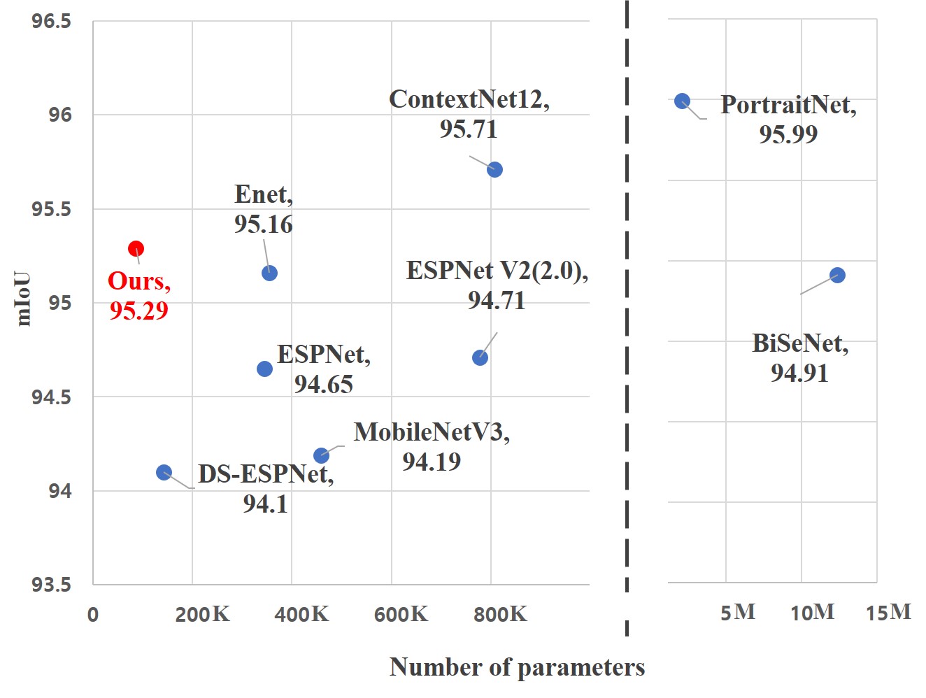
Figure 1: Accuracy (mIoU) vs. complexity (number of parameters) on the EG1800 validation set. Our proposed SINet has high accuracy with small complexity.

1 Introduction

Developing algorithms targeting face data has been considered as an important task in the computer vision field, and many related vision algorithms including detection, recognition, and key-point extraction are actively studied. Among them, portrait segmentation is commonly used in real-world applications such as background editing, security checks, and face resolution enhancement [19, 29], giving rise to the need for fast and robust segmentation models.

The challenging point of the segmentation task is that the model have to solve two contradictory problems simultaneously; (1) Handling long-range dependencies or global consistency and (2) preserving detailed local information. Figure 2 shows two common segmentation errors. First, the blue blob in Figure 2 (b) is classified as foreground, even though it is easily recognized as a wood region. The reason for this problem is that the segmentation model fails to get global context information which prevents wrong representation. Second, the red blobs in Figure 2 (b) show the model’s failure to accurately segment fine details. The lateral part of hair needs fine segmentation due to its small size and similar color to the wood. The model is not able to produce a sharp segmentation image because of the lack of detail information about hair. This is because the usage of stride convolution or pooling layer. These techniques induces the model can capture global information by enlarging receptive field size. However, the local information might be destroyed.

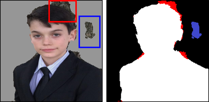
(a) Input image	(b) Typical segmentation errors
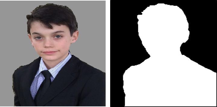
(c) Ground truth	(d) Example of Ours

Figure 2: Typical examples of segmentation errors. (b) The wood region is failed to be suppressed and the boundary of the boy’s hair is not sharply segmented. (d) Our method solves the problem without heavy computation.

Researchers have developed several strategies to solve these problems and the first one is to produce multiple receptive fields for each layer. This multi-path structure is able to enhance both global and local information, but comes at the cost of increased latency due to fragmented parallel operations [10]. Another method is using a two-branch network, which consists of a deeper branch that is employed to produce global context, and a shallow branch that preserves detailed local features by keeping high resolution [16, 17, 27]. Even though the shallow branch has few convolutional layers, it is computationally heavy due to its high-resolution feature maps. Also, this method has to extract features two times, once for each branch.

The portrait segmentation problem comes with a set of additional challenges. The first one being the small amount of available data. The EG1800 dataset [19], an accessible public portrait segmentation dataset, contains only around 1,300 training images, and has large biases with regard to attributes such as race, age, and gender. Second, portrait segmentation is usually used just as one of several steps in real-world applications. Since many of these applications run on mobile devices, the segmentation model needs to be lightweight to ensure real-time speeds. Researchers have developed plenty of lightweight segmentation methods, but most of them are still not lightweight enough for portrait segmentation tasks. For example, PortraitNet [29], the current state-of-the-art model on the EG1800 dataset, has $2.1M$ parameters. A few examples of general lightweight segmentation models are ESPNetV2 [11] with $0.78M$ parameters, and MobileNet V3 [6] with $0.47M$ parameters.

In this paper, we propose a new extremely lightweight portrait segmentation model called SINet with an information blocking decoder structure and spatial squeeze modules (S2-module). Furthermore, we collect additional portrait segmentation data to overcome the aforementioned dataset problems. The proposed SINet has 86.9K parameters, achieving 100.6 FPS in iPhone XS without any low-floating point operations or pruning methods. Compared with the baseline model, PortraitNet, which has 2.1M parameters, the accuracy degradation is just under $1\%$ on the EG1800 dataset, as can be seen in Figure 1.

Our contributions can be summarized as follows: (1) We introduce the information blocking scheme to the decoder. It measures the confidence in a low-resolution feature map, and blocks the influence of high-resolution feature maps in highly confident pixels. This prevents noisy information to ruin already certain areas, and allows the model to focus on regions with high uncertainty. We show that this information blocking decoder is robust to translation and can be applied to general segmentation tasks. (2) We propose a spatial squeeze module (S2-module), an efficient multi-path network for feature extraction. Existing multi-path structures deal with the various size of long-range dependencies by managing multiple receptive fields. However, this increases latency in real implementations, due to having unsuitable structure with regard to kernel launching and synchronization. To mitigate this problem, we squeeze the spatial resolution from each feature map by average pooling, and show that this is more effective than adopting multi-receptive fields. (3) The public portrait segmentation dataset has a small number of images compared to other segmentation datasets, and is highly biased. We propose a simple and effective data generation method to augment the EG1800 dataset with a significant amount of images.

2 Related Work

Portrait Application: PortraitFCN+ [19] built a portrait dataset from Flickr and proposed a portrait segmentation model based on FCN [9]. After that, PortraitNet proposed a real-time portrait segmentation model with higher accuracy than PortraitFCN+. [13] integrated two different segmentation schemes from Mask R-CNN and DensePose, and generated matting refinement based on FCN. [5] introduced a boundary-sensitive kernel to enhance semantic boundary shape information. While these works achieved good segmentation results, their models are still too heavy for embedded systems.

Global consistency: Global consistency and long range of dependencies are critical factors for the segmentation task, and models without a large enough receptive field will produce error-prone segmentation maps. One way of creating a large receptive field is to use large kernels. However, this is not suitable for lightweight models due to their large number of parameters. Another method is to reduce the size of feature maps through downsampling, but this leads to difficulties in segmenting small or narrow objects.

To resolve this problem, dilated convolutions (or atrous convolutions) have been introduced as an effective solution to get a large receptive field while preserving localization information [28, 2], keeping the same amount of computation as the normal convolution. However, as the dilation rate is increased the count of valid weights decreases, to finally degenerate to a $1\times 1$ convolution  [3]. Also, the grid effect degrades the segmentation result with checker-board pattern. Another method is to use spatial pyramid pooling to get a larger receptive field. The spatial pyramid pooling uses different sizes of pooling and concatenates each resultant feature map to obtain a multi-scale receptive field. Similarly, the Atrous Spatial Pyramid Pooling layer [4] replaces the pooling with dilated convolutions to get a multi-scale representation. To get a multi-scale representation, some works use a multi-path structure for feature extraction [18, 11, 14]. Each module splits the input feature map and translates the feature map with a different dilation rate. This method is well suited for lightweight models, but suffers from high latency. Recently, the asymmetric non-local block [30] was proposed, inspired by the non-local block [23] and spatial pyramid pooing. Because the non-local block calculates all the pairwise pixel dependencies, it is computationally heavy. Asymmetric non-local block approximates the calculation with spatial pyramid pooling. However, the computational cost is still too large to fit a lightweight model.Recently, some works adopt average pooling to reduce complexity more [21, 7].

Detail local information: Recovering detailed local information is crucial to generating sharp segmentation maps. Conventionally, an encoder-decoder structure based on deconvolution (or transposed convolution) is applied [9, 12]. By concatenating the high-resolution feature, they recover the original resolution step by step. Also, some works use global attention for upsampling. The feature pyramid attention [8] uses global pooling to enhance the high resolution feature map from the low-resolution. However, the attention vector can not reflect the local information well due to global pooling. Recently, the two-branch method is suggested for better segmentation. ContextNet [16] and FastSCNN [17] designed a two-path network, each branch of which is for global context and detailed information, respectively. BiSeNet [27] also proposed a similar two-path network for preserving spatial information as well as acquiring a large enough receptive field. However, it needs to calculate features twice, once for each branch.

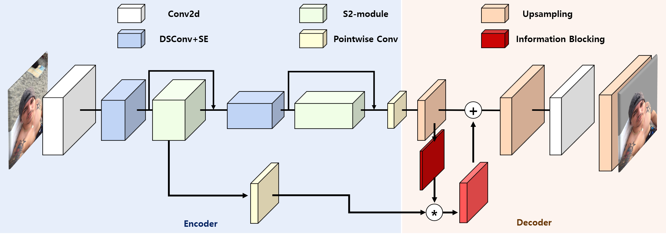
(a)

Figure 3: The overall architecture of SINet. The S2-module is the bottleneck in SINet and the information blocking decoder makes fine segmentation results. DSConv+SE means depthwise separable convolution with a Squeeze-and-Excitation block

3 Method

In this section, we explain the structure of the proposed SINet which consists of a Spatial squeeze module and a Information blocking decoder. The spatial squeeze block (S2-module) handles global consistency by using the multi-receptive field scheme, and squeezes the feature resolution to mitigate the high latency of multi-path structures. The information blocking decoder is designed to only take the necessary information from the high-resolution feature maps by utilizing the confidence score of the low-resolution feature maps. The information blocking in the decoder is important for increasing robustness regarding translation (Section 3.1) and the S2-module can handle global consistency without heavy computation (Section 3.2). We also demonstrate a simple data generation framework to solve the lack of data in two situations: 1) having human segmentation ground truths and 2) having only raw images (Section 3.4).

3.1 Information Blocking Decoder

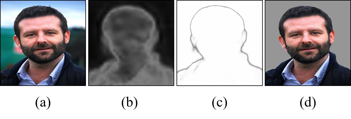
Figure 4: From left to right,(a) an input image, (b) an information blocking map, (c) a confidence map of last block in model and (d) the segmentation results from the proposed method. The information blocking map helps to prevent inflow of nuisance features, and makes the model focus more on regions with high uncertainty.

An encoder-decoder structure is the most commonly used structure for segmentation. An encoder extracts semantic features of the incoming images according to semantic information, and a decoder recovers detailed local information and resolution of the feature map. For designing the decoder, bilinear upsampling or transposed convolution upsampling blocks are commonly used to expand the low-resolution feature maps from the encoder. Also, recent works [18, 14, 6, 4] re-use additional high-resolution feature maps from the encoder to make more accurate segmentation results. To the best of our knowledge, most studies take all the information of high-resolution feature maps from the encoder by conducting concatenation, element-wise summation, or by enhancing high-resolution feature maps via attention vectors from low-resolution. However, using the high-resolution feature maps means that we give nuisance local information, which is already removed by the encoder. Therefore, we have to take only the necessary clue and avert the nuisance noise.

Here, we introduce a new concept of a decoder structure using information blocking. We measure the confidence score in the low-resolution feature map and block the information flow from the high-resolution feature into the region where the encoder successfully segmented with high confidence. The information blocking process removes nuisance information from the image and makes the high-resolution feature map concentrate only on the low confidence regions.

Figure 3 shows the overall architecture of SINet and the detailed process of the information blocking decoder. The model projects the last set of feature maps of the encoder to the size of the number of classes by a pointwise convolution and uses a bilinear upsampling to make the same resolution as the high-resolution target segmentation map. The model employs a softmax function to get a probability of each class and calculates each pixel’s confidence score $c$ by taking maximum value among the probabilities of each class. Finally, we generate an information blocking map by computing $(1-c)$. We perform pointwise multiplication between the information blocking map and the high-resolution feature maps. This ensures that low confidence regions get more information from the high-resolution feature maps, while high confidence regions keep their original values in the subsequent pointwise addition operation.

Figure 4 (b) is an example of the information blocking map, and (c) is the confidence map from the model output. As shown in Figure 4 (b), the boundary and clothing have high uncertainty while the inner parts of the foreground and background already have a high confidence score. This indicates that the high uncertainty regions need more detailed local information to reduce uncertainty. However, the inner parts of the face, such as the beard and nose, do not need to get more local information for making a segmentation map. If the local information was embedded, it could be harmful to the global consistency due to nuisance information as noise. In the final confidence map of the model (Figure. 4 (c)), the uncertainty region of the boundary has shrunk, and the confidence score of the inner part is highly improved.

3.2 Spatial Squeeze module

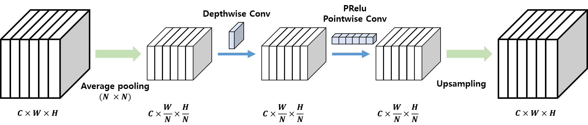
(a) Spatial Squeeze Block (S2-block).

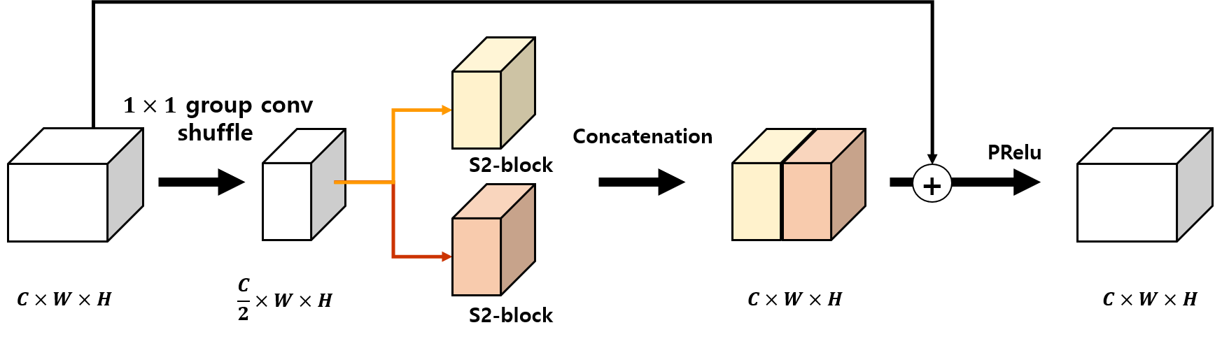
(b) Spatial Squeeze Module (S2-module).

Figure 5: (a) An input feature map is squeezed by an $N\times N$ average pooling before a depthwise convolution. Then, a bilinear upsampling recovers the original input resolution of the feature maps. (b) The S2-module has multi-receptive structures by using different combinations of convolution kernels and pooling for the S2-blocks.

Dilated rate	rate=2	rate=6	rate=12	rate=18
Latency (ms)	6.7	6.63	11.84	12.03

Table 1: Latency running depthwise separable dilated convolution with different dilation rates on an iPhone XS. The input size is $128\times 120\times 120$. Additional experiments with other input sizes are reported in the supplementary material.

A multi-path structure have an advantage of high accuracy with less parameters [21, 20, 20, 25], but it suffers from increased latency proportional to the number of sub-paths [10]. The proposed spatial squeeze module (S2-module) resolves this problem and Figure 5 shows the structure. We utilize average pooling for adjusting the size of the receptive field and reducing the latency.

The S2-module is also following a kind of split-transform-merge scheme like [18, 11, 14] for covering multi-receptive field with two spatial squeeze blocks (S2-block). First, we uses a pointwise convolution to reduce the number of feature maps by half. For further reduction of computation, we use a group pointwise convolution with channel shuffle. The reduced feature maps pass through each S2-block, and the results are merged through concatenation.We also adopt a residual connection between the input feature map and the merged feature map. Finally, PRelu is utilized for non-linearity.

For S2-block, we select average pooling rather than dilated convolution for making a multi-receptive field structure for two reasons. First, the latency time is affected from the dilated rate, as shown in Table 1, and dilated convolution can not be free from the problem of grid effects [14, 22]. Second, the multi-path structure is not friendly to GPU parallel computing [10]. Thus, we squeeze the resolution of each feature map to avoid the sacrifice of the latency time. The S2-block squeezes the resolution of a feature map by an average pooling, with kernel size up to 4. Then, a depthwise separable convolution with the kernel size $3$ or $5$ is used. Between the depthwise convolution and the pointwise convolution, we use a PRelu non-linear activation function. Empirically, placing the pointwise convolution before or after the bilinear upsampling does not have a critical effect on the accuracy. Therefore, we put it before the bilinear upsampling to further reduce computation. We also insert a batch normalization layer after the depthwise convolution and the bilinear upsampling.

3.3 Network Design for SINet

	Input	Operation	Output
1	$3\times 224\times 224$	CBR	$12\times 112\times 112$	Down sampling
2	$12\times 112\times 112$	DSConv+SE	$16\times 56\times 56$	Down sampling
3	$16\times 56\times 56$	SB module	$48\times 56\times 56$	[k=3, p=1], [k=5, p=1]
4	$48\times 56\times 56$	SB module	$48\times 56\times 56$	[k=3, p=1], [k=3, p=1]
5	$64\times 56\times 56$	DSConv+SE	$48\times 28\times 28$	Concat [2, 4], Down sampling
6	$48\times 28\times 28$	SB module	$96\times 28\times 28$	[k=3, p=1], [k=5, p=1]
7	$96\times 28\times 28$	SB module	$96\times 28\times 28$	[k=3, p=1], [k=3, p=1]
8	$96\times 28\times 28$	SB module	$96\times 28\times 28$	[k=5, p=1], [k=3, p=2]
9	$96\times 28\times 28$	SB module	$96\times 28\times 28$	[k=5, p=2], [k=3, p=4]
10	$96\times 28\times 28$	SB module	$96\times 28\times 28$	[k=3, p=1], [k=3, p=1]
11	$96\times 28\times 28$	SB module	$96\times 28\times 28$	[k=5, p=1], [k=5, p=1]
12	$96\times 28\times 28$	SB module	$96\times 28\times 28$	[k=3, p=2], [k=3, p=4]
13	$96\times 28\times 28$	SB module	$96\times 28\times 28$	[k=3, p=1], [k=5, p=2]
14	$144\times 28\times 28$	1x1 conv	$\#class\times 28\times 28$	Concat [5, 13]

Table 2: Detailed settings for the SINet encoder. k denotes the kernel size of the depthwise convolution and p denotes the kernel size of average pooling the S2-block.

In this part, we explain the overall structure of SINet. SINet uses S2-modules as bottlenecks and depthwise separable convolution (ds-conv) with stride $2$ for reducing the resolution of feature maps. Empirically, applying the S2-module with stride $2$ for downsampling improves accuracy, but we found that it has longer latency time than S2-module with stride $1$ under the same output size conditions. Therefore, for downsampling, instead of the S2-module with stride 2, we use ds-conv with Squeeze-and-Excite blocks. For the first bottleneck we use two sequential S2-modules and for the second bottleneck we use eight. The detailed setting of the S2-module is described in Table 2. We add a residual connection for each bottleneck, concatenating the bottleneck input with its output. A $3\times 3$ convolution is used for classification and finally bilinear upsampling is applied to recover the original input resolution.

We found that a weighted auxiliary loss for the boundary part is helpful in improving the accuracy. The final loss is as follows:

$$\mathcal{B}=(f\oplus y^{*})-(f\ominus y^{*})$$ (1)

$$Loss=CE_{i\in\mathcal{P}}(y_{i}^{*},\hat{y})+\lambda CE_{j\in\mathcal{B}}(y_{j}^{*},\hat{y}_{j}).$$

Here, $f$ is a $15\times 15$ filter used for the morphological dilation ($\oplus$) and erosion ($\ominus$) operations. $\mathcal{P}$ denotes all the pixels of the ground truth, and $\mathcal{B}$ denotes the pixels in the boundary area as defined by the morphology operation. $y^{*}$ is a binary ground truth value and $\hat{y}$ is a predicted label from a segmentation model. $\lambda$ is a hyperparameter that controls the balance between the loss terms.

Method	Parameters (M)	FPS	FLOPs (G)	F1-score	mIOU	mIOU [29]
Enet (2016) [15]	0.355	8.06	0.346	0.917	95.16	96
BiSeNet (2018) [27]	0.124	2.99	2.31	0.908	94.91	95.25
PortraitNet (2019)[29]	2.08	3.30	0.325	0.919	95.99	96.62
ESPNet (2018)[18]	0.345	6.99	0.328	0.883	94.65	-
DS-ESPNet	0.143	7.75	0.199	0.866	94.10	-
DS-ESPNet(0.5)	0.064	9.26	0.139	0.859	93.58	-
ESPNetV2(2.0) (2019)[11]	0.778	3.65	0.231	0.872	94.71	-
ESPNetV2(1.5) (2019)[11]	0.458	4.95	0.137	0.861	94.00	-
ContextNet12 (2018)[16]	0.838	1.55	1.87	0.896	95.71	-
MobileNetV3 (2019)[6]	0.458	10.87	0.066	0.854	94.19	-
SINet(Ours)	0.087	12.35	0.064	0.884	94.81	-
SINet+(Ours)	0.087	12.35	0.064	0.892	95.29	-

Table 3: EG1800 validation results for the proposed SINet and other segmentation models. DS denotes depth-wise separable convolution. We measure FPS on an Intel Core 15-7200 CPU environment with input size $224\times 224$. The results in the last column are from the PortraitNet [29] paper. SINet+ is the result of using the augmented dataset as descibed in Section 3.4

3.4 Data Generation

Annotating data often comes with high costs, and the annotation time per instance varies a lot depending on the task type. For example, the annotation time per instance for PASCAL VOC is estimated to be 20.0 seconds for image classification and 239.7 seconds for segmentation, an order of magnitude difference as mentioned in [1] . To mitigate the cost of annotation for portrait segmentation, we consider a couple of plausible situations: 1) having images with ground truth human segmentation. 2) having only raw images. We make use of either an elaborate face detector model (case 1) or a segmentation model (case 2) for generating pseudo ground truths to each situation.

When we have human images and ground truths, the only thing we need is a bounding box around the portrait area. We took images from Baidu dataset [24], which contains 5,382 human full body segmentation images covering various poses, fashions and backgrounds. To get the bounding box and portrait area, we detect the face location of the images using a face detector [26]. Since the face detector tightly bounds the face region, we increase the bounding box size to include parts of the upper body and background before cropping the image and ground truth segmentation.

We also create a second augmentation from portrait images scraped from the web, applying a more heavyweight segmentation model to generate pseudo ground truth segmentation masks. This segmentation model consists of a DeepLabv3+ [4] architecture with a SE-ResNeXt-50 [25] backbone. The model is pre-trained on ImageNet and finetuned on a proprietary dataset containing around 2,500 fine grained human segmentation images. The model is trained for general human segmentation rather than for the specific purpose of portrait segmentation.

Finally, human annotators just check the quality of each pseudo ground truth image, removing obvious failure cases. This method reduces the annotation effort per instance from several minutes to 1.25 seconds by transforming the segmentation task into a binary classification task.

4 Experiment

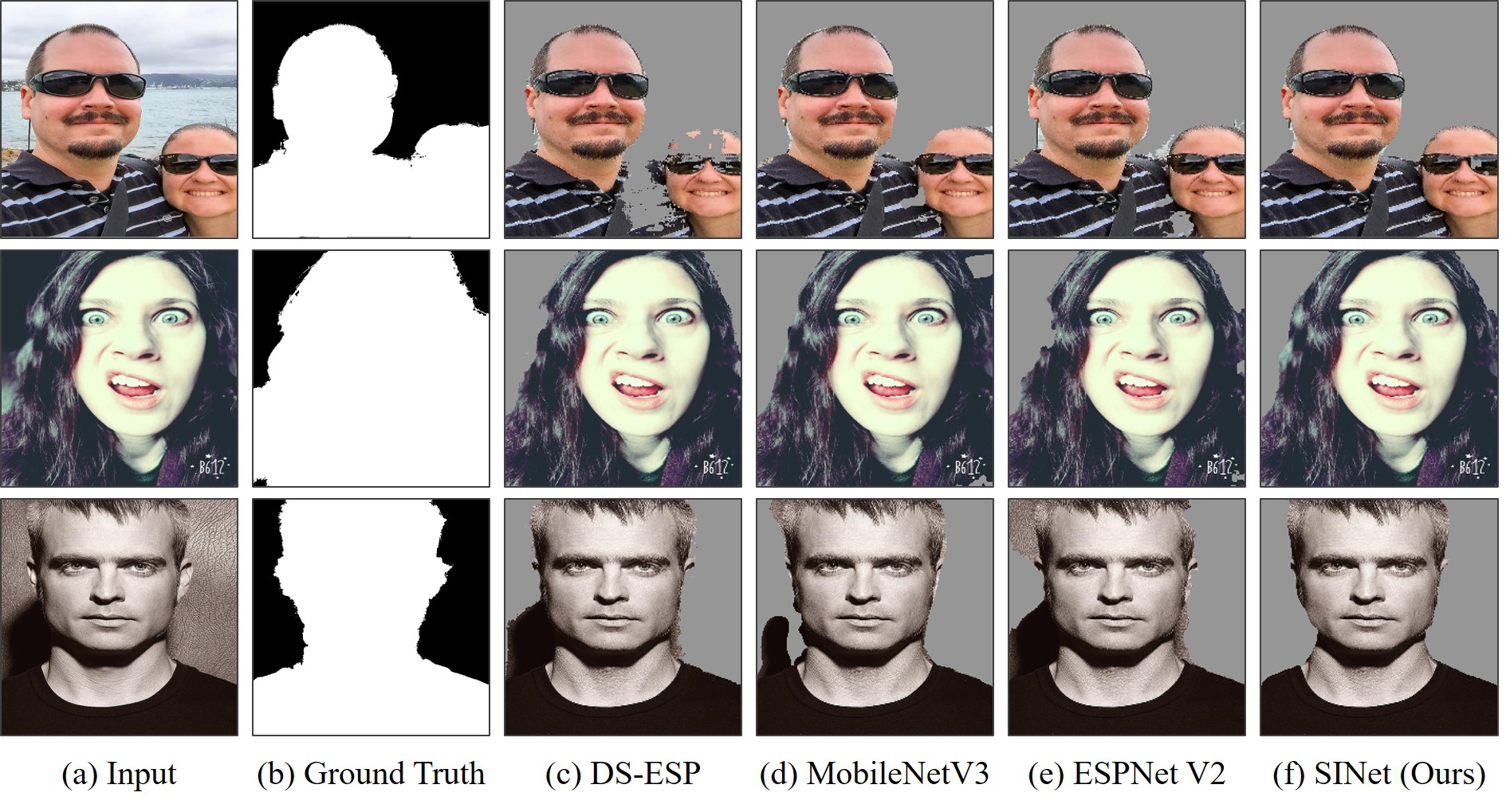
Figure 6: Qualitative comparison results on the EG1800 validation dataset.

We evaluated the proposed method on the public dataset EG1800 [19], which collected images from Flickr with manually annotated labels. The dataset has a total of $1,800$ images and is divided into $1,500$ train and $300$ validation images. However, we could access only 1,309 images for train and 270 for validation, since some of the URLs are broken. We built an additional 10,448 images using the proposed data generation method mentioned in Section  3.4.

We trained our model using ADAM optimizer with initial learning rate to $7.5\mathrm{e}{-3}$, and weight decay to $2\mathrm{e}{-4}$, for a total of 600 epochs. We followed the data augmentation method in [29] with $224\times 224$ images. We used a two-stage training method;for the first 300 epochs, we only trained until the encoder with the batch size set to $36$. Then, we initialize the encoder with the best parameters from the previous step, and trained the overall SINet model for an additional 300 epochs with the batch size to $24$. We evaluated our model followed by various ablations using mean intersection over union (mIoU) and F1-score in the boundary part, and compared with SOTA portrait segmentation models including other lightweight segmentation models. To define the boundary region, we subtract the eroded ground truths from the dilated ground truths, using a kernel with size $15\times 15$. We demonstrated the robustness of the information blocking decoder on randomly rotated EG1800 validation images, and the importance of multi-receptive structure on EG1800 validation images in Section 4.2 Also, we showed that the proposed method can be used for general tasks by evaluating it on the Cityscapes dataset.

4.1 Evaluation Results on the EG1800 Dataset

We compared the proposed model to PortraitNet[29], which has SOTA accuracy in the portrait segmentation field. Since some sample URLs in the EG1800 dataset are missing, we re-trained the PortraitNet following the original method in paper and using the official code on the remaining samples in EG1800 dataset. PortraitNet compared their work to BiseNet and Enet. Therefore, we also re-trained BiSeNet and ENet following the method of PortraitNet for a fair comparison. As shown in Table 3, the accuracies of the re-trained models are slightly decreased due to the reduced size of the training dataset. We measured latency time on an Intel Core i5-7200U CPU environment with the PyTorch framework on an LG gram laptop.

Among the compared methods, DS-ESPNet has the same structure as ESPNet, with only changing the standard dilated convolutions of the model into depth-wise separable dilated convolutions. For ESPNetV2 (2.0) and ESPNetV2 (1.5), we changed the number of channels of the convolutional layers to reduce the model size as following official code. We also reduced the number of channels for the convolutions in the DS-ESPNet (0.5) by half from the original model to make it less than 0.1M parameters and 0.2G FLOPs. The original ContextNet used 4 pyramid poolings but we used only 3 due to the small feature map size.

From Table 3, we see that our proposed method achieved comparable or better performance than the other models, while having less parameters and FLOPs, and higher FPS. The SOTA PortraitNet showed the highest accuracy in all the experimental results, and has achieved even better performance than the heavier BiSeNet. However, PortraitNet requires a large number of parameters, which is a disadvantage for using it on smaller devices. The proposed SINet has reduced the number of parameters by 95%, and FLOPs by 80% compared to PortraitNet, while maintaining accuracy. ESPNet and ESPNet V2 have similar accuracy, but showed a trade-off between the number of parameters and FLOPs. ESPNet V2 has more parameters than ESPNet, but ESPNet needs more FLOPs than ESPNet V2. Enet shows better performance than both models but requires more FLOPs. In our comparison, the proposed method has less number of parameters and FLOPs, but still achieved better accuracy than ESPNet and ESPNet V2. In particular, our SINet has the highest accuracy in an extremely lightweight environment. Figure 6 shows that the quality of our model is superior to other extremely lightweight models.

We compared the execution speed of the proposed model with SOTA segmentation model MobileNet V3 on an iPhone XS using the CoreML framework. MobileNet V3 has 60.7 FPS, and our SINet has 100.6 FPS. The FLOPs in MobileNet V3 and SINet are similar, but SINet is much faster than MobileNet V3. We conjecture that the SE block and h-swish activation function are the main reasons for the increase in latency in MobileNet V3. In summary, the proposed SINet showed outstanding performance among the various segmentation model in terms of accuracy and speed.

4.2 Ablation Study

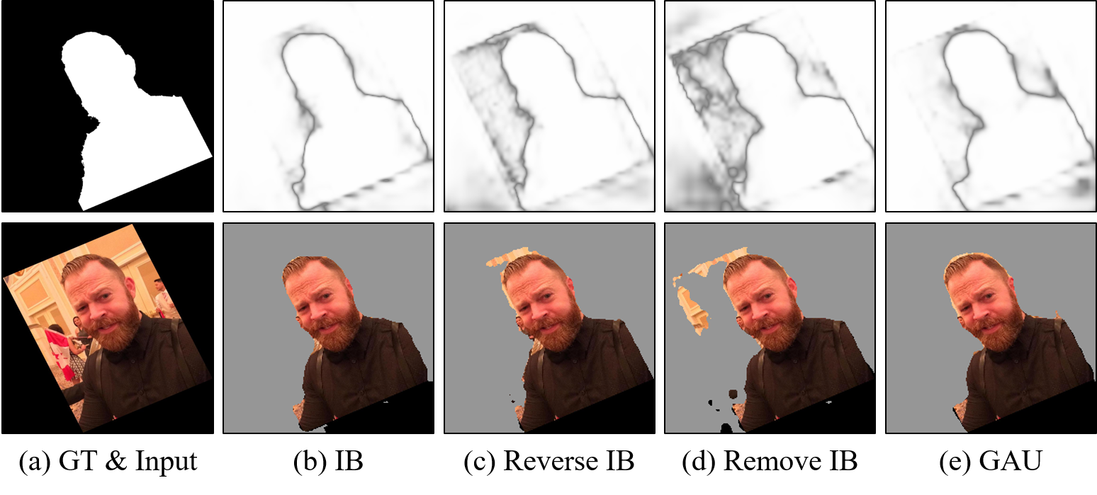
Figure 7: Confidence maps of the last features from the model and segmentation results according to the decoding method.

	Org	$25^{\circ}$	$45^{\circ}$	$75^{\circ}$	$90^{\circ}$
IB	94.81	88.62	84.74	79.05	76.85
Reverse IB	94.68	84.06	80.58	73.88	73.09
Remove IB	94.74	85.11	81.53	75.36	72.99
GAU [8]	94.77	86.33	82.80	75.85	73.96

Table 4: mIOU results when using random rotations ($-x^{\circ}\sim x^{\circ}$). Org denotes original validation image without any translation. IB denotes using information blocking map and Reverse IB enhances high-confidence regions rather than low-confidence ones.

Information blocking decoder: Table 4 shows the accuracy improvement from using the information blocking decoder. We randomly rotated validation images and evaluated mIOU over the whole image. Reverse IB denotes that we multiply the high-resolution feature maps with the confidence score $c$ instead of $(1-c)$, thus enhancing high-confident pixels rather than low-confidence ones. Remove IB means that we did not use any information blocking, and instead conducted element-wise summation between the low-resolution feature maps and the high-resolution feature maps from a middle layer of a encoder. GAU uses global pooling to enhance high-resolution feature map from low-resolution feature map before applying element-wise summation. GAU has better performance than Reverse IB and Remove IB, but it still fails to get a tight boundary and to get better performances in translated images than IB. From the result, we can see that the information blocking decoder shows outstanding performance compared to the other methods. Qualitatively, it prevents segmentation errors of the background region as shown in Figure 7.

Multi-receptive field:

Convolution	Pooling	mIOU	f1-score
3	1	93.40	0.874
3	2	93.34	0.851
3	4	90.34	0.796
5	1	94.56	0.881
5	2	93.11	0.857
5	4	90.04	0.799
SINet (Ours)		94.81	0.884

Table 5: Ablation study for the S2-module. Our multi-receptive structure achieved better accuracy than the other settings.

Table 5 shows the performance depending on the multi-receptive structures. SINet used various combinations of kernel sizes for convolution and pooling. We re-designed the S2-module to always use the same kernel sizes within the S2-block for all convolutional and pooling layers respectively. As shown in Table 5, our SINet achieved higher mIOU and F1-score than the other combinations. Therefore, a multi-receptive field structure has an advantage for accuracy than a single-receptive field one.

4.3 General Segmentation Dataset

	Param(M)	FLOP(f)	FLOP(h)	mIOU
ESPNet	0.36	-	4.5	61.4
ContextNet14	0.85	5.63	-	66.1
ESPNetV2	0.79	-	2.7	66.2
MobileNetV2(0.35)	0.16	2.54	-	66.83(val)
MobileNetV3-small	0.47	2.9	-	69.4
SINet (Ours)	0.12	1.2	-	66.5

Table 6: Semantic segmentation results on the Cityscapes test set. FLOP(f) means that the number of FLOPs was measured with full-resolution input, $2048\times 1024$. FLOP(h) denotes that the number of FLOPs was measured with half-resolution, $1024\times 512$.

	Input	Operation	Output
1	$3\times 1024\times 2048$	CBR	$16\times 512\times 1024$	Down sampling
2	$16\times 512\times 1024$	DSConv + SE	$\#class\times 256\times 512$	Down sampling
3	$\#class\times 256\times 512$	DSConv + SE	$24\times 128\times 256$	Down sampling
4	$24\times 128\times 256$	SB module	$60\times 128\times 256$	[k=3, p=1], [k=5, p=1]
5	$60\times 128\times 256$	SB module	$60\times 128\times 256$	[k=3, p=0], [k=3, p=1]
6	$60\times 128\times 256$	SB module	$60\times 128\times 256$	[k=3, p=0], [k=3, p=1]
7	$84\times 128\times 256$	DSConv + SE	$60\times 64\times 128$	Concat [3, 6] , Down sampling
8	$60\times 64\times 128$	SB module	$84\times 64\times 128$	[k=3, p=1], [k=5, p=1]
9	$84\times 64\times 128$	SB module	$84\times 64\times 128$	[k=3, p=0], [k=3, p=1]
10	$84\times 64\times 128$	SB module	$84\times 64\times 128$	[k=5, p=1], [k=5, p=4]
11	$84\times 64\times 128$	SB module	$84\times 64\times 128$	[k=3, p=2], [k=5, p=8]
12	$84\times 64\times 128$	SB module	$108\times 64\times 128$	[k=3, p=1], [k=5, p=1]
13	$108\times 64\times 128$	SB module	$108\times 64\times 128$	[k=3, p=1], [k=5, p=1]
14	$108\times 64\times 128$	SB module	$108\times 64\times 128$	[k=3, p=0], [k=3, p=1]
15	$108\times 64\times 128$	SB module	$108\times 64\times 128$	[k=5, p=1], [k=5, p=8]
16	$108\times 64\times 128$	SB module	$108\times 64\times 128$	[k=3, p=2], [k=5, p=4]
17	$108\times 64\times 128$	SB module	$108\times 64\times 128$	[k=3, p=0], [k=5, p=2]
18	$168\times 64\times 128$	1x1 conv	$\#class\times 64\times 128$	Concat [7, 17]

Table 7: Detailed settings for the SINet encoder. k denotes the kernel size of the depthwise convolution and p denotes the kernel size of average pooling the S2-block.

We also demonstrate that our proposed method is suitable not only for the binary segmentation problem but also for general segmentation problems by testing the model on the Cityscapes dataset. We increased the number of layers and channels a little bit to cope with the increased complexity compared to the binary segmentation task, and we factorized the depthwise convolution in the S2-blocks for reducing the number of parameters. Here, SINet has only 0.12M parameters and 1.2GFLOPs for input of size $2048\times 512$, but our model showed better accuracy than any other lightweight segmentaiton model except MobileNet V3 and MobileNet V2. The accuracy of SINet decreases by 2.9% with respect to MobileNet V3, but the number of parameters and FLOPs are much lower than MobileNet V3. Table 7 is a detailed setting of the encoder model for the Cityscape segmentation.

5 Conclusion

In this paper, we proposed an extremely lightweight portrait segmentation model, SINet, which consists of an information blocking decoder and spatial squeeze modules. SINet executes well in mobile device with 100.6FPS and has high accuracy with 95.29. The information blocking decoder prevents nuisance information from high-resolution features and induce the model to concentrate more on high uncertainty regions. The spatial squeeze module has multi-receptive field to handle the various sizes of global consistency in an image. We also proposed a simple data generation framework covering the two situations: 1) having human segmentation ground truths 2) having only raw images. Not only on the specific portrait dataset but also on the general segmentation dataset, our model obtained outstanding performance compared to the existing lightweight segmentation models from the experiments. The proposed method shows appropriate accuracy (66.5 %) with only 0.12M number of parameter and 1.2G FLOP on the Cityscapes dataset.

Appendix

Additional Experiment Results

Input Resolution	$48\times 48$
Input Channel	32				128
	Min	Mean	Max	Total	Min	Mean	Max	Total
$d=2$	1.4	1.6	1.99	159.91	1.64	1.92	2.75	192.29
$d=6$	1.41	1.66	1.98	166.08	1.67	1.92	2.69	192.75
$d=12$	2.63	5.22	9.16	524.23	4.32	8.63	11.78	866.7
$d=18$	3.05	5.42	9.96	544.49	3.52	8.38	12.04	841.26
Input Resolution	$120\times 120$
Input Channel	32				128
	Min	Mean	Max	Total	Min	Mean	Max	Total
$d=2$	5.22	5.54	8.44	555.17	6.36	6.7	11.21	671.03
$d=6$	4.86	5.36	7.79	536.96	6.42	6.63	11	663.61
$d=12$	8.99	14.03	25.65	1403.78	9.2	11.84	15.18	1184.8
$d=18$	9.09	13.84	24.51	1384.74	9.48	12.03	15.45	1204.13
Input Resolution	$320\times 320$
Input Channel	32				128
	Min	Mean	Max	Total	Min	Mean	Max	Total
$d=2$	26.92	27.76	49.53	2777.01	36.33	37.23	73.88	3724.02
$d=6$	27.02	28.13	48.41	2813.39	36.25	37.48	73.78	3748.36
$d=12$	30.7	31.84	52.32	3184.4	46.31	47.74	78.9	4774.73
$d=18$	31.45	32.66	55.9	3267.09	46.54	47.84	79.86	4785.13

Table 8: Latency time experiments about depthwise separable dilated convolution on iPhone CPU/GPU/NPU environment. All performance value are reported in milliseconds. d denotes a dilated rate of convolution filter.

	CPU
Model	Min	Mean	Max	Total
SINet	9.69	9.8	12.1	980.11
MobileNet V3	15.81	16.07	19.2	1607.54
ESPNet V2	95.79	96.48	103.44	9649.16
	CPU/GPU
Model	Min	Mean	Max	Total
SINet	44.51	83.01	123.84	8303.74
MobileNet V3	48.9	110.53	145.87	11056.51
ESPNet V2	59.83	91.53	640	9154.22
	CPU/GPU/NPU
Model	Min	Mean	Max	Total
SINet	9.63	9.94	16.94	994.45
MobileNet V3	15.88	16.18	26.28	1619.12
ESPNet V2	36.87	37.65	46.6	3766.04

Table 9: Latency time experiments under different environments. We converted ESPNet V2 Pascal VOC segmentation model by CoreML framework from their official converting code for baseline of latency time in a mobile environment. The input size of SINet and MobileNet V3 is $224\times 224$ and the input size of ESPNet V2 is $256\times 256$. The number of FLOPs of SINet, MobileNet V3 and ESPNet V2 are $0.064G$, $0.066$ and $0.338G$. Our SINet is faster than MobileNet V3 and ESPNet V2 in all the environments. All performance value are reported in milliseconds

The goal of this experiment is to show exact performances on different types of layers or models that run on iOS. We are running on all the experiments with iPhone XS Max and iOS 13.1.2. We did 100 iterations and waited 2 seconds between each run, and all performance values are reported in milliseconds. Each model in Table 8 are tested on CPU/GPU/NPU configuration and each model in Table 9 are executed in different configuration (CPU, CPU/GPU, CPU/GPU/NPU ). As shown in Table 8, a large dilated rate convolution layer is slower than others regardless of input size. Table 9 proves that our SINet is faster than any other model in every configuration. This result demonstrates that our model can be applied to any configurations well.

References

- [1] A. Bearman, O. Russakovsky, V. Ferrari, and L. Fei-Fei. What’s the point: Semantic segmentation with point supervision. In European conference on computer vision, pages 549–565. Springer, 2016.
- [2] L.-C. Chen, G. Papandreou, I. Kokkinos, K. Murphy, and A. L. Yuille. Deeplab: Semantic image segmentation with deep convolutional nets, atrous convolution, and fully connected crfs. IEEE transactions on pattern analysis and machine intelligence, 40(4):834–848, 2018.
- [3] L.-C. Chen, G. Papandreou, F. Schroff, and H. Adam. Rethinking atrous convolution for semantic image segmentation. arXiv preprint arXiv:1706.05587, 2017.
- [4] L.-C. Chen, Y. Zhu, G. Papandreou, F. Schroff, and H. Adam. Encoder-decoder with atrous separable convolution for semantic image segmentation. In ECCV, 2018.
- [5] X. Du, X. Wang, D. Li, J. Zhu, S. Tasci, C. Upright, S. Walsh, and L. Davis. Boundary-sensitive network for portrait segmentation. In 2019 14th IEEE International Conference on Automatic Face & Gesture Recognition (FG 2019), pages 1–8. IEEE, 2019.
- [6] A. Howard, M. Sandler, G. Chu, L.-C. Chen, B. Chen, M. Tan, W. Wang, Y. Zhu, R. Pang, V. Vasudevan, et al. Searching for mobilenetv3. arXiv preprint arXiv:1905.02244, 2019.
- [7] D. Li, A. Zhou, and A. Yao. Hbonet: Harmonious bottleneck on two orthogonal dimensions. arXiv preprint arXiv:1908.03888, 2019.
- [8] H. Li, P. Xiong, J. An, and L. Wang. Pyramid attention network for semantic segmentation. arXiv preprint arXiv:1805.10180, 2018.
- [9] J. Long, E. Shelhamer, and T. Darrell. Fully convolutional networks for semantic segmentation. In Proceedings of the IEEE conference on computer vision and pattern recognition, pages 3431–3440, 2015.
- [10] N. Ma, X. Zhang, H.-T. Zheng, and J. Sun. Shufflenet v2: Practical guidelines for efficient cnn architecture design. In Proceedings of the European Conference on Computer Vision (ECCV), pages 116–131, 2018.
- [11] S. Mehta, M. Rastegari, L. Shapiro, and H. Hajishirzi. Espnetv2: A light-weight, power efficient, and general purpose convolutional neural network. arXiv preprint arXiv:1811.11431, 2018.
- [12] H. Noh, S. Hong, and B. Han. Learning deconvolution network for semantic segmentation. In Proceedings of the IEEE international conference on computer vision, pages 1520–1528, 2015.
- [13] C. Orrite, M. A. Varona, E. Estopiñán, and J. R. Beltrán. Portrait segmentation by deep refinement of image matting. In 2019 IEEE International Conference on Image Processing (ICIP), pages 1495–1499. IEEE, 2019.
- [14] H. Park, Y. Yoo, G. Seo, D. Han, S. Yun, and N. Kwak. C3: Concentrated-comprehensive convolution and its application to semantic segmentation. arXiv preprint arXiv:1812.04920, 2018.
- [15] A. Paszke, A. Chaurasia, S. Kim, and E. Culurciello. Enet: A deep neural network architecture for real-time semantic segmentation. arXiv preprint arXiv:1606.02147, 2016.
- [16] R. P. Poudel, U. Bonde, S. Liwicki, and C. Zach. Contextnet: Exploring context and detail for semantic segmentation in real-time. arXiv preprint arXiv:1805.04554, 2018.
- [17] R. P. Poudel, S. Liwicki, and R. Cipolla. Fast-scnn: fast semantic segmentation network. arXiv preprint arXiv:1902.04502, 2019.
- [18] A. C. L. S. Sachin Mehta, Mohammad Rastegari and H. Hajishirzi. Espnet: Efficient spatial pyramid of dilated convolutions for semantic segmentation. In ECCV, 2018.
- [19] X. Shen, A. Hertzmann, J. Jia, S. Paris, B. Price, E. Shechtman, and I. Sachs. Automatic portrait segmentation for image stylization. In Computer Graphics Forum, volume 35, pages 93–102. Wiley Online Library, 2016.
- [20] C. Szegedy, S. Ioffe, V. Vanhoucke, and A. A. Alemi. Inception-v4, inception-resnet and the impact of residual connections on learning. In AAAI, volume 4, page 12, 2017.
- [21] H. Wang, A. Kembhavi, A. Farhadi, A. L. Yuille, and M. Rastegari. Elastic: Improving cnns with dynamic scaling policies. In Proceedings of the IEEE Conference on Computer Vision and Pattern Recognition, pages 2258–2267, 2019.
- [22] P. Wang, P. Chen, Y. Yuan, D. Liu, Z. Huang, X. Hou, and G. Cottrell. Understanding convolution for semantic segmentation. In IEEE Winter Conf. on Applications of Computer Vision (WACV), 2018.
- [23] X. Wang, R. Girshick, A. Gupta, and K. He. Non-local neural networks. In Proceedings of the IEEE Conference on Computer Vision and Pattern Recognition, pages 7794–7803, 2018.
- [24] Z. Wu, Y. Huang, Y. Yu, L. Wang, and T. Tan. Early hierarchical contexts learned by convolutional networks for image segmentation. In 2014 22nd International Conference on Pattern Recognition, pages 1538–1543. IEEE, 2014.
- [25] S. Xie, R. Girshick, P. Dollár, Z. Tu, and K. He. Aggregated residual transformations for deep neural networks. In Computer Vision and Pattern Recognition (CVPR), 2017 IEEE Conference on, pages 5987–5995. IEEE, 2017.
- [26] Y. Yoo, D. Han, and S. Yun. Extd: Extremely tiny face detector via iterative filter reuse. arXiv preprint arXiv:1906.06579, 2019.
- [27] C. Yu, J. Wang, C. Peng, C. Gao, G. Yu, and N. Sang. Bisenet: Bilateral segmentation network for real-time semantic segmentation. In Proceedings of the European Conference on Computer Vision (ECCV), pages 325–341, 2018.
- [28] F. Yu and V. Koltun. Multi-scale context aggregation by dilated convolutions. arXiv preprint arXiv:1511.07122, 2015.
- [29] S.-H. Zhang, X. Dong, H. Li, R. Li, and Y.-L. Yang. Portraitnet: Real-time portrait segmentation network for mobile device. Computers & Graphics, 80:104–113, 2019.
- [30] Z. Zhu, M. Xu, S. Bai, T. Huang, and X. Bai. Asymmetric non-local neural networks for semantic segmentation. arXiv preprint arXiv:1908.07678, 2019.