Cosmological volume acceleration in dust epoch: using scaling solutions and variable cosmological term $\Lambda(t)$ within an anisotropic cosmological model.

Abstract

Under the premise that the current observations of the cosmic microwave background radiation set a very stringent limit to the anisotropy of the universe, we consider an anistropic model in the presence of a barotropic perfect fluid and a homogeneous scalar field, which transits to a flat FRW cosmology for late times in a dust epoch, presenting an accelerated volume expansion. Furtheremore, the scalar field is identified with a varying cosmological term via $V(\phi(t))=2\Lambda(t)$. Exact solutions to the EKG system are obtained by proposing an anisotropic extension of the scaling solutions scenario: $\rm\rho\sim\eta^{-n},\ \rho_{\phi}\sim\eta^{-m}$, with $\rm\eta^{3}=a_{1}a_{2}a_{3}$ the volume function of the anistropic model ($\rm a_{1},\,a_{2},\,a_{3}$ being the scale factors).

I introduction

A number of cosmological observations (Knop et al., 2003; Riess et al., 2004; Tegmark et al., 2004; Spergel et al., 2007) indicate altogether that our universe is presently under a phase of accelerated expansion. Such stage is characterized by which is popularly known as dark energy, whose simplest incarnation is the so called cosmological constant. Furthermore, observations of the cosmic microwave background radiation (CMB) indicate that the universe feature a high degree of homogeneity and isotropy. Of course, any theoretical model must at least be in accord with these observations as a first step regarding its viability.

Models with different decay laws for the variation of the cosmological term have been investigated in a non-covariant way in (Chen & Wu, 1990; Abdel, 1990; Pavon, 1991; Carvalho et al., 1992; Kalligas et al., 1992; Lima & Maia, 1994; Lima & Carvalho, 1994; Lima & Trodden, 1996; Arbab & Abdel, 1994; Birkel & Sarkar, 1997; Silveira & Waga, 1997; Starobinsky, 1998; Overduin & Cooperstock, 1998; Vishwakarma, 2000, 2001; Arbad, 2001, 2003, 2004; Cunha & Santos, 2004; Carneiro & Lima, 2005; Fomin et al., 2005; Sola & Stefancic, 2005, 2006; Pradhan et al., 2007; Jamil & Debnath, 2011; Mukhopadhyay et al., 2011). In (Fomin et al., 2005) several evolution relations for $\Lambda$ (which many authors have used) can be found. Also, in Ref. (Overduin & Cooperstock, 1998), a table with such relations and the corresponding references where they were considered is presented. There are other alternatives, e.g., (Ray et al., 2011; Shahalam et al., 2015) where the authors explore a realization of time-dependent $\Lambda$ as a positive pressure.

The current observations of the CMB set a very stringent limit to the anisotropy of the universe (Martinez & Sanz, 1995), therefore, if anistropic cosomological models are to be considered, it is important to deal with those which isotropize during evolution (Belinskii & Khalatnikov, 1972; Folomeev & Gurovich, 2000). Hence, there is a natural desire to build an anisotropic cosmological model having some of the advantages which the flat Friedmann model present, and to analyze the possibility of its isotropization. One of the most popular conditions to establish isotropization is that of asymptotic constancy of the parameters which are related to the anisotropy of the model. In the present work, a Misner’s parametrization variant enables us to explicitly separate the anisotropic part (shape) from the isotropic one (volume), and we show that such isotropization condition is met for the dust epoch. Some authors (Bylan & Scialom, 1998; Bali & Jain, 2002; Bali, 2011) have considered anisotropy in studies of primordial inflation, and in order to find exact solutions to the Einstein-Klein-Gordon (EKG) equations it was necessary for the potential to approach asymptotically to a fixed value. The scalar field that we obtain in the present investigation also exhibits this behavior, nonetheless, to our knowledge, it has not been studied in the literature. In addition, anisotropic cosmological models have been treated in this formalism from different points of view. (Aroonkumar, 1993, 1994; Arbad, 1997; Singh et al., 1998; Pradhan & Kumar, 2001; Pradhan, 2003, 2007, 2009; Pradhan & Pandey, 2003, 2006; Saha, 2006; Pradhan et al., 2007, 2008, 2012, 2015; Carneiro & Lima, 2005; Esposito et al., 2007; Kumar & Singh, 2007; Bal & Singh, 2008; Belinchon, 2008; Singh et al., 2008, 2013; Shen, 2013; Tripathy, 2013; Rahman & Ansary, 2013).

Recently the Bianchi type I anisotropic cosmological model has been used to clarify the recent observations that indicate very tiny variations in the intensity of microwaves coming from different directions in the sky, employing the energy density approach mixed with some number of data in H(z) and the distance modulus of supernovae to constraint the cosmological parameters (Amirhashchi, 2018, 2019; Akarsu et al., 2019; Goswami et al., 2020). Also, other type of anisotropic cosmological models are employed (Zia et al., 2019). However, these authors do not indicate which scalar potential is used in order to explain the accelerated expansion of the universe, nor the isotropization of this anisotropic cosmological models, nor the value acquired by the barotropic parameter $\omega_{DE}$ in the phantom region. In particular, in reference (Amirhashchi, 2018), the author states that, possibly, the average anisotropic parameter $\rm\overline{A}_{m}$ could be of the form $\rm\overline{A}_{m}=-6K$, with $\rm K$ a negative constant. In our work, we found that the average anisotropic parameter have an upper limit, being $\rm\overline{A}_{m}\leq 0.54$, which is consistent with the above remark.

In the present investigation, we introduce a combination of results by making two extensions. The first one has to do with performing an anisotropic generalization of a particular scaling solutions scenario (Ferreira & Joyce, 1998; Liddle & Sharrer, 1998; Copeland et al., 1998) known as the “attractor solution”. In the usual (isotropic) scaling solutions scenario the energy density $\rho$ of the barotropic fluid and that of the scalar field are related to the FRW scale factor $A$ by $\rm\rho\sim A^{-n}$, $\rm\rho_{\phi}\sim A^{-m}$. The particular “atractor solution” corresponding to the choice $\rm m=n$, which translates to proportionality among the energy densities: $\rm\rho_{\phi}=m_{\phi}\rho$ (Liddle & Sharrer, 1998). This scaling solutions scheme adapted to the anistropic Bianchi type I model enables us to find exact solutions for the gravitational potentials and the scalar field in a dust epoch. The second idea is to extend the usual identification $\rm V(\phi)=2\Lambda$ ($\Lambda$ being the cosmological constant) to the dynamical case, i.e., $\rm V(\phi(t))=2\Lambda(t)$. Employing the exact solution found for the scalar field, we find that the cosmological term $\rm\Lambda(t)$ is a decreasing function of time and that it approaches a small positive value at the present epoch, which is consistent with results of recent supernovae Ia observations (Tegmark et al., 2004).

As a consequence of scaling solutions, the dark content of the universe can be accounted for by a dimensionless parameter $\rm m_{\phi}$, where (considering the approximate percentages $5\%$ for ordinary matter, $25\%$ for dark matter and $70\%$ for dark energy) $\rm m_{\phi}=5$ for dark matter, and $\rm m_{\phi}=14$ for dark energy. The evolution of the isotropic volume $\eta^{3}$ is anticipated to be different for each of these values, a more significant growth for $\rm m_{\phi}=14$ than for $\rm m_{\phi}=5$ is expected. However, the nature of the composition of the scalar field is unknown since this type of matter cannot be detected by the usual methods. Recently, one of the authors presented an analysis in a covariant way (Socorro et al., 2015), where the cosmological term of the FRW model is used, obtaining the corresponding scalar potential in different scenarios as well as its relationship with the time-dependent cosmological term.

In the present treatment we take into account the corresponding Lagrangian density with a scalar field

$$\rm{\cal L}[g,\phi]=\rm\sqrt{-g}\left(R-\frac{1}{2}g^{\mu\nu}\nabla_{\mu}\phi\nabla_{\nu}\phi+V(\phi)\right)+\sqrt{-g}{\cal L}_{matter}$$ (1)

where $\rm R$ is the Ricci scalar, ${\cal L}_{matter}$ corresponds to a barotropic perfect fluid, $\rm p=\omega\rho$, $\rho$ is the energy density, $\rm p$ is the pressure of the fluid in the co-moving frame and $\omega$ is the barotropic constant. The corresponding variation of (1), with respect to the metric and the scalar field, results in the EKG field equations

$$\rm G_{\alpha\beta} = \rm-\frac{1}{2}\left(\nabla_{\alpha}\phi\nabla_{\beta}\phi-\frac{1}{2}g_{\alpha\beta}g^{\mu\nu}\nabla_{\mu}\phi\nabla_{\nu}\phi\right)+\frac{1}{2}g_{\alpha\beta}V(\phi)-8\pi GT_{\alpha\beta},$$ (2)

$$\rm\square\phi-\frac{\partial V}{\partial\phi} = 0.$$ (3)

From (2) it can be deduced that the energy-momentum tensor associated with the scalar field is

$$\rm 8\pi GT^{(\phi)}_{\alpha\beta}=\rm\frac{1}{2}\left(\nabla_{\alpha}\phi\nabla_{\beta}\phi-\frac{1}{2}g_{\alpha\beta}g^{\mu\nu}\nabla_{\mu}\phi\nabla_{\nu}\phi\right)-\frac{1}{2}g_{\alpha\beta}V(\phi),$$ (4)

and the corresponding tensor for a barotropic perfect fluid becomes

$$\rm T_{\alpha\beta}=\left(p+\rho\right)u_{\alpha}u_{\beta}+g_{\alpha\beta}p,$$ (5)

here $\rm u_{\alpha}$ is the four-velocity in the co-moving frame, and the barotropic equation of state is $\rm p=\gamma\rho$.

I.1 Misner’s parametrization variant

The line element for the anisotropic cosmological Bianchi type I model in the Misner’s parametrization

$$\rm ds^{2} = \rm-N^{2}dt^{2}+a_{1}^{2}dx^{2}+a_{2}^{2}dy^{2}+a_{3}^{2}dz^{2},$$ (6)

$$= \rm-N^{2}dt^{2}+e^{2\Omega}\left[e^{2\beta_{+}+2\sqrt{3}\beta_{-}}dx^{2}+e^{2\beta_{+}-2\sqrt{3}\beta_{-}}dy^{2}+e^{-4\beta_{+}}dz^{2}\right],$$

where $\rm a_{i}$ ($\rm i=1,2,3$) are the scale factor on directions $\rm(x,y,z)$, respectively, and N is the lapse function. For convenience, and in order to carry out the analytical calculations, we consider the following representation for the line element (6)

$$\rm ds^{2}=-N^{2}dt^{2}+\eta^{2}\left[m_{1}^{2}dx^{2}+m_{2}^{2}dy^{2}+m_{3}^{2}dz^{2}\right],$$ (7)

where the relations between both representations are given by

$$\rm\eta = \rm e^{\Omega},$$

$$\rm m_{1} = \rm e^{\beta_{+}+\sqrt{3}\beta_{-}},\qquad\frac{\dot{m}_{1}}{m_{1}}=\dot{\beta}_{+}+\sqrt{3}\dot{\beta}_{-},$$

$$\rm m_{2} = \rm e^{\beta_{+}-\sqrt{3}\beta_{-}},\qquad\frac{\dot{m}_{2}}{m_{2}}=\dot{\beta}_{+}-\sqrt{3}\dot{\beta}_{-},$$

$$\rm m_{3} = \rm e^{-2\beta_{+}},\qquad\qquad\frac{\dot{m}_{3}}{m_{3}}=-2\dot{\beta}_{+},$$

where $\eta$ is a function that has information regarding the isotropic scenario and the $\rm m_{i}$ are dimensionless functions that has information about the anisotropic behavior of the universe, such that

$$\rm\rm\Pi_{i=1}^{3}m_{i} = 1,$$

$$\rm\Pi_{i=1}^{3}a_{i} = \rm\eta^{3},$$

$$\rm\sum_{i=1}^{3}\frac{\dot{m}_{i}}{m_{i}} = \rm 0,$$ (8)

act as constraint equations for the model.

II Field equations of the Bianchi type I cosmological model

In this section we present the solutions of the field equations for the anisotropic cosmological model, considering the temporal evolution of the scale factors with barotropic fluid and standard matter. The solutions obtained already consider the particular choice of the Misner-like transformation discussed lines above. Using the metric (7) and a co-moving fluid, equations (2) take the following form

$$\rm\left(\begin{tabular}[]{c}0\\ 0\end{tabular}\right) \rm\frac{\dot{m}_{1}}{Nm_{1}}\frac{\dot{m}_{2}}{Nm_{2}}+\frac{\dot{m}_{2}}{Nm_{2}}\frac{\dot{m}_{3}}{Nm_{3}}+\frac{\dot{m}_{1}}{Nm_{1}}\frac{\dot{m}_{3}}{Nm_{3}}+3\left(\frac{\dot{\eta}}{N\eta}\right)^{2}-8\pi G\rho-\frac{1}{2}\left(\frac{1}{2}\frac{\dot{\phi}^{2}}{N^{2}}+V(\phi)\right)=0,$$ (11)

$$\rm\left(\begin{tabular}[]{c}1\\ 1\end{tabular}\right) \rm-\frac{\dot{N}}{N^{2}}\left[\frac{\dot{m}_{2}}{Nm_{2}}+\frac{\dot{m}_{3}}{Nm_{3}}+2\frac{\dot{\eta}}{N\eta}\right]+\frac{\ddot{m}_{2}}{N^{2}m_{2}}+\frac{\ddot{m}_{3}}{N^{2}m_{3}}+\frac{\dot{m}_{2}}{Nm_{2}}\frac{\dot{m}_{3}}{Nm_{3}}+2\frac{\ddot{\eta}}{N^{2}\eta}+\left(\frac{\dot{\eta}}{N\eta}\right)^{2}+3\frac{\dot{\eta}}{N\eta}\left[\frac{\dot{m}_{2}}{Nm_{2}}+\frac{\dot{m}_{3}}{Nm_{3}}\right]$$ (15)

$$\mbox{}\rm+\frac{1}{2}\left(\frac{1}{2}\frac{\dot{\phi}^{2}}{N^{2}}-V(\phi)\right)+8\pi GP=0,$$

$$\rm\left(\begin{tabular}[]{c}2\\ 2\end{tabular}\right) \rm-\frac{\dot{N}}{N^{2}}\left[\frac{\dot{m}_{1}}{Nm_{1}}+\frac{\dot{m}_{3}}{Nm_{3}}+2\frac{\dot{\eta}}{N\eta}\right]+\frac{\ddot{m}_{1}}{N^{2}m_{1}}+\frac{\ddot{m}_{3}}{N^{2}m_{3}}+\frac{\dot{m}_{1}}{Nm_{1}}\frac{\dot{m}_{3}}{Nm_{3}}+2\frac{\ddot{\eta}}{N^{2}\eta}+\left(\frac{\dot{\eta}}{N\eta}\right)^{2}+3\frac{\dot{\eta}}{N\eta}\left[\frac{\dot{m}_{1}}{Nm_{1}}+\frac{\dot{m}_{3}}{Nm_{3}}\right]$$ (19)

$$\mbox{}\rm+\frac{1}{2}\left(\frac{1}{2}\frac{\dot{\phi}^{2}}{N^{2}}-V(\phi)\right)+8\pi GP=0,$$

$$\rm\left(\begin{tabular}[]{c}3\\ 3\end{tabular}\right) \rm-\frac{\dot{N}}{N^{2}}\left[\frac{\dot{m}_{1}}{Nm_{1}}+\frac{\dot{m}_{2}}{Nm_{3}}+2\frac{\dot{\eta}}{N\eta}\right]+\frac{\ddot{m}_{1}}{N^{2}m_{1}}+\frac{\ddot{m}_{2}}{N^{2}m_{2}}+\frac{\dot{m}_{1}}{Nm_{1}}\frac{\dot{m}_{2}}{Nm_{2}}+2\frac{\ddot{\eta}}{N^{2}\eta}+\left(\frac{\dot{\eta}}{N\eta}\right)^{2}+3\frac{\dot{\eta}}{N\eta}\left[\frac{\dot{m}_{1}}{Nm_{1}}+\frac{\dot{m}_{2}}{Nm_{2}}\right]$$ (23)

$$\mbox{}\rm+\frac{1}{2}\left(\frac{1}{2}\frac{\dot{\phi}^{2}}{N^{2}}-V(\phi)\right)+8\pi GP=0,$$

here a dot ( $\dot{}$ ) represents a time derivative. The corresponding Klein-Gordon (KG) equation is given by

$$\rm\frac{\dot{N}}{N}\frac{\dot{\phi}^{2}}{N^{2}}-\frac{\dot{\phi}\ddot{\phi}}{N^{2}}-3\frac{\dot{\eta}}{\eta}\frac{\dot{\phi}^{2}}{N^{2}}-\dot{V}=0,$$ (24)

and the conservation law for the energy-momentum tensor reads

$$\rm 3(\gamma+1)\frac{\dot{\eta}}{\eta}+\frac{\dot{\rho}}{\rho}=0,$$ (25)

with solution $\rm\rho=\rho_{\gamma}\eta^{-3(1+\gamma)}$ and $\rm\rho_{\gamma}$ is an integration constant that depends on the scenario that is being considered. By setting $\rm 16\pi G\rho_{\phi}=\frac{1}{2}\frac{\dot{\phi}^{2}}{N^{2}}-V(\phi)$ and $\rm 16\pi GP_{\phi}=\frac{1}{2}\frac{\dot{\phi}^{2}}{N^{2}}+V(\phi)$ as the energy density and pressure of the scalar field, respectively, and a barotropic equation of state for the scalar field of the form $\rm p_{\phi}=\omega_{\phi}\rho_{\phi}$, we can obtain the kinetic energy $\rm K=\frac{1+\omega_{\phi}}{1-\omega_{\phi}}V(\phi)$, therefore, equation (24) can be written as

$$\rm\frac{d}{d\tau}\left[Ln\left(\eta^{6}V^{\frac{2}{1+\omega_{\phi}}}\right)\right]=0,\rightarrow\quad V=c_{\omega}\eta^{-3(1+\omega_{\phi})},$$ (26)

hence, the scalar field has solutions in quadrature form

$$\rm\Delta\phi=\alpha_{\omega}\int\frac{d\tau}{\eta^{\frac{3(1+\omega_{\phi})}{2}}},$$ (27)

where $\rm c_{\omega}$ and $\rm\alpha_{\omega}$ are appropriate constants for the scenario considered. The relation $\rm p_{\phi}=\omega_{\phi}\rho_{\phi}$ implies that $\rm\rho_{\phi}=\frac{2c_{\omega}}{1-\omega_{\phi}}\eta^{-3(1+\omega_{\phi})}\sim\eta^{-m}$ where $\rm m=3(1+\omega_{\phi})$. On the other hand, the solution of the energy-momentum tensor for the perfect fluid ($\rm\nabla_{\nu}T^{\mu\nu}=0$), gives $\rm\rho=\rho_{\gamma}\eta^{-3(1+\gamma)}\sim\eta^{-n}$, where $\rm n=3(1+\gamma)$, where in principle, the two barotropic indexes $\rm\omega_{\phi}$ and $\gamma$ are different. It is well documented in the literature that in the FRW cosmological model, for the case $\rm m=n$ the solutions obtained are “ attractor solutions ” and correspond to the potential of the scalar field $\phi$ having an exponential behavior. This case has been studied by several authors, using different methods, with the potential put by hand (Lucchin & Matarrese, 1985; Halliwell, 1985; Burd, 1988; Weetterich, 1998; Wand et al., 1993; Ferreira & Joyce, 1997; Copeland et al., 1998), in order to understand the evolution of the universe. It turns out that for anisotropic cosmological models there is no available literature regarding this topic.

In order to solve the set of equations (11)-(25), we consider the case $\rm{m=n}$, thus, we have that $\gamma=\omega_{\phi}$, and found that the energy density of the scalar field and the energy density of ordinary matter must satisfy the relation $\rho_{\omega_{\phi}}=\rm m_{\phi}\rho$, where $\rm m_{\phi}$ is a positive constant that gives the proportionality between the dark matter-energy and ordinary matter, and as a consequence we find the corresponding potential of the scalar field for a wide range of values of the barotropic index $\omega_{\phi}$, where the temporal solution for standard matter is found.

From here on, we introduce the dimensionless parameter $\alpha_{\phi}=1+\rm m_{\phi}$, which is equal to unity for in absence of scalar field. To obtain the time dependent solutions of the scale factors we write the EKG equations as

$$\rm\left(\begin{tabular}[]{c}0\\ 0\end{tabular}\right) \rm\frac{\dot{m}_{1}}{Nm_{1}}\frac{\dot{m}_{2}}{Nm_{2}}+\frac{\dot{m}_{2}}{Nm_{2}}\frac{\dot{m}_{3}}{Nm_{3}}+\frac{\dot{m}_{1}}{Nm_{1}}\frac{\dot{m}_{3}}{Nm_{3}}+3\left(\frac{\dot{\eta}}{N\eta}\right)^{2}-8\pi G\alpha_{\phi}\rho=0,$$ (30)

$$\rm\left(\begin{tabular}[]{c}1\\ 1\end{tabular}\right) \rm-\frac{\dot{N}}{N^{2}}\left[\frac{\dot{m}_{2}}{Nm_{2}}+\frac{\dot{m}_{3}}{Nm_{3}}+2\frac{\dot{\eta}}{N\eta}\right]+\frac{\ddot{m}_{2}}{N^{2}m_{2}}+\frac{\ddot{m}_{3}}{N^{2}m_{3}}+\frac{\dot{m}_{2}}{Nm_{2}}\frac{\dot{m}_{3}}{Nm_{3}}+2\frac{\ddot{\eta}}{N^{2}\eta}+\left(\frac{\dot{\eta}}{N\eta}\right)^{2}$$ (34)

$$\mbox{}\rm+3\frac{\dot{\eta}}{N\eta}\left[\frac{\dot{m}_{2}}{Nm_{2}}+\frac{\dot{m}_{3}}{Nm_{3}}\right]+8\pi G\gamma\alpha_{\phi}P=0,$$

$$\rm\left(\begin{tabular}[]{c}2\\ 2\end{tabular}\right) \rm-\frac{\dot{N}}{N^{2}}\left[\frac{\dot{m}_{1}}{Nm_{1}}+\frac{\dot{m}_{3}}{Nm_{3}}+2\frac{\dot{\eta}}{N\eta}\right]+\frac{\ddot{m}_{1}}{N^{2}m_{1}}+\frac{\ddot{m}_{3}}{N^{2}m_{3}}+\frac{\dot{m}_{1}}{Nm_{1}}\frac{\dot{m}_{3}}{Nm_{3}}+2\frac{\ddot{\eta}}{N^{2}\eta}+\left(\frac{\dot{\eta}}{N\eta}\right)^{2}$$ (38)

$$\mbox{}\rm+3\frac{\dot{\eta}}{N\eta}\left[\frac{\dot{m}_{1}}{Nm_{1}}+\frac{\dot{m}_{3}}{Nm_{3}}\right]+8\pi G\gamma\alpha_{\phi}P=0,$$

$$\rm\left(\begin{tabular}[]{c}3\\ 3\end{tabular}\right) \rm-\frac{\dot{N}}{N^{2}}\left[\frac{\dot{m}_{1}}{Nm_{1}}+\frac{\dot{m}_{2}}{Nm_{3}}+2\frac{\dot{\eta}}{N\eta}\right]+\frac{\ddot{m}_{1}}{N^{2}m_{1}}+\frac{\ddot{m}_{2}}{N^{2}m_{2}}+\frac{\dot{m}_{1}}{Nm_{1}}\frac{\dot{m}_{2}}{Nm_{2}}+2\frac{\ddot{\eta}}{N^{2}\eta}+\left(\frac{\dot{\eta}}{N\eta}\right)^{2}$$ (42)

$$\mbox{}\rm+3\frac{\dot{\eta}}{N\eta}\left[\frac{\dot{m}_{1}}{Nm_{1}}+\frac{\dot{m}_{2}}{Nm_{2}}\right]+8\pi G\gamma\alpha_{\phi}P=0,$$

and the KG equation for this particular case is the same as before (equation (24))

$$\rm\frac{\dot{N}}{N}\frac{\dot{\phi}^{2}}{N^{2}}-\frac{\dot{\phi}\ddot{\phi}}{N^{2}}-3\frac{\dot{\eta}}{\eta}\frac{\dot{\phi}^{2}}{N^{2}}-\dot{V}=0.$$ (43)

Now, substracting (34) from the component (38) we obtain

$$\rm\frac{\dot{N}}{N^{3}}\left[\frac{\dot{m}_{1}}{m_{1}}-\frac{\dot{m}_{2}}{m_{2}}\right]-\frac{\dot{m}_{1}}{Nm_{1}}\frac{\dot{m}_{3}}{Nm_{3}}+\frac{1}{N^{2}}\left[\frac{\ddot{m}_{2}}{m_{2}}-\frac{\ddot{m}_{1}}{m_{1}}\right]+\frac{\dot{m}_{2}}{Nm_{2}}\frac{\dot{m}_{3}}{Nm_{3}}+3\frac{\dot{\eta}}{N^{2}\eta}\left[\frac{\dot{m}_{2}}{m_{2}}-\frac{\dot{m}_{1}}{m_{1}}\right]=0,$$ (44)

noticing that

$$\rm\frac{1}{N}\left[\frac{\dot{m}_{2}}{Nm_{2}}-\frac{\dot{m}_{1}}{Nm_{1}}\right]^{\bullet}=\frac{1}{N^{2}}\left[\frac{\ddot{m}_{2}}{m_{2}}-\frac{\ddot{m}_{1}}{m_{1}}\right]-\frac{1}{N^{2}}\left[\left(\frac{\dot{m}_{2}}{m_{2}}\right)^{2}-\left(\frac{\dot{m}_{1}}{m_{1}}\right)^{2}\right]+\frac{\dot{N}}{N^{3}}\left[\frac{\dot{m}_{1}}{m_{1}}-\frac{\dot{m}_{2}}{m_{2}}\right],$$

equation (44) can be rearranged and written as (where ^∙ also denotes a time derivative)

$$\rm\frac{1}{N}\left[\frac{\dot{m}_{2}}{Nm_{2}}-\frac{\dot{m}_{1}}{Nm_{1}}\right]^{\bullet}+3\frac{\dot{\eta}}{N\eta}\left[\frac{\dot{m}_{2}}{Nm_{2}}-\frac{\dot{m}_{1}}{Nm_{1}}\right]=0,$$

finally, defining $\rm R_{21}=\frac{\dot{m}_{2}}{Nm_{2}}-\frac{\dot{m}_{1}}{Nm_{1}}$, the last equation can be casted as $\rm\frac{\dot{R}_{21}}{R_{21}}+3\frac{\dot{\eta}}{\eta}=0,$ whose solution is given by

$$\rm R_{21}=\frac{\ell_{21}}{\eta^{3}},$$ (45)

where $\rm\ell_{21}$ is an integration constant.

When we perform the same procedure with the other pair of equations, namely, subtracting (38) from the component (42) one obtains

$$\rm\frac{\dot{N}}{N^{3}}\left[\frac{\dot{m}_{2}}{m_{2}}-\frac{\dot{m}_{3}}{m_{3}}\right]-\frac{\dot{m}_{2}}{Nm_{2}}\frac{\dot{m}_{1}}{Nm_{1}}+\frac{1}{N^{2}}\left[\frac{\ddot{m}_{3}}{m_{3}}-\frac{\ddot{m}_{2}}{m_{2}}\right]+\frac{\dot{m}_{1}}{Nm_{1}}\frac{\dot{m}_{3}}{Nm_{3}}+3\frac{\dot{\eta}}{N^{2}\eta}\left[\frac{\dot{m}_{3}}{m_{3}}-\frac{\dot{m}_{2}}{m_{2}}\right]=0,$$ (46)

which has the same structure as equation (44). Proceeding in the same manner as we did above, we define $\rm R_{32}=\frac{\dot{m}_{3}}{Nm_{3}}-\frac{\dot{m}_{2}}{Nm_{2}}$, obtaining a differential equation whose solution is analogous to (45),

$$\rm R_{32}=\frac{\ell_{32}}{\eta^{3}},$$ (47)

where $\rm\ell_{32}$ is an integration constant. And lastly, subtracting (34) from (42) we get

$$\rm R_{13}=\frac{\ell_{13}}{\eta^{3}},$$ (48)

$\rm\ell_{13}$ is also a constant that comes from integration, these three constants satisfy $\rm\ell_{21}+\ell_{32}+\ell_{13}=0$.

From equation (45) we have that

$$\rm 2\frac{\dot{m}_{2}}{Nm_{2}}-\frac{\dot{m}_{1}}{Nm_{1}}-\frac{\dot{m}_{2}}{Nm_{2}}=\frac{\ell_{21}}{\eta^{3}},$$ (49)

and if we use the constraints from (8), the last equation reduces to

$$\rm 2\frac{\dot{m}_{2}}{Nm_{2}}+\frac{\dot{m}_{3}}{Nm_{3}}=\frac{\ell_{21}}{\eta^{3}},$$ (50)

finally, using equation (47) as a last step we get

$$\rm 3\frac{\dot{m}_{2}}{Nm_{2}}+\frac{\ell_{32}}{\eta^{3}}=\frac{\ell_{21}}{\eta^{3}}.$$ (51)

In order to investigate the solution for the last equation we cast it in the following form

$$\rm\frac{\dot{m}_{2}}{Nm_{2}}=\frac{\ell_{21}-\ell_{32}}{3\eta^{3}}=\frac{\ell_{2}}{\eta^{3}},$$ (52)

where $\ell_{2}=\frac{\ell_{21}-\ell_{32}}{3}$. The other components can be obtained in a similar fashion, which read

$$\rm\frac{\dot{m}_{3}}{Nm_{3}}=\frac{\ell_{3}}{\eta^{3}},$$ (53)

$$\rm\frac{\dot{m}_{1}}{Nm_{1}}=\frac{\ell_{1}}{\eta^{3}},$$ (54)

the constants being $\rm\ell_{3}=\frac{\ell_{32}-\ell_{13}}{3}$ and $\rm\ell_{1}=\frac{\ell_{13}-\ell_{21}}{3}$, also, these constants satisfy $\sum_{j=1}^{3}\ell_{j}=0$. Now that equations (52)-(54) are written in a more manageable way, obtaining the solutions is straightforward, which are given by

$$\rm m_{i}(t)=\alpha_{i}Exp\left[\ell_{i}\int\frac{Ndt}{\eta^{3}}\right],$$ (55)

where $\rm\Pi_{j=1}^{3}\alpha_{j}=1$.

III Some exact solutions in the gauge N=1

III.1 Volume for $\gamma\neq 1$

Using equation (30) along with the relations $\rm\frac{\dot{m}_{i}}{m_{i}}=\ell_{i}/\eta^{3}$ we get

$$\rm\frac{\dot{m}_{1}}{m_{1}}\frac{\dot{m}_{2}}{m_{2}}+\frac{\dot{m}_{2}}{m_{2}}\frac{\dot{m}_{3}}{m_{3}}+\frac{\dot{m}_{1}}{m_{1}}\frac{\dot{m}_{3}}{m_{3}}+3\left(\frac{\dot{\eta}}{\eta}\right)^{2}-8\pi G\alpha_{\phi}\rho=$$

$$\rm\frac{(\ell_{1}\ell_{2}+\ell_{1}\ell_{3}+\ell_{2}\ell_{3})}{\eta^{6}}+3\left(\frac{\dot{\eta}}{\eta}\right)^{2}-8\pi G\alpha_{\phi}\rho_{\gamma}\eta^{-3(1+\gamma)}=0,$$ (56)

however, we can obtain a master equation for $\eta$, which is given by

$$\rm-\frac{\ell^{2}}{\eta^{6}}+3\left(\frac{\dot{\eta}}{\eta}\right)^{2}-8\pi G\alpha_{\phi}\rho_{\gamma}\eta^{-3(1+\gamma)}=0,$$ (57)

where we have identified $\rm(\ell_{1}\ell_{2}+\ell_{1}\ell_{3}+\ell_{2}\ell_{3})=-(1/2)\sum_{j=1}^{3}\ell_{j}^{2}=-\ell^{2}$ using the constraint $\sum_{j=1}^{3}\ell_{j}=0$.

The previous equation can be expressed as

$$\rm\frac{\eta^{2}d\eta}{\sqrt{\frac{8\pi G\alpha_{\phi}\rho_{\gamma}\eta^{3(1-\gamma)}+\ell^{2}}{3}}}=dt,$$ (58)

whose general solutions are given in terms of a hypergeometric function,

$$\rm\Delta t=\frac{\eta^{3}}{3\ell}\,_{2}F_{1}\left[\frac{1}{2},\frac{1}{1-\gamma},\frac{2-\gamma}{1-\gamma},-\frac{8\pi G\alpha_{\phi}\rho_{\gamma}}{\ell^{2}}\eta^{3(1-\gamma)}\right],\quad(\gamma\neq 1).$$ (59)

III.2 Stiff matter scenario ($\gamma=1$) without scalar field ($\alpha_{\phi}=1$)

When the scenario of stiff matter, $\gamma=1$, is considered, the master equation (58) reduces to

$$\rm\frac{\eta^{2}d\eta}{\sqrt{\frac{8\pi G\alpha_{\phi}\rho_{1}}{3}+\frac{\ell^{2}}{3}}}=dt,$$ (60)

which has a solution of the form

$$\rm\eta^{3}=\left[\eta_{0}+3c_{0}\Delta t\right],$$ (61)

where $\rm c_{0}=\sqrt{\frac{8\pi G\alpha_{\phi}\rho_{1}}{3}+\frac{\ell^{2}}{3}}$ has dimensions of (1/s), and we can see that the isotropic volume function depends linearly with respect to time. For the stiff matter case the functions $\rm m_{i}(t)$ will be given by

$$\rm m_{i}(t)=\alpha_{i}\left[\eta_{0}+3c_{0}\Delta t\right]^{\frac{\ell_{i}}{3c_{0}}},$$ (62)

where we can clearly notice that dynamically we do not obtain isotropization. In passing, we note that, even when the scalar field is not considered, this type of solution could be related to the so called K-essence paradigm, since a simple class of purely kinetic K-essence cosmological models behave like a stiff fluid (Socorro et al., 2010, 2014; Espinoza et al, 2014).

III.3 Dust scenario ($\gamma=0$)

In this case, we also present the solution for the scalar field, via equation (27). For the dust scenario, $\gamma=0$, the master equation (58) takes the following form

$$\rm\frac{\eta^{2}d\eta}{\sqrt{\frac{8\pi G\alpha_{\phi}\rho_{0}\eta^{3}+\ell^{2}}{3}}}=dt,$$ (63)

where the solution is given by

$$\rm\frac{4\sqrt{3}\pi G\alpha_{\phi}\rho_{0}}{\ell}\Delta t=\sqrt{\frac{8\pi G\alpha_{\phi}\rho_{0}}{\ell^{2}}\eta^{3}+1}-b_{2},$$ (64)

here $\rm b_{2}$ is a dimensionless constant related to the initial conditions for the dust era. From the last equation we can obtain $\rm\eta^{3}$, which reads

$$\rm\eta^{3}=b_{0}\left[\left(b_{1}\Delta t+b_{2}\right)^{2}-1\right],$$ (65)

where $\rm b_{0}=\ell^{2}/(8\pi G\alpha_{\phi}\rho_{0})$ is dimensionless implying that the constant $\ell$ have dimension of (1/s), similarly $\rm b_{1}=(4\sqrt{3}\pi G\alpha_{\phi}\rho_{0})/\ell$ has the same dimensions, which in turn enables us to find that the expression for $\rm m_{i}(t)$, which is given by

$$\rm m_{i}(t)=\alpha_{i}\left(1-\frac{2}{b_{1}t+b_{2}+1}\right)^{q_{i}},$$ (66)

where $\rm q_{i}=\frac{\sqrt{3}\ell_{i}}{3\ell}$ with $\rm q_{2}^{2}+q_{3}^{2}+q_{2}q_{3}=\frac{1}{3}$. It is important to emphasize that the anisotropic parameter acquires a constant value in the limit $t\to\infty$, signaling that this anisotropic model eventually transits to the flat FRW model, which is the model that we “see” today. Additional arguments supporting this claim will be given in the next section.

Following (Tripathy et al., 2012), we consider the volume deceleration parameter,

$$\rm q(t)=-\frac{v\ddot{v}}{\dot{v}^{2}},$$ (67)

where $\rm v=\eta^{3}=a_{1}a_{2}a_{3}$ is the (isotropic) volume function of the Bianchi type I model, which is in this case given by the exact solution (65). Explicitly, we have,

$$\rm q(t)=-\frac{1}{2}\left(1-\frac{1}{(b_{1}t+b_{2})^{2}}\right),$$ (68)

from which we deduce $\rm\lim\limits_{t\to\infty}q(t)=-\frac{1}{2}$. These observations indicate that the universe presents a volume accelerated expansion in the dust epoch.

Now, the scalar field can be determined from (27),

$$\rm\Delta\phi=\int\frac{dt}{\sqrt{b_{0}}\sqrt{(b_{1}t+b_{2})^{2}-1}},$$ (69)

making the following change of variables $\rm u=b_{1}t+b_{2}$ we get $\rm\Delta\phi=(1/b_{1}\sqrt{b_{0}})\,Ln\left[u+\sqrt{u^{2}-1}\right]$, to finally obtain $\rm u=cosh\left[\frac{1}{2}\sqrt{\frac{3}{2}(1+\frac{1}{m_{\phi}})}\Delta\phi\right]$. Substituting in (26) we find

$$\rm V(t)=8\pi G\rho_{0}m_{\phi}\frac{1}{\left(b_{1}\Delta t+b_{2}\right)^{2}-1},\quad\leftrightarrow$$

$$\rm V(\phi)=8\pi G\rho_{0}m_{\phi}\,Csch^{2}\left(\frac{1}{2}\sqrt{\frac{3}{2}\left(1+\frac{1}{m_{\phi}}\right)}\Delta\phi\right).$$ (70)

At this point, it is worth mentioning that this kind of potential is consistent with a (volume) acelerated expansion in the dust scenario. The behavior of the potential in terms of the scalar field is shown in Fig. (1).

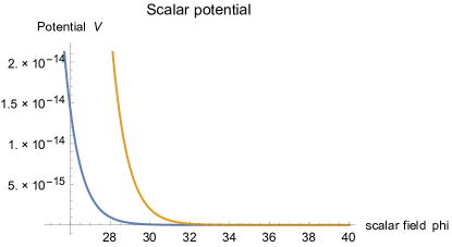
Figure 1: Behavior of the scalar potential as a function of the scalar field, given by Eq. (70). The blue solid line corresponds to $\rm m_{\phi}=5$ (dark energy), while the yellow solid line corresponds to $\rm m_{\phi}=14$ (dark matter).

On the other hand, the cosmological term for this scenario is

$$\rm\Lambda(t)=\frac{4\pi G\rho_{0}m_{\phi}}{\left[\left(b_{1}\Delta t+b_{2}\right)^{2}-1\right]}$$ (71)

which is a behavior that anisotropic universes exhibit. We can observe that the universe has a bigger expansion rate for $\rm m_{\phi}=14$ (which accounts for approximately $\rm 70\%$ in the total matter density for dust scenario) than for $\rm m_{\phi}=5$. The behavior of these functions can be seen in Fig. (2)

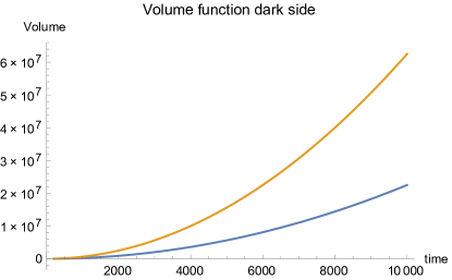
Figure 2: Behavior of the isotropic parameter (volume function) in the dust scenario, given by equation (65). Where we have set $\rm b_{1}=10,b_{2}=10,b_{0}=0.001$. The yellow solid line corresponds to $\rm m_{\phi}=14$ and the solid blue line corresponds to $\rm m_{\phi}=5$.

The time evolution for the average volume function in this scenario will be given by

$$\rm\eta^{3}=b_{0}\left[\left(b_{1}\Delta t+b_{2}\right)^{2}-1\right],$$ (72)

where $\rm b_{0}=\ell^{2}/(8\pi G\alpha_{\phi}\rho_{0})$ and $\rm b_{1}=(4\sqrt{3}\pi G\alpha_{\phi}\rho_{0})/\ell$, that in terms of the scalar field can be written as

$$\rm\eta^{3}=b_{0}sinh^{2}\left[\frac{1}{2}\sqrt{\frac{3}{2}\left(1+\frac{1}{m_{\phi}}\right)}\Delta\phi\right],$$ (73)

where we have used

$$\rm u=b_{1}t+b_{2}=cosh\left[\frac{1}{2}\sqrt{\frac{3}{2}\left(1+\frac{1}{m_{\phi}}\right)}\Delta\phi\right].$$

From the previous equation we can infer that the volume function has a stronger dependence on the dark scenario. We can see that for early times the value of $\rm m_{\phi}$ is small having a growing behavior; but when $\rm m_{\phi}$ has large values the volume function has decelerate behavior.

III.4 Anisotropic parameters

In anisotropic cosmology, the Hubble parameter $\rm H$ is defined in analogy with the FRW cosmology:

$$\rm H=\frac{\dot{a}}{a}=\frac{\dot{\eta}}{\eta}=\frac{1}{3}\left(H_{x}+H_{y}+H_{z}\right),$$ (74)

where $\rm H_{x}=\frac{\dot{a}_{1}}{a_{1}}$, $\rm H_{y}=\frac{\dot{a}_{2}}{a_{2}}$, and $\rm H_{z}=\frac{\dot{a}_{3}}{a_{3}}$.

The scalar expansion $\rm\theta$, shear scalar $\rm\sigma^{2}$ and the average anisotropic parameter $\rm\overline{A}_{m}$ are defined as

$$\rm\theta=\sum_{i=1}^{3}\frac{\dot{a}_{i}}{a_{i}}=3H,\qquad\sigma^{2}=\frac{1}{2}\left(\sum_{i=1}^{3}H_{i}^{2}-\frac{1}{3}\theta^{2}\right),\qquad\overline{A}_{m}=\rm\frac{1}{3}\sum_{i=1}^{3}\left(\frac{H_{i}-H}{H}\right)^{2},$$ (75)

respectively.

Using the results for the average scale factor $\eta$ and the dimensionless anisotropic functions $\rm m_{i}$, the average anisotropic parameter is $\rm\overline{A}_{m}=\frac{1}{3}\frac{\sum_{i=1}^{3}\ell_{i}^{2}}{\eta^{6}\left(\frac{\dot{\eta}}{\eta}\right)^{2}}=\frac{3\sum_{i=1}^{3}\ell_{i}^{2}}{4b_{0}^{2}b_{1}^{2}\,u^{2}}$, which can be written in terms of the scalar field using the variable u defined previously,

$$\rm\overline{A}_{m}=\frac{3\sum_{i=1}^{3}\ell_{i}^{2}}{4b_{0}^{2}b_{1}^{2}}\,Sech^{2}\left[\frac{1}{2}\sqrt{\frac{3}{2}\left(1+\frac{1}{m_{\phi}}\right)}\Delta\phi\right].$$ (76)

This parameter goes to zero for $\phi\to\infty$, causing the isotropization of the model. The other parameters aquire the form

$$\rm\theta = \rm 3\frac{\dot{\eta}}{\eta}=2b_{1}\frac{u}{u^{2}-1},$$ (77)

$$\rm\sigma^{2} = \rm\frac{1}{2}\left(\frac{\dot{m}_{i}}{m_{i}}\right)^{2}=\frac{1}{2}\frac{\sum_{i=1}^{3}\ell_{i}^{2}}{\eta^{6}}=\frac{1}{2}\frac{\sum_{i=1}^{3}\ell_{i}^{2}}{b_{0}^{2}(u^{2}-1)^{2}},$$ (78)

Following (Pradhan et al., 2011) and references therein, where the authors precise that the red-shift studies place the limit $\frac{\sigma}{\theta}\leq 0.3$ on the ratio of shear $\sigma$ to Hubble constant H in the neighborhood of our Galaxy today in order to have a sufficiently isotropic cosmological model, we obtain,

$$\rm\frac{\sigma^{2}}{\theta^{2}}=\frac{\sum_{i=1}^{3}\ell_{i}^{2}}{8b_{0}^{2}b_{1}^{2}}\,\frac{1}{u^{2}}=\frac{\sum_{i=1}^{3}\ell_{i}^{2}}{8b_{0}^{2}b_{1}^{2}}Sech^{2}\left[\frac{1}{2}\sqrt{\frac{3}{2}\left(1+\frac{1}{m_{\phi}}\right)}\Delta\phi\right].$$ (79)

Hence, we must have, $\rm\Delta\phi\leq\frac{2}{\sqrt{\frac{3}{2}\left(1+\frac{1}{m_{\phi}}\right)}}ArcSech\left(\frac{6\sqrt{2}b_{0}b_{1}}{10\sqrt{\sum_{i=1}^{3}\ell_{i}^{2}}}\right)$, where we consider that the constants should be fixed by the observational data, following the procedure in reference (Goswami et al., 2020). Using this result, the average anisotropic parameter is $\rm\overline{A}_{m}\leq 0.54$, see equations (75) and (79).

IV Conclusions and remarks

In this work we have characterized a sufficiently isotropic universe presenting a volume accelerated expansion in a dust stage, introducing a combination of results using two different approaches within an anisotropic cosmological model.

Employing a Misner-like transformation we can consider a decomposition into isotropic and anisotropic parts, where the properties of the latter are preserved, appearing as constraint equations (see (8)). Also, we extend the identification $\rm V(\phi)=2\Lambda$, (with $\Lambda$ a constant), to the dynamical case $\rm V(\phi(t))=2\Lambda(t)$.

The other idea was to consider a law between the energy density of the scalar field and that of the ordinary matter as follows: $\rm\rho_{\phi}=m_{\phi}\rho$; which results as a consequence of considering barotropic equations of state, $\rm P_{\phi}=\omega_{\phi}\rho_{\phi}$ and $\rm p=\gamma\rho$, and the equality of the corresponding barotropic indices. We found that for the solutions to the EKG equations to be consistent, the barotropic parameters must be equal.

We were able to find analytical solutions for the gravitational potentials and for the scalar field in a dust scenario, using the scaling solutions (previously found) between the energy density of the scalar field and that of the standard matter. It is worth mentioning that, in a dust scenario, the gravitational potentials have the same structure independently of wether or not the scalar field is taken into account: $\alpha_{\phi}=1$ without scalar field; $\rm\alpha_{\phi}=1+m_{\phi}$ with scalar field. We remark that parameter $\rm m_{\phi}$ is responsible for the description of the dark side of the universe, where $\rm m_{\phi}=5$ accounts for dark matter and $\rm m_{\phi}=14$ for dark energy. Considering this two values for the evolution of the universe, it turns out that for $\rm m_{\phi}=14$ the growth of the volume is faster than for $\rm m_{\phi}=5$, as expected, as shown in Fig. (2). The exact solution for the isotropic volume shows that the volume of the universe suffers an accelerated growth (in the dust scenario). Also, we found that (for the dust stage) the anisotropic Bianchi type I cosmological model evolves into the isotropic flat FRW model. This is supported by the fact that the anistropic parameters $\rm m_{i}$ acquire constant values for $t\to\infty$. Furthermore, the average anisotropy parameter $\rm\overline{A}_{m}$ is asymptotically null. Additionally, by considering the bound $\frac{\sigma}{\theta}\leq 0.3$, parameter $\rm\overline{A}_{m}$ was constrained to $\rm\overline{A}_{m}\leq 0.54$, which is consistent with the form considered in (Amirhashchi, 2018).

Finally, we remark that our findings indicate (regarding our toy model) that for the universe to present a volume accelerated expansion today, considering the volume deceleration parameter (68) (Tripathy et al., 2012), and the scalar potential must behaves as a hyperbolic cosecant, as shown in Fig. (1), implying that $\Lambda(t)\sim 1/t^{2}$. We also would like to note that we could not find this type of potential in the literature regarding studies in scalar field anisotropic cosmology.

References

• Abdel (1990) Abdel A.M.M.: Gen. Rel. Grav. 22, 655 (1990).
• Arbab & Abdel (1994) Arbab, A.I., & Abdel-Rahaman, A.M.M.: Phys. Rev. D 50, 7725 (1994).
• Akarsu et al. (2019) Akarsu, Ö., et al.: Phys. Rev. D 100, 023532 (2019).
• Amirhashchi (2018) Amirhashchi, H.: Phys. Rev. D 97, 063515 (2018).
• Amirhashchi (2019) Amirhashchi, H. & Amirhashchi, S.: Phys. Rev. D 99, 023516 (2019).
• Arbad (1997) Arbab, A.I.: Gen. Rel. Grav. 29, 61 (1997).
• Arbad (2001) Arbab, A.I.: Spacetime and substance 1, 39 (2001).
• Arbad (2003) Arbab, A.I.: Class. Quantum Grav. 20, 93 (2003).
• Arbad (2004) Arbab, A.I.: Astrophys. Space Sci. 291, 141 (2004).
• Aroonkumar (1993) Aroonkumar Beesham.: Phys. Rev. D 48, 3539 (1993).
• Aroonkumar (1994) Aroonkumar Beesham.: Gen. Rel. Grav. 26, 159 (1994).
• Bal & Singh (2008) Bal, R., & Singh, J.P.: Int. J. of Theor. Phys. 47, 3288 (2008).
• Bali & Jain (2002) Bali, R., & Jain, V.C.: Pramana J. Phys. 59, 1 (2002).
• Bali (2011) Bali, R.: Int. J. of Theor. Phys. 50, 3043 (2011).
• Belinchon (2008) Belinchón, J.A.: Int. J. Mod. Phys. A 23, 5021 (2008).
• Belinskii & Khalatnikov (1972) Belinskii, V.A., & Khalatnikov, I.M.: Sov. Phys. JETP 63, 1121 (1972).
• Birkel & Sarkar (1997) Birkel, M., & Sarkar, S.: Astropart. Phys. 6, 197 (1997).
• Burd (1988) Burd, A.B., & Barrow, J.D., Nucl. Phys. B 308, 929 (1988).
• Bylan & Scialom (1998) Bylan, S.,& Scialom, D.: Phys. Rev. D 57, 6065 (1998).
• Carneiro & Lima (2005) Carneiro, S., & Lima, J.A.S.: Int. J. Mod. Phys. A 20, 2465 (2005).
• Carvalho et al. (1992) Carvalho, J.C. et al.: Phys. Rev. D 46, 2404 (1992).
• Copeland et al. (1998) Copeland, E.J. et al.: Phys. Rev. D 57, 4686 (1998).
• Cunha & Santos (2004) Cunha, J.V., & Santos, R.C.: Int. J. Mod. Phys. D 13, 1321 (2004).
• Chen & Wu (1990) Chen, W., & Wu, Y.S.: Phys. Rev. D 41,695 (1990).
• Espinoza et al (2014) Espinoza García, Abraham., et al.: Int. J. of Theor. Phys. 53 (9), 3066-3077 (2014)
• Esposito et al. (2007) Esposito, G., et al.: Class. Quantum Grav. 24, 6255 (2007).
• Ferreira & Joyce (1997) Ferreira, P.G., & Joyce, M., Phys. Rev. Lett. 79, 4740 (1997).
• Ferreira & Joyce (1998) Ferreira, P.G., & Joyce, M.: Phys. Rev. D 58, 023503 (1998).
• Folomeev & Gurovich (2000) Folomeev, V.N., & Gurovich, V. Ts.: Gen. Rel. Grav. 32(7), 1255 (2000).
• Fomin et al. (2005) Fomin, P.I., et al.: preprint [gr-qc/0509042].
• Goswami et al. (2020) Goswami, G.K., et al.: Mod. Phys. Let. A 2050086 (2020), https://doi.org/10.1142/S0217732320500868.
• Halliwell (1985) Halliwell, J.: Phys. Lett. B 185, 341 (1985).
• Jamil & Debnath (2011) Jamil, M., & Debnath, U.: Int. J. of Theor. Phys. 50, 1602 (2011).
• Kalligas et al. (1992) Kalligas, D. et al.: Gen. Rel. Grav. 24, 351 (1992).
• Knop et al. (2003) Knop R.A. et al.: Astrophys. J. 598, 102 (2003).
• Kumar & Singh (2007) Kumar, S., Singh, C.P.: Astrophys Space Sci 312, 57 (2007).
• Liddle & Sharrer (1998) Liddle, A.R., & Sharrer, R.J.: Phys. Rev. D 59, 023509 (1998).
• Lucchin & Matarrese (1985) Lucchin, F., & Matarrese, S.: Phys. Rev. D 32, 1316 (1985).
• Lima & Maia (1994) Lima, J.A.S., & Maia, J.M.F.: Phys. Rev. D 49, 5597 (1994).
• Lima & Carvalho (1994) Lima, J.A.S., & Carvalho, J.C.: Gen. Rel. Grav. 26, 909 (1994).
• Lima & Trodden (1996) Lima, J.A.S., & Trodden, M.: Phys. Rev. D 53, 4280 (1996).
• Martinez & Sanz (1995) Martinez-Gonzalez, E., & Sanz, J.L.: Astronomy and Astrophysics 300, 346 (1995).
• Mukhopadhyay et al. (2011) Mukhopadhyay, U. et al.: Int. J. of Theor. Phys. 50, 752 (2011).
• Overduin & Cooperstock (1998) Overduin, J.M., & Cooperstock, F.I.: Phys. Rev. D 58, 043506 (1998).
• Pavon (1991) Pavon, D.: Phys. Rev. D bf 43, 375 (1991).
• Perlmutter et al. (1999) Perlmutter, S. et al.: astrophys. J. 517, 565 (1999).
• Pradhan & Kumar (2001) Pradhan, A. & Kumar, A.: Int. J. of Mod. Phys. D 10, 291 (2001).
• Pradhan (2003) Pradhan, A.: Int. J. of Mod. Phys. D 12, 941 (2003).
• Pradhan (2007) Pradhan, A.: Fizika B 16, 205 (2007).
• Pradhan (2009) Pradhan, A.: Commun. Theor. Phys. 51, 367 (2009).
• Pradhan & Pandey (2003) Pradhan, A., & Pandey, A.P.: Int. J. of Mod. Phys. D 12, 1299 (2003).
• Pradhan & Pandey (2006) Pradhan, A., & Pandey, A.P.: Astrophys. and Spa. Sci. 301, 127 (2006).
• Pradhan et al. (2007) Pradhan, A. et al.: Int. J. of Theor. Phys. 46, 2774 (2007).
• Pradhan et al. (2007) Pradhan, A. et al.: Rom. J. Phys. 52, 445 (2007).
• Pradhan et al. (2008) Pradhan, A. et al.: Brazilian J. of Phys. 38, 167 (2008).
• Pradhan et al. (2011) Pradhan, A. et al.: Int. J. Theor. Phys. 50, 2923 (2011).
• Pradhan et al. (2012) Pradhan, A. et al.: Astrophys. Space Sci. 337, 401 (2012).
• Pradhan et al. (2015) Pradhan, A. et al.: Indian J. Phys. 89(5), 503 (2015).
• Rahman & Ansary (2013) Rahman, M.A., & Ansary, M.: Prespace time J. 4, 871 (2013).
• Ray et al. (2011) Ray, S. et al.: Int. J. of Theor. Phys. 50, 939 (2011).
• Riess et al. (1998) Riess, A.G., et al., astron. J. 116, 1009 (1998).
• Riess et al. (2004) Riess, A.G., et al.: Astrophys. J. 607, 665 (2004).
• Saha (2006) Saha, B.: Astrophys. and Spa. Sci. 302, 83 (2006).
• Shahalam et al. (2015) Shahalam, M. et al.: Eur. Phys. J. C 75, 395 (2015).
• Shen (2013) Shen, M.: Int. J. of Theor. Phys. 52, 178 (2013).
• Silveira & Waga (1997) Silveira V., & Waga, I.: Phys. Rev. D 56, 4625 (1997).
• Singh et al. (1998) Singh, T. et al.: Gen. Rel. Grav. 30, 573 (1998).
• Singh et al. (2008) Singh, J.P. et al.: Astrophys. Spa. Sci. 314, 83 (2008).
• Singh (2008) Singh, J.P., Astrophys Spa. Sci. 318, 103 (2008).
• Singh et al. (2013) Singh, M.K. et al.: Int. J. of Phys. 1, 77 (2013).
• Socorro et al. (2010) Socorro, J., et al.: Rev. Mex. Fís. 56(2), 166-171 (2010).
• Socorro et al. (2014) Socorro, J., et al.: Advances in High Energy Phys. 805164 (2014).
• Socorro et al. (2015) Socorro, J., et al.: Astrophys. Spa. Sci. 360, 20 (2015).
• Sola & Stefancic (2005) Sola, J., & Stefancic, H.: Phys. Lett. B 624, 147 (2005).
• Sola & Stefancic (2006) Sola, J., & Stefancic, H.: Mod. Phys. Lett. A 21, 479 (2006).
• Spergel et al. (2007) Spergel, D.N., et al.: Astrophys. J. Suppl. 170, 377 (2007).
• Starobinsky (1998) Starobinsky, A.A., JETP Letters 8, 757 (1998).
• Tegmark et al. (2004) Tegmark, M., et al.: Phys. Rev. D 69, 103501 (2004).
• Tripathy et al. (2012) Tripathy, S.K., et al.: Astrophys. Spa. Sci. 340, 211 (2012).
• Tripathy (2013) Tripathy, S.K., Int. J. Theor. Phys. 52, 4218 (2013).
• Vishwakarma (2000) Vishwakarma, R.G.: Class Quantum Grav. 17, 3833 (2000).
• Vishwakarma (2001) Vishwakarma, R.G.: Gen. Rel. Grav. 33, 1973 (2001).
• Wand et al. (1993) Wand, D. et al.. Ann (NY) Acad. Sci. 688, 647 (1993).
• Weetterich (1998) Weetterich, C.: Nucl. Phys. B 302, 668 (1998).
• Zia et al. (2019) Zia, R., et al: New Astronomy 72, 83 (2019).