Abstract

In this paper we present a detailed analysis of the Faraday depth (FD) spectrum and its clean components obtained through the application of the commonly used technique of Faraday rotation measure synthesis to analyze spectro-polarimetric data. In order to directly compare the Faraday depth spectrum with physical properties of a magneto-ionic medium, we generated synthetic broad-bandwidth spectro-polarimetric observations from magnetohydrodynamic (MHD) simulations of a transonic, isothermal, compressible turbulent medium. We find that correlated magnetic field structures give rise to a combination of spiky, localized peaks at certain FD values, and broad structures in the FD spectrum. Although the majority of these spiky FD structures appear narrow, giving an impression of a Faraday thin medium, we show that they arise from strong synchrotron emissivity at that FD. Strong emissivity at a FD can arise because of both strong spatially-local polarized synchrotron emissivity at a FD or accumulation of weaker emissions along the distance through a medium that have Faraday depths within half the width of the rotation measure spread function. Such a complex Faraday depth spectrum is a natural consequence of MHD turbulence when the lines of sight pass through a few turbulent cells. This therefore complicates the convention of attributing narrow FD peaks to presence of a Faraday rotating medium along the line of sight. Our work shows that it is difficult to extract the FD along a line of sight from the Faraday depth spectrum using standard methods for a turbulent medium in which synchrotron emission and Faraday rotation occur simultaneously.

xx 1 5 Received: date; Accepted: date; Published: date An In-depth Investigation of Faraday Depth Spectrum Using Synthetic Observations of Turbulent MHD Simulations Aritra Basu ¹*, Andrew Fletcher ², S. A. Mao ³, Blakesley Burkhart ^4,5, Rainer Beck ³, Dominic Schnitzeler ⁶ Aritra Basu, S. A. Mao, Andrew Fletcher, Blakesley Burkhart, Rainer Beck and Dominic Schnitzeler Correspondence: aritra@physik.uni-bielefeld.de

1 Introduction

The advent of broad-band receivers on all major radio telescopes in the last decade have opened up new avenues for investigating the properties of synchrotron-emitting relativistic plasma in astrophysical objects. Previously, one had to observe the same source at multiple, widely-spaced frequencies to understand its polarization behaviour. Broad-band radio spectro-polarimetric measurements of the Stokes $Q$ and $U$ parameters makes it possible to measure the variation of the polarized synchrotron emission over a wide contiguous frequency range which can provide crucial insights into the properties of the magneto-ionic medium for a large number of sources in a much reduced amount of observing time. Broad-band spectro-polarimetry has played a crucial role in unveiling the properties of magnetic fields in nearby galaxies (Mao et al., 2015; Damas-Segovia et al., 2016; Stein et al., 2019), in high redshift galaxies (Kim et al., 2016; Mao et al., 2017), in active galactic nuclei (AGN; O’Sullivan et al., 2012, 2017; Pasetto et al., 2018) and the intergalactic medium (O’Sullivan et al., 2019). In order to physically interpret such data, the technique of Faraday rotation measure (RM) synthesis (Burn, 1966; Brentjens and de Bruyn, 2005) and direct fitting of the Stokes $Q$ and $U$ spectra of a polarized source with models of the magneto-ionic media, known as Stokes $Q,U$ fitting (Farnsworth et al., 2011; O’Sullivan et al., 2012; Anderson et al., 2015) have been developed. It is often not straightforward to interpret the results from these techniques and connect them to the physical properties of the magnetized plasmas being investigated (Anderson et al., 2016).

Currently, several large-scale spectro-polarimetric campaigns are underway, mostly in the 1 to 5 GHz frequency range. On one hand, dedicated surveys with interferometers are being conducted to study the broad-band polarization properties of millions of extragalactic sources. For example, the Karl G. Jansky Very Large Array Sky Survey (VLASS; Myers et al., 2014; Lacy et al., 2019), the Polarization Sky Survey of the Universe’s Magnetism (POSSUM; Gaensler et al., 2010), the QU Observations at Cm wavelength with Km baselines using ATCA (QUOCKA), the MeerKAT International GHz Tiered Extragalactic Exploration (MIGHTEE) Survey (Jarvis et al., 2016), and the recent LOFAR Two-meter Sky Survey (LoTSS; Van Eck et al., 2018, 2019) and S-PASS/ATCA (Schnitzeler et al., 2019). Many more broad-band polarization surveys are planned in the future with the upcoming Square Kilometre Array (SKA).

On the other hand, to study the diffuse Galactic magneto-ionic medium, broad-band, large sky-area surveys below $\sim 15$ GHz with single dish telescopes have been undertaken, e.g., the Global Magneto-Ionic Medium Survey (GMIMS; Wolleben et al., 2009), the GALFA Continuum Transit Survey (GALFACTS; Taylor, 2013), the S-band Polarization All Sky Survey (S-PASS; Carretti et al., 2019), survey with the SKA-MPG prototype telescope (Basu et al., 2019), the C-Band All Sky Survey (C-BASS; Jones et al., 2018) and the Q-U-I JOint TEnerife (QUIJOTE; Génova-Santos et al., 2015a, b).

With these broad-band polarization surveys, pressing astrophysical problems, such as, black hole accretion and its connection to AGN jet launching mechanism, cosmic evolution of magnetic fields in galaxies, structure and strength of magnetic fields in the interstellar, intra-cluster and intergalactic medium will be investigated (see e.g. Bourke et al., 2015). In addition to addressing astrophysical questions, these surveys will also contribute to the solution of fundamental cosmological questions via sensitive measurements of the Galactic diffuse synchrotron emission. This emission contaminates cosmological signals from the early Universe, such as, the cosmic microwave background radiation, the cosmic dawn and the epoch of reionization.

Quantities related to the plasma properties of a magneto-ionic medium that can be derived from observations are: the intrinsic fractional polarization and angle of the linearly polarized synchrotron emission, the Faraday depth (FD) and its dispersion. The intrinsic fractional polarization is determined by the ratio of turbulent to ordered magnetic field strengths in the plane of the sky averaged over the telescope beam (Sokoloff et al., 1998). The intrinsic angle of the linearly polarized emission gives us information about the orientation of the ordered magnetic fields in the plane of the sky. The Faraday depth gives us information on the strength and direction of the average magnetic field parallel to the line of sight and its spatial variation can help us to distinguish between coherent and anisotropic random magnetic fields (Jaffe et al., 2010). The dispersion of FD depends upon the properties of turbulent magnetic fields parallel to the line of sight. Hence, robust measurements of these quantities can provide insights into the 3-dimensional properties of magneto-ionic media in astrophysical sources. To measure them, RM synthesis and Stokes $Q,U$ fitting techniques are applied to broad-band spectro-polarimetric observations. Therefore, it is imperative to investigate, in detail, the scope of application of these data analysis techniques and their limitations. Understanding the efficacy and efficiency of these tools are of paramount importance for the success of the above mentioned surveys.

In this paper we will focus on the technique of RM synthesis when it is applied to infer properties of diffuse medium, e.g., the Galactic interstellar medium (ISM). Starting with magnetohydrodynamic (MHD) simulations of isothermal, transonic, compressible turbulent plasma, similar to that observed in the Galactic ISM (Gaensler et al., 2011; Koley and Roy, 2019), we use ray-tracing to simulate broad-band spectro-polarimetric observations. Then, we apply RM synthesis to test what we can learn about the medium. The major questions we will investigate are: (1) Is there a difference in the nature of the Faraday depth spectrum obtained by applying RM synthesis to a medium with a realistic model of turbulence from MHD simulations versus the commonly used model of turbulence as a Gaussian random field? (2) What is the origin of complexity in the Faraday depth spectrum? (3) Can RM synthesis recover the Faraday depth of a diffuse medium which is simultaneously Faraday rotating and emitting polarized synchrotron radiation?

This paper is organized as follows. In Section 2 we discuss in brief the techniques of RM synthesis and Stokes $Q,U$ fitting. We present in brief the salient features of the software package, COSMIC, for generating synthetic broad-band spectro-polarimetric data from MHD simulations in Section 3. In Section 4 we test the numerical performance of COSMIC using simulated media for which the broad-band polarization behaviour is known analytically. We present details of the MHD simulations in Section 5 and synthetic polarization observations performed by applying COSMIC to the simulations are discussed in Section 6. In Section 7 we present a detailed analysis of the results obtained from RM synthesis and compare them to the intrinsic properties of the medium, and we summarize our findings in Section 8.

2 Common spectro-polarimetric data analysis techniques

RM synthesis and Stokes $Q,U$ fitting are two commonly used techniques that are used to extract information from broad-band observations of polarized emission. The parameters of interest are the intrinsic fractional polarization ($p_{\rm int}$), intrinsic orientation of the polarization angle ($\theta_{0}$), Faraday depth (FD) and the intrinsic dispersion of FD ($\sigma_{\rm FD}$). In order to gain physical insights into an astrophysical system, robust measurement of these quantities are essential.

$\bullet$ Stokes parameter ($Q,U$) fitting: The technique of Stokes $Q,U$ fitting is a parametric fitting of the Stokes $Q$ and $U$ parameters’ wavelength ($\lambda$) dependent variation using models of a turbulent magneto-ionic media analytically derived, for example, in Burn (1966), Tribble (1991), Sokoloff et al. (1998) and Rossetti et al. (2008), and therefore requires assumptions on the nature of the medium being investigated. In Stokes $Q,U$ fitting, $p_{\rm int}$, $\theta_{0}$, FD and $\sigma_{\rm FD}$ are directly fitted for as model parameters. However, fitting is limited to a set of source models that might oversimplify the physics inside real radio sources and their environments. Moreover, often the broad-band Stokes $Q$ and $U$ data cannot be fitted by a single model and therefore linear combinations of models are used. Since increasing the number of models improves the quality of the fit by increasing the number of free parameters (principle of parsimony; Anderson, 2007), statistical measures, such as, the Bayesian inference criterion and/or Akaike information criterion are used to limit the number of models or to choose between degenerate fits (O’Sullivan et al., 2012; Schnitzeler, 2018). However, Stokes $Q,U$ fitting has the advantage of also fitting for the spectral index of the polarized flux density (see Schnitzeler, 2018), which is not possible in RM synthesis and is one of the origins of complexity in the Faraday depth spectrum (e.g., Schnitzeler, 2018; Schnitzeler et al., 2019).

$\bullet$ Rotation measure synthesis: RM synthesis is a Fourier transform-like operation in which it is assumed that the linearly polarized radio source can be described as a sum of emitters at their respective Faraday depths, and is the Fourier transform of the frequency spectrum of the complex polarization (Burn, 1966; Brentjens and de Bruyn, 2005). Therefore, RM synthesis makes only a weak assumption about the physical properties of the magneto-ionic medium and is a non-parametric approach. Like any Fourier transform performed over a finite space (in this case a finite frequency coverage), the Faraday depth spectrum (variation of fractional polarization $p$ or polarized intensity $PI$ as a function of FD) obtained from RM synthesis is convolved with a complicated response function determined by the frequency coverage of the observations. The response function is known as the rotation measure spread function (RMSF) and has sidelobes due to sharp cut-offs and gaps in the frequency coverage. Artefacts produced by the RMSF sidelobes can be deconvolved by applying the technique of RM clean (Heald et al., 2009). In the case when Faraday rotation originates at multiple Faraday depths or Faraday depth varies contiguously through a volume, RM clean models a source as discrete $\delta$-function emitters in Faraday depth space known as clean components. The full-width at half-maximum (FWHM) of the RMSF is determined by the bandwidth in $\lambda^{2}$ of the observations and it determines how well the emitters can be resolved in the Faraday depth space. The channel width of observations determines the maximum observable FD and the highest frequency end determines the sensitivity to the largest scale structure in the Faraday depth space (see Brentjens and de Bruyn, 2005, for details). This means that the results depend heavily on the frequency coverage used, and interpreting the RM cleaned Faraday depth spectra or the clean components can be a challenging task.

Another challenge of RM synthesis is the way $p_{\rm int}$, $\theta_{0}$, FD and $\sigma_{\rm FD}$ are determined from the Faraday depth spectrum. This comes down to a matter of choice for an individual investigator. In order to extract information on the physical quantities of magneto-ionic media, attempts have recently been made to describe the Faraday depth spectrum using parametric functions. In such an approach, the Faraday depth spectrum is modelled as a $\delta$-function for a purely Faraday rotating medium, as a top-hat function for a simultaneously Faraday rotating and synchrotron emitting medium containing regular magnetic fields and constant densities of thermal and relativistic electrons, and as super-Gaussian function for a medium which contains both turbulent and regular magnetic fields (Anderson et al., 2016; Ideguchi et al., 2017, 2018). Recently, Van Eck (2018) proposed a model-free description of mapping the Faraday depth spectrum to polarized emission as a function of distance. The parametric descriptions, for both Faraday depth spectra and Stokes $Q,U$ fitting, implicitly assume a Gaussian random distribution of the components of the turbulent magnetic field. In contrast, the turbulent magnetic field and free electron distribution in the diffuse ISM, the focus of this paper, are expected to have spatially correlated structures, and are often non-Gaussian (Armstrong et al., 1995; Burkhart et al., 2009; Haverkorn et al., 2008; Hollins et al., 2017; Makarenko et al., 2018). Further, observations of extragalactic sources and the diffuse Galactic emission have revealed that FD spectra often show complicated structures (Anderson et al., 2016; Van Eck et al., 2017; Wolleben et al., 2019) referred to as Faraday complexity. A part of the complexity can be introduced by the spectral index of the polarized emission, and hence RM synthesis is typically performed on fractional polarized parameters. Dedicated efforts, both mathematical and computational, are required to incorporate information on spectral index and Faraday depolarization into RM synthesis.

Because of these caveats, it is necessary to investigate the results of RM synthesis using MHD turbulence simulations which provide a more realistic magnetic field and Faraday depth distribution that are not described by simple Gaussian statistics.

3 COSMIC: from physical quantities to Stokes parameters and Faraday rotation

We have developed an end-to-end, fully parallelized, Python based software package — Computerized Observations of Simulated MHD Inferred Cubes (COSMIC) — to generate synthetic data cubes of Stokes parameters as a function of frequency for further analysis. RM synthesis and RM clean are performed by integrating the pyrmsynth package into COSMIC. The code requires 3-dimensional (3-D) spatial cubes of the three magnetic field components (in units of $\mu$G) and the distribution of neutral or ionized gas density (in units of cm^-3) computed from MHD simulations as inputs, in a Cartesian coordinate system. Depending on the type of MHD simulations, other optional inputs can be provided, such as, the 3-D spatial distributions of temperature and the number density or energy spectrum of cosmic ray electrons (CREs). The default coordinate system is chosen such that the line of sight (LOS) is along the $z$-axis and, $x$- and $y$-axes are in the plane of the sky. However, COSMIC allows the user to choose the LOS axis perpendicular to any of the six faces of the cube.

For MHD simulations which do not contain cosmic rays, to compute the total synchrotron emission and the Stokes $Q$ and $U$ parameters of the linearly polarized synchrotron emission, a user can choose from several options to determine the number density of CREs ($n_{\rm CRE}$) and their energy spectrum. Similarly, to compute the Faraday depth, the number density of free electrons ($n_{\rm e}$) is estimated by choosing a suitable ionization model depending on the type of the simulations and other ancillary data computed in the simulations, such as, the gas temperature. Using these, COSMIC computes the 2-D distribution of the total synchrotron intensity and the Stokes $Q$ and $U$ parameters on the plane of the sky across a frequency range specified by the user. Details of how observables are computed numerically and the different user-specified options are presented in Appendix A.

4 Benchmarking COSMIC with analytic models of magneto-ionic media

To test the accuracy of the numerical calculations performed by COSMIC, we first compared outputs from it with simple models of magneto-ionic media whose frequency-dependent polarization behaviour have analytic solutions. We simulated two types of radio sources which are simultaneously synchrotron emitting and Faraday rotating: (1) a uniform slab containing a regular magnetic field and constant densities of free electrons and CREs (Burn, 1966; Sokoloff et al., 1998); (2) a volume that contains both regular and turbulent magnetic fields in which the turbulent fields have a Gaussian random distribution, known as the internal Faraday dispersion (IFD) model (Sokoloff et al., 1998).

Table 1: Setup parameters used to generate synthetic observations to test COSMIC with uniform slab and internal Faraday dispersion (IFD) models.

Parameter	Uniform slab	IFD
Regular field strengths	$\langle B_{x}\rangle=4\,\mu$G, $\langle B_{y}\rangle=7\,\mu$G, $\langle B_{z}\rangle=5\,\mu$G
Random field strengths:
$\sigma_{x}$ ($\mu$G)	0	10
$\sigma_{y}$ ($\mu$G)	0	10
$\sigma_{z}$ ($\mu$G)	0	10
$n_{\rm e}$ (cm-3)	0.05	0.05
Box size	$512\times 512\times 512\,{\rm pc^{3}}$
Mesh size	$1\times 1\times 1\,{\rm pc^{3}}$
Spectral index	$\alpha=-0.8$
Spectral curvature	None
Frequency range	$\nu_{\rm min}=0.5$ GHz, $\nu_{\rm max}=6$ GHz
Number of channels	$n_{\rm chan}=500$

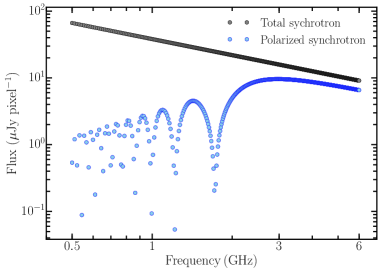
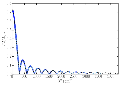
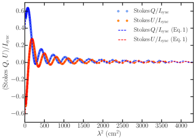
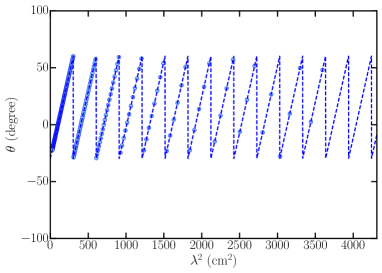
Figure 1: Synthetic spectra of Stokes parameters of synchrotron emission generated by COSMIC for a uniform slab. Numerically computed quantities are shown as the data points and the analytical functions for the linearly polarized quantities are shown as dashed lines. Top left: Spectrum of the total synchrotron flux density (grey points) and the linearly polarized flux density (blue points). Top right: Variation of the factional polarization with $\lambda^{2}$. Bottom left: Variation of fractional Stokes $Q$ and $U$ parameters as a function of $\lambda^{2}$. Bottom right: Variation of the angle of the plane of linear polarization ($\theta$) with $\lambda^{2}$.

4.1 Uniform slab model

A uniform slab, also commonly referred to as a ‘Burn slab’ after Burn (1966), is a synchrotron emitting medium in which the strengths of the three magnetic field components and the densities of CRE and thermal electrons are all spatially constant. We generated such a medium on a $512\times 512\times 512$ pixel³ mesh and assumed the mesh points to be separated by 1 pc. Therefore, the physical volume of the simulated uniform medium is $512\times 512\times 512$ pc³. The values of the physical quantities used to simulate a uniform slab are listed in Table 1. We have used CRE density such that the total synchrotron flux density of the medium is 10 Jy at 1 GHz (see Section A.1). We assumed a power-law energy spectrum of the CREs, so that, the synchrotron emission also follow a power-law frequency spectrum with spectral index $\alpha=-0.8$ ($I_{\nu}\propto\nu^{\alpha}$, where $I_{\nu}$ is the intensity at frequency $\nu$).

For such a medium, the complex fractional polarization varies with wavelength $\lambda$ as (Burn, 1966; Sokoloff et al., 1998),

$$p(\lambda)=p_{\rm int}\,\dfrac{\sin{\rm FD}\,\lambda^{2}}{{\rm FD}\,\lambda^{2}}\,{\rm e}^{2\,i\,\left(\theta_{0}+\frac{1}{2}\,{\rm FD}\,\lambda^{2}\right)}.$$ (1)

Here, $p_{\rm int}$ is the intrinsic fractional polarization of the medium, after accounting for any frequency-independent beam depolarization of the synchrotron emission that might be present, for example due to unresolved turbulent magnetic fields. As there is no beam or random magnetic field in this model, $p_{\rm int}$ is the same as the maximum fractional polarization $p_{\rm max}$ given in Eq. (10). The expected values of $p_{\rm int}$, FD and $\theta_{0}$ are listed in Table 2.

Spectra of the total and linearly polarized synchrotron flux densities, $I_{\rm sync}$ and $PI$, respectively, obtained from COSMIC for a single LOS through the domain are shown in the top-left panel in Fig. 1. The top-right and bottom-left panels in Fig. 1 show the fractional Stokes parameters, i.e., $PI/I_{\rm sync}$, and $Q/I_{\rm sync}$ and $U/I_{\rm sync}$, respectively, as a function of $\lambda^{2}$, computed from the data using Eqs. (6), (14), (15) and (16). The bottom-right panel show the variation of the polarization angle, $\theta_{0}$, with $\lambda^{2}$. The dashed lines in Fig. 1 show the analytical function given by Eq. (1). To check the robustness of our numerical calculations, the parameters of the analytical model, namely, $p_{\rm int}$, FD and $\theta_{0}$, were calculated directly from the COSMIC output. Note that the fractional polarization and the angle of polarization are given by the amplitude and phase of the complex polarization, and are dependent on the wavelength (e.g., Eq. 1). Therefore, $p_{\rm int}$ and $\theta_{0}$ can either be determined at $\lambda=0$, which is unphysical, or when FD and/or $\sigma_{\rm FD}$ are $0~{}\rm rad\,m^{-2}$. We therefore computed $p_{\rm int}$ and $\theta_{0}$ by setting FD in each pixel of the 3-D cube to zero and then performing the synthetic observations. In Table 2, we present the expected values of $p_{\rm int}$, FD and $\theta_{0}$, and compare them with those computed from the cubes. All the values are in excellent agreement with the theoretical values.

Table 2: Expected values of physical parameters for the setup parameters used in Table 1 and values obtained using COSMIC.

Parameter		Uniform slab			IFD
		Expected	Obtained		Expected	Obtained
$p_{\rm int}$		0.73	0.73		0.176	0.174
FD ($\rm rad\,m^{-2}$)		$103.94$	$103.94$		103.94	103.63
$\sigma_{\rm FD}$ ($\rm rad\,m^{-2}$)		0.0	0.0		9.20	9.18
$\theta_{0}$ (∘)		$150.26$	$150.25$		150.26	150.25

4.2 Internal dispersion model

The internal Faraday dispersion (IFD) model describes a medium that is simultaneously synchrotron emitting and Faraday rotating in the presence of both regular and random magnetic fields, wherein the random field is isotropic, has Gaussian statistics and is delta-correlated (i.e. there are no correlated structures in the field). In other words, the correlation length is same as the length of the mesh point separation. We generated a volume of the same dimension as in Section 4.1, but in this case, the magnetic field strengths of each component in each 1 pc³ pixel were drawn at random from a Gaussian distribution. The mean value of the Gaussian represents the regular field strength along the corresponding direction and the standard deviation is a measure of the strength of the turbulent fields. Values of the different parameters used to generate the IFD volume are listed in Table 1.

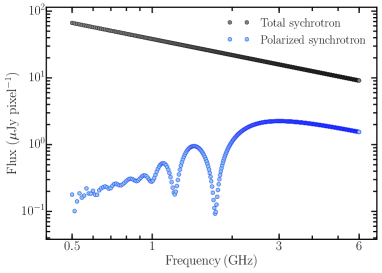
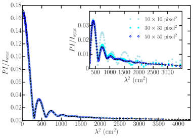
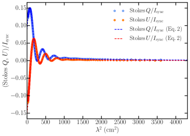
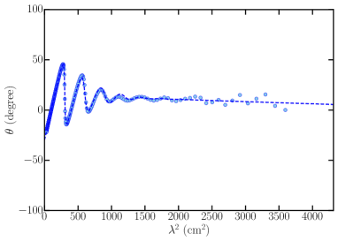
Figure 2: Synthetic spectra of Stokes parameters of synchrotron emission generated by COSMIC for an internal Faraday dispersion model. Different shades of data points in the inset of the top right panel show the fractional polarization computed by averaging over different areas. All other panels, data points and lines have the same meaning as in Fig. 1. In the main plots only the results for averaging over $50\times 50~{}\rm pixel^{2}$ are shown.

The complex fractional polarization in such a medium varies with $\lambda$ as (Sokoloff et al., 1998),

$$p(\lambda)=p_{\rm int}\,{\rm e}^{2i\theta_{0}}\,\left(\dfrac{1\,-\,\exp[-(2\,\sigma_{\rm FD}^{2}\,\lambda^{4}-2\,i\,{\rm FD}\,\lambda^{2})]}{2\,\sigma_{\rm FD}^{2}\,\lambda^{4}-2\,i\,{\rm FD}\,\lambda^{2}}\right).$$ (2)

Here, $\sigma_{\rm FD}$ is the intrinsic dispersion of FD and is given by (Beck, 2007),

$$\sigma_{\rm FD}=0.812\,\langle n_{\rm e}\rangle\,\sigma_{\rm\|}\,\sqrt{\dfrac{l_{0}\,L}{f_{\rm V}}},$$ (3)

where $\sigma_{\rm\|}$ is the strength of turbulent magnetic fields along the line of sight, $l_{0}$ is the correlation length of the product $n_{\rm e}\,\sigma_{\|}$, $L=512$ pc is the path-length through the magneto-ionic medium, and $f_{\rm V}$ is the volume filling factor of $n_{\rm e}$. In this example, since $n_{\rm e}$ is constant, $f_{\rm V}=1$, and $l_{0}=1$ pc as the random field is delta-correlated.

The intrinsic fractional linear polarization ($p_{\rm int}$) of the synchrotron emission originating from superposition of regular and isotropic random magnetic fields, and constant number density of CREs, is given by (Sokoloff et al., 1998),

$$p_{\rm int}=p_{\rm max}\,\dfrac{\langle B_{\perp}\rangle^{2}}{\langle B_{\perp}\rangle^{2}+\sigma_{x}^{2}+\sigma_{y}^{2}}.$$ (4)

For our choice of parameters in Table 1, $p_{\rm int}$, $\theta_{0}$, FD and $\sigma_{\rm FD}$ are theoretically expected to be 0.176, 150.26^∘, $103.94~{}\rm rad\,m^{-2}$ and $9.2~{}\rm rad\,m^{-2}$, respectively. In Table 2, we compare these values with those directly obtained from COSMIC output using the same method as described at the end of the previous section. The values agree well with each other. In Fig. 2, we show the variation of polarization fraction with $\lambda$ computed from synthetic observations of the simulated volume and they agree well with the analytic function given in Eq. (2).

We should point out that, in this case, we determined the frequency spectra of the polarization parameters shown in Fig. 2 by averaging over $50\times 50$ pixels² in the $I$, $Q$ and $U$ images. This is done to ensure that there are a sufficient number of pixels to capture the Gaussian statistics generated by standard routines for generating random numbers in Python. For smaller averaging areas, significant deviations of the synthetic data from the analytic function is observed, especially towards longer wavelengths. A comparison of the variation of fractional polarization with $\lambda^{2}$ obtained from synthetic observations by averaging over different areas is shown in the inset of the top right-hand panel of Fig. 2. At shorter wavelengths, all synthetic observations agrees well with the analytic function.

5 Applying COSMIC to MHD simulations of a turbulent medium

The magnetic fields and free electrons in the ISM have more complicated distributions than can be described by simple delta-correlated Gaussian statistics, for example they can have spatial correlations in their structure (see e.g., Haverkorn et al., 2008; Mao et al., 2015; Makarenko et al., 2018). Therefore, investigating the broad-band properties of the linearly polarized synchrotron emission from realistic MHD simulations is required, especially with several on-going and upcoming polarization surveys of the Milky Way’s diffuse emission.

Here we apply COSMIC to MHD simulations of isothermal, compressible and transonic turbulence in the ISM from Burkhart et al. Burkhart et al. (2009, 2013). Polarization observations of the Galactic plane and Galactic Hi 21 cm observations of the warm gas have confirmed the transonic nature of turbulence in the ISM (Gaensler et al., 2011; Herron et al., 2016; Koley and Roy, 2019). The simulation set up is similar to that of past works (Kowal et al., 2007; Burkhart et al., 2009; Bialy et al., 2017). We refer to these works for the details of the numerical set-up and we only provide a short overview here. The simulation used here is a 3-D turbulent box of isothermal compressible MHD turbulence with a resolution $512^{3}$, and each mesh point is separated by 1 pc. The code is a third-order accurate essentially nonoscillatory scheme which solves the ideal MHD equations in a periodic box with purely solenoidal driving of the flow at a scale $2.5$ times smaller than the domain size, i.e., $\sim 200$ pc. The simulation has two control parameters: the sonic Mach number ($M_{\rm s}=v/c_{\rm s}$, where $v$ is the flow velocity and $c_{\rm s}$ is the sound speed) and Alfvénic Mach number ($M_{\rm A}=v/v_{\rm A}$, where $v_{\rm A}$ is the Alfvén speed). In these simulations, we used $M_{\rm s}\approx 2.0$ and $M_{\rm A}\approx 0.7$. The magnetic field consists of a regular background field ($B_{\rm ext}$) and a turbulent field ($b$), i.e., $B=B_{\rm ext}+b$ with the magnetic field initialized along a single preferred direction. In the choice of our coordinate system, the regular field is along the $x$-direction and has a strength of $10\,\mu$G. This regular field will not contribute to Faraday depth as the LOS is along the $z$-direction.

The distribution of the strengths of the three magnetic field components over the entire simulation volume is shown in Fig. 3. The corresponding dashed lines are for equivalent Gaussian distributions computed from the mean and standard deviation of the corresponding field component. The distribution of $B_{x}$ shows deviation from a Gaussian distribution, while that for $B_{y}$ and $B_{z}$ agrees well with Gaussian distributions. We must stress, although the distributions of the magnetic field components closely resembles a Gaussian distribution, spatially they are correlated on the driving scale of turbulence in these simulations, unlike the delta-correlated Gaussian fields described in Section 4.2. For details regarding their structural and statistical properties we refer interested readers to Burkhart et al. (Burkhart et al., 2009, 2013). To summarize, physical specifications of the simulations are as follows: (1) Physical size of the simulation volume is $512\times 512\times 512$ pc³. (2) Mesh resolution of the simulation is $1\times 1\times 1$ pc³. (3) The mean magnetic field strengths are: $\langle B_{x}\rangle=10\,\mu$G and $\langle B_{y}\rangle=\langle B_{z}\rangle\approx 0\,\mu$G; and the three components have dispersions $\sigma_{x}=2\,\mu$G, $\sigma_{y}=3\,\mu$G and $\sigma_{z}=3\,\mu$G. Thus, the ratio of regular to turbulent field strengths in this simulation is $\sim 2$. We would like to emphasize that this regular field, local to the simulated volume, would only contribute to the polarized intensity of the synthetic observations, unlike those observed in external galaxies. Polarization measurements in external galaxies are performed with comparatively lower spatial resolution. Therefore, they are are mostly sensitive to the ordered component of the magnetic field within the beam, or to the large-scale regular fields, and therefore in external galaxies, the ordered fields are found to be about three times weaker than the turbulent fields (Fletcher, 2010).

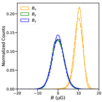
Figure 3: Distribution of strengths of the three components of the magnetic field from the isothermal, compressible turbulence simulations used for our analysis are shown as the histograms. The dashed lines show Gaussian distributions with mean and standard deviation computed from the corresponding field component.

As the MHD simulation used in this work is isothermal and in thermal equilibrium, the ionization fraction, $f_{\rm ion}$, of neutral hydrogen is assumed to be constant throughout the volume and can be chosen to compute the free electron density $n_{\rm e}$ (see Appendix A.2). Increasing $f_{\rm ion}$ increases $n_{\rm e}$ and thereby the amount of Faraday rotation ($\rm FD_{cell}$) in each cell of the MHD cube, which increases the amount of Faraday depolarization through the entire LOS. To find physically motivated value for $f_{\rm ion}$, we produced maps of emission measure (${\rm EM}=\int n_{\rm e}^{2}\,{\rm d}l$) and dispersion measure (${\rm DM}=\int n_{\rm e}\,{\rm d}l$) for various values of $f_{\rm ion}$ and compared EM vs. DM by averaging over different areas (Schnitzler, 2008). In the left-hand panel of Fig. 4 we show the variation of EM as a function of DM. The slope of the best-fit line (shown as the black line) is found to be $2.4\pm 0.1$ indicating that the simulation used here is strongly clumpy with low $f_{\rm V}$. We varied $f_{\rm ion}$ such that the amplitude roughly matches with observations of the Galactic ISM. For example, Berkhuijsen and Müller (2008) found a slope of 1.15 for the EM vs. DM relation for the diffuse ionized gas around the Solar neighbourhood with mean $f_{\rm V}=0.08$. In denser and clumpier ISM with $f_{\rm V}<0.06$, the slope of the EM vs. DM relation was estimated to be 2 by Pynzar’ (2016).

For the simulations used here, the amplitude of the EM vs. DM relation agrees well with that observed in our Galaxy for $f_{\rm ion}=0.5$ (see Fig. 4). In the right-hand panel of Fig. 4, we show the distribution of $n_{\rm e}$ in the simulation volume for $f_{\rm ion}=0.5$. Here, the median $n_{\rm e}$ is $0.11~{}{\rm cm^{-3}}$ and it has a maximum value of $3.5~{}{\rm cm^{-3}}$. Such values of $n_{\rm e}$ are typically observed within Galactic latitudes $\pm 15^{\circ}$ (Cordes and Lazio, 2003; Pynzar’, 2016). The distribution of $n_{\rm e}$ is well approximated by a Gamma distribution (solid black line) with shape parameter $\approx 2.25$ and inverse scale parameter $\approx 0.06$, i.e., an expectation value for $n_{\rm e}\approx 0.13~{}\rm cm^{-3}$.

For the values of $n_{\rm e}$ and $B_{\|}$ in these MHD simulations, $<0.3\%$ of the $1~{}{\rm pc^{3}}$ mesh points have $|{\rm FD_{cell}}|>3~{}{\rm rad\,m^{-2}}$ and $<1\%$ mesh points have $|{\rm FD_{cell}}|>2~{}{\rm rad\,m^{-2}}$. That means, within the cell, $<0.3\%$ and $<1\%$ of the mesh points undergo Faraday depolarization of $>20\%$ and $>10\%$, respectively, at frequencies below $\sim 0.5$ GHz. Calculations of the polarization parameters in COSMIC assumes that the Faraday depolarization in a single mesh point is negligible (see Appendices A.2, A.3 and A.4). Therefore, for these simulations COSMIC can be safely applied to frequencies above 0.5 GHz.

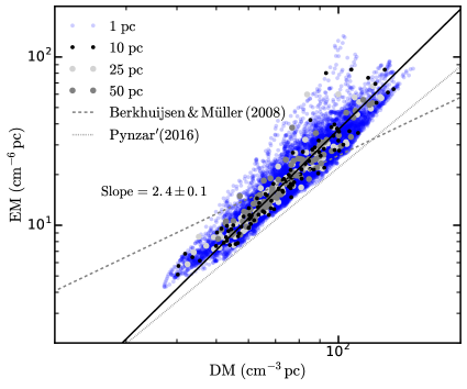
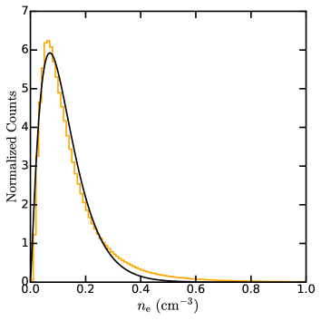
Figure 4: Left: Variation of emission measure (EM) as a function of dispersion measure (DM) for an ionization fraction of 0.5 of the simulation volume. The different shades for the symbols represents different averaging scales. The black line shows the best-fit, and the grey dashed and dotted lines are from Berkhuijsen and Müller (2008) and Pynzar’ (2016), respectively. Right: Distribution of free electron density $n_{\rm e}$ in the simulation volume. The solid black line shows the best-fit gamma function representation of the distribution.

The following options were used to compute the synthetic spectra of $I_{\rm sync}$, $PI$, Stokes $Q$ and $U$ in the rest of this paper. (1) As the simulations do not contain cosmic rays and the typical CRE propagation lengths are expected to be comparable to or larger than the size of the simulation box (see Appendix A.1), we assume that the CREs are uniformly distributed throughout the 3-D volume of the simulation. (2) The CREs follow a power-law energy spectra with the same energy index throughout the volume. Thus, the synchrotron intensity spectral index ($\alpha$) is constant, both spatially and with frequency, with $\alpha=-0.8$ defined as $I_{\rm sync}\propto\nu^{\alpha}$. (3) $n_{\rm CRE}$ is normalized such that the total synchrotron flux density at 1 GHz integrated over the entire volume is 10 Jy (see Appendix A.1). Note that the amplitude of the frequency spectrum of intrinsic emissivities of the total synchrotron emission, and Stokes $Q$ and $U$ parameters can be scaled depending on the unknown $n_{\rm CRE}$ without affecting the relative frequency variation. (4) The ionization fraction is constant throughout the volume with $f_{\rm ion}=0.5$.

In the following analyses, we have not added any systematic effects arising from combining data observed using multiple telescope receivers into one large bandwidth or telescope noise. Also, the synthetic observations are not sampled using $u-v$ coverage of an interferometer and therefore mimicks observations performed using a single dish radio telescope. This is because we want to investigate what can be learnt about a medium from RM synthesis under ideal conditions.

6 Synthetic observations of MHD simulations

We compute synthetic spectra of the total and linearly polarized quantities that describe the synchrotron emission of the volume in the frequency range 0.5 to 6 GHz divided into 500 frequency channels. The choice of lowest frequency is determined by the need to minimize Faraday depolarization within each 3-D mesh point (see Section 5) and the highest frequency is chosen such that the synthetic observations are sensitive to broad structures in the Faraday depth space and roughly corresponds to the high frequency end of on-going spectro-polarimetric surveys of the diffuse Galactic synchrotron emission (e.g. Jones et al., 2018).

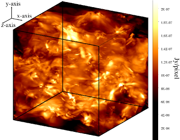
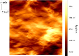
Figure 5: Left: 3-D synchrotron emissivity per pixel at 1 GHz. Synchrotron emissivity was computed assuming a constant density of CREs throughout the 3-D volume. Right: 2-D synchrotron intensity at 1 GHz integrated along $z$-axis.

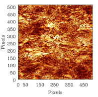
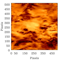
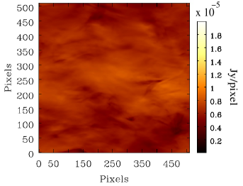
Figure 6: Linearly polarized intensities at 0.5 GHz (left), 1.5 GHz (middle) and 5 GHz (right) including the effects of Faraday depolarization.

In the left-hand panel of Fig. 5, we show the 3-D total synchrotron emissivity of the simulated volume at 1 GHz. The right-hand panel shows the projected 2-D map of the total synchrotron intensity ($I_{\rm sync}$) obtained by integrating the 3-D cube in the left-hand panel along the $z$-axis, our LOS axis. Since we have assumed a constant density of CREs, all of the structure in this image arises due to the variations of synchrotron emissivity caused by fluctuations of the magnetic field component in the plane of the sky, both along and across the LOS.

In Fig. 6, we show the polarized intensities at 0.5, 1.5 and 5 GHz. Due to frequency dependent Faraday depolarization, the polarized emission develops small-scale structures at lower frequencies. This is due to fluctuations in $B_{\|}$ along and across the lines of sight. For frequencies below $\sim 3$ GHz, where most of the polarized surveys of Galactic diffuse emission have been performed (e.g., Duncan et al., 1997; Wolleben et al., 2006; Testori et al., 2008; Wolleben et al., 2019), the polarized emission shows some ‘canal-like’ small scale structures (e.g. Shukurov and Berkhuijsen, 2003). Due to severe Faraday depolarization at 0.5 GHz, the polarized emission show structures on scales of a few pixels. The maps of Stokes $Q$ and $U$ parameters also show a similar trend in their structural properties with frequency. This underlines the challenge of combining interferometric observations of diffuse emission at different frequencies. The smooth, diffuse structure in Stokes $Q$ and $U$ at the highest frequencies will be filtered out from the data. This does not happen at lower frequencies because different sightlines undergo different amounts of Faraday depolarization, leading to rapid variations on small scales. This issue cannot be overcome even if frequency-scaled interferometer arrays are used to match the $u-v$ coverage at different frequencies.

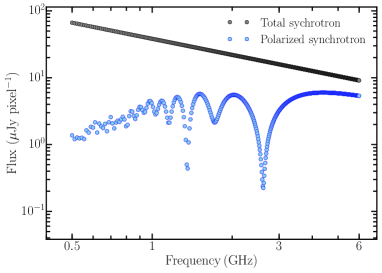
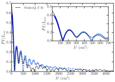
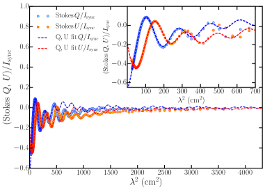
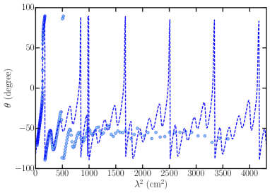
Figure 7: Synthetic spectra of Stokes parameters of synchrotron emission generated by COSMIC from MHD simulations. Here we have used $\alpha=-0.8$ and assumed optically thin synchrotron emission. Quantities computed from COSMIC are shown as the data points. Top left: Spectrum of the total synchrotron intensity is shown as the grey points and the linearly polarized intensity is shown as the blue points. Top right: Variation of the factional polarization with $\lambda^{2}$. Bottom left: Variation of Stokes $Q/I_{\rm sync}$ and $U/I_{\rm sync}$ parameters as a function of $\lambda^{2}$. Bottom right: Variation of the angle of the plane of linear polarization ($\theta$) with $\lambda^{2}$. All the dashed lines represents the best-fit obtained from Stokes $Q,U$ fitting. The insets shows the wavelength regime below $700$ cm² within which successful fits were obtained (see text for details).

6.1 Broad-band spectra of Stokes parameters

Fig. 7 shows the synthetic spectra of the total synchrotron emission and parameters of linearly polarized synchrotron emission between 0.5 and 6 GHz. All the quantities are computed by averaging over a randomly chosen $30\times 30$ pixel² region corresponding to a spatial scale of $30\times 30$ pc². The polarized emission at lower frequencies ($<1$ GHz) show strong frequency-dependent variations. This implies that at low frequencies, the small-scale polarized structures seen in the left-hand panel of Fig. 7 are also expected to vary strongly with slight changes in frequency.

Although Stokes $Q,U$ fitting is not the main focus of this work, we none-the-less present in brief the result of fitting the synthetic data shown in Fig. 7. Stokes $Q,U$ fitting was performed using analytical functions for several types of depolarization models described in Sokoloff et al. (1998) and O’Sullivan et al. (2017) and their linear combinations. In our Stokes $Q,U$ fitting routine, we allow combination of a maximum of three depolarization models and use the corrected Akaike information criteria (Hurvich and Tsai, 1989; Cavanaugh, 1997) to choose the best-fit model. Because of the strong variation of the Stokes $Q$ and $U$ parameters in the longer wavelength regime (in this case roughly $>700$ cm² corresponding to frequencies $<1.1$ GHz), the combination of three depolarization models is not sufficient to fit the Stokes $Q$ and $U$ parameter spectra for the entire wavelength range considered here. However, for wavelengths below $700$ cm², fits converged successfully (inset in Fig. 7). For the synthetic data in Fig. 7, the best-fit was obtained with a linear combination of three internal Faraday depolarization components (Eq. 2). In fact, none of the regions we have investigated in these simulations could be fitted by a single depolarization model, in contrast to the simulated volumes in Section 4. This implies that spatially correlated distributions of the magnetic fields and/or thermal electron densities, as in these MHD simulations, could possibly give rise to multiple polarized components (also see Section 7.2) that have different wavelength-dependent depolarization behaviours.

The failure of Stokes $Q,U$ fitting in being able to fit the synthetic data below $\sim 1$ GHz with three or less components brings to light an important aspect about the technique. To our knowledge, most of the Stokes $Q,U$ fitting in the literature has been applied to data above $\sim 1$ GHz, or to high redshift sources for which the rest-frame emission originated close to 1 GHz or higher, and up to three polarization components has been sufficient to fit those data. It will be interesting to investigate the performance of Stokes $Q,U$ fitting when broad-band spectro-polarimetric data is acquired below 1 GHz for a large number of sources with future surveys. A detailed investigation of the results of Stokes $Q,U$ fitting, the generic properties of the method in connection to different types of MHD simulations and the optimum number of depolarization models required to extract maximum physical insights into a diffuse magneto-ionic medium is beyond the scope of this paper, and will be discussed elsewhere.

6.2 Reconstructed Faraday depth map

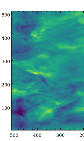
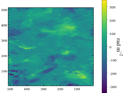
Figure 8: Comparison of the Faraday depth map computed from the MHD simulations (left) with the Faraday depth map reconstructed from RM synthesis applied to synthetic observations in the frequency range 0.5 to 6 GHz (right).

To construct the Faraday depth map from the synthetic Stokes $Q$ and $U$ parameters, we applied the technique of RM synthesis. In order to avoid complications arising from the effects of spectral index (Schnitzeler, 2018; Schnitzeler et al., 2019), all analysis pertaining to RM synthesis were performed on fractional polarization quantities, i.e., $q=Q/I_{\rm sync}$, $u=U/I_{\rm sync}$ and $p=PI/I_{\rm sync}$. For the frequency setup used here, the RMSF has a FWHM of $10~{}\rm rad\,m^{-2}$ and is sensitive to extended Faraday depth structures up to $\sim 1250~{}\rm rad\,m^{-2}$ (see Brentjens and de Bruyn, 2005). This is sufficient to perform high Faraday depth resolution investigation of these synthetic observations without being affected by missing large-scale Faraday depth structures.

The Faraday depth spectrum was computed for the search range $-3000$ to $+3000$ $\rm rad\,m^{-2}$ with a step size of $0.5~{}\rm rad\,m^{-2}$. Since we have not added any noise to the synthetic data, RM clean was performed by setting loop gain to 0.02 and with 1000 cleaning iterations. This allows cleaning down to the minimum fractional emissivity of the 3-D mesh points in the simulated volume. Synthetic observations are processed using the pyrmsynth implementation of RM synthesis to produce a Faraday depth spectrum which is then deconvolved using RM clean. In Fig. 8, we show the expected Faraday depth map from the MHD simulations (${\rm FD_{MHD}}=0.812\,\int\,n_{\rm e}\,B_{\|}\,{\rm d}l$, computed using Eq. (9)) on the left-hand side and the reconstructed Faraday depth map computed using RM synthesis ($\rm FD_{RM\,synthesis}$) on the right-hand side. We have determined $\rm FD_{RM\,synthesis}$ in a pixel as the location of the peak of the Faraday depth spectrum computed by fitting a parabola. The spatial features in the reconstructed FD map broadly matches with the ${\rm FD_{MHD}}$ map, but the magnitudes differ significantly. Also, some regions of the reconstructed FD map show sharp jumps across neighbouring pixels. In the next section we will discuss in detail the complexity of determining the Faraday depth from the Faraday depth spectrum.

In the left-hand panel of Fig. 9, we show the distribution of the difference $\rm FD_{RM\,synthesis}-FD_{\rm MHD}$. The FWHM of the RMSF for the synthetic observations of only $10~{}\rm rad\,m^{-2}$, which in combination with the signal-to-noise ratio, gives an estimate of the error of determined FD. Since, we have not added any noise to the synthetic data, the estimated $\rm FD_{RM\,synthesis}$ is expected to have vanishing error. However, $\rm FD_{RM\,synthesis}$ is significantly off with respect to the expected $\rm FD_{\rm MHD}$ by up to $\pm 200~{}\rm rad\,m^{-2}$. This is mainly because of the way FD is determined from Faraday depth spectra that are highly complex as discussed in the next section. To assess possible systematic effects arising from the RMSF and/or sensitivity to large Faraday depth structures, we also computed $\rm FD_{RM\,synthesis}$ for different frequency coverages. The different histograms in Fig. 9 (left-hand panel) show the distribution of $\rm FD_{RM\,synthesis}-FD_{\rm MHD}$ for the different frequency coverages. The respective RMSFs are shown in the right-hand panel of Fig. 9. For none of the frequency ranges is FD recovered with sufficient accuracy.

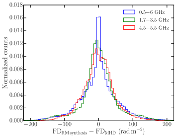
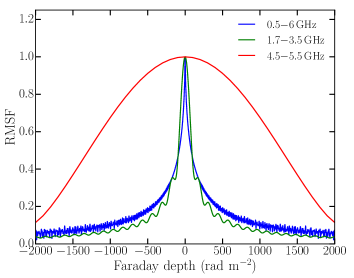
Figure 9: Left: Distribution of the difference between FD estimated by applying RM synthesis ($\rm FD_{RM\,synthesis}$) and the FD obtained from the MHD simulation ($\rm FD_{\rm MHD}$) computed using Eq. (9). The different colours for the histograms are for different frequency coverages. Right: RMSF for the corresponding frequency coverages shown in the left-hand panel.

7 Comparing Faraday depth spectrum obtained by RM synthesis with the intrinsic spectrum of a turbulent medium

In this section we examine Faraday depth spectrum of individual lines of sight through both the simple benchmark data cubes of Section 4 and the MHD turbulence data cube described in Section 5, using two different methods. First, the COSMIC code is used to generate Stokes $Q$ and $U$ values using the observational setup described in Section 6 and Faraday depth spectra were computed in the same way described in Section 6.2. Second, we calculate the polarized emissivity and the local Faraday depth at each position along the same lines of sight to generate a model of the intrinsic Faraday depth spectrum for that LOS.

We wish to know how close the two Faraday depth spectra are for a realistic model of a turbulent, synchrotron emitting medium. In particular, does a spectrum obtained by RM synthesis give a true representation of the emissivity distribution by Faraday depth that the medium actually produces? If the answer to this is no, then what is the connection between the Faraday depth spectrum and the physical state of the emitting region? Whilst the answers to these questions will probably not be surprising, with hindsight, to someone familiar with the method, we will gain valuable insights into the nature of the problem from this investigation.

7.1 Faraday depth spectra of analytical models

We first illustrate the process using the two simple models for the distribution of emissivity and Faraday depth described in Section 4: a uniform slab and a internal Faraday dispersion volume with delta-correlated Gaussian random fields. Artefacts introduced by the RM synthesis and RM clean algorithms will be clearly visible, the data will provide a useful reference point for comparisons later, and we shall begin to see the difficulties in discriminating between very different sources using the technique.

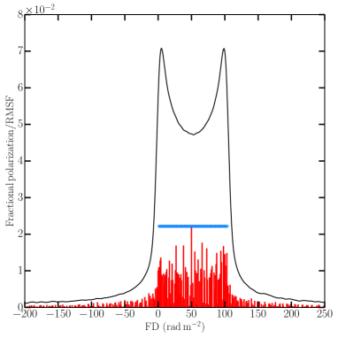
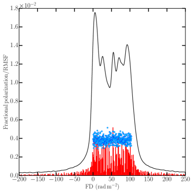
Figure 10: Faraday depth spectra for the uniform slab (left) and internal Faraday dispersion (IFD) models (right). The red lines are the clean components. The blue dots shows the relative intrinsic synchrotron emissivities at respective FD computed from the simulated volume described in Section 4 and represents a model of the intrinsic Faraday depth spectrum. For the IFD model, we have averaged $10\times 10~{}{\rm pixel}^{2}$ pixels.

In Fig. 10, for both the uniform slab and Gaussian random field models, we show three different versions of the Faraday depth spectra along a single LOS: the continuous lines show the RM cleaned Faraday depth spectrum; the vertical red lines show the position and amplitude of individual clean components in this spectrum selected by the RM clean algorithm; the blue dots show the polarized emission at each Faraday depth computed directly from the simulations and serves as a model Faraday depth spectrum. At $\lambda=0$, the last representation is equivalent to equation 2 in Van Eck (2018).

For the uniform slab (Fig. 10, left-hand panel), the Faraday depth spectrum for a single LOS shows the double-horn feature that arises due to sharp edges in the magnetic field distribution and finite frequency coverage for performing RM synthesis (see e.g., Frick et al., 2011; Beck et al., 2012; Schnitzeler et al., 2015, for detailed discussions). One of the peaks is close to 0 $\rm rad\,m^{-2}$, while the other peak is located at $102.1~{}\rm rad\,m^{-2}$, consistent with the Faraday depth through the entire layer of $103.94~{}\rm rad\,m^{-2}$. The Faraday depth spectrum for the IFD model (Fig. 10, right-hand panel) also shows peaks in the spectrum from the front of the layer at $0~{}\rm rad\,m^{-2}$ and the rear at $~{}100~{}\rm rad\,m^{-2}$, but three additional maxima are detected by RM synthesis. It is worth noting that all 512 mesh points along this LOS have a random magnetic field component which is not correlated with the magnetic field of its neighbours (the random field is said to be delta-correlated). These random fluctuations will produce point-to-point, uncorrelated, variation in both the polarized emissivity and the local Faraday depth, as seen for the blue points in Fig. 10 (right-hand panel). The reason why there are a few, not 512 peaks, in the spectrum is because these local variations are blended together by both the resolution of the RMSF (see right-hand panel of Fig. 9) and because emission from different positions along the LOS may occur at the same Faraday depth. In principle, the former effect can be removed by deconvolution using RM clean but the latter effect is irreversible. It is important to note, a single LOS through an IFD medium does not contain sufficient statistical information on the delta-correlated random fields, therefore in Fig. 10 (right-hand panel) we have averaged over $10\times 10~{}\rm pixel^{2}$. For a comparison with single LOS results presented later as closely as possible, we have chosen averaging over $10\times 10~{}\rm pixel^{2}$ instead of larger area as was done in Section 4.

The blue points in Fig. 10 show the intrinsic Faraday depth spectra of the models, which should be compared to the red bars showing the components selected by RM clean. The only noticeable difference between the distribution of clean components, which are roughly constant in each model, is the lower amplitudes for the random field model which is a consequence of lower intrinsic fractional polarization (Eq. 4). The Faraday depth spectra allow for an easy identification of the uniform slab, but the clean components do not. In both models the amplitudes of the clean components appear to be systematically lower than the intrinsic emissivities because of normalization: the peak intrinsic emissivity is scaled to be the same magnitude as the peak clean component, as described in Section 7.3.

7.2 The origin of complexity in the Faraday depth spectrum of a turbulent medium

Here, we look into the Faraday depth spectrum obtained by performing RM synthesis on the synthetic observations of MHD turbulence simulations and compare them to features in the variations of synchrotron emissivity and Faraday depth along the LOS. We will discuss based on three LOS shown in Fig. 11, as they are sufficiently representative of any other LOS and are therefore general representation of the results we will present. The left column displays $B_{\perp}^{(1-\alpha)}=B_{\perp}^{1.8}$ (for $\alpha=-0.8$), which is directly proportional to the linearly polarized synchrotron emissivity, at each position along the LOS and also the Faraday depth from that position to the front of the domain (the side nearest to the notional observer). The emissivity-proxy fluctuates randomly about the expected mean value of $\langle B_{\perp}\rangle^{(1-\alpha)}={(\langle B_{x}\rangle^{2}+\langle B_{y}\rangle^{2})}^{(1.8)/2}\approx(10\,\mu{\rm G})^{1.8}$ (see Section 5), due to variation in $B_{x},B_{y}$. This will translate into random structure in the amplitude of the Faraday depth spectrum. In Fig. 11 (left column), $B_{\perp}^{(1-\alpha)}$ is colourized based on the intrinsic angle of polarization. Because of the strong $B_{\rm ext}$ along the $x$-direction, the polarization angle do not show strong fluctuations.

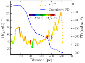
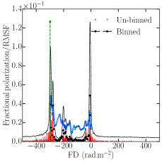
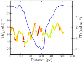
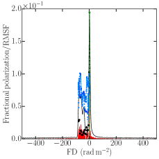
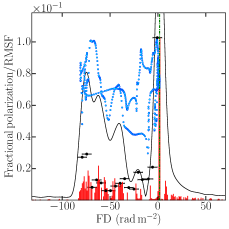
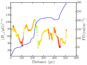
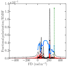
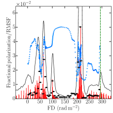
Figure 11: Left: Variation of $B_{\perp}$ (circles) and cumulative FD (blue line) with distance along three random LOS each of which is one pixel wide. $B_{\perp}$ is coloured based on the angle of the polarized synchrotron emission. Middle: Faraday depth spectrum for the corresponding LOS. The blue points show the local polarized emissivity at that FD. The red lines are the clean FD components and the green dot-dashed line is located at the FD along that LOS. The black points show the summed linearly polarized synchrotron emissivity per FD bin of size half the RMSF. The amplitudes of the polarized emissivities are normalized to the peak FD clean component. Right: Same as the middle-panel zoomed around the peak of the Faraday depth spectrum for a clearer visualization.

The Faraday depth of each point along the LOS shows a systematic non-random variation with position. This is because the Faraday depth is cumulative from a given position to the observer and the fluctuations in the magnetic field components are not delta-correlated. The correlation scale of $L_{\rm c}\sim 200$ pc is controlled by the forcing used to drive turbulence in the simulation: in these simulations the forcing scale is about 2.5 times smaller than the simulation box (Burkhart et al., 2009). The driven turbulence contains fluctuations on all scales from $L_{\rm c}$ down to the dissipation scale (the separation between mesh points in this case), but the power-law behaviour of the magnetic energy means that the field is strongest at $L_{\rm c}$. So, the Faraday depth builds up systematically over path lengths of roughly 200 pc. An interesting consequence of this is that, because the domain size is 512 pc, the Faraday depth variation along the LOS is not necessarily a monotonic function: the maximum magnitude of Faraday depth along a given LOS may not be that from the back to the front of the domain. If the domain was half the size, the Faraday depth variation would tend to be monotonic and if it were much bigger we would see multiple peaks and troughs in the Faraday depth variation. For domain sizes $L\gg L_{\rm c}$, FD variations would eventually appear to be random for $\langle B_{\|}\rangle=0~{}\mu$G. Thus, the form of the intrinsic Faraday depth variation depends on the number of turbulent cells along the LOS and does not necessarily look like a random function for shorter path-lengths. However, when combined with the variations in emissivity to produce the intrinsic Faraday depth spectrum the smoothness in ${\rm FD}$ along the LOS is not translated into a smooth spectrum.

The intrinsic polarized emissivity and Faraday depth combine to give the intrinsic Faraday depth spectrum shown by the blue points in the middle and right columns of Fig. 11. Note that these have been normalized to the maximum RM clean component, so only the relative variation contains useful information. Also shown in these panels is the spectrum obtained by RM synthesis and its clean components. The Faraday depth spectra are highly complex with multiple peaks and clean components referred to as a “Faraday forest” by Beck et al. (2012). These spectra are also clearly different from that obtained using delta-correlated Gaussian random field as an approximation to turbulence shown in Fig. 10 (right-hand panel).

It is clear that the Faraday depth spectra are also very different from the intrinsic model spectra. RM synthesis tends to select a few strong peaks which are not always the FD along the entire LOS, nor are they closely related to features in the intrinsic polarized emission. This illustrates a fundamental difficulty in interpreting RM synthesis data. It may be wrong to interpret some of the narrow, high peaks as the action of a Faraday screen, or a Faraday-thin component: a region in which there is no polarized emission, but which produces Faraday rotation. However, the corresponding left panels show that there is emission from all locations along the LOS.

A further difficulty in interpretation arises because the maximum absolute value of the Faraday depth along a LOS is not necessarily the Faraday depth through the entire box. The latter is shown by the green dash-dot line in the middle and right columns of Fig. 11. For example, in the first row of Fig. 11 the spectrum obtained by RM synthesis has strong peaks at $\rm FD\approx 0$ and $\rm FD\approx-300~{}\rm rad\,m^{-2}$ and looking at the left panel we see these correspond respectively to the emission generated at the front and back of the LOS. However, in the second row, the emission that produces the strong spectral peak near $\rm FD=0~{}\rm rad\,m^{-2}$ comes from emission from both the front and back of the layer. The Faraday depth through the entire layer is $\rm FD=1.67~{}\rm rad\,m^{-2}$ and the maximum along this LOS, $\rm FD\approx-80~{}\rm rad\,m^{-2}$ originates from the middle. There is no way yet, that we are aware of, to reliably recover any of the true properties of the Faraday depth along the LOS from the Faraday depth spectrum alone. Images produced using the strongest spectral peak or the maximum absolute FD as proxies for some assumed property of a source, such as, its intrinsic polarized emissivity or the total Faraday depth through it, may be misleading.

Pronounced peaks in the Faraday depth spectrum of a synchrotron emitting medium can arise in two ways. A strong peak in emissivity from a region where the FD is changing slowly over a small distance will produce a narrow FD feature: an example is in the third row of Fig. 11, where the strong emission from a distance between 190 and 210 pc, where the FD profile shows a step-like feature, produces the spectral peak at $\rm FD\approx 100~{}\rm rad\,m^{-2}$. Alternatively, when the FD is constant, or changing slowly over large distances, comparatively weaker emission builds up at this FD and results in a peak in the spectrum: in the third row of Fig. 11 we see that $\rm FD\approx 200~{}rad\,m^{-2}$ between the distance $250$ and $450$ pc along the LOS, producing a pronounced peak at this FD in the spectrum. Such a scenario can occur when the angle of the polarized emission is changing slowly with distance. In neither case does a strong peak in the spectrum result from a Faraday screen. Whilst the origin of some spectral peaks can be approximately described by one of these mechanisms, there are also many peaks whose origin is not so simple and are discussed in the next section.

Multiple polarized components in Faraday depth spectrum is a natural consequence when the LOS passes through a few coherent scales. We believe, in the case when the LOS traverse through statistically large (asymptotically infinite) number of turbulent cells, Faraday depth spectrum similar to that obtained for delta-correlated random fields could perhaps be obtained. Given the typical driving scale of turbulence in the ISM, e.g., $\sim 50\textrm{--}100$ pc when driven by supernova (Armstrong et al., 1995; Elmegreen and Scalo, 2004), and the typical length of LOS through the ISM of a few kiloparsec, achieving such a limit is highly unlikely. Unfortunately, the MHD simulations used here do not allow us to test this scenario. At present we are not aware of any reliable method which can be used to interpret Faraday depth spectra that originate in a turbulent, synchrotron emitting region. Since turbulence and cosmic ray electrons are thought to be present throughout the ISM this problem requires careful investigation.

7.3 Comparing clean components to the intrinsic Faraday depth spectrum

In Fig. 11, the blue points showing the intrinsic emission at each Faraday depth are present between the main peaks in the spectra obtained by RM synthesis and RM clean. This is because, structures in FD are smoothed by the RMSF. In order to make a better comparison between the observed and intrinsic spectra it is important to consider the number of emitters in a given range of Faraday depths that is compatible with the resolution of the RMSF. We therefore binned synchrotron emissivities within a range of FD, with the bin-size determined by the RMSF. In our case, we used the bin-size $\Delta\textrm{FD}=\textrm{RMSF}/2$. The choice of this bin-size is motivated by the fact that we wanted to Nyquist sample the RMSF. This is equivalent to the sum of polarized intensities ($\varepsilon_{\rm bin}$) arising in the range $\rm FD\pm\Delta{\rm FD}/2$ and $\varepsilon_{\rm bin}$ is given by,

$$\varepsilon_{\rm bin}({\rm FD})=\sum\limits_{{\rm FD}_{i}}\,\varepsilon({\rm FD}_{i})\equiv N_{\rm bin}\,\langle\varepsilon_{\rm bin}\rangle,~{}\textrm{where}~{}{\rm FD}_{i}\in[{\rm FD-\Delta FD/2,FD+\Delta FD/2}].$$ (5)

Here, $N_{\rm bin}$ is the number of synchrotron emitting elements within a FD bin computed from the simulation and $\langle\varepsilon_{\rm bin}\rangle$ is the mean polarized synchrotron emissivity of that FD bin. As the intrinsic polarization angle of the synchrotron emission do not fluctuate strongly (as can be seen by the smooth colour variation of the angle of the polarized synchrotron emission in the left column of Fig. 11), simple addition of the polarized emissivities will not affect our conclusions. The black points in the middle and right columns of Fig. 11 show $\varepsilon_{\rm bin}$ located at the mean FD of the corresponding bin with the maximum value of $\varepsilon_{\rm bin}$ normalized to the peak value of the FD clean components. It is clear from the middle and the right-hand panels of Fig. 11 that the sum of polarized emission in FD bins captures the RM clean components, including their relative amplitudes, remarkably well.

Note that, strong $\varepsilon_{\rm bin}$, and thus a peak in the Faraday depth spectrum can originate either due to — (1) strong emissivity at a location along the LOS (large $\langle\varepsilon_{\rm bin}\rangle$), or due to (2) build up from several weaker emissions that have FD within $\pm\rm{RMSF}/4$ (large $N_{\rm bin}$). In fact, both these scenarios can occur along the same LOS. For example, in the top row of Fig. 11, the peak near $-300~{}\rm rad\,m^{-2}$ originates due to the first case, while the peak near $0~{}\rm rad\,m^{-2}$ is because of the second case. In the second row of Fig. 11, the peak near $0~{}\rm rad\,m^{-2}$ is a consequence of the second case although the polarized emission in that FD bin originate from both front and back of the sightline. This clearly demonstrates that, for a turbulent magneto-ionic medium which is simultaneously synchrotron emitting and Faraday rotating, a peak in the Faraday depth spectrum corresponds to the polarized emission summed roughly within $\pm\rm RMSF/4$, which necessarily may not arise from regions along the LOS that are spatially continuous. Therefore, special care must be taken when interpreting FD maps constructed through RM synthesis and relating them to the FD of the emitting volume, especially when the Faraday depth spectrum appears to be well resolved.

This brings out the important fact that, even if a broad-band observation is sensitive to extended structures in Faraday depth space and can resolve them, as our synthetic observations are, the RMSF plays an important role in determining the amplitudes of the clean components. Moreover, when performing RM synthesis for diffuse emissions, sharp peaks in the Faraday depth spectrum that are consistent with the width of the RMSF do not necessarily imply the presence of a Faraday rotating screen in the foreground of a synchrotron emitting volume.

Our investigation on Faraday depth spectra is based on a diffuse isothermal magneto-ionic medium as a representative Galactic ISM that contains transonic compressible turbulence. It is possible that the conditions of turbulence in different parts of the Galactic magneto-ionic medium could be of different type, including the distribution and direction of the regular magnetic fields. The conclusions regarding the origin of Faraday complexity and various peaks in the Faraday depth spectrum are expected to be general. However, depending on the spatial smoothness of the turbulent fields (for example, sub- or super-sonic turbulence) and strength of the regular fields, the peaks in Faraday depth spectrum could become smoother or merge together. In other words, the clumpyness of a well resolved Faraday depth spectrum could provide hints on the nature of turbulence in a magneto-ionic medium. Therefore, quantifications of the shape of Faraday depth spectrum beyond the recently used skewness and kurtosis (Ideguchi et al., 2017) is necessary to be investigated to distinguish between different types of turbulent medium.

8 Conclusions

We have investigated in detail various features in Faraday depth spectra obtained from synthetic broad-band spectro-polarimetric observations in the frequency range 0.5 to 6 GHz sampled with 500 frequency channels. We have developed a new software package, COSMIC, wherein a user can freely choose from several possible options to generate synthetic observations. In this work the synthetic observations were obtained from MHD simulations of an isothermal, transonic, compressible turbulence in a plasma, similar to that observed in the Galactic ISM. For comparison, we have also studied the Faraday depth spectrum for a simple delta-correlated Gaussian random description of turbulent magnetic fields. We reach the following conclusions:

1. For the MHD simulations used, Faraday depth varies smoothly with distance along the lines of sight due to spatially correlated structures in the magnetic field. Faraday depth varies on scales of $\sim 200$ pc, similar to the driving scale of turbulence in the simulations used in this work.

2. Strong Faraday depolarization at long wavelengths gives rise to canal-like small-scale structures in the polarized synchrotron emission. At the resolution of the MHD simulations used here, the polarized synchrotron emission below $\sim 1$ GHz shows spatial variation on few pixel scales that correspond to few parsecs.

3. For the choice of our frequency coverage, the synthetic observations are sensitive to structures extended up to $\sim 1250~{}\rm rad\,m^{-2}$ in Faraday depth space and resolve them with RMSF of $10~{}\rm rad\,m^{-2}$. This allowed us to perform a high resolution investigation of Faraday depth spectra. Faraday depth spectra for a medium containing Gaussian random magnetic fields that are delta-correlated are significantly different in structure as compared to those obtained from MHD simulations of a medium containing random magnetic fields that are spatially correlated. The latter is expected to be a closer representation of the diffuse ISM.

4. Faraday depth spectra of individual sightlines through the MHD cube show a combination of narrow and broad features, which cannot be described as a linear combination of simple models that are typically used when polarization data are analysed. The narrow structures are mostly consistent with the width of the RMSF containing a single FD clean component, typically considered as a signature of a medium that is only Faraday rotating, although the entire simulation volume is emitting synchrotron radiation.

5. We find that, modelling RM clean components of the Faraday depth spectrum as discrete emitters along a line of sight where, at a physical distance, the synchrotron emissivity of the emitters is located at the Faraday depth to that distance does not represent the clean components obtained from RM clean.

6. The clean components and their relative emissivities obtained from RM clean are well represented by the sum of polarized synchrotron emissivity in a Faraday depth bin of bin-size $\rm RMSF/2$.

7. Since the Faraday depth spectrum depends on the interplay of the emissivity $\varepsilon_{\rm sync}$ and the local Faraday depth, the complicated structures in Faraday depth can be explained as follows:
   – Strong sharp peaks in the spectrum can be produced due to reasons: (i) strong $\varepsilon_{\rm sync}$ at a single FD, or, (ii) build up of weaker $\varepsilon_{\rm sync}$ over a range of distance, not necessarily continuous, that have roughly constant FD, or whose FD lies in the range $\rm FD-RMSF/4$ and $\rm FD+RMSF/4$.
   – Broad spectral features are produced by: (iii) a gradient in FD at a constant $\varepsilon_{\rm sync}$. Deviations from “constant” $\varepsilon_{\rm sync}$ or FD produce sub-structure on (ii) and (iii).

8. Our analysis shows that it is highly non-trivial to infer the Faraday depths, i.e. the integral $0.812\,\int n_{\rm e}\,B_{\|}\,{\rm d}l$ along the entire LOS, for a diffuse medium that emits synchrotron radiation if turbulent magnetic fields are dominant.

The turbulent magneto-ionic medium in a real astrophysical source is expected to be further complicated as compared to our simplified assumptions on its properties, such as, a constant density of CREs having constant power-law spectral energy distribution, a constant ionization fraction of the neutral gas and above all, an ideal telescope response. In such scenarios, the generality of our investigation regarding peaks in Faraday depth spectrum originating due to accumulation of synchrotron emissivity within a range of FD determined by the RMSF is expected to hold true. The complication stems from the fact that, whether the stronger synchrotron emissivity is a consequence of magnetic fields alone or due to variations in density of CREs or due to variations in their energy spectrum, will remain degenerate. In the presence of telescope systematics and noise, complications can be even more difficult to disentangle. With several upcoming broad-band spectro-polarimetric surveys of the diffuse Galactic emission and other surveys for extragalactic sources that are targeting major astrophysical questions, interpreting results obtained from spectro-polarimetric data analysis techniques in general, and RM synthesis technique in particular, requires improved statistical methods.

All authors discussed and conceptualized this work; A.B. developed the software COSMIC based on a basic version by A.F.; B.B. performed the MHD simulations; A.B. performed all the analyses; and A.B. and A.F. wrote the paper. All authors discussed the interpretations of the results.

Appendix A Computerized Observations of Simulated MHD Inferred Cubes: COSMIC

Here, we discuss the details of numerical calculations performed by COSMIC to generate synthetic observations. COSMIC uses MHD simulation generated cubes in Cartesian coordinate system and assumes the $z$-axis as the default line of sight axis. However, any of the perpendicular axis of the six faces of the cube can be chosen by the user as the line of sight axis. In the following, we will present our calculations in the default coordinate system.

A.1 Synchrotron emissivity

The cubes of $B_{x}$ and $B_{y}$ are used to compute the magnetic field strength in the plane of the sky, $B_{\perp}=(B_{x}^{2}+B_{y}^{2})^{1/2}$, which is used to compute the synchrotron emissivity, $\varepsilon_{\rm sync}$, at a frequency $\nu$ in each cell as,

$$\varepsilon_{\mathrm{sync},\nu}=N_{0}\,n_{\rm CRE}\,B_{\perp}^{1-\alpha}\,\nu^{\alpha}\,\dfrac{{\rm e}^{-(\nu/\nu_{\rm c})}}{[1\,+\,(\nu/\nu_{\rm br})^{\gamma}]}.$$ (6)

Here, $n_{\rm CRE}$ is the number density of CRE, $N_{0}$ is an arbitrary normalization factor, $\alpha$ is the spectral index of the synchrotron emission, $\gamma$ is the spectral curvature parameter, and $\nu_{\rm br}$ and $\nu_{\rm c}$ defines the position of a break and cut-off frequency in the synchrotron spectrum.

Although some MHD simulations do include cosmic rays, here we apply COSMIC to a MHD simulation which does not have information on cosmic ray electrons, i.e., effects of their propagation and energy losses. In the scenario when $n_{\rm CRE}$ is unavailable, synchrotron emissivity is computed using one of the following assumptions:
(1) Constant $n_{\rm CRE}$ throughout the 3-D spatial cube.
(2) Cosmic rays follow local energy equipartition per mesh point, such that, $n_{\rm CRE}=B_{x}^{2}+B_{y}^{2}+B_{z}^{2}$. We note, however, that such a distribution of CRE is likely to be unphysical as equipartition conditions are unlikely to hold on small scales (Seta and Beck, 2019).
(3) Cosmic rays follows energy equipartition over an user defined volume such that, $n_{\rm CRE}=\sigma_{x}^{2}+\sigma_{y}^{2}+\sigma_{z}^{2}$, where $\sigma_{x,y,z}$ are the root mean square of the $x$, $y$ and $z$ component of the magnetic field computed over the defined volume centered at the mesh point of computation. The typical scale where magnetic fields and CRE are expected to be in energy equipartition is approximately given by the diffusion length-scale ($l_{\rm diff}$) of CRE (see, e.g., Seta and Beck, 2019). When CRE propagation is dominated by diffusion, $l_{\rm diff}\approx 1.8\,{\rm kpc}\,\sqrt{D_{\rm 28}\,t_{\rm sync,8}}$. Here, $D_{28}$ is the diffusion coefficient in units of $10^{28}\,\rm cm^{2}\,s^{-1}$ and $t_{\rm sync,8}$ is the synchrotron lifetime in units of $10^{8}$ years. If CRE propagation is dominated by streaming instabilities at the Alfvén speed, then $l_{\rm diff}\approx 1\,{\rm kpc}\,(v_{\rm A,10}\,t_{\rm sync,8})$. Here, $v_{\rm A,10}$ is the Alfvén speed in units of $\rm 10\,km\,s^{-1}$.

The MHD simulation box used in the main text has a size of 512 pc. This is significantly smaller than the typically expected CRE propagation length-scales mentioned above. We have therefore used the option of constant $n_{\rm CRE}$ and assumed that the CREs have power-law energy distribution so that $\gamma=0$ and $\nu_{\rm c}\to\infty$.

The normalization $N_{0}$ is chosen such that the MHD cube produces a certain integrated flux density $S_{0}$ (in Jy) at a certain reference frequency $\nu_{0}$. Both $S_{0}$ and $\nu_{0}$ are user specified. In the main text, we chose $S_{0}=10$ Jy at $\nu_{0}=1$ GHz.

A.2 Faraday rotation

In the default coordinate system $B_{\|}=B_{z}$. The Faraday rotation produced in each cell is,

$${\rm FD_{cell}}=0.812\,n_{\rm e}\,B_{\|}\,l_{\rm pix}.$$ (7)

Here, $n_{\rm e}$ is the thermal electron density (in $\rm cm^{-3}$) and $l_{\rm pix}$ is the physical size of each pixel (in pc). The thermal electron density $n_{\rm e}$ is computed from the simulation cube of gas density using one of the following methods:
(1) For isothermal simulations, $n_{\rm e}=f_{\rm ion}\,n_{\rm gas}$, where $f_{\rm ion}$ is a constant ionization fraction throughout the volume. Here, $n_{\rm gas}$ is the gas number density and is computed from the simulations.
(2) For the case when the gas at temperature $T$ is collisionally ionized, $n_{\rm e}$ is computed using Saha’s ionization formula for hydrogen gas in thermal equilibrium,

$$\dfrac{n_{\rm e}^{2}}{n_{\rm gas}-n_{\rm e}}=\dfrac{2}{\lambda_{\rm B}^{3}}\,\dfrac{g_{1}}{g_{0}}\,\exp\left(\dfrac{-13.6\,{\rm eV}}{k\,T}\right),$$ (8)

where, $\lambda_{\rm B}$ is the de Broglie wavelength and $k$ is the Boltzmann constant. In this case, the 3-D spatial distribution of temperature ($T$) is required as an input.
(3) In the warm ionized medium, the interstellar gas is mostly ionized by ultraviolet radiation (Haffner et al., 2009). In such cases, a simple model for ionization fraction as a function of temperature can be chosen, with a continuous arctan-type transition from $f_{\rm ion}=0$ to $f_{\rm ion}=1$ at a specified temperature.

Since the MHD simulation used in this work is isothermal and we have assumed that there is no ultraviolet radiation field in the simulated volume, we used the option of constant $f_{\rm ion}$ in the main text and the choice of its value is discussed in Section 5.

In the default coordinate system, the cubes are integrated along the $k$-index which is the $z$-direction. Thus, the Faraday depth of a pixel at ($i,j,k$) is computed by summing the ${\rm FD_{cell}}$ of each point along the $k$-index as,

$${\rm FD}(i,j,k)=\sum_{k^{\prime}=0}^{k}{\rm FD_{cell}}(i,j,k^{\prime}).$$ (9)

Here, $i,j$ and $k$ are index along the $x$-, $y$- and $z$-axes, respectively.

A.3 Linear polarization parameters

The maximum fractional polarization of the synchrotron emission ($p_{\rm max}$) in each cell of the 3-D spatial cube depends on the spectral index $\alpha$ as,

$$p_{\rm max}=\dfrac{1-\alpha}{5/3-\alpha},$$ (10)

and, the Stokes $Q$ and $U$ emissivities ($\varepsilon_{Q,\nu}$ and $\varepsilon_{U,\nu}$, respectively) at each cell at a frequency $\nu$ are computed as;

$$\varepsilon_{Q,\nu}=p_{\rm max}\,\varepsilon_{\mathrm{syn}c,\nu}\,\cos\left(2\,\theta_{0}\right).$$ (11)

$$\varepsilon_{U,\nu}=p_{\rm max}\,\varepsilon_{\mathrm{sync},\nu}\,\sin\left(2\,\theta_{0}\right).$$ (12)

Here, $\theta_{0}$ is the intrinsic angle of the linearly polarized emission,

$$\theta_{0}=\dfrac{\pi}{2}+\arctan\left(\dfrac{B_{y}}{B_{x}}\right).$$ (13)

In the presence of Faraday rotation, the 2-D-projected Stokes $Q$ and $U$ parameters at a frequency $\nu$ are,

$$Q_{\nu}(i,j)=\sum_{k}p_{\rm max}\,\varepsilon_{\mathrm{sync},\nu}(i,j,k)\,\cos\left[2\,\left\{\theta_{0}(i,j,k)+{\rm FD^{\prime}}(i,j,k)\,c^{2}/\nu^{2}\right\}\right],$$ (14)

$$U_{\nu}(i,j)=\sum_{k}p_{\rm max}\,\varepsilon_{\mathrm{sync},\nu}(i,j,k)\,\sin\left[2\,\left\{\theta_{0}(i,j,k)+{\rm FD^{\prime}}(i,j,k)\,c^{2}/\nu^{2}\right\}\right].$$ (15)

Here, ${\rm FD^{\prime}}(i,j,k)={\rm FD}(i,j,k)-{\rm FD_{cell}}(i,j,k)/2$. Because each of the cell in the simulation is also emitting polarized synchrotron emission, the amount of Faraday rotation it undergoes within itself is ${\rm FD_{cell}}/2$ instead of ${\rm FD_{cell}}$ (Sokoloff et al., 1998). It is important to note, in addition to the Faraday rotation experienced by a cell, the emission also undergoes Faraday depolarization due to LOS component of magnetic field within its own cell. However, the above expressions assumes that the Faraday depolarization within each cell to be negligible. Depending on the typical values of $\rm FD_{cell}$ in a MHD simulation, this assumption can break down towards low frequencies and thereby limits application of COSMIC below certain frequencies. For the simulations used in this work, COSMIC can be used to generate synthetic observations above $\sim 0.5$ GHz (see Section 5).

The linearly polarized intensity map is then computed as,

$$PI_{\nu}(i,j)=\sqrt{Q_{\nu}^{2}(i,j)+U_{\nu}^{2}(i,j)}$$ (16)

A.4 Current limitations of COSMIC

Here, we list the computational approximations used in COSMIC and the limitations of applying COSMIC for obtaining the observables.

1. All spatial averaging of intensities over a desired sky area are calculated as simple arithmetic averages instead of the Gaussian averaging of a telescope beam.

2. All observable intensities — total and polarized synchrotron emission, and Stokes $Q$ and $U$ parameters — are computed for monochromatic frequencies. In other words the frequency channels are assumed to be sufficiently narrow such that bandwidth depolarization is negligible.

3. We assume Faraday depolarization effects within each 3-D mesh point of the simulation to be negligible.

4. We do not sample images using the $u-v$ coverage of an interferometer array. Therefore emission from all spatial scales are included in the images which is equivalent to observations performed using a single-dish radio telescope. Note that, a mis-match in $u-v$ coverage can manifest itself as complicated structures in the total and polarized synchrotron intensity maps.

5. We assume that the total synchrotron emission is optically thin and the frequency spectrum follows either a simple power-law for the entire frequency range or a curved spectrum parametrized by $\nu_{\rm br}$ and/or $\nu_{\rm c}$ in Eq. (6). The diffuse synchrotron emission is expected to be optically thick at frequencies below $\sim 50$ MHz. Such a low frequency is not investigated here and will require rigorous radiative transfer equations to be incorporated into COSMIC.

6. COSMIC integrates through sightlines parallel to the axis of the input MHD cubes and thus is only applicable for emission from a region far away from the observer. We plan to implement diverging lines of sight in a later version.

7. Currently, COSMIC only computes the different polarization parameters that describe the synchrotron emission and not other emission mechanisms, like the thermal free–free emission. Estimation of the free–free emission is important to study the broad-band emission properties in galaxies.

References

yes

References

- Mao et al. (2015) Mao, S.; Zweibel, E.; Fletcher, A.; Ott, J.; Tabatabaei, F. Properties of the Magneto-ionic Medium in the Halo of M51 Revealed by Wide-band Polarimetry. ApJ 2015, 800, 92, [1412.8320]. doi:\changeurlcolorblack10.1088/0004-637X/800/2/92.
- Damas-Segovia et al. (2016) Damas-Segovia, A.; Beck, R.; Vollmer, B.; Wiegert, T.; Krause, M.; Irwin, J.; Weżgowiec, M.; Li, J.; Dettmar, R.J.; English, J.; Wang, Q.D. CHANG-ES. VII. Magnetic Outflows from the Virgo Cluster Galaxy NGC 4388. ApJ 2016, 824, 30, [1604.06725]. doi:\changeurlcolorblack10.3847/0004-637X/824/1/30.
- Stein et al. (2019) Stein, Y.; Dettmar, R.J.; Irwin, J.; Beck, R.; Weżgowiec, M.; Miskolczi, A.; Krause, M.; Heesen, V.; Wiegert, T.; Heald, G.; Walterbos, R.A.M.; Li, J.T.; Soida, M. CHANG-ES. XIII. Transport processes and the magnetic fields of NGC 4666: indication of a reversing disk magnetic field. A&A 2019, 623, A33, [arXiv:astro-ph.GA/1901.08090]. doi:\changeurlcolorblack10.1051/0004-6361/201834515.
- Kim et al. (2016) Kim, K.S.; Lilly, S.J.; Miniati, F.; Bernet, M.L.; Beck, R.; O’Sullivan, S.P.; Gaensler, B.M. Faraday Rotation Measure Synthesis of Intermediate Redshift Quasars as a Probe of Intervening Matter. ApJ 2016, 829, 133, [1604.00028]. doi:\changeurlcolorblack10.3847/0004-637X/829/2/133.
- Mao et al. (2017) Mao, S.A.; Carilli, C.; Gaensler, B.M.; Wucknitz, O.; Keeton, C.; Basu, A.; Beck, R.; Kronberg, P.P.; Zweibele, E. Detection of microgauss coherent magnetic fields in a galaxy five billion years ago. Nature Astronomy 2017, 1, 621–626. doi:\changeurlcolorblackhttps://doi.org/10.1038/s41550-017-0218-x.
- O’Sullivan et al. (2012) O’Sullivan, S.; Brown, S.; Robishaw, T.; Schnitzeler, D.; McClure-Griffiths, N.; Feain, I.; Taylor, A.; Gaensler, B.; Landecker, T.; Harvey-Smith, L.; Carretti, E. Complex Faraday depth structure of active galactic nuclei as revealed by broad-band radio polarimetry. MNRAS 2012, 421, 3300–3315, [1201.3161]. doi:\changeurlcolorblack10.1111/j.1365-2966.2012.20554.x.
- O’Sullivan et al. (2017) O’Sullivan, S.P.; Purcell, C.R.; Anderson, C.S.; Farnes, J.S.; Sun, X.H.; Gaensler, B.M. Broad-band, radio spectro-polarimetric study of 100 radiative-mode and jet-mode AGN. MNRAS 2017, 469, 4034–4062, [1705.00102]. doi:\changeurlcolorblack10.1093/mnras/stx1133.
- Pasetto et al. (2018) Pasetto, A.; Carrasco-González, C.; O’Sullivan, S.; Basu, A.; Bruni, G.; Kraus, A.; Curiel, S.; Mack, K.H. Broadband radio spectro-polarimetric observations of high-Faraday-rotation-measure AGN. A&A 2018, 613, A74, [1801.09731]. doi:\changeurlcolorblack10.1051/0004-6361/201731804.
- O’Sullivan et al. (2019) O’Sullivan, S.P.; Machalski, J.; Van Eck, C.L.; Heald, G.; Brüggen, M.; Fynbo, J.P.U.; Heintz, K.E.; Lara-Lopez, M.A.; Vacca, V.; Hardcastle, M.J.; Shimwell, T.W.; Tasse, C.; Vazza, F.; Andernach, H.; Birkinshaw, M.; Haverkorn, M.; Horellou, C.; Williams, W.L.; Harwood, J.J.; Brunetti, G.; Anderson, J.M.; Mao, S.A.; Nikiel-Wroczyński, B.; Takahashi, K.; Carretti, E.; Vernstrom, T.; van Weeren, R.J.; Orrú, E.; Morabito, L.K.; Callingham, J.R. The intergalactic magnetic field probed by a giant radio galaxy. A&A 2019, 622, A16, [arXiv:astro-ph.HE/1811.07934]. doi:\changeurlcolorblack10.1051/0004-6361/201833832.
- Burn (1966) Burn, B.J. On the depolarization of discrete radio sources by Faraday dispersion. MNRAS 1966, 133, 67. doi:\changeurlcolorblack10.1093/mnras/133.1.67.
- Brentjens and de Bruyn (2005) Brentjens, M.A.; de Bruyn, A.G. Faraday rotation measure synthesis. A&A 2005, 441, 1217–1228, [astro-ph/0507349]. doi:\changeurlcolorblack10.1051/0004-6361:20052990.
- Farnsworth et al. (2011) Farnsworth, D.; Rudnick, L.; Brown, S. Integrated Polarization of Sources at ~ 1 m and New Rotation Measure Ambiguities. AJ 2011, 141, 191, [1103.4149]. doi:\changeurlcolorblack10.1088/0004-6256/141/6/191.
- Anderson et al. (2015) Anderson, C.S.; Gaensler, B.M.; Feain, I.J.; Franzen, T.M.O. Broadband Radio Polarimetry and Faraday Rotation of 563 Extragalactic Radio Sources. ApJ 2015, 815, 49, [1511.04080]. doi:\changeurlcolorblack10.1088/0004-637X/815/1/49.
- Anderson et al. (2016) Anderson, C.S.; Gaensler, B.M.; Feain, I.J. A Study of Broadband Faraday Rotation and Polarization Behavior over 1.3–10 GHz in 36 Discrete Radio Sources. ApJ 2016, 825, 59, [arXiv:astro-ph.HE/1604.01403]. doi:\changeurlcolorblack10.3847/0004-637X/825/1/59.
- Myers et al. (2014) Myers, S.T.; Baum, S.A.; Chandler, C.J. The Karl G. Jansky Very Large Array Sky Survey (VLASS). American Astronomical Society Meeting Abstracts #223, 2014, Vol. 223, American Astronomical Society Meeting Abstracts, p. 236.01.
- Lacy et al. (2019) Lacy, M.; Baum, S.A.; Chandler, C.J.; Chatterjee, S.; Clarke, T.E.; Deustua, S.; English, J.; Farnes, J.; Gaensler, B.M.; Gugliucci, N.; Hallinan, G.; Kent, B.R.; Kimball, A.; Law, C.J.; Lazio, T.J.W.; Marvil, J.; Mao, S.A.; Medlin, D.; Mooley, K.; Murphy, E.J.; Myers, S.; Osten, R.; Richards, G.T.; Rosolowsky, E.; Rudnick, L.; Schinzel, F.; Sivakoff, G.R.; Sjouwerman, L.O.; Taylor, R.; White, R.L.; Wrobel, J.; Beasley, A.J.; Berger, E.; Bhatnagar, S.; Birkinshaw, M.; Bower, G.C.; Brand t, W.N.; Brown, S.; Burke-Spolaor, S.; Butler, B.J.; Comerford, J.; Demorest, P.B.; Fu, H.; Giacintucci, S.; Golap, K.; Guth, T.; Hales, C.A.; Hiriart, R.; Hodge, J.; Horesh, A.; Ivezic, Z.; Jarvis, M.J.; Kamble, A.; Kassim, N.; Liu, X.; Loinard, L.; Lyons, D.K.; Masters, J.; Mezcua, M.; Moellenbrock, G.A.; Mroczkowski, T.; Nyland, K.; O’Dea, C.P.; O’Sullivan, S.P.; Peters, W.M.; Radford, K.; Rao, U.; Robnett, J.; Salcido, J.; Shen, Y.; Sobotka, A.; Witz, S.; Vaccari, M.; van Weeren, R.J.; Vargas, A.; Williams, P.K.G.; Yoon, I. The Karl G. Jansky Very Large Array Sky Survey (VLASS). Science case, survey design and initial results. arXiv e-prints 2019, p. arXiv:1907.01981, [arXiv:astro-ph.IM/1907.01981].
- Gaensler et al. (2010) Gaensler, B.M.; Landecker, T.L.; Taylor, A.R.; POSSUM Collaboration. Survey Science with ASKAP: Polarization Sky Survey of the Universe’s Magnetism (POSSUM). American Astronomical Society Meeting Abstracts #215, 2010, Vol. 42, Bulletin of the American Astronomical Society, p. 515.
- Jarvis et al. (2016) Jarvis, M.; Taylor, R.; Agudo, I.; Allison, J.R.; Deane, R.P.; Frank, B.; Gupta, N.; Heywood, I.; Maddox, N.; McAlpine, K.; Santos, M.; Scaife, A.M.M.; Vaccari, M.; Zwart, J.T.L.; Adams, E.; Bacon, D.J.; Baker, A.J.; Bassett, B.A.; Best, P.N.; Beswick, R.; Blyth, S.; Brown, M.L.; Bruggen, M.; Cluver, M.; Colafrancesco, S.; Cotter, G.; Cress, C.; Davé, R.; Ferrari, C.; Hardcastle, M.J.; Hale, C.L.; Harrison, I.; Hatfield, P.W.; Klockner, H.R.; Kolwa, S.; Malefahlo, E.; Marubini, T.; Mauch, T.; Moodley, K.; Morganti, R.; Norris, R.P.; Peters, J.A.; Prand oni, I.; Prescott, M.; Oliver, S.; Oozeer, N.; Rottgering, H.J.A.; Seymour, N.; Simpson, C.; Smirnov, O.; Smith, D.J.B. The MeerKAT International GHz Tiered Extragalactic Exploration (MIGHTEE) Survey. Proceedings of MeerKAT Science: On the Pathway to the SKA. 25-27 May, 2016, p. 6, [arXiv:astro-ph.GA/1709.01901].
- Van Eck et al. (2018) Van Eck, C.L.; Haverkorn, M.; Alves, M.I.R.; Beck, R.; Best, P.; Carretti, E.; Chyży, K.T.; Farnes, J.S.; Ferrière, K.; Hardcastle, M.J.; Heald, G.; Horellou, C.; Iacobelli, M.; Jelić, V.; Mulcahy, D.D.; O’Sullivan, S.P.; Polderman, I.M.; Reich, W.; Riseley, C.J.; Röttgering, H.; Schnitzeler, D.H.F.M.; Shimwell, T.W.; Vacca, V.; Vink, J.; White, G.J. Polarized point sources in the LOFAR Two-meter Sky Survey: A preliminary catalog. A&A 2018, 613, A58, [arXiv:astro-ph.GA/1801.04467]. doi:\changeurlcolorblack10.1051/0004-6361/201732228.
- Van Eck et al. (2019) Van Eck, C.L.; Haverkorn, M.; Alves, M.I.R.; Beck, R.; Best, P.; Carretti, E.; Chyży, K.T.; Enßlin, T.; Farnes, J.S.; Ferrière, K.; Heald, G.; Iacobelli, M.; Jelić, V.; Reich, W.; Röttgering, H.J.A.; Schnitzeler, D.H.F.M. Diffuse polarized emission in the LOFAR Two-meter Sky Survey. A&A 2019, 623, A71, [arXiv:astro-ph.GA/1902.00531]. doi:\changeurlcolorblack10.1051/0004-6361/201834777.
- Schnitzeler et al. (2019) Schnitzeler, D.H.F.M.; Carretti, E.; Wieringa, M.H.; Gaensler, B.M.; Haverkorn, M.; Poppi, S. S-PASS/ATCA: a window on the magnetic universe in the Southern hemisphere. MNRAS 2019, 485, 1293–1309, [1902.09556]. doi:\changeurlcolorblack10.1093/mnras/stz092.
- Wolleben et al. (2009) Wolleben, M.; Landecker, T.L.; Carretti, E.; Dickey, J.M.; Fletcher, A.; Gaensler, B.M.; Han, J.L.; Haverkorn, M.; Leahy, J.P.; McClure-Griffiths, N.M.; McConnell, D.; Reich, W.; Taylor, A.R. GMIMS: the Global Magneto-Ionic Medium Survey. Cosmic Magnetic Fields: From Planets, to Stars and Galaxies; Strassmeier, K.G.; Kosovichev, A.G.; Beckman, J.E., Eds., 2009, Vol. 259, IAU Symposium, pp. 89–90, [0812.2450]. doi:\changeurlcolorblack10.1017/S1743921309030117.
- Taylor (2013) Taylor, A.R. GALFACTS: The galactic ALFA continuum transit survey. IOP Conference Series: Materials Science and Engineering 2013, 44, 012019. doi:\changeurlcolorblack10.1088/1757-899x/44/1/012019.
- Carretti et al. (2019) Carretti, E.; Haverkorn, M.; Staveley-Smith, L.; Bernardi, G.; Gaensler, B.M.; Kesteven, M.J.; Poppi, S.; Brown, S.; Crocker, R.M.; Purcell, C.; Schnitzler, D.H.F.M.; Sun, X. S-band Polarization All-Sky Survey (S-PASS): survey description and maps. MNRAS 2019, 489, 2330–2354, [arXiv:astro-ph.GA/1903.09420]. doi:\changeurlcolorblack10.1093/mnras/stz806.
- Basu et al. (2019) Basu, A.; Schwarz, D.J.; Klöckner, H.R.; von Hausegger, S.; Kramer, M.; Wieching, G.; Burkhart, B. CMB foreground measurements through broad-band radio spectro-polarimetry: prospects of the SKA-MPG telescope. MNRAS 2019, 488, 1618–1634, [arXiv:astro-ph.GA/1906.04788]. doi:\changeurlcolorblack10.1093/mnras/stz1637.
- Jones et al. (2018) Jones, M.E.; Taylor, A.C.; Aich, M.; Copley, C.J.; Chiang, H.C.; Davis, R.J.; Dickinson, C.; Grumitt, R.D.P.; Hafez, Y.; Heilgendorff, H.M.; Holler, C.M.; Irfan, M.O.; Jew, L.R.P.; John, J.J.; Jonas, J.; King, O.G.; Leahy, J.P.; Leech, J.; Leitch, E.M.; Muchovej, S.J.C.; Pearson, T.J.; Peel, M.W.; Readhead, A.C.S.; Sievers, J.; Stevenson, M.A.; Zuntz, J. The C-Band All-Sky Survey (C-BASS): design and capabilities. MNRAS 2018, 480, 3224–3242, [arXiv:astro-ph.IM/1805.04490]. doi:\changeurlcolorblack10.1093/mnras/sty1956.
- Génova-Santos et al. (2015a) Génova-Santos, R.; Rubiño-Martín, J.A.; Rebolo, R.; Aguiar, M.; Gómez-Reñasco, F.; Gutiérrez, C.; Hoyland, R.J.; López-Caraballo, C.; Peláez-Santos, A.E.; Pérez-de-Taoro, M.R.; Poidevin, F.; Sánchez de la Rosa, V.; Tramonte, D.; Vega-Moreno, A.; Viera-Curbelo, T.; Vignasa, R.; Martínez-González, E.; Barreiro, R.B.; Casaponsa, B.; Casas, F.J.; Diego, J.M.; Fernández-Cobos, R.; Herranz, D.; López-Caniego, M.; Ortiz, D.; Vielva, P.; Artal, E.; Aja, B.; Cagigas, J.; Cano, J.L.; de la Fuente, L.; Mediavilla, A.; Terán, J.V.; Villa, E.; Piccirillo, L.; Davies, R.; Davis, R.J.; Dickinson, C.; Grainge, K.; Harper, S.; Maffei, B.; McCulloch, M.; Melhuish, S.; Pisano, G.; Watson, R.A.; Lasenby, A.; Ashdown, M.; Hobson, M.; Perrott, Y.; Razavi-Ghods, N.; Saunders, R.; Titterington, D.; Scott, P. The QUIJOTE experiment: project overview and first results. Highlights of Spanish Astrophysics VIII; Cenarro, A.J.; Figueras, F.; Hernández-Monteagudo, C.; Trujillo Bueno, J.; Valdivielso, L., Eds., 2015, pp. 207–212, [1504.03514].
- Génova-Santos et al. (2015b) Génova-Santos, R.; Rubiño-Martín, J.A.; Rebolo, R.; Peláez-Santos, A.; López-Caraballo, C.H.; Harper, S.; Watson, R.A.; Ashdown, M.; Barreiro, R.B.; Casaponsa, B.; Dickinson, C.; Diego, J.M.; Fernández-Cobos, R.; Grainge, K.J.B.; Gutiérrez, C.M.; Herranz, D.; Hoyland, R.; Lasenby, A.; López-Caniego, M.; Martínez-González, E.; McCulloch, M.; Melhuish, S.; Piccirillo, L.; Perrott, Y.C.; Poidevin, F.; Razavi-Ghods, N.; Scott, P.F.; Titterington, D.; Tramonte, D.; Vielva, P.; Vignaga, R. QUIJOTE scientific results - I. Measurements of the intensity and polarisation of the anomalous microwave emission in the Perseus molecular complex. MNRAS 2015, 452, 4169–4182, [1501.04491]. doi:\changeurlcolorblack10.1093/mnras/stv1405.
- Bourke et al. (2015) Bourke, T.L.; Braun, R.; Fender, R.; Govoni, F.; Green, J.; Hoare, M.; Jarvis, M.; Johnston-Hollitt, M.; Keane, E.; Koopmans, L.; others., Eds. Proceedings, Advancing Astrophysics with the Square Kilometre Array (AASKA14), Vol. AASKA14. SISSA, SISSA, 2015.
- Sokoloff et al. (1998) Sokoloff, D.; Bykov, A.; Shukurov, A.; Berkhuijsen, E.; Beck, R.; Poezd, A. Depolarization and Faraday effects in galaxies. MNRAS 1998, 299, 189–206. doi:\changeurlcolorblack10.1046/j.1365-8711.1998.01782.x.
- Jaffe et al. (2010) Jaffe, T.R.; Leahy, J.P.; Banday, A.J.; Leach, S.M.; Lowe, S.R.; Wilkinson, A. Modelling the Galactic magnetic field on the plane in two dimensions. MNRAS 2010, 401, 1013–1028, [arXiv:astro-ph.GA/0907.3994]. doi:\changeurlcolorblack10.1111/j.1365-2966.2009.15745.x.
- Gaensler et al. (2011) Gaensler, B.M.; Haverkorn, M.; Burkhart, B.; Newton-McGee, K.J.; Ekers, R.D.; Lazarian, A.; McClure-Griffiths, N.M.; Robishaw, T.; Dickey, J.M.; Green, A.J. Low-Mach-number turbulence in interstellar gas revealed by radio polarization gradients. Nature 2011, 478, 214–217, [arXiv:astro-ph.GA/1110.2896]. doi:\changeurlcolorblack10.1038/nature10446.
- Koley and Roy (2019) Koley, A.; Roy, N. Estimating the kinetic temperature from H I 21-cm absorption studies: correction for turbulence broadening. MNRAS 2019, 483, 593–598, [arXiv:astro-ph.GA/1811.07352]. doi:\changeurlcolorblack10.1093/mnras/sty3152.
- Tribble (1991) Tribble, P.C. Depolarization of extended radio sources by a foreground Faraday screen. MNRAS 1991, 250, 726–736. doi:\changeurlcolorblack10.1093/mnras/250.4.726.
- Rossetti et al. (2008) Rossetti, A.; Dallacasa, D.; Fanti, C.; Fanti, R.; Mack, K.H. The B3-VLA CSS sample. VII. WSRT polarisation observations and the ambient Faraday medium properties revisited. A&A 2008, 487, 865–883. doi:\changeurlcolorblack10.1051/0004-6361:20079047.
- Anderson (2007) Anderson, D.R. Model Based Inference in the Life Sciences: A Primer on Evidence; Springer New York, 2007.
- Schnitzeler (2018) Schnitzeler, D.H.F.M. Finding a complex polarized signal in wide-band radio data. MNRAS 2018, 474, 300–312. doi:\changeurlcolorblack10.1093/mnras/stx2754.
- Heald et al. (2009) Heald, G.; Braun, R.; Edmonds, R. The Westerbork SINGS survey. II Polarization, Faraday rotation, and magnetic fields. A&A 2009, 503, 409–435, [0905.3995]. doi:\changeurlcolorblack10.1051/0004-6361/200912240.
- Ideguchi et al. (2017) Ideguchi, S.; Tashiro, Y.; Akahori, T.; Takahashi, K.; Ryu, D. Study of the Vertical Magnetic Field in Face-on Galaxies Using Faraday Tomography. ApJ 2017, 843, 146, [1701.00315]. doi:\changeurlcolorblack10.3847/1538-4357/aa79a1.
- Ideguchi et al. (2018) Ideguchi, S.; Miyashita, Y.; Heald, G. Faraday Tomography Tutorial. Galaxies 2018, 6, 140. doi:\changeurlcolorblack10.3390/galaxies6040140.
- Van Eck (2018) Van Eck, C. The Power of Low Frequencies: Faraday Tomography in the Sub-GHz Regime. Galaxies 2018, 6, 112, [arXiv:astro-ph.GA/1810.09938]. doi:\changeurlcolorblack10.3390/galaxies6040112.
- Armstrong et al. (1995) Armstrong, J.W.; Rickett, B.J.; Spangler, S.R. Electron density power spectrum in the local interstellar medium. ApJ 1995, 443, 209–221. doi:\changeurlcolorblack10.1086/175515.
- Burkhart et al. (2009) Burkhart, B.; Falceta-Gonçalves, D.; Kowal, G.; Lazarian, A. Density Studies of MHD Interstellar Turbulence: Statistical Moments, Correlations and Bispectrum. ApJ 2009, 693, 250–266, [0811.0822]. doi:\changeurlcolorblack10.1088/0004-637X/693/1/250.
- Haverkorn et al. (2008) Haverkorn, M.; Brown, J.C.; Gaensler, B.M.; McClure-Griffiths, N.M. The Outer Scale of Turbulence in the Magnetoionized Galactic Interstellar Medium. ApJ 2008, 680, 362–370, [0802.2740]. doi:\changeurlcolorblack10.1086/587165.
- Hollins et al. (2017) Hollins, J.F.; Sarson, G.R.; Shukurov, A.; Fletcher, A.; Gent, F.A. Supernova-regulated ISM. V. Space and Time Correlations. ApJ 2017, 850, 4, [1703.05187]. doi:\changeurlcolorblack10.3847/1538-4357/aa93e7.
- Makarenko et al. (2018) Makarenko, I.; Shukurov, A.; Henderson, R.; Rodrigues, L.F.S.; Bushby, P.; Fletcher, A. Topological signatures of interstellar magnetic fields - I. Betti numbers and persistence diagrams. MNRAS 2018, 475, 1843–1858, [1708.04558]. doi:\changeurlcolorblack10.1093/mnras/stx3337.
- Van Eck et al. (2017) Van Eck, C.L.; Haverkorn, M.; Alves, M.I.R.; Beck, R.; de Bruyn, A.G.; Enßlin, T.; Farnes, J.S.; Ferrière, K.; Heald, G.; Horellou, C.; Horneffer, A.; Iacobelli, M.; Jelić, V.; Martí-Vidal, I.; Mulcahy, D.D.; Reich, W.; Röttgering, H.J.A.; Scaife, A.M.M.; Schnitzeler, D.H.F.M.; Sobey, C.; Sridhar, S.S. Faraday tomography of the local interstellar medium with LOFAR: Galactic foregrounds towards IC 342. A&A 2017, 597, A98, [arXiv:astro-ph.GA/1612.00710]. doi:\changeurlcolorblack10.1051/0004-6361/201629707.
- Wolleben et al. (2019) Wolleben, M.; Landecker, T.L.; Carretti, E.; Dickey, J.M.; Fletcher, A.; McClure-Griffiths, N.M.; McConnell, D.; Thomson, A.J.M.; Hill, A.S.; Gaensler, B.M.; Han, J.L.; Haverkorn, M.; Leahy, J.P.; Reich, W.; Taylor, A.R. The Global Magneto-Ionic Medium Survey: Polarimetry of the Southern Sky from 300 to 480 MHz. AJ 2019, 158, 44, [arXiv:astro-ph.GA/1905.12685]. doi:\changeurlcolorblack10.3847/1538-3881/ab22b0.
- Beck (2007) Beck, R. Magnetism in the spiral galaxy NGC 6946: magnetic arms, depolarization rings, dynamo modes, and helical fields. A&A 2007, 470, 539–556, [0705.4163]. doi:\changeurlcolorblack10.1051/0004-6361:20066988.
- Burkhart et al. (2013) Burkhart, B.; Lazarian, A.; Ossenkopf, V.; Stutzki, J. The Turbulence Power Spectrum in Optically Thick Interstellar Clouds. ApJ 2013, 771, 123, [1305.3619]. doi:\changeurlcolorblack10.1088/0004-637X/771/2/123.
- Herron et al. (2016) Herron, C.A.; Burkhart, B.; Lazarian, A.; Gaensler, B.M.; McClure-Griffiths, N.M. Radio Synchrotron Fluctuation Statistics as a Probe of Magnetized Interstellar Turbulence. ApJ 2016, 822, 13, [1603.02751]. doi:\changeurlcolorblack10.3847/0004-637X/822/1/13.
- Kowal et al. (2007) Kowal, G.; Lazarian, A.; Beresnyak, A. Density Fluctuations in MHD Turbulence: Spectra, Intermittency, and Topology. ApJ 2007, 658, 423–445, [astro-ph/0608051]. doi:\changeurlcolorblack10.1086/511515.
- Bialy et al. (2017) Bialy, S.; Burkhart, B.; Sternberg, A. The H I-to-H2 Transition in a Turbulent Medium. ApJ 2017, 843, 92, [1703.08549]. doi:\changeurlcolorblack10.3847/1538-4357/aa7854.
- Fletcher (2010) Fletcher, A. Magnetic Fields in Nearby Galaxies. The Dynamic Interstellar Medium: A Celebration of the Canadian Galactic Plane Survey; Kothes, R.; Landecker, T.L.; Willis, A.G., Eds., 2010, Vol. 438, ASP Conf. Series, p. 197.
- Schnitzler (2008) Schnitzler, D. Faraday Tomography of the Galactic ISM with the WSRT. PhD thesis, Leiden Observatory, Leiden University, P.O. Box 9513, 2300 RA Leiden, The Netherlands, 2008.
- Berkhuijsen and Müller (2008) Berkhuijsen, E.M.; Müller, P. Densities and filling factors of the diffuse ionized gas in the Solar neighbourhood. A&A 2008, 490, 179–187, [0807.3686]. doi:\changeurlcolorblack10.1051/0004-6361:200809675.
- Pynzar’ (2016) Pynzar’, A.V. The electron density in clouds of turbulent interstellar plasma. Astronomy Reports 2016, 60, 332–343. doi:\changeurlcolorblack10.1134/S1063772916030124.
- Cordes and Lazio (2003) Cordes, J.M.; Lazio, T.J.W. NE2001. II. Using Radio Propagation Data to Construct a Model for the Galactic Distribution of Free Electrons. ArXiv Astrophysics e-prints 2003, [astro-ph/0301598].
- Duncan et al. (1997) Duncan, A.R.; Haynes, R.F.; Jones, K.L.; Stewart, R.T. Polarized radio emission over the southern Galactic plane at 2.4 GHz. MNRAS 1997, 291, 279–295. doi:\changeurlcolorblack10.1093/mnras/291.2.279.
- Wolleben et al. (2006) Wolleben, M.; Landecker, T.L.; Reich, W.; Wielebinski, R. An absolutely calibrated survey of polarized emission from the northern sky at 1.4 GHz. Observations and data reduction. A&A 2006, 448, 411–424, [astro-ph/0510456]. doi:\changeurlcolorblack10.1051/0004-6361:20053851.
- Testori et al. (2008) Testori, J.C.; Reich, P.; Reich, W. A fully sampled 21 cm linear polarization survey of the southern sky. A&A 2008, 484, 733–742. doi:\changeurlcolorblack10.1051/0004-6361:20078842.
- Shukurov and Berkhuijsen (2003) Shukurov, A.; Berkhuijsen, E.M. Faraday ghosts: depolarization canals in the Galactic radio emission. Monthly Notices of the Royal Astronomical Society 2003, 342, 496–500, [http://oup.prod.sis.lan/mnras/article-pdf/342/2/496/3423641/342-2-496.pdf]. doi:\changeurlcolorblack10.1046/j.1365-8711.2003.06582.x.
- Hurvich and Tsai (1989) Hurvich, C.M.; Tsai, C.L. Regression and time series model selection in small samples. Biometrika 1989, 76, 297–307. doi:\changeurlcolorblack10.1093/biomet/76.2.297.
- Cavanaugh (1997) Cavanaugh, J.E. Unifying the derivations for the Akaike and corrected Akaike information criteria. Statistics and Probability Letters 1997, 33, 201 – 208.
- Frick et al. (2011) Frick, P.; Sokoloff, D.; Stepanov, R.; Beck, R. Faraday rotation measure synthesis for magnetic fields of galaxies. MNRAS 2011, 414, 2540–2549, [arXiv:astro-ph.GA/1102.4316]. doi:\changeurlcolorblack10.1111/j.1365-2966.2011.18571.x.
- Beck et al. (2012) Beck, R.; Frick, P.; Stepanov, R.; Sokoloff, D. Recognizing magnetic structures by present and future radio telescopes with Faraday rotation measure synthesis. A&A 2012, 543, A113, [arXiv:astro-ph.IM/1204.5694]. doi:\changeurlcolorblack10.1051/0004-6361/201219094.
- Schnitzeler et al. (2015) Schnitzeler, D.H.F.M.; Banfield, J.K.; Lee, K.J. Polarization signatures of unresolved radio sources. MNRAS 2015, 450, 3579–3596, [1504.00017]. doi:\changeurlcolorblack10.1093/mnras/stv708.
- Elmegreen and Scalo (2004) Elmegreen, B.G.; Scalo, J. Interstellar Turbulence I: Observations and Processes. ARA&A 2004, 42, 211–273, [astro-ph/0404451]. doi:\changeurlcolorblack10.1146/annurev.astro.41.011802.094859.
- Seta and Beck (2019) Seta, A.; Beck, R. Revisiting the Equipartition Assumption in Star-Forming Galaxies. Galaxies 2019, 7, 45, [arXiv:astro-ph.GA/1903.11856]. doi:\changeurlcolorblack10.3390/galaxies7020045.
- Haffner et al. (2009) Haffner, L.M.; Dettmar, R.J.; Beckman, J.E.; Wood, K.; Slavin, J.D.; Giammanco, C.; Madsen, G.J.; Zurita, A.; Reynolds, R.J. The warm ionized medium in spiral galaxies. Reviews of Modern Physics 2009, 81, 969–997, [arXiv:astro-ph.GA/0901.0941]. doi:\changeurlcolorblack10.1103/RevModPhys.81.969.