Isospectral scattering for relativistic equivalent Hamiltonians on a coarse momentum grid

Abstract

The scattering phase-shifts are invariant under unitary transformations of the Hamiltonian. However, the numerical solution of the scattering problem that requires to discretize the continuum violates this phase-shift invariance among unitarily equivalent Hamiltonians. We extend a newly found prescription for the calculation of phase shifts which relies only on the eigenvalues of a relativistic Hamiltonian and its corresponding Chebyshev angle shift. We illustrate this procedure numerically considering $\pi\pi$, $\pi N$ and $NN$ elastic interactions which turns out to be competitive even for small number of grid points.

I Introduction

Hadronic reactions at intermediate energies provide a working and phenomenological scheme to access to the corresponding dynamical interactions from scattering experiments and their corresponding partial wave analysis in terms of phase-shifts. Even in the simplest cases the conditions of relativity and unitarity are mandatory requirements, while the description of bound states and resonances requires a non-perturbative approach. Within a Lagrangian and covariant field theoretical setup all these demands are best encapsulated within the Bethe-Salpeter equation (BSE) Salpeter:1951sz (see Ref. Nakanishi:1969ph for an early review), where the interaction is defined by a two-particle irreducible four-point function. In practice, this object needs to be truncated, depends on the renormalization scale and is itself off-shell ambiguous as there is a reparameterization freedom in the definition of the fields Chisholm:1961tha ; Kamefuchi:1961sb (see e.g.  Nieves:1999bx for an explicit discussion of low energy interactions). The BSE is an integral 4D equation and hence presents not only many practical but also challenging conceptual mathematical challenges because scattering is naturally formulated in Minkowsky space and truncated exchange interactions display an intricate singularity structure Levine:1967zza so that a full solution has only been found recently Carbonell:2013kwa ; Carbonell:2014dwa .

Due to all these complications the conventional approach to the two body relativistic problem has been the study of judicious 3D reductions of the BSE closer in spirit to the Lippmann-Schwinger equation Lippmann:1950zz in the non relativistic case (see e.g. Landau:1990qp ; Gross:1993zj for elementary discussions), but preserving the unitarity character of the scattering amplitude. This viewpoint leads to Quasioptical or Quasipotential models proposed long ago Logunov:1963yc . Among the many different proposals and variants based on this idea it is worth mentioning the Blankenbecler-Sugar equation Blankenbecler:1965gx , the Kadyshevsky equation Kadyshevsky:1967rs and the Gross spectator equation Gross:1969rv ; Gross:1982nz . While any of these schemes has their advantages and disadvantages, our main results and formulas, however, can be easily extended to these other schemes with minor modifications.

In this paper we will choose for definiteness the Kadyshevsky equation Kadyshevsky:1967rs which befits a Hamiltonian formulation in quantum field theory. The usefulness of the Hamiltonian approach, besides providing a compelling physical picture, relies on the explicit use of a Hilbert space and becomes more evident when dealing with the few-body problem, where one expects to determine binding energies of multihadron systems in terms of their mutual interactions. Unfortunately, only in few cases, such as e.g. separable potentials, can one provide an analytical or semi-analytical solution of the relativistic two-body scattering problem and in this case one employs a numerical inversion method which implies a discretization procedure on a given momentum grid Haftel:1970zz . From a physical point of view, the introduction of a momentum grid corresponds to add an external interaction or to introduce a restriction on the Hilbert which constraints the energy levels of the system. A well known example corresponds to impose boundary conditions at a spherical box with finite volume and radius $R$ which provides an equidistant momentum grid for large box sizes, $p_{n}\sim\pi n/R$ Fukuda:1956zz or equidistant energies DeWitt:1956be . Another example which will be relevant in this paper corresponds to diagonalizing in a Laguerre basis Heller:1974zz which yields a Gauss-Chebyshev momentum grid (See Deloff:2006hd for a comprehensive and self-contained exposition on Chebyshev methods.). This so-called $L^{2}$-methods Reinhardt:1972zz have clear computational advantages, but quite generally, basic properties of scattering such as the the intertwining property of the Moller wave operators does not hold muga1989stationary and is only recovered in the continuum limit.

One important aspect within the Hamiltonian approach and relevant to the present study is the notion of equivalent potentials Ekstein:1960xkd ; Monahan:1971zc , i.e. the fact that unitarily equivalent Hamiltonians produce identical phase-shifts, hence they are referred to as phase-equivalent potentials. Because the eigenvalues of the Hamiltonian $H$ are invariant under $H\to UHU^{\dagger}$ with $UU^{\dagger}=U^{\dagger}U=1$ we will also talk about isospectral phase-shifts, namely those that fulfill

$$\delta_{l,H}(p)=\delta_{l,UHU^{\dagger}}(p)$$ (1)

where $l$ is the angular momentum, $p$ the CM momentum, $H$ is the Hamiltonian and $U$ an arbitrary unitary transformation. On a broader context, this is the counterpart of the Lagrangian field reparameterization of the BSE Chisholm:1961tha ; Kamefuchi:1961sb ; Nieves:1999bx . A characterization for equivalent relativistic Hamiltonians has been proposed in Ref. Polyzou:2010eq . It is perhaps not so well-known that the numerical methods employed to invert the scattering matrix equation generally violate this unitary equivalence, namely a unitary transformation of the Hamiltonian on the grid does not yield the same phase-shift, see Eq. (1). The effect disappears when the grid is sufficiently fine or equivalently when the number of grid points becomes large. This violation has been illustrated explicitly in the non-relativistic case Arriola:2014nia ; Arriola:2016fkr and will also be shown to occur in the present work.

The question is that while one expects that with a fine grid the continuum limit will eventually and effectively be recovered and hence the isospectral invariance of the phase-shifts, spectral methods based on the eigenvalues provide themselves a natural and invariant definition of the phase-shift. These methods based on the Fredholm determinant originally proposed by DeWitt DeWitt:1956be ( see also Fukuda:1956zz ) and improved by others Reinhardt:1972zz (see e.g. alhaidari2008j for a review and references therein). However, while these methods are by construction isospectral for any number of grid points they are not necessarily accurate. In a recent letter Gomez-Rocha:2019xum we have provided a method which is both isospectral and accurate for a coarse grids in the non-relativistic case. In this paper we analyze the consequences of such a method for the relativistic situation and illustrate it with several low energy, $S,P$ and $D$ phases for $\pi\pi$, $\pi N$ and $NN$.

The present paper is organized as follows. We will review this issue and will use for definiteness the Kadyshevsky equation in Section II and we review some of its properties including a proof of isospectrality. The solution of the scattering equations requires a momentum grid which may be implemented with the Gauss-Chebyshev quadrature in three different ways none of them complying with the isospectrality requirement III. In section IV we analyze three isospectral definitions of the scattering phase shifts based on the energy-shift, the momentum shift and the Chebyshev angle shift which specifically depend on the mass of the particles. In Section V we present our numerical results for some separable $\pi\pi$, $\pi N$ and $NN$ model interactions. Finally, in Section VI we come to the conclusions and provide some outlook for future work.

II Relativistic scattering: The Kadyshevsky approach

II.1 Generalities

In this section we review some relevant quantities for completeness and in order to fix our notation and conventions. Elementary discussions may be found in textbooks Landau:1990qp ; Gross:1993zj . The Kadyshevsky equation in the CM frame with $\sqrt{s}$ CM energy and in the equal mass case reads Kadyshevsky:1967rs  

$$T(\vec{p}^{\prime},\vec{p},\sqrt{s})=V(\vec{p}^{\prime},\vec{p})+\int\frac{d^{3}q}{(2\pi)^{3}}\frac{V(\vec{p}^{\prime},\vec{q})}{4E_{q}^{2}}\frac{T(\vec{q},\vec{p},\sqrt{s})}{\sqrt{s}-2E_{q}+i\epsilon}$$

where the potential is symmetric $V(\vec{p}^{\prime},\vec{p})=V(\vec{p},\vec{p}^{\prime})$ and energy independent. These two conditions are necessary in order to check unitarity, since

$$T(\vec{p}^{\prime},\vec{p},\sqrt{s})-T(\vec{p},\vec{p}^{\prime},\sqrt{s})^{*} = \int\frac{d^{3}q}{(2\pi)^{3}}2\pi i\delta(\sqrt{s}-2E_{q})$$ (3)

$$\times \frac{T(\vec{p}^{\prime},\vec{q},\sqrt{s})T(\vec{q},\vec{p},\sqrt{s})^{*}}{4E_{q}^{2}}\ .$$

A residual ambiguity of the Kadyshevsky equation has been discussed in Ref. Yaes:1971vw and the 3D-reduction of the BS equation with a separable kernel has been addressed Frohlich:1982yn . The 3D-reduction of the relativistic three-body Faddeev equation associated to the this quasipotential was proposed afterwards Vinogradov:1971ne . As compared to other approaches polivanov1964spectral , this particular 3-D reduction satisfies a Mandelstam representation, i.e. a double dispersion relation both in the invariant mass $s$ and momentum $t$ Mandelstam variables Skachkov:1970ia . The appearance of spurious singularities has been addressed in the different approaches in Ref. Yaes:1973kj . In addition, the Kadyshevsky equation also lacks spurious singularities in the related three-body problem Garcilazo:1984rx . Actually, there has been already some work with this equation for the case of $\pi\pi$, $N\pi$ and $NN$ scattering Mathelitsch:1986ez for separable potentials where the lowest partial waves corresponding to $S$, $P$ and $D$ angular momenta have been fitted which will be discussed below in more detail.

II.2 Partial waves

This 3D scheme has the advantage that besides enabling a relativistic Hamiltonian interpretation for the scattering problem they also become amenable to numerical analysis since at the partial waves level they reduce to 1D linear integral equations. Using rotational invariance 

$$T(\vec{p}^{\prime},\vec{p},\sqrt{s})=4\pi\sum_{lm}Y_{lm}(\hat{p}^{\prime})Y_{lm}(\hat{p})^{*}T_{l}(p^{\prime},p,\sqrt{s})\ .$$ (4)

At the partial waves level and for spin zero equal mass particles we get

$$T_{l}(p^{\prime},p,\sqrt{s}) = V_{l}(p^{\prime},p)$$ (5)

$$+ \int_{0}^{\infty}dq\,\frac{q^{2}}{4E_{q}^{2}}\frac{V_{l}(p^{\prime},q)T_{l}(q,p,\sqrt{s})}{\sqrt{s}-2E_{q}+i\epsilon}\ ,$$

where $+i\epsilon$ implements the original Feynman boundary condition of the BSE and corresponds to outgoing spherical waves, $E_{q}=\sqrt{q^{2}+m_{\pi}^{2}}$ and on the mass shell one has $\sqrt{s}=2\sqrt{p^{2}+m_{\pi}^{2}}$ with $p$ the CM momentum. For a real potential this equation satisfies the two-body unitarity condition, so that the phase-shift is given by

$$T_{l}^{-1}(p,p,\sqrt{s})=-\frac{\pi p}{8E_{p}}\left[\cot\delta_{l}(p)-i\right]\ .$$ (6)

Alternatively we may define the reaction matrix $R_{l}$

$$T_{l}^{-1}(p,p,\sqrt{s})=R_{l}^{-1}(p,p,\sqrt{s})+i\frac{\pi p}{8E_{p}}\ ,$$ (7)

so that

$$-\tan\delta_{l}(p)=\frac{\pi}{8}\frac{p}{E_{p}}R_{l}(p,p,\sqrt{s})\ ,$$ (8)

where the corresponding reaction matrix satisfies the equation

$$R_{l}(p^{\prime},p,\sqrt{s}) = V_{l}(p^{\prime},p)$$ (9)

$$+ \mathchoice{{\vbox{\hbox{$\textstyle-$}}\kern-4.86108pt}}{{\vbox{\hbox{$\scriptstyle-$}}\kern-3.25pt}}{{\vbox{\hbox{$\scriptscriptstyle-$}}\kern-2.29166pt}}{{\vbox{\hbox{$\scriptscriptstyle-$}}\kern-1.875pt}}\!\int_{0}^{\infty}dq\,\frac{q^{2}}{4E_{q}^{2}}\frac{V_{l}(p^{\prime},q)R_{l}(q,p,\sqrt{s})}{\sqrt{s}-2E_{q}}\ ,$$

where the principal value has been introduced in the integral. As it is well known we can implement the principal value by means of a subtraction using the trivial identity

$$\mathchoice{{\vbox{\hbox{$\textstyle-$}}\kern-4.86108pt}}{{\vbox{\hbox{$\scriptstyle-$}}\kern-3.25pt}}{{\vbox{\hbox{$\scriptscriptstyle-$}}\kern-2.29166pt}}{{\vbox{\hbox{$\scriptscriptstyle-$}}\kern-1.875pt}}\!\int_{0}^{\infty}\frac{2k_{0}dp}{p^{2}-k_{0}^{2}}=\mathchoice{{\vbox{\hbox{$\textstyle-$}}\kern-4.86108pt}}{{\vbox{\hbox{$\scriptstyle-$}}\kern-3.25pt}}{{\vbox{\hbox{$\scriptscriptstyle-$}}\kern-2.29166pt}}{{\vbox{\hbox{$\scriptscriptstyle-$}}\kern-1.875pt}}\!\int_{-\infty}^{\infty}\frac{dp}{p-k_{0}}=0\ ,$$ (10)

whence follows the integration rule

$$\mathchoice{{\vbox{\hbox{$\textstyle-$}}\kern-4.86108pt}}{{\vbox{\hbox{$\scriptstyle-$}}\kern-3.25pt}}{{\vbox{\hbox{$\scriptscriptstyle-$}}\kern-2.29166pt}}{{\vbox{\hbox{$\scriptscriptstyle-$}}\kern-1.875pt}}\!\int_{0}^{\infty}dp\frac{f(p)}{2E_{0}-2E_{k}}=\int_{0}^{\infty}dp\left[\frac{f(p)}{2E_{0}-2E_{p}}-\frac{f(k_{0})E_{0}}{k_{0}^{2}-p^{2}}\right]\ ,$$ (11)

where $\sqrt{s}=2E_{0}=\sqrt{k_{0}^{2}+m^{2}}$. Using this we get

$$R_{l}(p^{\prime},p,\sqrt{s})=V_{l}(p^{\prime},p)+\int_{0}^{\infty}dq$$

$$\,\left[\frac{q^{2}}{4E_{q}^{2}}\frac{V_{l}(p^{\prime},q)R_{l}(q,p,2E_{0})}{2E_{0}-2E_{q}}-\frac{k_{0}^{2}}{4E_{0}}\frac{V_{l}(p^{\prime},k_{0})R_{l}(k_{0},p,2E_{0})}{k_{0}^{2}-q^{2}}\right]\ .$$

(12)

In the continuum the Eqs. (5) , (9) and (12) are fully equivalent, but discretized versions provide different results, all of them violating the isospectrality of the phase-shifts, as will be shown in Section II.3.

Note that for our normalization convention in the spherical basis we have the closure relation

$$1=\int_{0}^{\infty}dq\frac{q^{2}}{4E_{q}^{2}}|q\rangle\langle q|\ .$$ (13)

As it is well known, bound states appear as poles of the scattering matrix. This allows to define a Hamiltonian in the CM system,

$$H\Psi_{l}(p)\equiv 2E_{p}\Psi(p)+\int_{0}^{\infty}dq\frac{q^{2}}{4E_{q}^{2}}V_{l}(p,q)\Psi_{l}(q)\ ,$$ (14)

so that the homogeneous Kadyshevsky equation reads

$$H\Psi_{l}(p)=\sqrt{s}\Psi_{l}(p)\ .$$ (15)

While this equation is usually meant to solve for the bound state problem, we will actually show below how it can also be used to solve the scattering problem on a finite momentum grid.

II.3 Scattering equivalence

One of the most remarkable features of quantum scattering is the lack of uniqueness of the interaction; under unitary transformations of the Hamiltonian the S-matrix, or equivalently the phase-shifts remain invariant. In this section we remind of this fact by considering the continuum limit first. We will then see that its discretized counterpart through a finite momentum grid does not preserve this symmetry if the corresponding phase-shifts are defined as in Eq. (41).

In operator form $V(\vec{p}^{\prime},\vec{p})\equiv\langle\vec{p}^{\prime}|V|\vec{p}\rangle$ and $T(\vec{p}^{\prime},\vec{p},\sqrt{s})\equiv\langle\vec{p}^{\prime}|T(\sqrt{s})|\vec{p}\rangle$ and the Kadyshevsky equation written as a Lippmann-Schwinger reads

$$T = V+VG_{0}T$$ (16)

$$= V+VGV$$ (17)

$$= V\left(1-G_{0}V\right)^{-1}=\left(1-VG_{0}\right)^{-1}V$$ (18)

which we write alternatively in equivalent forms and have defined $G^{-1}=\sqrt{s}+i\epsilon-H=G_{0}^{-1}-V$. Within this Hamiltonian framework, in the continuum, we consider a unitary transformation $U$ of the Hamiltonian $H$, given by $H\to\tilde{H}=UHU^{\dagger}\equiv H_{0}+\tilde{V}$ where $\tilde{V}=UHU^{\dagger}-H_{0}$. Taking the exponential representation of a unitary operator $U=e^{i\xi}$ with $\xi=\xi^{\dagger}$ a self-adjoint operator, for an infinitesimal transformation we have to lowest order $U=1+i\xi+{\cal O}(\xi^{2})$ and hence $\Delta V=i[\xi,H]$. If we take the form $T^{-1}=V^{-1}-G_{0}$ we have, $\Delta V^{-1}=-V^{-1}\Delta VV^{-1}$ and similarly for $T$ so that

$$\Delta T = TV^{-1}\Delta VV^{-1}T$$ (19)

$$= \left(1-G_{0}V\right)^{-1}\Delta V\left(1-VG_{0}\right)^{-1}$$

$$= G_{0}^{-1}G[\xi,H]GG_{0}^{-1}$$

$$= (1+TG_{0})\xi G_{0}^{-1}-G_{0}^{-1}\xi(1+G_{0}T)$$

where we have used the Eqs. (18). Thus, taking matrix elements and because of the external factors $G_{0}^{-1}$ we get in the limit $\epsilon\to 0$ at the on shell point $2E_{p}=2E_{p}^{\prime}=\sqrt{s}$ the result

$$\Delta T(\vec{p}^{\prime},\vec{p})\Big{|}_{2E_{p}=2E_{p}^{\prime}=\sqrt{s}}=0$$ (20)

Thus, for a given generator $\xi=\xi^{+}$ we have that

$$\Delta V=i[\xi,H]\implies\Delta\delta_{l}(p)=0\,.$$ (21)

or equivalently, for finite transformations $\delta_{l,H}(p)=\delta_{l,UHU^{\dagger}}(p)$.

III Discretization schemes and scattering inequivalence

III.1 Momentum grid

There are only few cases where the scattering equations can be solved analytically. The momentum grid discretization introduces both an infrared $\Delta p$ as well as an ultraviolet numerical cut-off, $\Lambda_{\rm num}$. In our previous work we used a Gauss-Chebyshev grid Gomez-Rocha:2019xum for interactions which have a fast fall-off. However, the kind of hadronic interactions we will be dealing with here to illustrate our method have long tails in momentum. Thus, we consider a Gauss-Chebyshev quadrature which is re-scaled in such a way that we distinguish two subdivisions within the $[0,\infty)$ integration range. Namely, half of the grid points are arranged within interval $[0,\Lambda_{1/2}]$, and the other half are distributed along the $[\Lambda_{1/2},\infty)$. The parameter $\Lambda_{1/2}$ is chosen in order to select the region of interest. In this way, the long-tails effects are broadly taken into account and at the same time the physical region of interest is covered with an enough density of points. This allows us to study the region of interest in detail, without neglecting long-tails effects. The grid differs then from the Gauss-Chebyshev parametrization used in our non-relativistic $NN$-scattering study Gomez-Rocha:2019xum , and is given by

$$p_{n} = {1+z_{n}\over 1-z_{n}}\ ,$$ (22)

$$w_{n} = {2\Lambda_{{N\over 2}}\over(1-z_{n})^{2}}dz_{n}\ ,$$ (23)

with

$$z_{n} = -\cos\left[{\pi\over N}\left(n-{1\over 2}\right)\right]\ ,$$ (24)

$$dz_{n} = {\pi\over N}\sin\left[{\pi\over N}\left(n-{1\over 2}\right)\right]\ .$$ (25)

where $n=1,\dots,N$. The parameter $\Lambda_{1/2}$ selects the interval $[0,\Lambda_{1/2}]$ that contains the first ${N\over 2}$ points. The lowest and highest momenta in the grid are

$$p_{\rm min} = p_{1}={1-\cos\left({\pi\over 2N}\right)\over 1+\cos\left({\pi\over 2N}\right)}\ ,$$ (26)

$$p_{\rm max} = p_{N}={1-\cos\left[\pi\left(1-{1\over 2N}\right)\right]\over 1+\cos\left[\pi\left(1-{1\over 2N}\right)\right]}\ .$$ (27)

For a large grid and for $n\ll N$ we have $p_{n}=\Lambda(\pi n/2N)^{2}/2$ which differs from the spherical box quantization. The integration rule becomes

$$\int_{0}^{\infty}dpf(p)\to\sum_{n=1}^{N}w_{n}f(p_{n})\ .$$ (28)

On the momentum grid, the Hamiltonian is defined as

$$H\Psi_{n}\equiv 2E_{n}\Psi_{n}+\sum_{k}w_{k}\frac{p_{k}^{2}}{4E_{k}^{2}}V_{n,k}\Psi_{k}$$ (29)

where $\Psi_{n}\equiv\langle p_{n}|\Psi\rangle=\Psi(p_{n})$ and $V_{nk}=V(p_{n},p_{k})$ . The closure relation on the grid is given by

$$\sum_{n}|p_{n}\rangle\frac{w_{n}p_{n}^{2}}{4E_{n}^{2}}\langle p_{n}|={\bf 1}\ .$$ (30)

While these factors are ubiquitous, they are a bit annoying because the hermiticity does not correspond to invariance under interchange of files and rows. Therefore we define the barred basis

$$|p_{n}\rangle\equiv\frac{\sqrt{w_{n}}p_{n}}{2E_{n}}|\overline{p_{n}}\rangle$$ (31)

so that the barred Hamiltonian reads

$$\overline{H}_{nk} = (\frac{\sqrt{w_{n}}p_{n}}{2E_{n}})^{-1}H_{nk}\frac{\sqrt{w_{k}}p_{k}}{2E_{k}}$$ (32)

$$= 2E_{n}\delta_{nk}+\overline{V}_{nk}$$ (33)

where the barred potential reads

$$\overline{V}_{nk} = \frac{\sqrt{w_{n}}p_{n}}{2E_{n}}V_{nk}\frac{\sqrt{w_{k}}p_{k}}{2E_{k}}$$ (34)

which are obviously Hermitean, $\overline{H}_{nk}=\overline{H}_{kn}$ and $\overline{V}_{nk}=\overline{V}_{kn}$. Within this so that an infinitesimal unitary transformation generates a change $\Delta V=i[\xi,H]$ on the grid, which in the partial waves barred basis reads

$$\Delta\overline{V}_{nk}=-\Delta\overline{V}_{kn}=i\sum_{l=1}^{N}\left[\xi_{kl}\overline{H}_{ln}-\overline{H}_{kl}\xi_{ln}\right]$$ (35)

where we have dropped the angular momentum $l$ for simplicity. We can then proceed to discuss the discretization of Eqs. (5) , (9) and (12) which basically fall into two categories: schemes where just the grid points are needed and schemes where additional observation points are added.

It is worth noticing that unlike standard solution methods, where the energy, $\sqrt{s}$, and momentum, $p$, grids are independent from each other (see e.g. Landau:1990qp ), here we will address versions of the scattering equation which invoke only momentum grid points. However, as it was shown in Arriola:2014aia ; Arriola:2016fkr for the non-relativistic case, this definition of the phase-shift is not invariant under unitary transformations on the finite momentum grid. The phase inequivalence goes away in the continuum limit $\Delta p\to 0$ corresponding to $N\to\infty$. It must also be said that the numerical problem can be also formulated following the Haftel-Tabakin procedure Haftel:1970zz , which provides a value of the reaction matrix at any point outside the momentum grid (the so-called observation point). However, in order to consider a family of scattering-equivalent Hamiltonians, which are known in a given momentum grid, the calculation of matrix elements at points outside the grid, would require some extrapolation.

III.2 Scattering amplitude on the grid

In order to illustrate the lack of isospectrality in the finite momentum grid, let us consider the discretized version of the equation Eq. (5) with a finite $\epsilon$ and an arbitrary energy $e=\sqrt{s}=2\sqrt{p^{2}+m^{2}}$. This corresponds to take matrix elements of the operator form, so that

$$T_{nm}(\sqrt{s})=V_{nm}+\sum_{k=1}^{N}\frac{w_{k}p_{k}^{2}}{4E_{k}^{2}}\frac{V_{nk}T_{km}(\sqrt{s})}{\sqrt{s}-2E_{k}+i\epsilon}$$ (36)

which in the barred basis becomes

$$\overline{T}_{nm}(\sqrt{s})=\overline{V}_{nm}+\sum_{k=1}^{N}\frac{\overline{V}_{nk}\overline{T}_{km}(\sqrt{s})}{\sqrt{s}-2E_{k}+i\epsilon}$$ (37)

Let us remind that the meaning of this equation is to take the continuum limit before the limit $\epsilon\to 0$. In practice, this corresponds to assume $w_{n}/\epsilon\ll 1$ and a practical consequence is the strict loss of unitarity since the delta function on the grid becomes smeared as a Lorentz function. Nonetheless, we may take the prescription ($K1$)

$${\rm Re}[T_{l}^{-1}(2E_{n})]_{nn}=-\frac{\pi p_{n}}{8E_{n}}\cot\delta_{l}^{\rm K1}(p_{n})$$ (38)

which corresponds to the real part of Eq. (6) on the grid. In any case, under a unitary finite dimensional transformation the chain of relations leading to Eq. (19) follow, and thus in the momentum grid we have (for finite $\epsilon$ and unrestricted summation)

$$\Delta\overline{T}_{nn}(2E_{n}) = \sum_{m\neq n}\frac{4(E_{n}-E_{m})\epsilon}{4(E_{n}-E_{m})^{2}+\epsilon^{2}}\xi_{nm}\overline{T}_{nm}(2E_{n})$$ (39)

which is non-vanishing, unless the continuum limit is taken. Although the solution based on this method is not terribly accurate it serves the purpose of illustrate our point. We have also numerically checked that for particular unitary transformations $U$ inducing the change $V\to\tilde{V}\equiv UHU^{\dagger}-H_{0}$ the phases from the Eq. (37) are indeed not invariant, unless a large number of grid points is considered.

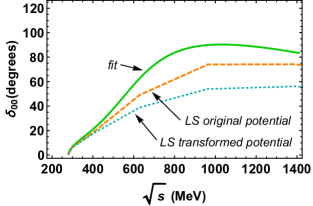
Figure 1: Comparison of results obtained using the discretized scattering equation for the reaction matrix with $N=25$ points using the prescription $K2$ for the 00 $\pi\pi$ phase-shift (see main text) and its evolved result after a uniparametric family of unitary operators according to $\xi=-i[H_{0},V]$.

III.3 Reaction matrix on the grid

The scattering problem for the reaction matrix associated with the Kadyshevsky equation for the half-off shell reaction matrix on the grid reads (the limit $\epsilon\to 0$ is already taken)

$$R_{nm}=V_{nm}+\sum_{k\neq m}^{N}V_{nk}w_{k}\frac{p_{k}^{2}}{4E_{k}^{2}}\frac{1}{2E_{m}-2E_{k}}R_{km}\ ,$$ (40)

where $R_{nm}\equiv r(p_{n},p_{m},2E_{m})$ and the restricted sum, $\sum_{k\neq m}$, implements in the momentum grid the principal value prescription. This problem can directly be solved by $N$ matrix inversions for every single energy $E_{n}$ in the grid, whence the phase-shift can be extracted using Eq. (8) evaluated on the grid points (prescription K2),

$$-\tan\delta_{l}^{\text{K2}}(p_{n})=\frac{\pi p_{n}}{8E_{n}}R_{nn}\ .$$ (41)

Our arguments, apply equally well to the discretized form of Eq.(9) as given by Eq. 40 and in Figure 1 we show for definiteness a particular case obtained by generating a uniparametric family of unitary operators according to $\xi=-i[H_{0},V]$ so that the infinitesimal change $\Delta V=[[H_{0},V],H]\Delta s$ and we integrate from $s=0$ to $s=10$ fm² (see e.g. Ref. Gomez-Rocha:2019zkz and references therein).

III.4 Scattering on the grid with observation points

Finally, let us consider the original approach of Haftel and Tabakin for Eq. (12), where in addition to the grid points, $p_{1},\dots,p_{N}$, the notion of observation point, say $k_{0}\neq p_{n}$, is introduced. The algorithm to find the phases is given by the equation

$$R(p,k_{0},2E_{0}) = V(p,k_{0})+\sum_{k=1}^{N}\frac{w_{k}p_{k}^{2}}{4E_{k}^{2}}\frac{V(p,p_{k})R(p_{k},k_{0},2E_{0})}{2E_{0}-2E_{k}}$$ (42)

$$- \sum_{k=1}^{N}\frac{w_{k}k_{0}^{2}}{4E_{0}}\frac{V(p,k_{0})R(k_{0},k_{0},2E_{0})}{k_{0}^{2}-p_{k}^{2}}$$

$$= \sum_{k=0}^{N}V(p,p_{k})R(p_{k},k_{0},2E_{0})D_{k}$$

where $E_{k}=\sqrt{p_{k}^{2}+m^{2}}$ and $E_{0}=\sqrt{k_{0}^{2}+m^{2}}$. Taking $p=p_{n}$ and $p=k_{0}$ one generates $N+1$ equations. To ease the notation we define $\rho_{n0}=R(p_{n},k_{0},2E_{0})$ and $\rho_{00}=R(k_{0},k_{0},2E_{0})$, so that the equations read

$$\rho_{n0} = V_{n0}+\sum_{k=1}^{N}D_{k}V_{nk}\rho_{k0}+D_{0}V_{n0}\rho_{n0}$$ (43)

$$\rho_{00} = V_{00}+\sum_{k=1}^{N}D_{k}V_{0k}\rho_{k0}+D_{0}V_{00}\rho_{00}$$ (44)

where

$$D_{k}=\left\{\begin{array}[]{lr}\frac{w_{k}p_{k}^{2}}{4E_{k}^{2}}\frac{1}{2E_{0}-2E_{k}},&\text{for }1\leq k\leq N\\ \frac{w_{k}k_{0}^{2}}{4E_{0}}\frac{1}{k_{0}^{2}-p_{k}^{2}},&\text{for }k=0\end{array}\right.$$ (47)

In the continuum $D_{0}$ vanishes, but on the finite grid it actually improves the accuracy. The solution is given by $R(k_{0},k_{0},2E_{0})$, similarly to Eq. (8) (prescription K3), namely

$$-\tan\delta_{l}^{\text{K3}}(k_{0})=\frac{\pi k_{0}}{8E_{0}}R_{l}(k_{0},k_{0},2E_{0})\ .$$ (48)

The question if we can check whether the calculated phase-shift, or $\rho_{00}=R(k_{0},k_{0},2E_{0})$, at the observation point $k_{0}$ is isospectral or not, i.e. under the changes $\Delta V=i[\xi,H]$ on the grid requires to distinguish two relevant cases, depending on whether the observation point is included or not in the unitary transformation.

We sketch here a perturbative proof that isospectrality does not hold. In perturbation theory, and going to the barred basis we get to second order

$$\overline{\rho}_{00} = \overline{V}_{00}+\sum_{k=1}^{N}\overline{D}_{k}\overline{V}_{0k}^{2}+\overline{D}_{0}\overline{V}_{00}^{2}+{\cal O}(V^{3})$$ (49)

so that because in any case $\Delta\overline{V}_{00}=0$ and

$$\Delta\overline{V}_{0k} = -\Delta\overline{V}_{k0}$$ (50)

$$= i\sum_{l=1}^{N}\left(\xi_{0l}\overline{H}_{lk}-\overline{H}_{0l}\xi_{lk}\right)+i(\xi_{00}\overline{H}_{0k}-\overline{H}_{00}\xi_{0k})$$

where $\overline{H}_{0l}=\overline{V}_{0l}$ and $\overline{H}_{lk}=2E_{l}\delta_{lk}+\overline{V}_{lk}$ and we have

$$\Delta\overline{\rho}_{00} = 2\sum_{k=1}^{N}\frac{1}{2E_{0}-2E_{k}}\overline{V}_{0k}\Delta\overline{V}_{k0}+{\cal O}(V^{3})$$ (51)

which is non-vanishing. Non-perturbatively we may take specific unitary transformations. While the observation points can be chosen arbitrarily, generally, we observe that close to the momentum grid points the phase-shifts are particularly unstable against unitary transformations either in the space ${\cal H}_{N}$ or ${\cal H}_{N+1}$. We have also analyzed the case of an unitary uniparametric family where infinitesimally $\Delta V=[[H_{0},V],H]\Delta s$ Gomez-Rocha:2019zkz using a grid of $N+1$ observation points $k_{n}$ nested into the grid of $N$ momentum points $p_{n}$, i.e. $k_{0}<p_{1}<k_{2}<p_{2}<\dots<p_{n}<k_{n}$ which generates a $2N+1$ dimensional space which leads to similar results.

IV Isospectral phase-shifts

The requirement of isospectrality naturally suggests to determine the phase shifts from the spectrum of the Hamiltonian, a fact noted by DeWitt DeWitt:1956be and Fukuda and Newton Fukuda:1956zz long ago based on equidistant energy or momentum grids respectively. Here we will present three different alternatives based on the Gauss-Chebyshev grid whose performance will be analyzed in the next section. On the momentum grid, the eigenvalues equation can be written as 

$$H\Psi_{n}\equiv 2E_{n}\Psi_{n}+\sum_{k}w_{k}\frac{p_{k}^{2}}{4E_{k}^{2}}V_{n,k}\Psi_{k}=\sqrt{s}\,\Psi_{n}\ ,$$ (52)

where $\Psi_{n}\equiv\langle p_{n}|\Psi\rangle$. Denoting the $N$ eigenvalues and eigenfunctions as

$$\Psi_{n,\alpha}\qquad\sqrt{s_{\alpha}}\equiv 2E_{\alpha}\ ,$$ (53)

we write the energy in the form

$$E_{\alpha}=\sqrt{P_{\alpha}^{2}+m_{\pi}^{2}}\ ,$$ (54)

where $P_{\alpha}$ is the “distorted” momentum by the interaction. As it was proposed in Fukuda:1956zz and exemplified in Arriola:2014aia ; Arriola:2016fkr the phase-shift can be identified as the momentum shift in units of the momentum resolution, namely 

$$\delta_{n}(P_{n})=-\pi\frac{P_{n}-p_{n}}{\Delta p_{n}}=-\pi\frac{\Delta P_{n}}{\Delta p_{n}}\ .$$ (55)

This prescription is a consequence of describing the scattering problem in a box and imposing the physical condition of a vanishing wave function in the wall (see Gomez-Rocha:2019xum for a reexamination). It is equivalent to a trapezoidal rule quadrature, and for a Chebyshev grid can be written as

$$\delta_{n}^{\text{MS}}(P_{n})=-\pi\frac{P_{n}-p_{n}}{w_{n}}\ ,$$ (56)

where the label MS stands for momentum-shift formula.

Another prescription is given by DeWitt DeWitt:1956be which relates the phase shifts with the energy-levels shift produced in the stationary states of a system bound in a large spherical box, when a finite-range perturbation is introduced. This is formulated in the following way

$$\delta_{n}=-\pi\frac{\Delta E_{n}}{\Delta e}\ ,$$ (57)

where $\Delta E_{n}$ is the shift from the unperturbed to the perturbed energy levels and $\Delta e$ is the separation between levels in the unperturbed system. In terms of momentum-grid points the energy-shift (ES) formula reads

$$\delta_{n}^{\text{ES}}=-\pi\frac{\sqrt{p_{n}^{2}+m^{2}}}{p_{n}w_{n}}\left(\sqrt{P_{n}^{2}+m^{2}}-\sqrt{p_{n}^{2}+m^{2}}\right)\ .$$ (58)

Note that in the ultrarelativistic case, i.e. for very small masses Eqs. (59) and (58) are equivalent. This situation holds in the $\pi\pi$ scattering case at intermediate energies.

Based on DeWitt’s argument, we have generalized the formula Eq. (58) to any momentum grid in the non-relativistic case Gomez-Rocha:2019xum , even in the case that the energy levels are not equidistant. As an example, we consider the employed momentum grid in this work, Eqs. (22)-(25). Using the analogy between the energy levels of scattering states in a box and the discretization given by a finite grid, and observing that the equidistance happens in the argument of the cosine function, we have prescribed Gomez-Rocha:2019xum the following $\phi$-shift formula based on the shift of such an angle, and write:

$$\delta_{n}^{\Phi S}=-\pi\frac{\Phi_{n}-\phi_{n}}{d\phi_{n}}=-\pi\frac{\Delta\phi_{n}}{d\phi_{n}}\ .$$ (59)

where $\phi_{n}={\pi\over N}\left(n-{1\over 2}\right)$, $d\phi_{n}={\pi\over N}$, and the “distorted” angles $\Phi_{n}$ are calculated inverting Eqs. (22)-(25) replacing $p_{n}$ by $P_{n}$.

These three prescriptions, momentum-, energy- and $\phi$-shift, have been considered in the analysis of $NN$ scattering using a nonrelativistic toy model Gomez-Rocha:2019xum . We will show here again that the $\phi$-shift method prescription is the one that best reproduces the solution in the continuum. As we will see in our numerical study, the method gives reliable predictions even for a grid with a small number of points. The generalization to any momentum grid amounts to finding the variable that is distributed equidistantly along the momentum grid.

Note that if we want the value of the phase-shift at $N$ single energy values the inversion method requires $N$ matrix inversions, whereas in the spectral shift methods the $N$ phases are obtained at once in a single diagonalization.

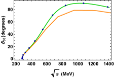
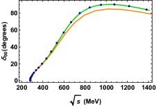
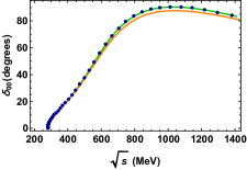
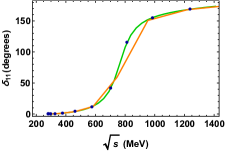
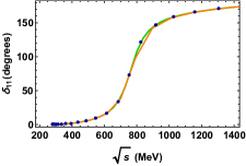
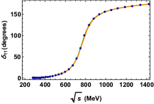
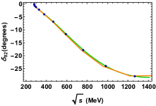
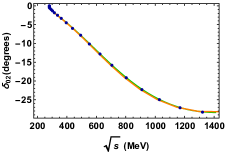
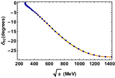
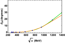
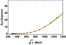
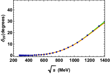
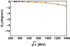
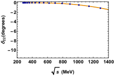
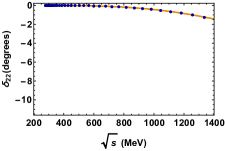
Figure 2: (Color online) Phase shifts calculated using our $\phi$-shift prescription (blue dots) compared with the numerical fit (green, smooth line) and with the result obtained from the Lippmann-Schwinger equation (step-wise, orange line). Each column corresponds to the calculation made with a grid of $N=25$, 50, and 100 points, respectively.

V Numerical results

The purpose of this numerical analysis is to study the predictive power and the accuracy of the $\phi$-shift method in the relativistic case of $\pi\pi$ scattering, in a similar way as it was done in the case of $NN$-scattering using a nonrelativistic toy model Gomez-Rocha:2019xum . For completeness and in order to compare the mass effect in the different cases, we are going to consider also several channels in $NN$ and $\pi N$ scattering to illustrate the heavy and heavy-light systems respectively. We will use here more realistic potentials than the ones used in Gomez-Rocha:2019xum .

V.1 Separable models

For definiteness, we use the form of potentials determined by the fit already carried out by H. Garcilazo and L. Mathelitsch Mathelitsch:1986ez for the lowest partial waves using separable potentials and upgrade the fitting parameters to the newest phases reported by the most recent Madrid group 2011 analysis GarciaMartin:2011cn . The most remarkable feature of these fits is the very long tail of the interaction, particularly for the $P$-wave, which reaches up to 10 GeV.

Long tails in momentum space indicate large strengths in configuration space. In fact the effect has been observed in the Marchenko approach to the inverse scattering problem Sander:1997br . The effect becomes milder when the interaction is coarse grained.

The long-tails feature is not just an artifact of the fit, as for instance the inverse scattering problem in coordinate space provides very short-distance local potentials Sander:1997br . Of course, the fact that the potential is separable, of the form

$$V_{l}(p^{\prime},p)=\eta g_{l}(p^{\prime})g_{l}(p)\ ,$$ (60)

where $\eta=\pm 1$ facilitates the solution, reducing it to a simple quadrature. Indeed, the Kadyshevsky equation, Eq. (5) is solved by the ansatz

$$T_{l}(p^{\prime},p,\sqrt{s})=g_{l}(p^{\prime})g_{l}(p)T_{l}(\sqrt{s})\ ,$$ (61)

and inserting this in Eq. (5) we get

$$\left[T_{l}(\sqrt{s})\right]^{-1}=1-\int_{0}^{\infty}dq\,\frac{q^{2}}{4E_{q}^{2}}\frac{\eta\left[g_{l}(q)\right]^{2}}{\sqrt{s}-2E_{q}}\ ,$$ (62)

yielding the final result

$$p\cot\delta_{l}(p)=-\frac{8E_{p}}{\pi V_{l}(p,p)}\left[1-\mathchoice{{\vbox{\hbox{$\textstyle-$}}\kern-4.86108pt}}{{\vbox{\hbox{$\scriptstyle-$}}\kern-3.25pt}}{{\vbox{\hbox{$\scriptscriptstyle-$}}\kern-2.29166pt}}{{\vbox{\hbox{$\scriptscriptstyle-$}}\kern-1.875pt}}\!\int_{0}^{\infty}dq\,\frac{q^{2}}{4E_{q}^{2}}\frac{V_{l}(q,q)}{\sqrt{s}-2E_{q}}\right]\ ,$$

whence the phase-shifts can directly be computed by any convenient integration method for any value of the CM energy, $\sqrt{s}$. Taking these values, we may then proceed to check the three different prescriptions, which only generate them on grid points. Form factors Eq. (60) are given in the Appendix A.

Following our preivous work Gomez-Rocha:2019xum , we consider the abbreviations $p$-shift, $E$-shift, and $\phi$-shift when refering to the momentum-shift, energy-shift and angle-shift formulas, cf. Eq. (56), (58) and (59), respectively.

V.2 Dependence on the momentum grid and comparison with the standard method

The first case we take into consideration in some detail is the $\pi\pi$-scattering. First of all, we study how our $\phi$-shift results, calculated in a finite momentum grid, differ from the exact solution in the continuum and compare our results with the procedure of solving the Lippmann-Schwinger (LS) like equation in the same momentum grid (prescription K2).

In Figure 2 we show our $\phi$-shift results (blue dots), which turn out to lie exactly on the smooth, green line that represents the exact solution. The LS calculation is represented by the orange line. Each arrow in Fig. 2 corresponds to a different channel, and each column corresponds to a different number of grid points used in the calculation, namely, $N=$25, 50, 100, respectively.

Similarly to what we observed in the non relativistic case Gomez-Rocha:2019xum , the $\phi$-shift formula provides excellent results in all cases, reproducing very accurately the exact solution, even in the case of the grid with the smallest number of points, $N=$25. While the LS method converges to the continuum as the number of points increases (the exception is the $P1$ wave, where the LS turns out to predict values very accurately in the whole interval), the $\phi$-shift results do not move away from the exact solution in any visible way in the considered grids. Recall furthermore, that only half of the points are inside the studied interval, while the other half are distributed along the long tail of the potential.

Both methods turn out to be very similar and accurate in the case of the $LI=S2$, $D0$ and $D2$ waves. This is foreseeable, since while in the first two cases the phase shifts cover a wide range of values in a short energy interval, in the last three channels, the phase shifts remain rather small ($\delta_{02},\delta_{20}<\pm 30^{o}$ and $\delta_{22}<3^{o}$) in the same energy range. Thus, perturbation theory becomes applicable and the main difference is just a higher order effect.

The $\phi$-shift method for calculating phase shifts turns out to provide outstanding results in the $\pi\pi$-scattering phase shifts. They are comparable or better than those provided by conventional approaches.

V.3 Comparison of the three different prescritpions

In this section we calculate phase shifts using the three different prescriptions presented in Section IV.

When using the $\phi$-shift, Eq. (59), or $E$-shift prescription, Eq. (58), we may represent the results as a function of the distorted momentum $P_{n}$, or as a function of the free momentum $p_{n}$. The phase shifts $\delta(P_{n})$ and $\delta(p_{n})$ will acquire the same values but will be horizontally displaced from each other by the momentum shift. This ambiguity does not arise in the $p$-shift case, since the phase shift is a function of the interacting momentum by construction.

Fig. 3 shows two lines for every $\pi\pi$-scattering channel. The upper row (in blue) shows the phase shifts calculated using the $\phi$-shift prescription, Eq. 59, while the lower row (in red) shows the phase shifts according to the energy-shift prescription, Eq. (58). The $p$-shift results are numerically almost identical in this case to the $E$-shift ones, and they are not depicted in an extra graphic. Phase shifts represented as a function of the transformed momentum $P_{n}$ are plotted using a darker line with round markers while phase shifts plotted as as function of the free momentum $p_{n}$ are given by a lighter line with square markers. All these lines are compared with the exact calculation represented by the green line without markers. In some cases, we have chosen a reduced interval, in such a way that the difference between lines is more visible.

We observe in Figure 3 that in all cases, the phase shifts represented as a function of the interacting momentum $P_{n}$ lie closer to the exact solution. This was already pointed out in the nonrelativistic case studied in Gomez-Rocha:2019xum . Observing the first and third rows (blue) in Figure 3, we see that our $\phi$-shift results totally overlap the green line which is not even visible. The $E$-shift (as well as $p$-shift) prescription given in the second and forth rows (red) yields values that lie always below those provided by the momentum-shift one. In all cases, $\phi$- and $E$-shift, the phase shifts represented as a function of the free momentum $p_{n}$ (light line with square markers) appear displaced according to the momentum shift: to the right for attractive interactions, and to the left for repulsive ones. Indeed, the $P_{n}-p_{n}$ is negative for attractive interactions and positive for repulsive ones. Since the $p$-shift formula prescribes that the phase shift is a function of the interacting momentum, and the $E$-shift formula reproduces it in this case of very light masses, we assume that taking the interacting momentum as the independent variable is the most adequate option.

It was already explained in Gomez-Rocha:2019xum , that both the $E$- and $p$-shift prescriptions are actually an approximation of the $\phi$-shift formula. Indeed, the $E$-shift formula implies an equal-distance separation of energy levels, alike the $p$-shift formula implies an equal-distance separation in momentum space. The Gauus-Chebyshev grid employed here does not satisfy those conditions. Instead, the equidistant separation occurs in the Chebyshev angle. Therefore, the adequate formula for our grid is the $\phi$-shift. Nevertheless, we have seen that still the $E$- and $p$-shift formulas turn out to be a very good approximation, since the obtained results analyzed for $N=50$ points are comparable or even better than those obtained through the standard LS equation.

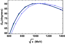
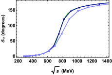
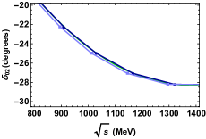
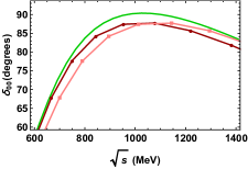
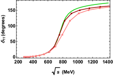
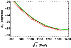
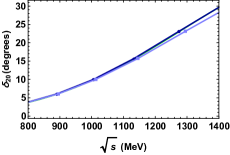
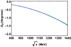
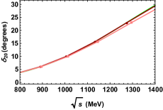
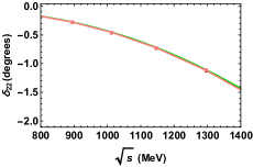
Figure 3: (Color online) Phase shifts calculated using the $\phi$-shift, $E$-shift and $p$-shift methods for every channel in $\pi\pi$-scattering and compared with the exact solution (green, smooth line). The first and third lines (in blue) show the $\phi$-shift results and the second and forth lines (in red) show the $E$- or $p$-shift results, which are equal in this case due to the relativistic pion masses. In all cases the phase shifts are represented as a function of the distorted momentum (darker line with round markers), and as a function of the free momentum (lighter line with square markers). The calculation was made with a grid of $N=50$ points.

V.4 Heavy masses and non-equal masses

Figures 4-9 show the obtained resuls for $NN$-scattering, where the form factors for separable potentials are taken from Mathelitsch:1986ez and are given in Appendix A. The phase shifts are plotted as a function of $T_{\text{Lab}}$.

The first row of each of these figures shows the $\phi$-shift result, compared with the LS results and with the exact solution for a grid of $N=25$, 50, and 100 points, respectively. The second row shows the result obtained using the $\phi$-, $p$- and $E$-shift, as labeled in the corner, for a momentum grid of $N=50$ points. In this case, the proton mass is not negligible, and hence Eqs. (56) and (58) are no longer equivalent, and the numerical difference can be appreciated (see e.g. Figure 8). In analogy to what has been done in the $\pi\pi$ analysis, we use a darker like with round markers to represent the results when using the interacting momentum as the implicit independent variable, and a lighter line with square markers when we use the free momentum as the independent variable in $T_{\text{Lab}}$. We have selected in some cases an interval where the difference between lines is more visible.

In the studied interval, $0\leq T_{\text{Lab}}\leq 300$, the phase shifts do not reach values higher than around 30 degrees, so that there are no abrupt changes in the curves and, as a consequence, the deviation from results obtained in one or other method is not significant.

Figures 10-18 show the phase shifts calculated for $\pi N$ scattering. Alike in the $NN$ case, Eqs. (56) and (58) are not equivalent due to the large mass of the proton involved. But one can hardly appreciate the difference from the numerical results due to the very small range of values that the phase shifts take in most of the channels, with the exception of the $P_{33}$ wave, which reaches from 0 to around 120 degrees.

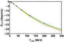
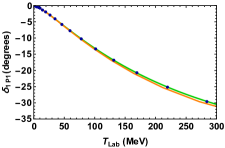
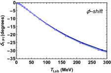
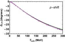
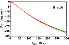
Figure 4: (Color online) $NN$-scattering phase shifts for the ${}^{1}P_{1}$ channel. Upper row: comparison of our $\phi$-shift results (blue dots) with the exact solution (green, smooth line) and the LS result (orange line) calculated in a grid of $N=25$, 50 and 100, respectively. Lower row: phase shifts calculated in a grid of $N=$50 points using the three different prescriptions as labeled in the corner. In each figure of the lower row the phase shifts are represented as a function of the distorted momentum (darker line with round markers) and as a function of the free momentum (lighter line with square markers).

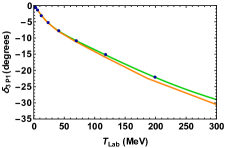
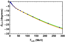
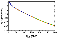
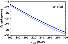
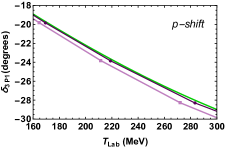
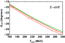
Figure 5: The same as in Figure 4 but for the ${}^{3}P_{1}$ channel.

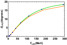
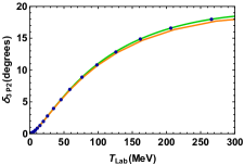
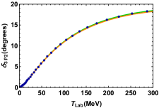
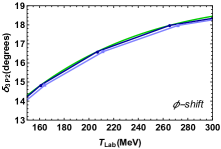
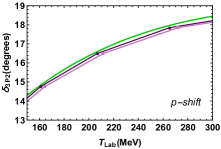
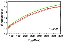
Figure 6: The same as in Figure 4 but for the ${}^{3}P_{2}$ channel.

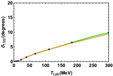
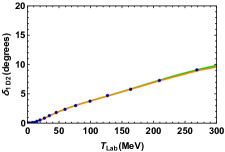
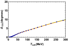
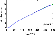
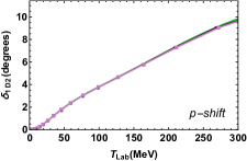
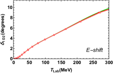
Figure 7: The same as in Figure 4 but for the ${}^{1}D_{2}$ channel.

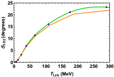
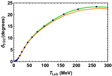
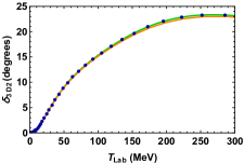
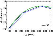
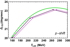
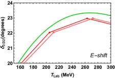
Figure 8: The same as in Figure 4 but for the ${}^{3}D_{2}$ channel.

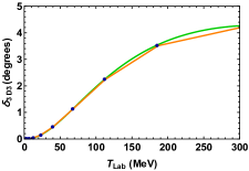
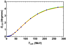
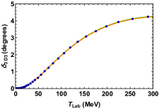
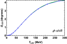
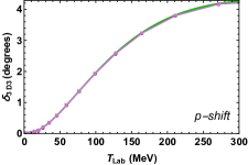
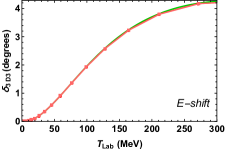
Figure 9: The same as in Figure 4 but for the ${}^{3}D_{3}$ channel.

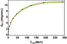
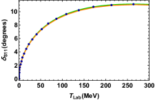
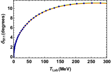
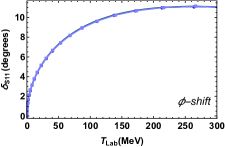
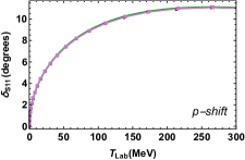
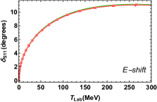
Figure 10: The same as in Figure 4 but for $\pi N$ scattering in the $S_{11}$ channel.

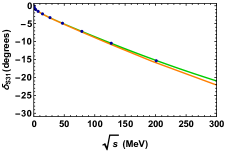
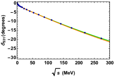
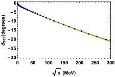
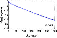
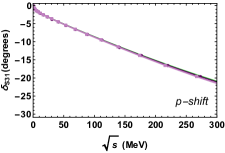
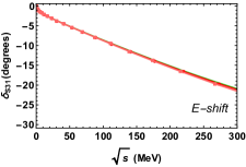
Figure 11: The same as in Figure 4 but for $\pi N$ scattering in the $S_{31}$ channel.

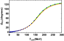
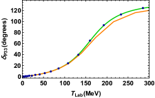
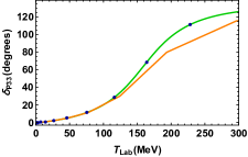
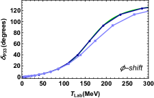
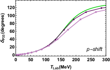
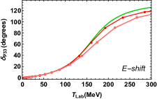
Figure 12: The same as in Figure 4 but for $\pi N$ scattering in the $P_{33}$ channel.

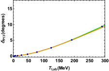
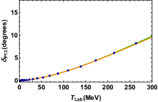
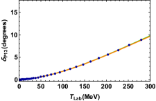
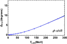
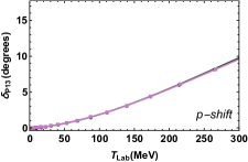
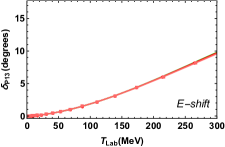
Figure 13: The same as in Figure 4 but for $\pi N$ scattering in the $P_{13}$ channel.

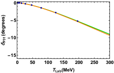
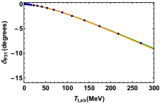
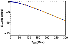
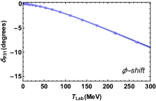
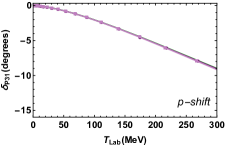
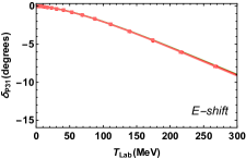
Figure 14: The same as in Figure 4 but for $\pi N$ scattering in the $P_{31}$ channel.

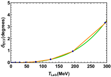
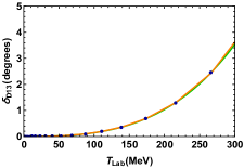
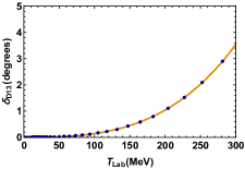
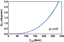
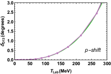
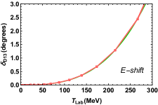
Figure 15: The same as in Figure 4 but for $\pi N$ scattering in the $D_{13}$ channel.

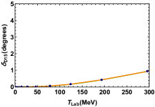
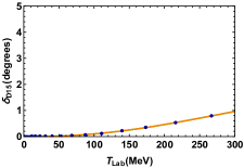
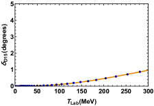
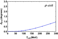
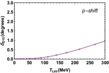
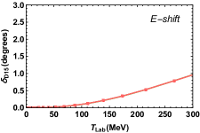
Figure 16: The same as in Figure 4 but for $\pi N$ scattering in the $D_{15}$ channel.

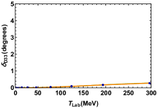
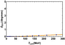
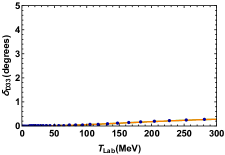
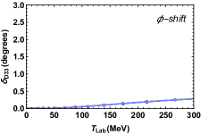
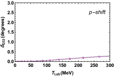
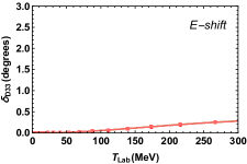
Figure 17: The same as in Figure 4 but for $\pi N$ scattering in the $D_{33}$ channel.

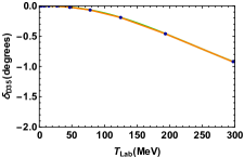
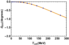
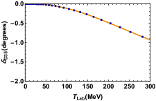
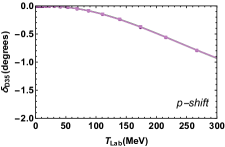
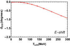
Figure 18: The same as in Figure 4 but for $\pi N$ scattering in the $D_{35}$ channel.

VI Conclusions

The analysis of hadronic interactions requires in many cases a numerical solution of the relativistic scattering problem, which from a quantum field theoretical point of view would be best formulated in terms of the 4D Bethe-Salpeter equation, but in practice one uses 3D reductions. This is most often done by placing the system in a finite momentum grid and proceeding to inverting the corresponding inhomogeneous scattering equation. In this paper we have analyzed the the Kadyshevsky equation, which allows for a corresponding relativistic interpretation of the Schrödinger equation and is fully compatible with a field theoretical Hamiltonian formulation. As we have discussed, one important feature of scattering is the freedom to carry out unitary transformations of the Hamiltonian. The discretized versions of the scattering equations violate such an invariance, and hence the computed phase-shifts are not isospectral. On the other hand, the eigenvalues of the Hamiltonian are by definition invariant, and hence it makes sense to determine the phase-shifts directly from the eigenvalues, for which several schemes have already been presented.

We have studied the predictive power of the momentum-shift and energy-shift prescriptions for calculating phase shifts. We have generalized to the relativistic case a new prescription based on an argument that holds for any momentum grid. The new prescription requires to find the variable that holds an equidistant space between points along the momentum grid. The chosen grid in this work is a Gauss-Chebyshev quadrature and the equal spacing occurs in the Chebyshev angle $\phi={{\pi\over N}(n-1/2)}$. As it turns out, this prescription yields exceptionally good results, even in the case of a grid with a relatively small number of points.

Besides providing accurate isospectral phases even in rather coarse momentum grids, our $\phi$-shift formula is computationally cheaper than any conventional solution based on the matrix inversion of the inhomogeneous scattering equation. Indeed, if we want to compute $N$ energy values of the phase-shift with a grid of $N$ points we have a computational complexity of $N\times{\cal O}(N^{3})$ because $N$-inversions are needed, whereas with the digonalization method we have at once all phase-shifts with ${\cal O}(N^{3})$ cost trefethen1997numerical . However, this happens at a price: while in our case the phases are computed at the interacting momenta, in the conventional solution the momenta are arbitrary.

All these findings are of special relevance for calculations that use a Hamiltonian framework. Indeed, many scattering studies are carried out within Lagrangian approaches, while the study of phase shifts in the context of a Hamiltonian formalism is rather sparse. It turns out, however that the Hamiltonian formalism is very convenient or even necessary for certain purposes addressing renormalization issues Gomez-Rocha:2019zkz .

The Kadyshevsky equation is very convenient in order to consider the three-body interaction problem. It is possible to couple the two-body interaction force into the three-body equation, in such a way that, for instance, a controlled knowledge of the $\pi\pi$-interaction, may lead to a precise description of $3\pi$ resonances, such as the $\omega$ or the $A_{1}$ ones. A method with such a predictive power like the one we have presented in this work, opens the possibility of making accurate predictions for such states with a rather manageable computational cost.

Appendix A From factors. Model potentials

The form factors $g_{LI}$, with $L$ being the angular momentum and $I$ the isospin, in the case of $\pi\pi$ interaction are given by

$$g_{00}(p) = \frac{617.865p^{2}}{\left(p^{2}+99.3951\right)^{2}}+\frac{423.64}{p^{2}+1034.75}\ ,$$ (64)

$$g_{11}(p) = p\left(\frac{132.237}{p^{2}+900.462}-\frac{5.11596}{p^{2}+21.9744}\right)\ ,$$ (65)

$$g_{02}(p) = \frac{3.65p^{2}}{\left(p^{2}+3.9601\right)^{2}}+\frac{175.7}{p^{2}+357.21}\ ,$$ (66)

$$g_{20}(p) = \frac{284.863p^{2}}{\left(p^{2}+53.6235\right)^{2}}\ ,$$ (67)

$$g_{22}(p) = \frac{289.289p^{2}}{\left(p^{2}+101.039\right)^{2}}\ ,$$ (68)

where all the potentials are attractive, i.e. the parameter $\eta=1$ in Eq. (60), except the 02 and the 22 that are repulsive, i.e $\eta=-1$.

For $NN$ scattering we have for every ${}^{2S+1}L_{J}$

$$g_{{}^{1}P_{1}}(p) = p\left[\frac{96.6852p^{2}}{\left(p^{2}+8.72978\right)^{3}}+\frac{104.81}{\left(p^{2}+6.17934\right)^{2}}\right]$$ (69)

$$g_{{}^{3}P_{1}}(p) = p\left[\frac{139.976p^{2}}{\left(p^{2}+4.3655\right)^{3}}+\frac{4.39386}{\left(p^{2}+0.877575\right)^{2}}\right]$$ (70)

$$g_{{}^{3}P_{2}}(p) = p\left[\frac{158.854p^{2}}{\left(p^{2}+8.16363\right)^{3}}+\frac{15.1423}{\left(p^{2}+2.91507\right)^{2}}\right]$$ (71)

$$g_{{}^{1}D_{2}}(p) = p^{2}\left[\frac{674.983}{\left(p^{2}+6.37134\right)^{3}}-\frac{179.268p^{2}}{\left(p^{2}+2.74016\right)^{4}}\right]$$ (72)

$$g_{{}^{3}D_{2}}(p) = p^{2}\left[\frac{513.691}{\left(p^{2}+4.44559\right)^{3}}-\frac{156.742p^{2}}{\left(p^{2}+2.06874\right)^{4}}\right]\$$ (73)

$$g_{{}^{3}D_{3}}(p) = p^{2}\left[\frac{357.477}{\left(p^{2}+6.99909\right)^{3}}-\frac{111.479p^{2}}{\left(p^{2}+4.26756\right)^{4}}\right]$$ (74)

and

$$\eta_{{}^{1}P_{1}} = \eta_{{}^{3}P_{1}}=1\ ,$$ (75)

$$\eta_{{}^{3}P_{2}} = \eta_{{}^{1}D_{2}}\,=\,\eta_{{}^{3}D_{2}}\,=\,\eta_{{}^{3}D_{3}}\,=\,-1\ .$$ (76)

Finally, the form factors for $\pi N$ scattering are, for every $L_{2S\,2I}$ channel

$$g_{S_{11}}(p) = \frac{14.6454}{p^{2}+12.2543}\ ,$$ (77)

$$g_{S_{31}}(p) = \frac{95.4252}{p^{2}+30.9159}-\frac{3.13741}{p^{2}+1.83667}\ ,$$ (78)

$$g_{P_{33}}(p) = p\left(\frac{36.8052}{p^{2}+102.726}+\frac{0.0867424}{p^{2}+0.226963}\right)\,,$$ (79)

$$g_{P_{13}}(p) = p\left(\frac{10.4023}{p^{2}+15.7088}-\frac{2.31101}{p^{2}+31.1786}\right)\,,$$ (80)

$$g_{P_{31}}(p) = \frac{13.079p}{p^{2}+12.222}\ ,$$ (81)

$$g_{D_{13}}(p) = \frac{364.057p^{2}}{\left(p^{2}+49.925\right)^{2}}\ ,$$ (82)

$$g_{D_{15}}(p) = \frac{10.8919p^{2}}{\left(p^{2}+6.79962\right)^{2}}\ ,$$ (83)

$$g_{D_{33}}(p) = \frac{2.18078p^{2}}{\left(p^{2}+3.20603\right)^{2}}\ ,$$ (84)

$$g_{D_{35}}(p) = \frac{7.52545p^{2}}{\left(p^{2}+5.20257\right)^{2}}\ ,$$ (85)

and

$$\eta_{S_{31}} = \eta_{P_{31}}\,=\,\eta_{D_{35}}\,=\,1\ ,$$ (86)

$$\eta_{S_{11}} = \eta_{P_{13}}\,=\,\eta_{D_{13}}\,=\,\eta_{D_{15}}\,=\,\eta_{D_{33}}\,=\,-1\ .$$ (87)

In all cases the parameters have units of fm^-1 or fm^-2 as corresponds in such a way that the form factors are dimensionless.

References

- (1) E.E. Salpeter and H.A. Bethe, Phys. Rev. 84 (1951) 1232.
- (2) N. Nakanishi, Prog. Theor. Phys. Suppl. 43 (1969) 1.
- (3) J.S.R. Chisholm, Nucl. Phys. 26 (1961) 469.
- (4) S. Kamefuchi, L. O’Raifeartaigh and A. Salam, Nucl. Phys. 28 (1961) 529.
- (5) J. Nieves and E. Ruiz Arriola, Nucl. Phys. A679 (2000) 57, hep-ph/9907469.
- (6) M.J. Levine, J. Wright and J.A. Tjon, Phys. Rev. 154 (1967) 1433.
- (7) J. Carbonell and V.A. Karmanov, Phys. Lett. B727 (2013) 319, 1310.4091.
- (8) J. Carbonell and V.A. Karmanov, Phys. Rev. D90 (2014) 056002, 1408.3761.
- (9) B.A. Lippmann and J. Schwinger, Phys. Rev. 79 (1950) 469.
- (10) R.H. Landau, Quantum mechanics. Vol. 2: A second course in quantum theory (, 1990).
- (11) F. Gross, Relativistic quantum mechanics and field theory (, 1993).
- (12) A.A. Logunov and A.N. Tavkhelidze, Nuovo Cim. 29 (1963) 380.
- (13) R. Blankenbecler and R. Sugar, Phys. Rev. 142 (1966) 1051.
- (14) V.G. Kadyshevsky, Nucl. Phys. B6 (1968) 125.
- (15) F. Gross, Phys. Rev. 186 (1969) 1448.
- (16) F. Gross, Phys. Rev. C26 (1982) 2203.
- (17) M.I. Haftel and F. Tabakin, Nucl. Phys. A158 (1970) 1.
- (18) N. Fukuda and R.G. Newton, Phys. Rev. 103 (1956) 1558.
- (19) B.S. DeWitt, Phys. Rev. 103 (1956) 1565.
- (20) E.J. Heller and H.A. Yamani, Phys. Rev. A9 (1974) 1201.
- (21) A. Deloff, Annals Phys. 322 (2007) 1373, quant-ph/0606100.
- (22) W.P. Reinhardt, D.W. Oxtoby and T.N. Rescigno, Phys. Rev. Lett. 28 (1972) 401.
- (23) J. Muga and R. Levine, Physica Scripta 40 (1989) 129.
- (24) H. Ekstein, Phys. Rev. 117 (1960) 1590.
- (25) J.E. Monahan, C.M. Shakin and R.M. Thaler, Phys. Rev. C4 (1971) 43.
- (26) W.N. Polyzou, Phys. Rev. C82 (2010) 014002, 1001.4523.
- (27) E. Ruiz Arriola, S. Szpigel and V.S. Timóteo, Phys. Lett. B735 (2014) 149.
- (28) E. Ruiz Arriola, S. Szpigel and V.S. Timóteo, Annals Phys. 371 (2016) 398, 1601.02360.
- (29) A.D. Alhaidari et al., The J-matrix method (Springer, 2008).
- (30) M. Gómez-Rocha and E. Ruiz Arriola, (2019), 1910.10560.
- (31) R.J. Yaes, Phys. Rev. D3 (1971) 3086.
- (32) J. Frohlich, K. Schwarz and H.F.K. Zingl, Phys. Rev. C27 (1983) 265.
- (33) V.M. Vinogradov, Teor. Mat. Fiz. 8 (1971) 343.
- (34) M. Polivanov and S. Khoruzhii, SOVIET PHYSICS JETP 19 (1964).
- (35) N.B. Skachkov, Teor. Mat. Fiz. 5 (1970) 57.
- (36) R.J. Yaes, Prog. Theor. Phys. 50 (1973) 945.
- (37) H. Garcilazo and L. Mathelitsch, Phys. Rev. C28 (1983) 1272.
- (38) L. Mathelitsch and H. Garcilazo, Phys. Rev. C32 (1985) 1635.
- (39) E. Ruiz Arriola, S. Szpigel and V.S. Timoteo, (2014), 1404.4940.
- (40) M. Gómez-Rocha and E. Ruiz Arriola, 15th International Conference on Meson-Nucleon Physics and the Structure of the Nucleon (MENU 2019) Pittsburgh, Pennsylvania, USA, June 2-7, 2019, 2019, 1909.01715.
- (41) R. Garcia-Martin et al., Phys. Rev. D83 (2011) 074004, 1102.2183.
- (42) M. Sander and H.V. von Geramb, Phys. Rev. C56 (1997) 1218, nucl-th/9703031.
- (43) L.N. Trefethen and D. Bau IIINumerical linear algebra Vol. 50 (Siam, 1997).