On the behaviour of large empirical autocovariance matrices between the past and the future.
Abstract The asymptotic behaviour of the distribution of the squared singular values of the sample autocovariance matrix between the past and the future of a high-dimensional complex Gaussian uncorrelated sequence is studied. Using Gaussian tools, it is established the distribution behaves as a deterministic probability measure
whose support is characterized. It is also established that the singular values to the square are almost surely located in a neighbourhood of .
1 Introduction.
1.1 The addressed problem and the results.
In this paper, we consider a sequence of integer , and positive definite hermitian matrices . For each , we define an independent identically distributed sequence (depending on ) of zero mean complex Gaussian –dimensional random vectors such that where the components of the –dimensional vector are complex Gaussian standard i.i.d. random variables (i.e. their real and imaginary parts are i.i.d. and distributed). If is a fixed integer, we consider the 2 block-Hankel matrices and defined by
| (1.1) |
and
| (1.2) |
and study the behaviour of the empirical eigenvalue distribution of the matrix in the asymptotic regime where and converge towards in such a way that
| (1.3) |
Using Gaussian tools, we evaluate the asymptotic behaviour of the resolvent , and establish that the sequence has the same almost sure asymptotic behaviour than a sequence of deterministic probability measures. In the following, will be referred to as the deterministic equivalent of . We evaluate the Stieltjes transform of , characterize its support, study the properties of its density, and eventually establish that almost surely, for large enough, all the eigenvalues of are located in a neighbourhood of the support of .
1.2 Motivation
Matrix represents the traditional empirical estimate of the autocovariance matrix between the past and the future of defined as
This matrix plays a key role in statistical inference problems related to multivariate time series with rational spectrum. In order to explain this, we consider a –dimensional multivariate time series generated as
| (1.4) |
where is as above a Gaussian ”noise” term such that for some unknown positive definite matrix , and where is a ”useful” non observable Gaussian signal with rational spectrum. can thus be represented as
| (1.5) |
where is a –dimensional white noise sequence (), is a deterministic matrix whose spectral radius is strictly less than 1, and where are deterministic matrices. The -dimensional Markovian sequence is called the state-space sequence associated to (1.5). The state space representation (1.5) is said to be minimal if the dimension of the state space sequence is minimal. Given the autocovariance sequence of (i.e. for each ), the so-called stochastic realization problem of consists in characterizing all the minimal state space representations (1.5) of , or equivalently in identifying all the minimum Mac-Millan degree 111The Mac-Millan degree of a rational matrix-valued function is defined as the minimal dimension of the matrices for which can be represented as matrix-valued function such that and
| (1.6) |
for each . Such a function is called a minimal degree causal spectral factorization of . We refer the reader to [24] or [36] for more details.
The identification of and of matrices and is based on the observation that the autocovariance sequence of can be represented as
| (1.7) |
for each , where the 3 matrices are unique up to similarity transforms, thus showing that the matrices and associated to a minimal realization are uniquely defined (up to a similarity). Moreover, the autocovariance matrix between the past and the future of can be written as
| (1.8) |
where matrix is the ”observability” matrix
| (1.9) |
and matrix is the ”controllability” matrix
| (1.10) |
For each , the rank of remains equal to , and each minimal rank factorization of
can be written as (1.8) for some particular triple . In particular, if
is the singular value decomposition of , matrix
coincides with the observability matrix of a pair . and are immediately
obtained from the knowledge of the structured matrix . This discussion shows that the evaluation of , and from
the autocovariance sequence of is an easy problem. We mention that, while and are essentially unique, there exist in general more than
1 pair for which (1.5) holds because the minimal degree spectral factorization problem (1.6) has
more than 1 solution. We refer the reader to [24] or [36].
We notice that as in (1.4) is an uncorrelated sequence, it holds that coincides with for each . Therefore, and matrices and can still be identified from the autocovariance sequence of the noisy version of . In practice, however, the exact autocovariance sequence is in general unknown, and it is necessary to estimate and from the sole knowledge of samples . For this, is first estimated as the number of significant singular values of the empirical estimate of the true matrix defined by
where and are defined in the same way than and . If and are the largest singular values and corresponding left singular vectors of matrix , and if is the diagonal matrix with diagonal entries , matrix is an estimator of an observability matrix . has not necessarily the structure of an observability matrix, but it is easy to estimate by finding the minimum of the quadratic fuction
where the operator ”down” (resp. ”up”) suppresses the last (resp. the first) rows from matrix
. This approach provides a consistent estimate of when while , and are fixed
parameters. We refer the reader to [10] for a detailed analysis of this statistical inference scheme.
If is large and that the sample size cannot be arbitrarily larger than , the ratio may not be small enough to make reliable
the above statistical analysis. It is thus relevant to study the behaviour of the above estimators in asymptotic regimes where and both converge towards in such a way that converges towards a non zero constant. In this context, the truncated singular value decomposition of does not provide a consistent estimate of an observability matrix , and it appears relevant to study the largest singular values and corresponding singular vectors of when and both converge towards , and to precise how they are related to an observability matrix .
Without formulating specific assumptions on , this problem seems very complicated. In the past, a number of works addressed high-dimensional inference schemes based on the eigenvalues and eigenvectors of the empirical covariance matrix of the observation (see e.g. [30], [28], [31], [17], [37], [38], [11], [35]) when the useful signal lives in a low-dimensional deterministic subspace. Using results related to spiked large random matrix models (see e.g. [3] [4], [33]), based on perturbation technics, a number of important statistical problems could be addressed using large random matrix theory technics. Our ambition is to follow the same kind of approach to address the estimation problem of when satisfies some low rank assumptions. The first part of this program is to study the asymptotic behaviour of the singular values of the empirical autocovariance matrix in the absence of signal . As the singular values of are the square roots of the eigenvalues of , this is precisely the topic of the present paper. Using the obtained results, it should be possible to use a perturbation approach in order to evaluate the behaviour of the largest singular values and corresponding left singular vectors in the presence of a useful signal, and to deduce from this some improved performance scheme for estimating .
1.3 On the literature.
The large sample behaviour of high-dimensional autocovariance matrices was comparatively less studied than the
high-dimensional covariance matrices. We first mention [21] which studied the asymptotic behaviour of
the eigenvalue distribution of the hermitian matrix where is defined as
where represents
a dimensional non Gaussian i.i.d. sequence, the components of each vector being morever i.i.d. In particular,
. It is proved that the empirical eigenvalue distribution of converges towards a
limit distribution independent from . Using finite rank perturbation technics of the resolvent of the matrix under consideration, the Stieltjes transform of this distribution was shown
to satisfy a polynomial degree 3 equation. Solving this equation led to an explicit
expression of the probability density of the limit distribution. [25] extended these
results to the case where is a non Gaussian linear process
where is i.i.d., and where matrices are simultaneously diagonalizable. The limit
eigenvalue distribution was characterized through its Stieltjes transform that is obtained by integration of a certain kernel, itself solution of an integral equation. The proof was based on the observation that in the Gaussian case,
the correlated vectors can be replaced by independent ones using a classical
frequency domain decorrelation procedure. The results were generalized in the non Gaussian case using the generalized Lindeberg principle. We also mention [1] (see also the book
[2]) where the existence of a limit distribution of any symmetric polynomial
of for some finite set was proved using the moment method when is a linear non Gaussian process. [22] studied the asymptotic behaviour of
matrix when represents
a dimensional non Gaussian i.i.d. sequence, the components of each vector being morever i.i.d.
Using finite rank perturbation technics, it was shown that the empirical eigenvalue distribution converges
towards a limit distribution whose Stieltjes transform is solution of a degree 3 polynomial equation. As
in [21], this allowed to obtain the expression of the corresponding probability
density function. Using combinatorial technics, [22] also established that almost surely,
for large enough dimensions, all the eigenvalues of are located
in a neighbourhood of the support of the limit eigenvalue distribution. We finally mention that [23] used the results in [22] in order to study the largest eigenvalues and corresponding eigenvectors of when the observation contains a certain spiked useful signal that is more specific than the signals
signals that motivated the present paper.
We now compare the results of the present paper with the content of the above previous works. We first study
a matrix that is more general than . While we do not consider linear processes
here, we do not assume that the covariance matrix of the i.i.d. sequence is reduced
to as in [22]. This in particular implies that the Stieltjes transform of the
deterministic equivalent of cannot be evaluated in closed from. Therefore, a dedicated
analysis of the support and of the properties of is provided here. We also mention
that in contrast with the above papers, we characterize the asymptotic behaviour of the resolvent of
matrix while the mentionned previous works only studied
the normalized trace of the resolvent of the matrices under consideration. Studying the full resolvent
matrix is necessary to address the case where a useful spiked signal is added to the noise .
We notice that the above papers addressed the non Gaussian case while we consider the case where
is a complex Gaussian i.i.d. sequence. This situation is of course simpler in that various Gaussian
tools are available, but appears to be
relevant because in the context of the present paper, is indeed supposed to represent some additive
noise, which, in a number of contexts, is Gaussian. In any case, it should be possible to
extend the present results to the non Gaussian case by using the Lindeberg principle or some
interpolation scheme.
We finally mention that some of the results of this paper may be obtained by adapting general recent results devoted to the study of the spectrum of hermitian polynomials of GUE matrices and deterministic matrices (see [5] and [27]). If we denote by the matrix , then can be written as where the entries of are i.i.d. complex Gaussian standard variables. Each block () of is clearly a polynomial of and various and deterministic matrices. Assume that . In order to be back to a polynomial of GUE matrices, it possible to consider the matrix whose blocks are defined by
It is clear that apart , the eigenvalues of coincide with those of . If is any matrix with i.i.d. complex Gaussian standard entries whose first rows coincide with , then, it is easily seen that each block of coincides with a hermitian polynomial of and deterministic matrices such as
Expressing as the sum of its hermitian and anti-hermitian parts, we are back to study the behaviour of the eigenvalues of a matrix whose blocks are hermitian polynomials of 2 independent GUE matrices and of deterministics matrices. Extending Proposition 2.2 and Theorem 1.1 in [5] to block matrices (as in Corollary 2.3 in [27]) would lead to the conclusion that has a deterministic equivalent and that the eigenvalues of are located in the neighbourhood of the support of . While this last consequence would avoid the use of the specific approach used in section 9 of the present paper, the existence of is not a sufficient information. should of course be characterized through its Stieltjes transform, and we believe that the adaptation of Proposition 2.2 and Theorem 1.1 in [5] is not the most efficient approach.
1.4 Overview of the paper.
As the entries of matrices and are correlated, approaches based on finite rank perturbation of the resolvent of matrix , usually used when independence assumptions hold, are not the most efficient in our context. We rather propose to use Gaussian tools, i.e. integration by parts formula in conjunction with the Poincaré-Nash inequality (see e.g. [32]), because they are robust to correlation of the matrix entries. Moreover, as the entries of are biquadratic functions of , we rather use the well-known linearization trick that consists in studying the resolvent of the hermitized version
of matrix . As is well known, the first diagonal block of
coincides with . Therefore, we characterize the asymptotic behaviour of
, and deduce from this the results concerning . The hermitized version
is this time a quadratic function of , and the Gaussian calculus that is needed in order
to study appears much simpler than if was evaluated directly.
In section 3, we evaluate the variance of useful functionals for using the Poincaré-Nash inequality. In section 4, we establish some useful lemmas related to certain Stieltjes transforms. In section 5, we use the integration by parts formula to establish that behaves as where is defined by
where is defined by where represents the first diagonal block of . We deduce from this that
where , , and where is an error term such that
for each , where and are 2 polynomials whose degrees and coefficients do not depend on . Using this, we prove in section 7 that for each ,
where is any deterministic sequence of matrices such that , and where is defined by
being the unique solution of the equation
| (1.11) |
such that and belong to when . and are shown to coincide with the Stieltjes transforms of a scalar measure and of a positive matrix valued measure respectively, and it is proved that is a probability measure such that weakly almost surely. is referred to as the deterministic equivalent of . In section 8, we study the properties and the support of , or equivalently of because the 2 measures are absolutely continuous one with respect to each other. For this, we study the behaviour of when converges towards the real axis. For each , the limit of when converges towards exists and is finite. If , we deduce from this that is absolutely continuous w.r.t. the Lebesgue measure. The corresponding density is real analytic on , and converges towards when . If , it holds that while if . If , contains a Dirac mass at with weight and an absolutely continuous component. In order to analyse the support of and , we establish that the function defined by
is solution of the equation for each where is the function defined by
Moreover, if we define for by the limit of when , the equality is also valid on . We establish that if is outside the support of , then, it holds that
This property allows to prove that apart when , the support of is a union of intervals whose end points are the extrema of whose arguments verify . A sufficient condition on the eigenvalues of ensuring that the support of is reduced to a single interval is formulated. Using the
Haagerup-Thornbjornsen approach ([15]), it is moreover proved in section 9 that for each large enough, all the eigenvalues of
lie in a neighbourhood the support of the deterministic equivalent . The above results do not imply that converges towards a limit distribution. In order to obtain this kind of result, some extra assumptions have to be
formulated, such as the existence of a limit empirical eigenvalue distribution for when
. If the relevant conditions are met, , and therefore
, will converge towards a limit distribution whose Stieltjes transform can be
obtained by replacing in the above results the empirical eigenvalue of by its limit.
We do not present the corresponding results here because we believe that results that
characterize the behaviour of for each large enough are more informative
than the convergence towards a limit.
In section 10, we finally indicate that the use of free probability tools is an alternative approach to characterize the asymptotic behaviour of . The results of section 10 are based on the following observations:
-
•
Up to the zero eigenvalue, the eigenvalues of coincide with the eigenvalues of
-
•
While the matrices and do not satisfy the conditions of the usual asymptotic freeness results, it turns out that they are almost surely asymptotically free. Therefore, the eigenvalue distribution of converges towards the free multiplicative convolution product of the limit distributions of and . These two distributions appear to coincide both with the limit distribution of the well known random matrix model where is a complex Gaussian random matrix with standard i.i.d. entries.
The asymptotic freeness of and appear to be a consequence of Lemma 6 in [13]. While this approach seems to be simpler than the use of the Gaussian tools proposed in the present paper, we mention that the above free probability theory arguments do not allow to study the asymptotic behaviour of the resolvent of . We recall that in order to evaluate the largest eigenvalues and corresponding eigenvectors of in the presence of a useful signal, the asymptotic behaviour of the full resolvent in the absence of signal has to be available.
2 Some notations, assumptions, and useful results.
In the following, it is assumed that is a fixed parameter, and that and converge towards in such a way that
| (2.1) |
This regime will be referred to as in the following. In the regime (2.1), should be interpreted as an integer depending on . The various matrices we have introduced above thus depend on and will be denoted . In order to simplify the notations, the dependency w.r.t. will sometimes be omitted.
We recall that the resolvent of is defined by
| (2.2) |
As the direct study of is not obvious, we rather introduce the resolvent of the block matrix
It is well known that can be expressed as
| (2.3) |
where is the resolvent of matrix . As shown below, it is rather easy to
evaluate the asymptotic behaviour of using the Poincaré-Nash inequality and the integration
by part formula (see Propositions 2 and 1 below). Formula (2.3) will then provide all the necessary information on
.
In the following, every matrix will be written as
where the 4 matrices are . Sometimes, the blocks will be denoted , ,
….
We denote by the matrix defined by
| (2.4) |
Its elements satisfy
where represents the element which lies on the -th line and -th column for , and . Similarly, , where and , represents the entry of . For each , and are the column of matrices and respectively. For each and , represents the vector of the canonical basis of with 1 at the index and zeros elsewhere. In order to simplify the notations, we mention that if , vector may also represents the vector of the canonical basis of with 1 at the index and zeros elsewhere. Vector with represents the –th vector of the canonical basis of . Also for any integer , is the ”shift” matrix defined by
| (2.5) |
In order to short the
notations, matrix is denoted , although is of course not invertible.
By a nice constant, we mean a positive deterministic constant which does not depend on the dimensions and nor of the complex variable . In the following, will represent a generic nice constant whose value may
change from one line to the other. A nice polynomial is a polynomial whose degree and coefficients
are nice constants. Finally, we will say that function if belongs to a domain and there exist two nice polynomials and such that for each . If , we will just write
without mentioning the domain. We notice that
if , and , are nice polynomials, then , from which we conclude that if functions and are then also .
The sequence of covariance matrices of –dimensional vectors is supposed to verify
| (2.6) |
for each , where and are 2 nice constants. represent the eigenvalues of arranged in the decreasing order and denote the corresponding eigenvectors. Hypothesis
(2.6) is obviously equivalent to and for
each .
The eigenvalues and eigenvectors of matrix are denoted
and respectively.
represents the set of all real valued compactly supported functions defined on .
If is a random variable, we denote by the zero mean random variable defined by
| (2.7) |
We finally recall the 2 Gaussian tools that will be used in the sequel in order to evaluate the asymptotic behaviour of and .
Proposition 1
(Integration by parts formula.) Let be a complex Gaussian random vector such that , and . If is a complex function polynomially bounded together with its derivatives, then
| (2.8) |
Proposition 2
(Poincaré-Nash inequality.) Let be a complex Gaussian random vector such that , and . If is a complex function polynomially bounded together with its derivatives, then, noting and
| (2.9) |
3 Use of the Poincaré-Nash inequality.
In this paragraph, we control the variance of various functionals of using the Poincaré-Nash inequality. For this, it appears useful to evaluate the moments of . The following result holds.
Lemma 1
For any , it holds that
Proof. We first remark that it is possible to be back to the case where matrix . Due to the Gaussianity of the i.i.d. vectors , it exists i.i.d. distributed vectors such that verifying . From this, we obtain immediately that the block Hankel matrix built from satisfies
| (3.1) |
As the spectral norm of is assumed uniformly bounded when increases, the statement of the lemma is equivalent to . It is shown in [26] that the empirical eigenvalue distribution of converges towards the Marcenko-Pastur distribution, and that its smallest non zero eigenvalue and its largest eigenvalue (which coincides with ) converge almost surely towards and respectively. We express as
where is a nice constant. As , it is sufficient to prove that is less than any power of . We introduce a smooth function defined on by
and elsewhere. Then, it holds that
for any . Lemma 1 thus appears as an immediate consequence of the following lemma.
Lemma 2
For each smooth function such that if and constant on , it holds that , .
Proof. We prove the Lemma by induction. We first consider the case . For more convenience we will write instead of in the course of the proof. Here and below we take sum for all possible values of indexes, if not specified. From (2.9) we have
| (3.2) |
We only evaluate the first term, denoted by , of the right handside of (3), because the second one can be addressed similarly. For this, we first remark that
Plugging this into (3) we obtain
Denoting , it is easy to verify that can be written as
| (3.3) |
where we recall that matrix is defined by (2.5). For each matrices and , the Schwartz inequality and the inequality between arithmetic and geometric means lead to
Therefore, since and
| (3.4) |
By taking here , we obtain from (3) and (3.3)
| (3.5) |
Consider the function . It is clear that is a compactly supported smooth function. Therefore (see e.g. [26]), it holds that
where is the measure associated to Marcenko-Pastur distribution with parameters (1, ) and where represents the support of . It is clear that for large enough, the support of and do not intersect, so that . Therefore, we obtain that
This and (3.5) lead to the conclusion that . To finalize the case , we express as . [26, Lemma 10.1] implies that , which completes the proof for .
Now we suppose that for any we have and are about to prove that it holds for . As in the previous case we write
| (3.6) |
To evaluate the second term of the r.h.s. of (3.6), we use the Schwartz inequality and the induction assumption
| (3.7) |
We follows the same steps as in the case to study the first term of the r.h.s. of (3.6). Using again the Poincaré-Nash inequality, we obtain that
| (3.8) |
Using Holder’s inequality, we obtain
| (3.9) |
The properties of function imply that it satisfies the induction hypothesis and that it verifies (3.7), i.e. . Plugging this into (3.9), we get that
| (3.10) |
From this, (3.7) and (3.6), we immediately obtain
| (3.11) |
We denote by the term . Then, (3.11) implies that
This inequality leads to the conclusion that sequence is bounded, or equivalently that
as expected. This completes the proof of Lemmas 2
and 1.
We now evaluate the variance of useful functionals of the resolvent .
Lemma 3
Let , be sequences of deterministic matrices and a sequence of deterministic matrices such that , and consider sequences of deterministic –dimensional vectors , such that for . Then, for each , it holds that
| (3.12) | ||||
| (3.13) | ||||
| (3.14) |
where can be written as for some nice polynomials and .
Proof. We first prove (3.12) and denote by the term . The Poincare-Nash inequality leads to
We just evaluate the first term of r.h.s., denoted by . For this, we need the expression of the derivative of with respect to the complex conjugates of the entries of . We denote by and as matrices defined by and . Then, after some algebra, we obtain that
| (3.15) |
From this, we deduce immediately that
Using that , we obtain that is given by
We put and remark that and that . Therefore, can be written as
| (3.16) |
Each term inside the sum over can be written as , where the expression of matrix is omitted. As is bounded by the nice constant (see (2.6)), (3.4) and (3) lead to the conclusion that we just need to evaluate . Using the Schwartz inequality, we obtain immediately that
| (3.17) | ||||
Since and , we get that
Lemma 1 thus implies that
for some nice polynomial . The term can be handled similarly. Therefore, (3) leads to . This establishes (3.12).
To prove (3.13) one can also use Poincaré-Nash inequality for . After some calculations, we get that the variance of is upperbounded by a term given by
| (3.18) |
where is some nice constant, and where and are defined by
| (3.19) | |||||
| (3.20) |
Using Lemma 1 as well as the inequality , we obtain
immediately (3.13).
In the following, we also need to evaluate the variance of more specific terms. The following result appears to be a consequence of Lemma 3 and of the particular structure (2.3) of matrix .
Corollary 1
Let be a sequence of deterministic matrices such that , and a sequence of deterministic matrices satisfying . Then, if , the following evaluations hold:
| (3.21) |
where and belong to ;
| (3.22) |
where still belong to , but verify and .
Proof. We first prove (3.21), and first consider the case where . We define the matrix by for , and remark that coincides with . We follow the proof of (3.12), and evaluate the right hand side of (3.17) in a more accurate manner by taking into account the particular structure of the present matrix . It is easy to check that
As , we obtain that
if . Therefore, it holds that
From this, using the expression of , we obtain similarly that
Lemma 1 thus leads to the conclusion that
where is a nice constant such that for each . Using similar arguments, we obtain that
This, in turn, implies (3.21) for . As the arguments are essentially the same for
the other values of and , we do not provide the corresponding proofs.
In order to establish (3.22), we follow the proof (3.13) for , . It is necessary to check that the 4 terms inside the bracket of (3.18) can be upperbounded by for nice polynomials and . As above, the use of the particular expression of matrices allows to establish this property. The corresponding easy calculations are omitted.
4 Various lemmas on Stieltjes transform
In this paragraph, we provide a number of useful results on certain Stieltjès transforms. In the following, if is a Borel set of , we denote by the set of all Stieltjes transforms of matrix valued positive finite measures carried by . is denoted . We first begin by stating well known properties of Stieltjès transforms.
Proposition 3
The following properties hold true:
1. Let be the Stieltjes transform of a positive finite measure , then
– the function is analytic over ,
– if then ,
– the function satisfies: , for
– if then its Stieltjes transform is analytic over . Moreover, implies .
– for all we have
| (4.1) |
2. Conversely, let be a function analytic over such that if and for which for some . Then, is the Stieltjès transform of a unique positive finite measure such that . Moreover, the following inversion formula holds:
| (4.2) |
whenever and are continuity points of . If moreover for in then, . In particular, is given by
and has an analytic continuation on .
3. Let be an matrix-valued function analytic on verifying
– if
– for some .
Then, , and if is the corresponding associated positive measure, it holds that
| (4.3) |
If moreover , then, .
We now state a quite useful Lemma.
Lemma 4
Let , and consider function defined by . Then . Moroever, it holds that
| (4.4) | ||||
| (4.5) |
and that
| (4.6) |
Finally, matrices and are linked by the relation
| (4.7) |
for each .
Proof. Let be the measure carried by corresponding to the Stieltjes transform . We first prove that is a Stieltjes transform. We first remark that if , then . analytic on thus implies that is analytic on Moreover, it is clear that
To evaluate for , we write
Using that for and , we get that
From this and Proposition 3, we obtain that .
To prove (4.4), it is first necessary to show that is analytic on . For this, we first check that for . Indeed, write with , then . Hence, if we have , and if then since . In order to establish that matrix is invertible on , we verify that
| (4.8) |
on . It is easy to check that
Therefore, and imply (4.8). The imaginary part of is given by
| (4.9) |
Therefore, if . We finally remark that
, which implies that
for each . Proposition
3 eventually implies that . Moreover, if is the underlying
positive matrix valued measure, (4.3) leads to .
We prove similarly the analyticity of on . We first check that if , or equivalently that if . We remark that
| (4.10) |
As , it holds that if . Therefore, if . As above, we verify that
| (4.11) |
It is easy to check that
if , which, of course, leads to (4.11). Therefore, matrix is invertible if , and is analytic on . Moroever, we obtain immediately that
| (4.12) | ||||
for . As above, it holds that and that for each . This implies that , and that if represents the associated matrix-valued measure, then .
In order to establish (4.6), we follow [15, Lemma 3.1]. More precisely, we remark that
Therefore, (4.12) leads to . The other statement of (4.6) is proved similarly and this completes the proof.
Lemma 5
We consider a sequence of elements of whose associated positive measures satisfy for each
| (4.13) |
as well as
| (4.14) |
Then, it exist nice constants such that
| (4.15) |
and
| (4.16) |
for each and for each . Moreover, if is defined by , then, we also have
| (4.17) |
and
| (4.18) |
for each and for each .
Proof. We first establish (4.15). is given by
For each , it is clear that
Assumption (2.6) and (4.14) imply that the sequence is tight. For each , it thus exists for which for each , or equivalently, . As , we choose , and obtain that the corresponding verifies for each . This completes the proof of (4.15). We now verify (4.16). For this, we use (4.10). As , it holds that . Therefore, we obtain that
| (4.19) |
which implies (4.16).
We observe that for , then,
As justified above, it is possible to choose for which for each . This leads to (4.17).
We now remark that . As on , it holds that
Using that , we eventually obtain that
which, in turn, implies (4.18).
5 Expression of matrix obtained using the integration by parts formula
We now express using the integration by parts formula. For this, we have first to establish some useful properties of that follow from the invariance properties of the probability distribution of the observations . In the following, for , we denote by and the matrices whose entries are given by and for each .
Lemma 6
The matrices and are block diagonal, i.e. if , and
| (5.1) | ||||
| (5.2) |
Proof. To prove (5.2) we consider the new set of vectors and construct the matrices , in the same way as and . It is clear that sequence has the same probability distribution that . and can be expressed as
Therefore, it holds that
Similarly to we define matrix and obtain immediately that
Since then for any block we have
This proves that if as expected. A similar proof leads to the conclusion that is block diagonal. Moroever, the equality implies that
Therefore, each block of verifies . As , this implies that . This leads immediately to . We obtain similarly that .
To prove (5.1) let us consider sequence defined by for each . Again, the distribution of will remain the same and it is easy to see that and are given by
From this, we obtain that
As , this immediately implies that , and, as a consequence, that as expected.
Now we return to the expression for . Using the resolvent identity we get
| (5.3) |
For every , and we denote by the matrix defined by
| (5.4) | ||||
We also define matrix by . (5.5) implies that
| (5.5) |
In the reminder of this paragraph, we evaluate for each the elements of matrix using the Gaussian tools (2.8) and (3). As we shall see, each element of can be written as a functional of matrix plus an error term whose contribution vanishes when . Plugging these expressions of into (5.5) will establish an approximate expression of . As the calculations are very tedious, we just indicate how each element of matrix can be evaluated. By using integration by parts formula and (3) we obtain
Now we define for every , and matrix with blocks
Also for every block matrix we define the sequence as
| (5.6) |
and Toeplitz matrix given by
| (5.7) |
In other words, the entries of are defined by the relation
| (5.8) |
We observe that if is block diagonal, i.e. if for each when , then, matrix coincides with the diagonal matrix . It clear that
In order to rewrite the term
in a more convenient way, we put , and remark that
Using the definition (5.6), this can be rewritten as
We introduce , and using (5.8), we notice that
We obtain similarly that
Therefore, matrix is also defined by
Writing and as (see (5.2)) and , we obtain that
We define the matrix by
Dropping the indices , , , , we eventually obtain that
Using similar calculations, it is possible to establish that:
where , , and are defined as
By Lemma 6, matrices and are block diagonal. Therefore, matrices and reduce to and respectively. As (see (5.1)), we eventually obtain that
| (5.9) |
In the following, we denote by the function defined by
| (5.10) |
To find the expression of , we have to prove that the matrix governing the linear system (5.9), is invertible. For this, we recall that , and introduce the function defined by
is clearly an element of . In order to evaluate its associated positive measure , we denote by the positive measure defined by
| (5.11) |
where we recall that and represent the eigenvalues and eigenvectors of . We remark that is carried by and that its mass coincides with . Then, measure is defined by
| (5.12) |
Moreover, we notice that
Therefore, Lemma 4 implies that and that
if . This implies that the matrix governing the linear system (5.9) is invertible for . Matrix given by
is thus well defined for each .
The blocks of are of course given by
(5.9) implies that . (5.5) implies that we only need to evaluate matrices and . We obtain that these matrices are given by
This and the definition (5.4) of matrix lead immediately to
It is easy to notice that , and , , where and . Hence,
where represents the remaining terms depending on the entries of matrix . Using the identity (5.5), we obtain that
| (5.13) |
which immediately leads to
As is block diagonal, (5.13) implies that matrix is also block diagonal, i.e. . We apply Lemma 4 to , and conclude that matrix is invertible for each , and that matrix , defined by
| (5.14) |
belongs to , and verifies . We deduce from this that
or equivalently that
| (5.15) |
This allows to evaluate by identification of the first diagonal blocks of the left and right hand sides of (5.15). For this, we introduce the matrix-valued function defined by
| (5.16) |
Lemma 4 implies that belongs to , verifies , and that and are linked by the equation . As , (5.15) leads to
| (5.17) |
for each . Therefore, only depends on . As the image of by the transformation is , we obtain that for some function analytic in . This discussion leads to
| (5.18) |
for each .
In the following, we prove that
| (5.19) |
6 Evaluation the error term
In order to establish (5.19), we prove the following result.
Proposition 4
For each deterministic sequence of matrices such that , then
| (6.1) |
holds for each for which , where and are 2 nice polynomials.
Proof. We define as the matrix and remark that can be written as
| (6.2) |
As matrix verifies if , is reduced to the right hand side of (6.2) that we now evaluate.
Similar calculations lead to the following expression of :
| (6.3) |
We now evaluate the right hand side of (6.3). The Schwartz inequality leads to
Using Lemma 3, we obtain that
and that
Since does not grow with this implies immediately
It can be shown similarly that the 3 other normalized traces can be upper bounded by the same kind of term. It remains to control the terms and . For this, we use Lemma 5 for the choice . It is sufficient to verify that the measures associated to functions verify (4.13) and (4.14). For each , it holds that
and
A straightforward calculation leads to . Therefore, (4.16) implies that
for each , and if , it holds that
As , this is equivalent to
Finally, we remark that for each . Therefore, if , it holds that and that verifies
This completes the proof of Proposition 4.
Proposition 4 immediately leads to the following Corollary.
Corollary 2
For each sequence of deterministic matrices such that , then, we have
| (6.4) |
for each . In particular, it holds that
| (6.5) |
7 Deterministic equivalent of
7.1 The canonical equation
Proposition 5
If , there exists a unique solution of the equation
| (7.1) |
satisfying and . Function is an element of , and the associated positive measure, denoted by , verifies
| (7.2) |
Moreover, it exists nice constants and such that
| (7.3) |
for each . Finally, the valued function defined by
| (7.4) |
belongs to . The associated positive matrix-valued measure, denoted , verifies
| (7.5) |
as well as
| (7.6) |
Proof. As is assumed to be fixed in the statement of the Proposition, we omit to mention that depend on in the course of the proof. We first prove the existence of a solution such that is an element of . For this, we use the classical fixed point equation scheme. We define , which is of course an element of , and generate sequence by the formula
We establish by induction that for each , , and that its associated measure verifies and
| (7.7) |
Thank’s to (2.6), this last property will imply that sequence is tight. We assume that indeed satisfies the above conditions, and prove that also meets these requirements. Lemma 4 implies that function is an element of . According to Proposition 3, to prove that , we need to check that if , as well as that exists. As and , it is clear that . Finally, it holds that
Since is a Stieltjes transform we have , which implies that , i.e. that .
We finally check that satisfies (7.7). For this, we follow [16].
Using twice the resolvent identity we can express as
from which it follows that
Since and we can conclude that
as expected.
We now prove that sequence converges towards a function verifying equation (7.1). For this we evaluate
We denote by the term defined by
| (7.8) |
Lemma 4 implies that and that for each and each . Therefore, it holds that
Moreover, it is clear that for each , . For each small enough, we consider the domain defined by
| (7.9) |
Then, for , it holds that
and that
We choose in such a way that . Then, for each , it holds that
Therefore, for each in , is a Cauchy sequence. We denote by its limit. is uniformly bounded on every compact set of . This implies that is a normal family on
. We consider
a converging subsequence extracted from . The corresponding limit is analytic over . If , must be equal to . Therefore, the limits of all converging
subsequences extracted from must coincide on , and therefore on .
This implies that converges uniformly on
each compact subset towards a function which is analytic , and that we also denote by . It is clear that verifies (7.1) and that
and verifies (7.2). Moroever, Lemma 4 implies that , while (7.6) and (7.5) are obtained immediately.
We now prove that if and and are 2 solutions of (7.1) such that and belong to , , then . In order to prove this, we first establish the following useful Lemma.
Lemma 7
If and if verifies the conditions of Proposition 5, then, it holds that
| (7.10) |
and
| (7.11) |
where
| (7.12) | |||||
| (7.13) | |||||
| (7.14) |
Proof. Using the equation , we obtain immediately after some algebra that
| (7.15) |
The first component of (7.15) implies that
Therefore, it holds that . Plugging the equality
into the second component of (7.15) leads to
and to (7.11).
To complete the proof of the uniqueness, we assume that equation (7.1) has 2 solutions and such that and belong to for . The proof of Lemma 4 (see in particular (4.10)) implies that for , then and matrix is invertible. We denote by and the matrices defined by (7.4) when and respectively. and , , are defined similarly from (7.13) and (7.14) when and . Using that for , we obtain immediately that
where
| (7.16) |
and
| (7.17) |
In order to prove that , it is sufficient establish that . For this, we prove the following inequality:
| (7.18) |
which, by Lemma 7, implies . For this, we remark that the Schwartz inequality leads to and . Therefore,
We now use the inequality
| (7.19) |
where are positive real numbers such that and . (7.19) for and , implies that . Therefore, it holds that
(7.19) for , , and eventually leads to (7.18). This completes the proof of the uniqueness of the solution of (7.1) and Proposition 5.
7.2 Convergence
In this paragraph, we establish that the empirical eigenvalue distribution of matrix has almost surely the same deterministic behaviour than the probability measure defined by
| (7.20) |
where we recall that represents the positive matrix valued measure associated to . For this, we first establish the following Proposition.
Proposition 6
For each sequence of deterministic matrices such that , then,
| (7.21) |
holds for each .
Proof. Corollary 2 implies that
We have therefore to show that . It is easy to check that
| (7.22) |
We express as , and deduce from (7.22) that
| (7.23) |
(6.4) implies that . Therefore, in order to establish (7.21), it is sufficient to prove that . For this, we take in (7.23) and get that
| (7.24) |
where is defined by
is similar to the term defined in (7.8). Using the arguments of the proof of
Proposition 5, we obtain that it is possible to find
for which, for each for some
large enough integer . We recall that is defined by (7.9).
We therefore deduce from (7.24) that and
converge towards for each . As functions
are holomorphic on and are uniformly bounded on each compact subset of
, we deduce from Montel’s theorem that converges towards for each .
We deduce the following Corollary.
Corollary 3
The empirical eigenvalue distribution of verifies
| (7.25) |
weakly almost surely.
Proof. Proposition 6 implies that for each . The Poincaré-Nash inequality and the Borel Cantelli Lemma imply that a.s. for each . Therefore, it holds that
| (7.26) |
for each . Corollary 2.7 of [16] implies that weakly almost surely provided we verify that is almost surely tight and that is tight. It is clear that
where we recall that
It holds that where is defined by (3.1). As almost surely (see [26]), we obtain that is almost surely bounded for large enough. This implies that is almost surely tight. As for sequence , we have shown that . As , the condition for each leads to
Therefore, it holds that , a condition which implies that is tight.
8 Detailed study of .
In this section, we study the properties of . (2.6) implies that and are absolutely continuous one with respect each other. Hence, they share the same properties, and the same support denoted in the following. We thus study and deduce the corresponding results related to . As in the context of other models, can be characterized by studying theStieltjes transform near the real axis. In the following, we denote by the number of distinct eigenvalues arranged in the decreasing order, and by their multiplicities. It of course holds that .
8.1 Properties of near the real axis.
In this paragraph, we establish that if , then,
exists and is finite. It will be denoted by in order to simplify the notations. Moreover, when , ,
and .
The results of [34] will imply that measure is absolutely continuous w.r.t. the Lebesgue measure, and that the corresponding density is equal to for each .
When , a Dirac mass appears at .
We first address the case where , and, in order to establish the existence of , we prove the following properties:
-
•
If is a sequence of converging towards , then is bounded
-
•
If and are two sequences of converging towards and verifying for , then .
Lemma 8
If , and if is a sequence of such that , then the set is bounded.
Proof. We assume that . Equation (7.1) can be written as
| (8.1) |
As , the condition implies that it exists for which
or equivalently
As , it holds that , a contradiction.
Lemma 9
Consider and two sequences of converging towards and verifying for . Then, it holds that .
Proof. The statement of the Lemma is obvious if does not belong to . Therefore, we assume that . We first observe that if () and , then
| (8.2) | ||||
| (8.3) |
Indeed, if (8.2) does not hold, Eq. (8.1) leads to , a contradiction because was assumed equal to . Similarly, if (8.3) does not hold, the limit of cannot be finite. Therefore, matrix defined by
| (8.4) |
is well defined, and it holds that and that . In particular, for , where is defined by (8.4) when , , and . Using the equation (7.1) for , we obtain immediately that
| (8.9) | |||
| (8.14) |
where and are defined by
| (8.15) |
and
| (8.16) |
for , . Taking the limit, we obtain that
| (8.17) |
where and are defined by replacing by in
(8.15, 8.16) for . If the determinant
of the above linear system is non zero, it of course holds
that .
We now consider the case where . We denote by and , the limits of and , when . We recall that and are defined by (7.13) and (7.14) respectively. It is clear that and coincide with (7.13) and (7.14) when are replaced by respectively. (7.11) thus implies that
| (8.18) |
for . Using the Schwartz inequality and (7.19) as in the uniqueness proof of the solutions of Eq. (7.1) (see Proposition 5), it is easily seen that
| (8.19) |
Therefore, implies that the Schwartz inequalities and the inequalities (7.19) used to establish (8.19) are equalities. Hence, it holds that , or equivalently . This implies that for some constant . Moreover, as for , it must hold that . In order to prove (8.19) we use (7.19) twice, for set and set . Since all these terms are positive real numbers, if and only if . It gives us
| (8.20) | |||
| (8.21) |
Since and , if it follows that which is impossible. Hence, and we have . From the definition of and one can notice that . Which gives us immediately and, as a consequence, . Using once again the fact that and , we obtain that
The numerators of both sides are equal and non zero, from what follows that the denominators are also equal, i.e.
We remark that if and satisfy and , then, either , either . We use this remark for and . If , it holds that and since we conclude . If , we have . If then it also holds that . Otherwise, we have . If , the condition , leads to the conclusion that and are real and coincide. We finally consider the case . We recall . Therefore, it holds that
which is impossible, since . This completes the proof of Lemma (9).
Proposition 7
For each , exists. Moreover, , and matrix is invertible. Therefore, where represents matrix . Moreover, is solution of the equation
| (8.22) |
If and represent the terms defined by (7.13) and (7.14) for , then it holds that
| (8.23) |
and
| (8.24) |
for each . Moreover, the inequality (8.24) is strict if . If moreover , then, we have
| (8.25) |
It just remains to justify (8.23), (8.24), and (8.25).
As function is analytic
on , is differentiable on .
As and hold on ,
the arguments used in the context of Remark 1 are also valid on , thus justifying there (8.23) and the strict inequality in (8.24).
and inequality (8.24) also hold on by letting , in Proposition 1. As for each , the strict inequality (8.23) is a consequence of (8.24).
In order to prove (8.25), we use the second component of (7.15), and remark that it implies that
Therefore, leads to (8.25).
We also add the following useful result which shows that the real part of is negative for each .
Proposition 8
For each , it holds that .
Proof. It is easily checked that
| (8.26) |
for each . Moreover, as all the terms coming into play in (8.26) have a finite limit when when , (8.26) remains valid on . For , the first component of (8.26) leads to
| (8.27) |
Proposition 7 implies that , when . Therefore, is strictly positive as well, and it holds that
| (8.28) |
Therefore, implies that as expected.
We now study the behaviour of when . We first establish that , and then that if and is strictly negative if . We recall that for is defined by . For this, we establish various lemmas.
Lemma 10
It holds that .
We assume that the statement of the Lemma does not hold, i.e. that it exists a sequence of elements of such that and . (7.1) and (8.22) imply that
| (8.29) |
clearly converges towards . As the left hand side of (8.29) converges towards , for each , cannot vanish. Therefore, matrix is invertible, and taking the limit of (8.29) gives
As cannot be zero if is not real, must be real. We now use the observation that for each (see Lemma 7 if , and Remark 1 if ). As , bounded implies that is bounded. It is easy to check that
Therefore, the boundedness of implies that which is of course impossible.
Lemma 11
Consider a sequence of elements of such that . Then, the set is bounded.
Proof. We assume that is not bounded. Therefore, one can extract from a subsequence, still denoted , such that . Then,
Therefore,
This is a contradiction because the above term coincides with which cannot converge towards
a finite limit.
Lemma 12
Assume that and are sequences of elements of such that and for . Then, .
We first remark that for . Equation (7.1) implies immediately that
| (8.30) |
As , for . If , Eq. (8.30) thus implies that converges towards , which implies that matrix is invertible. Therefore, either , either is a solution of the equation
| (8.31) |
or equivalently, verifies
| (8.32) |
We note that the solutions of this equation are real, so that for . Eq. (8.14) leads to
It is straightforward to check that and that . Therefore, we obtain that
| (8.33) |
We recall that . Moreover, we observe that and that . The Schwartz inequality leads to
| (8.34) |
If the Schwartz inequality (8.34) is strict, , and . We now assume that . This implies that
for some real constant , or equivalently, for each . If is not a multiple of , must be equal to 1, since otherwise, we would have for each . implies immediately that . We finally consider the case where . Then, (8.32) implies that is solution of , i.e. or
| (8.35) |
We now check that or
is impossible.
If this holds, and cannot be both equal to 1, and . Therefore, (8.33)
leads to a contradiction, and is equal either to , either to .
Corollary 4
If , it holds that
| (8.36) |
and that
| (8.37) |
Proof. Lemmas 11 and 12 lead to the conclusion that where is either equal to , either coincides with a solution of the equation (8.32). In order to precise this, we remark that if implies that . Therefore, coincides with a non positive solution of equation (8.32). If , it is clear that (8.32) has no strictly negative solutions. Therefore, (8.36) is established. (8.37) is a direct consequence of the identity
In order to address the case where and to precise the behaviour of when if , we have to evaluate when . The following Lemma holds.
Lemma 13
-
•
If , it holds that .
-
•
If ,
(8.38) -
•
If , the assumption implies that , a contradiction because the above limit is necessarily negative. Hence, is non zero and coincides with the strictly negative solution of Eq. (8.32), and .
Proof. (7.1) implies that
| (8.39) |
We assume in the course of this proof that (if , this property holds). We first establish the first item of Lemma 13. We assume that and that there exists a sequence such that and . As , (8.39) leads to , a contradiction. Therefore, if , as expected.
We now establish the 2 last items. For this, we establish that if , then, is bounded when and is close from . For this, we assume the existence of a sequence of elements of such that and . Then, it holds that
As , . Condition
thus implies that , a contradiction. Using again (8.39),
we obtain immediately that if , then . As remains bounded when is close from ,
this implies that as expected. Taking
leads to the conclusion that the above limit is negative. When , this is a contradiction
because is positive. Therefore, if , , the limit of , cannot be equal to . Hence, coincides with the strictly negative solution of (8.32) and
. This completes the proof of the Lemma.
Putting all the pieces together, we obtain the following characterization of when .
Theorem 1
The density of w.r.t. the Lebesgue measure is a continuous function on , and is given by for each . If , is absolutely continuous, and if , then . , and the interior of is given by
| (8.40) |
If moreover , it holds that
| (8.41) |
when , while if ,
| (8.42) |
Proof. is not analytic in a neighbourhood of ; hence,
. As exists for , Theorem 2.1 of
[34] implies that if is a Borel set of zero Lebesgue measure,
then . The continuity of on is a also a consequence
of [34].
We now prove (8.41). For this, we remark that (8.38) implies that
| (8.43) |
As for each , (8.43)
implies that when , or equivalently
that .
It remains to establish (8.42). For this, we first prove that
| (8.44) |
For this, we write (8.22) as
| (8.45) |
As , and when . The left hand side of (8.45) can be expanded as
where and converge towards when . Therefore, (8.45) implies that
where and converge towards when . This leads immediately to (8.44). As function is continuous on , it holds that
where is equal to or . If , the real part of must be positive if is close enough from . Lemma 8 thus leads to a contradiction. If , for small enough, a contradiction as well. Hence, is equal to . Therefore,
| (8.46) |
This completes the proof of (8.42).
We now show that function and possess a power series expansion in a neighbourhood of each point of . More precisely:
Proposition 9
If and , then, and can be expanded as
when is small enough.
As in [34] and [12], the proof is based on the holomorphic implicit function theorem (see [8]). We denote by . Then, Eq. (8.22) at point can be written as where function is defined by
As and , function is holomorphic in a neighbourhood of . It is easy to check that
| (8.47) |
where we recall that functions and are given by (8.15) and (8.16). Following the proof of Lemma 9, we obtain immediately that implies that , and that for some . The arguments of the above proof then lead to the conclusion that , a contradiction because . Hence, . The holomorphic implicit function theorem thus implies that it exists a function , holomorphic in a neigbourhood of , verifying and for each . Moreover, condition implies that and if for small enough. Therefore, if and , it must hold that (see Proposition 5). Hence, must coincide with when if . As is holomorphic in a neighbourhood of , function can be expanded as
when . This immediately implies that possesses a power series expansion
in the interval .
We finally use the above results in order the study measure associated to the Stieltjes transform
| (8.48) |
As and are absolutely continuous one with respect each other, can also be written as . Using the identity
we obtain immediately that
| (8.49) |
If , exists, and is given by the righthandside of (8.49) when . Hence, for , , i.e.
| (8.50) |
If , if . (8.49) thus implies that coincides with , which, of course, is not surprising. We now evaluate the behaviour of when and .
Proposition 10
If , it holds that
| (8.51) |
while if , it holds that
| (8.52) |
Proof. Using Eq. (8.39), we obtain after some algebra that
As , we get that
Therefore, (8.50) immediately leads to (8.51). (8.52) is an immediate
consequence of (8.46).
Proposition 10 means in practice that if , a number of eigenvalues of matrix are close from
. Moreover, the rate of convergence of towards is higher if , showing that
in this case, the proportion of eigenvalues close to is even larger than if .
We finally mention that and possess a power expansion around eachpoint . This is an obvious consequence of Proposition 9 and of the above expressions of and of in terms of .
8.2 Characterization of .
We denote by the function defined by
| (8.53) |
It is clear that is analytic on , that if , that exists for each , and that the limit still exists if . If we denote this limit by , then, it holds that if and that if , where we recall that is defined as the solution of (8.31)· Moreover, is real if and only if is real. Therefore, the interior of is also given by
| (8.54) |
Moreover, as and are strictly positive if , the derivative of w.r.t. is also strictly positive on . can be expressed in terms of as
| (8.55) |
(8.53) implies that
| (8.56) |
Plugging (8.55) into (8.56), we obtain immediately that verifies the equation
| (8.57) |
where is defined by
| (8.58) |
Observe that (8.57) holds not only on , but also for each . Therefore, it holds that for each . For each , it thus holds that . Therefore, as if , satisfies for each . This implies that if , then is a real solution of the polynomial equation for which . Moroever, Proposition 8 implies that if , then, is strictly negative. Eq. (8.55) for thus leads to the conclusion that if does not belong to , then also verifies . If , then, is this time strictly positive and still verifies . This discussion leads to the following Proposition.
Proposition 11
If , then verifies the following properties:
| (8.59) |
As shown below, if , the properties (8.59) characterize among the set of all solutions of the equation and allow to identify the support
as the subset of for which the equation has no real solution satisfying
the conditions (8.59). These results follow directly from an elementary study
of function .
We first consider the case , and identify the values of for which the equation
has a real solution verifying (8.59), and those for which
such a solution does not exist. It is easily seen that if , all the real solutions of
the equation are strictly positive. Therefore, the third condition in (8.59)
is equivalent to .
We denote the
(necessarily real)
roots of and by the roots of
.
As , it is easily seen that , and that
. It is clear
if and only if
.
For , the equation is easily seen to be a polynomial equation of degree . Therefore, has solutions. For each , this equation has at least real solutions that cannot coincide with if :
-
•
solutions belong to . None of these solutions may correspond to if because at these points.
-
•
On each interval , the equation has a real solution at which is negative. Therefore, has extra real solutions that are not equal to if .
As if and that
if , it exists at least a point in at which vanishes. This point is moreover unique because otherwise, would have more than solutions for certain values of . We denote by this point, and remark that if , has
real solutions: the solutions that were introduced below, and 2 extra solutions that belong to
and respectively. Therefore, is real, and it is easily seen that coincides with the solution that belongs to . This implies that .
If does not vanish on ,
for each , is decreasing on these intervals. Therefore, none of the real solutions of match with the properties of
when . Therefore, must be a complex number:
has thus real solutions, and a pair of complex conjugate roots: is the positive
imaginary part solution. In this case, , and the support coincides with
.
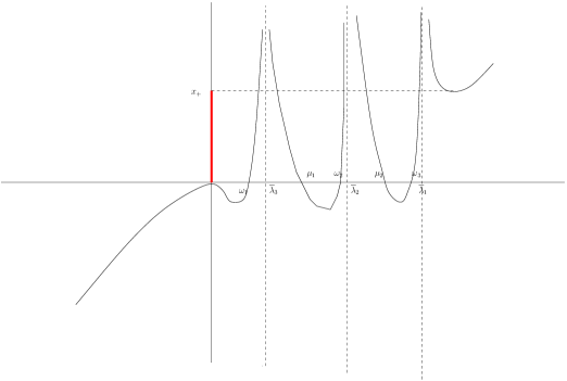
We illustrate such a behaviour when . In the context of Fig. 1, the support is reduced to the single interval because for .
In order to precise the support when vanishes in , we need to characterize the corresponding zeros. For this, we first justify that cannot have a multiplicity 2 zero. Assume for example that has a multiplicity 2 zero in , and denote by this zero. Then, if , the equation has simple real roots, and the multiplicity 3 root . Therefore, the equation has roots (counting multiplicities), a contradiction. We now establish the following useful result.
Proposition 12
The number of local extrema of in is an even number, say , with . If , we denote the arguments of these extrema by , then verify
| (8.60) |
Moreover, for each , the interval contains at most one interval , and (resp. ) is a local minimum (resp. local maximum) of .
Proof. We establish that if such that , the images and are also satisfy . The goal is to show that ratio is always positive. For more convenience we put for . With this and (8.58) we can rewrite
| (8.61) |
where . Let us notice that extremes and are by definition such that and are negative. Using directly (8.61) for and we can write
| (8.62) |
With the definition of the first term of (8.62) can be expended as
And similarly the second one as
Putting the last two equation in (8.62) we obtain
Now we recall that is positive as well as from what we have . That allows us to use the inequality
and to write
It is easy to check that . Using this we can rewrite last inequality as
| (8.63) |
Taking the derivatives of the expression (8.61), we obtain that . By definition, are extremes of function , i.e. . This gives immediately . After putting this into (8.63) and regrouping terms we obtain
Finally, we denote by the three parts of r.h.s and show that and can be presented as the sum of positive terms. Using again the definition of we expend as
Similarly, can be written as
This shows that , and that (8.60) holds. It remains to justify that each interval contains at most one interval .
Assume that the interval contains 2 intervals
and with . Then,
it also holds that .
is necessarily a local minimum because while
must be a local maximum. The same property holds for and .
However, this contradicts the property . This completes the proof of
Proposition 12.
Proposition 12 allows to identify the support .
Corollary 5
When , the support is given by
| (8.64) |
Proof. If belongs to the interior of the righthandside of (8.64), has only real solutions. This implies that the 2 remaining roots are complex valued, i.e. that . This leads to the conclusion that
and that
Conversely, if , the equation has real solutions, which implies that is real. Therefore,
or equivalently,
This completes the proof of Corollary (5).
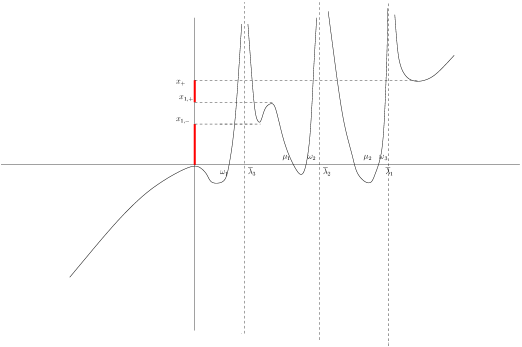
We illustrate the above behaviour when . In the context of Fig. 2, vanishes on and not on . The support thus coincides with .
When matrix is reduced to , i.e. and , the support of course coincides with , and is given by
| (8.65) |
Moroever, is equal to
| (8.66) |
(8.65) and (8.66) are in accordance with the results of [22].
We now briefly address the case . The behaviour of is essentially the same as if , except that the first root of the equation is now strictly negative. As , this implies that it exists for which . Moreover, this point is unique, otherwise, the equation would have more than roots for certain values of . is thus a local maximum of whose argument is strictly negative. We also notice that if . Apart these differences, the behaviour of for remains the same as if . In particular, Proposition 12 still holds true. However, we remark that if , the equation has still real solutions that are strictly positive, and 2 extra real roots, the smallest one being less than and the other one being negative and largest that . This implies that is real. We also notice that coincides with the smallest extra negative root because it satisfies conditions (8.59). Hence, the interval is included into . If does not vanish on , for , the equation has only real solutions that do not satisfy conditions (8.59) and 2 extra complex conjugates solutions. Therefore, and . Conversely, , which implies that . As it was established above that , we deduce that if does not vanish on . If vanishes on , i.e. if (we recall that is defined in Proposition 12), the support is given by
| (8.67) |
To justify this, we just need to establish that , and to use the same arguments as in the proof of Corollary 5. To justify , we put , and follow step by step the arguments used to evaluate . We notice that in contrast with the context of the proof of Corollary 5, and . However, is still negative, so that is still positive. This allows to conclude that all the inequalities used in the course of the proof of Corollary 5 remain valid, except the evaluation of the term that needs the following simple modification: we express as
As and are positive, it holds that
Therefore, , and holds.
In order to unify the cases and , we define for by , and summarize the above discussion by the following result.
Theorem 2
The support is given by
| (8.68) |
We now establish that sequences and are bounded. In other words, for each , the support is included into a compact interval that does not depend on .
Lemma 14
| (8.69) |
In order to prove this lemma, we use that and that . It is easy to check that
For , it is clear that . Writing that and , we obtain immediately that can be written as
where verifies and is a rational function of that does not depend on and which converges towards when . Therefore, for each , it exists such that for each . As and that , we obtain that for . As , we deduce from this that . As does not depend on , this establishes that . To prove that is bounded, we observe that . As , it is easily seen that
Therefore, sequences and are bounded. This completes the proof of Lemma 14.
We finally provide a sufficient condition under which the support is reduced to if and to if . More precisely, the following result holds.
Proposition 13
Assume that it exist such that for each large enough, the following condition holds:
| (8.70) |
for each pair , . Then, for each large enough, if and to if .
Proof. We assume that (8.70) holds, and that does not coincide with or , i.e. vanishes at a point such that and . After some algebra, we obtain that satisfies:
As , this implies that
Jensen’s inequality leads to . Therefore, we obtain that , and that
| (8.71) |
We assume that . Then, hypothesis (2.6) and condition (8.70) imply that
Hence, it must hold that
for each large enough, a contradiction because is easily seen to be an unbounded term.
9 No eigenvalues outside the support.
In this paragraph, we establish the following result:
Theorem 3
Assume that there exists , , and an integer such that
| (9.1) |
Then with probability one, no eigenvalues of appears in for all large enough.
We first remark that it is sufficient to consider the case where . To justify this claim,
we recall that is a compact subset (see Lemma 14), and notice that where matrix is defined
by (2.4). Moreover, (3.1)
implies that almost surely, for large enough,
where . Therefore, almost surely, the largest eigenvalue of
is for each large enough upperbounded by the nice constant .
This justifies that it is sufficient to assume that in the following.
In order to establish Theorem 3, we use the Haagerup-Thornbjornsen approach ([15], see also [6]). The crucial step of the proof is the following Proposition.
Proposition 14
we have for large enough,
| (9.2) |
where is holomorphic in and satisfies
| (9.3) |
for each , where and are nice polynomials.
Proof. To prove (9.2) we write
As (6.5) holds, it is sufficient to establish that
| (9.4) |
for some nice polynomial and . In the following, we denote by the function defined by
| (9.5) |
It is clear that . Moreover, if represents the associated positive measure, then we have
| (9.6) |
(9.6) can be proved using the arguments of the proof of Proposition 5.
As is given by (7.23) for , (9.4) appears equivalent to the property
| (9.7) |
In order to prove (9.7), we define the following functions that appear formally similar to functions and defined by (7.13) and (7.14):
| (9.8) | |||
| (9.9) | |||
| (9.10) | |||
| (9.11) |
Using equation and the definition of and , we obtain easily that
| (9.12) |
holds, where
| (9.13) | |||
| (9.14) | |||
| (9.15) |
This can also be written as
| (9.16) |
(6.4) leads to . In order to verify that are
as well, we have to control and . As and are
terms, it is sufficient to evaluate the denominator of the right handside of (9.10). As the mass and the first moment of and (the measure
associated to ) both verify the conditions of Lemma 5,
this Lemma implies that and . Therefore, we have checked that are terms.
In order to evaluate , it is of course necessary to show that matrix is invertible on , and to control the action of its inverse on the vector . We define matrix by
| (9.17) |
and establish the following result.
Lemma 15
For each , it exist nice constants and such that
| (9.18) |
Moreover, it exist 2 nice polynomials and for which
| (9.19) |
and
| (9.20) |
for each , where is defined as
| (9.21) |
Finally, for each , it holds that
| (9.22) |
Proof. To evaluate , we use the calculations of the proof of Lemma 7. In particular, we have
| (9.23) |
This implies that
| (9.24) |
By applying Cramer’s rule to (9.23), we obtain that
| (9.25) |
It is clear that . Therefore, it holds that . We now evaluate . For this, we remark that
| (9.26) |
Jensen’s inequality implies that . Therefore, the application of Lemma 5 to implies that
for some nice constants and . (9.18) thus follows from (9.25).
We now establish (9.19) and (9.20), and denote by the function . Using the equation , and calculating and , we obtain immediately that
| (9.27) |
The first component of (9.27) leads to
| (9.28) |
Using the same arguments as above, we obtain that . As (9.6) holds, we can apply Lemma 5 to and obtain as above that
for some nice constants and . We remark that . Therefore, by Lemma 5 applied to , it holds that for some nice constants and . As for some nice polynomials and ,we obtain that
| (9.29) |
if belongs to the set defined by
The set is clearly defined in the same way than , but from 2 other nice polynomials and .
Using the Cramer rule, we obtain that can be written as
| (9.30) |
Plugging (9.29) in the last equation, we get that the inequality
| (9.31) |
holds for each . As , we obtain that
for each , where is defined as from
2 nice polynomials and . We put and
, and consider the set defined by
(9.21). It is clear that ,
and that (9.19) and (9.20) hold if .
It remains to establish (9.22). For this, we remark that the inequalities
hold for each . Therefore, (9.22) follows
from (9.18) and (9.20). This completes
the proof of Lemma 15.
Solving (9.16), we obtain immediately that it exists 2 nice polynomials and such that,
holds for each . If , we use the argument in [15]. More precisely, if , the inequality holds. As on , we deduce that
for each . This, in turn, leads to the conclusion that for each . This establishes (9.7) and as expected. This completes the proof of Proposition 14.
Lemma 16
Let be a compactly supported real valued smooth function defined on , i. e. . Then,
| (9.32) |
Proof. Due to Proposition 3 we can write
| (9.33) |
as well as
| (9.34) |
Using Proposition 14, we obtain
| (9.35) |
Since the function , we can use the result which was proved in [6, Section 3.3] and obtain
| (9.36) |
for some nice constant . This and (9.35) complete the proof.
In order to establish Theorem 3, we introduce a function such that and
Since for large enough then and according to Lemma 16
Now we show that
For this we use again the Poincare-Nash inequality
We only evaluate the first term of the r.h.s. of the inequality, denoted by , because the second is similar. For this we write first
Plugging this into (3) we obtain
Following the proof of Lemma 1, we obtain
| (9.37) |
To evaluate the first term () of the r.h.s of (9.37) we denote and write
We recall that (3.1) implies that . Therefore, it holds that
Lemma 16 implies that . Throughout the proof of Lemma 1, we get that for all . Since function , there exists a nice constant such that for all and for all . We deduce from this it exists a nice constant such that for each . From what about we conclude that .
As for the second term () of the r.h.s of (9.37), we write
It is easy to see that can be evaluated as , leading to the conclusion that . Therefore, we have checked that
Now we can complete the proof of Theorem 3 as in [7]. For this we apply the classical Markov inequality and combine what above
Applying Borel-Cantelli lemma, for large enough, we have with probability one
By the very definition of function , the number of eigenvalues of matrix lying in the interval is upper bounded by . Since this number of eigenvalues is an integer, we conclude that with probability one there is no eigenvalues in the interval for each large enough.
We finally illustrate the above results by the following numerical experiment. are given by , and so that . The eigenvalues of matrix are defined by for . Matrix verifies . Fig. 3 represents the histogram of the eigenvalues of a realization of as well as the graph of the density . We notice that the histogram and the graph of are in accordance, and that, as expected, no eigenvalue of lies outside the support of .
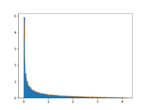
10 Recovering the behaviour of the empirical eigenvalue distribution using free probability tools
The purpose of this paragraph is to show that it is possible to use free probability tools in order
to characterize the limiting behaviour of the empirical eigenvalue distribution of matrix
. As the present paper is not focused on these kind of approach, we present briefly the following results and leave the details to the reader.
The free probability approach is based on the following observations:
-
•
Up to the zero eigenvalue, the eigenvalues of coincide with the eigenvalues of
-
•
The matrices and are almost surely asymptotically free. Therefore, the eigenvalue distribution of converges towards the free multiplicative convolution product of the limit distributions of and . These two distributions appear to coincide both with the limit distribution of the well known random matrix model where is a complex Gaussian random matrix with unit variance i.i.d. entries.
In the following, we follow the definitions of asymptotic freeness provided in [19]
(see in particular section 4.3) which need the existence of certain limit distributions. This is in contrast with
the approach developed in the previous sections more focused on the behaviour of deterministic equivalents. We however mention that more recent free probability works (see e.g. [29] and the references therein, [5]) allow to avoid the introduction of limit distributions, and would allow to recover the previous results on the deterministic equivalent of .
In order to be in accordance with [19], we thus formulate in this section the following assumption:
Assumption 1
The empirical eigenvalue distribution of matrix converges towards a limit distribution
We remark that hypothesis 2.6 implies that is compactly supported. Moreover, it can be shown that measures and both converge weakly towards limits denoted and in this section. We also notice that Lemma 14 implies that and are compactly supported. It is also easily checked that the Stieltjes transform of verifies the equation
| (10.1) |
while the Stieltjes transform of is given by
| (10.2) |
We recall that represents the limit of . In the following, we establish that
(10.1) and (10.2) can be obtained using free probability
technics.
Before going further, we first recall the main useful definitions introduced in [19].
Definition 1
Consider a finite family of sequences of possibly random matrices . Then is said to have an almost sure joint limit if for each non commutative polynomial in indeterminates, then converges almost surely towards where is a deterministic distribution defined on the set of all non commutative polynomials in indeterminates (i.e. is a linear form such that ).
We remark that if and are Hermitian matrices, the above condition is equivalent to the existence of a limit empirical eigenvalue distribution.
Definition 2
Consider families of possibly random matrices. Then, are said to be almost surely asymptotically free if the 2 following conditions hold:
-
•
For each , has an almost sure joint limit
-
•
, with , and for each non commutative polynomials in indeterminates such that a.s. it holds that
(10.3)
We remark that when each family is reduced to a single sequence of hermitian, or similar to hermitian matrices 222in the sense that for some hermitian matrix , the almost sure freeness of holds if
Definition 3
-
•
For each , has a limit eigenvalue distribution
-
•
, with , and for each 1 variate polynomials such that a.s. it holds that
(10.4)
We also recall the definition of the transform of a probability measure, and recall that the transform of the free multiplicative convolution product of 2 probability measures is the product of their transforms.
Definition 4
Given a compactly supported probability measure carried by , we define as the formal power series defined by
| (10.5) |
Let be the unique function analytic in a neighbourhood of zero, satisfying
| (10.6) |
for small enough. The, we define the transform of as the function defined in a neighbourhood of zero by
| (10.7) |
Moreover, if and are two compactly supported probability measures carried by , the S-transform of satisfies
| (10.8) |
We are now in position to state the main result of this section.
Proposition 15
Matrices and are almost surely asymptotically free.
Proof. We first notice that it possible to replace matrices and by finite rank perturbations because the very definition of almost sure asymptotic freeness is not affected by finite rank perturbations. We thus exchange and by and where and are defined by
| (10.9) |
| (10.10) |
In other words, vectors are replaced by vectors . In order to simplify the notations, we still denote the above finite rank modifications by . We define the matrix and matrix by
| (10.11) |
and rewrite (and respectively) as
| (10.12) |
This allows us to obtain the useful expression for and
| (10.13) | |||
| (10.14) |
Since can be written as , where has i.i.d. Gaussian entries, the hermitian matrix is unitarily invariant. Moreover, Assumption 1 implies that has a limit distribution while it is easily checked that the family has the same property. This and Theorem 4.3.5 in [19] leads to the conclusion that and are almost surely asymptotically free. Proposition 15 thus appears to be an immediate consequence of the following Lemma adapted from Lemma 6 in [13]. In order to make the connections between Lemma 17 and Lemma 6 in [13], we use nearly the same notations than in [13] in the following statement.
Lemma 17
We consider a sequence of hermitian random matrices and deterministic matrices such that and are almost surely asymptotically free. Then, if satisfy
| (10.15) |
for each as well as for all , then the random matrices are almost surely asymptotically free.
Proof. We prove Lemma 17 by following step by step the proof from [13]. For simplicity we omit index below. Due to (10.15) we have so that matrices are similar to the hermitian matrix . We have thus to verify the 2 items of Definition 3. The first item is obvious. To check condition (10.4), we consider any , indexes with and polynomials such that a.s. Using again (10.15) it is clear that and, as a consequence, a.s. We define as
where . If then by assumption for . As we also have a.s, the almost sure asymptotic freeness of and leads to the conclusion that a.s. In the case when we have and the same conclusion holds.
By taking , and , Lemma 17 gives us immediately that
are almost surely asymptotically free. Using the expression (10.13, 10.14) of and , we obtain that and are almost surely asymptotically free.
We also deduce that the limit distributions of and both coincide with the additive free convolution product of copies of the well known limit distribution of . It is easily seen that the Stieljes transform, denoted in the following, of this free addditive convolution product is solution of the familiar equation
| (10.16) |
In the following, we denote by the corresponding probability measure.
It is clear that (10.16) coincides with the equation verified by the Stieltjes transform of the limit eigenvalue distribution
of the random matrix where is a complex Gaussian random matrix with unit variance i.i.d. entries.
We note that this result could also be easily obtained using the Gaussian technics developed in [26] in the case where is reduced to a multiple
of .
According to Proposition 15, the limit eigenvalue distribution of is . In the following, we denote by this measure and by its Stieltjes transform. To find an equation satisfied by , we use (10.8). (10.7) and (10.8) give us immediately
By replacing here with and taking into account (10.6) we obtain
| (10.17) |
We notice that by definition (10.5), we have
| (10.18) |
Putting this into (10.17) and replacing with give us
From this, it is straightforward to obtain the expression of . For more convenience, we introduce the function which is analytic in the neighbourhood of infinity. It holds that
| (10.19) |
It remains to determine . For this we use (10.18) for , and replace with . Then (10.6) gives
To obtain the equation for it is sufficient to use the above expression of , and to plug it in (10.16) with . Therefore, we obtain that
After simple algebra we get that
We finally replace by . With (10.17) it is easy to see that the l.h.s. equal to . To treat the r.h.s. we use again (10.17) to obtain that , and get that
| (10.20) |
Now we recall the equation obtained above for
| (10.21) |
The equations (10.20) and (10.21) are identical up to factor . Since it can be shown that Eq. (10.21) has a unique solution on the set of Stieltjes transforms, we obtain that . Therefore, (10.19) leads to the equation
The Stieltjes transform of the limit eigenvalue distribution of is clearly equal to . Using the expression (10.2) of , we obtain immediately that
We have thus proved that the limit eigenvalue distribution of can be evaluated using free probability technics.
Acknowledgments
The authors thank warmly Prof. Leonid Pastur for fruitful discussions.
References
- [1] M. Bhattachargee, A. Bose, “Large sample behaviour of high-dimensional autocovariance matrices”, Ann. Statist., vol. 44, no. 2, pp. 598-628, 2016a.
- [2] A. Bose, M. Bhattachargee, “Large Covariance and Autocovariance Matrices”, Monographs on Statistics and Applied Probability 162, CRC Press, 2019.
- [3] F. Benaych-Georges, R.R. Nadakuditi, ”The eigenvalues and eigenvectors of finite, low rank perturbations of large random matrices”, Adv. in Math., 227(1):494-521, 2011
- [4] F. Benaych-Georges, R.R. Nadakuditi,”The singular values and vectors of low rank perturbations of large rectangular random matrices”, J. Multivariate Anal., vol. 111 (2012), pp. 120-135.
- [5] S. Belinschi, M. Capitaine, “Spectral properties of polynomials in independent Wigner and deterministic matrices”, Journal of Functional Analysis, Volume 273, Issue 12, pp 3901-3963 (2017).
- [6] M. Capitaine, C. Donati-Martin, “Strong asymptotic freeness of Wigner and Wishart matrices,” Indiana Univ. Math. Journal, vol. 56, pp. 295–309, 2007.
- [7] M. Capitaine, C. Donati-Martin, and D. Féral, “The largest eigenvalue of finite rank deformation of large Wigner matrices: convergence and non-universality of the fluctuations,” Annals of Probability, vol. 37, no. 1, pp. 1–47, 2009.
- [8] H. Cartan, “Théorie élémentaire des fonctions analytiques d’une ou plusieurs variables complexes”, Hermann, 1978.
- [9] F. Chapon, R. Couillet, W. Hachem, X. Mestre, ”The outliers among the singular values of large rectangular random matrices with additive fixed rank deformation” , Markov Processes and Related Fields, 20, 183–228 (2014).
- [10] A. Ciuso, G. Picci, ”Asymptotic variance of subspace estimates”, J. of Econometrics 118 (1-2):257-291, February 2004.
- [11] R. Couillet, ”Robust spiked random matrices and a robust G-MUSIC estimator”, Elsevier Journal of Multivariate Analysis, vol. 140, pp. 139-161, 2015.
- [12] B. Dozier, J. Silverstein, ”On the Empirical Distribution of Eigenvalues of Large Dimensional Information-Plus-Noise Type Matrices”, Journal of Multivariate Analysis, 98(4) (2007), pp. 678-694.
- [13] J. Evans, D. N. C. Tse, “Large System Performance of Linear Multiuser Receivers in Multipath Fading Channels,” IEEE Transactions on Information Theory, Vol. 46, No. 6, 2000.
- [14] F. Gesztesy, E. Tsekanovskii, “On matrix-valued Herglotz functions”, Math. Nach. 218 61-138, 2000.
- [15] U. Haagerup, S. Thorbjornsen, ”A new application of random matrices: is not a group”, Annals of Mathematics, 162(2):711, 2005.
- [16] W. Hachem, P. Loubaton, and J. Najim, ”Deterministic equivalents for certain functionals of large random matrices”, Annals of Applied Probability, 17(3):875–930, 2007.
- [17] W. Hachem, P. Loubaton, J. Najim, X. Mestre, P. Vallet ”A subspace estimator for fixed rank perturbations of large random matrices”, Journal of Multivariate Analysis, 114 (2013), pp. 427-447
- [18] F. Hansen, G.K. Pedersen, “Jensen’s operator inequality”, Bull. London Math. Soc. 35 (2003), 553-564
- [19] F. Hiai, D. Petz, ”Asymptotic freeness almost everywhere for random matrices”, Acta Sci. Math. (Szeged), 66/3–4 (2000), 809–834
- [20] R.A. Horn, C.R. Johnson, “Matrix Analysis”, Cambridge University Press, 1985.
- [21] B. Jin, C. Wang, Z.D. Bai, K.K. Nair, M. Harding, “Limited spectral distribution of a symmetrised auto-cross covariance matrices”, Ann. of Proba., vol. 24, no. 3, pp. 1199-1225, 2014.
- [22] Z. Li, G. Pan, J. Yao, ”On singular value distribution of large-dimensional autocovariance matrices”, J. Multivariate Analysis, vol. 137, pp. 119-140, May 2015.
- [23] Z. Li, Q. Wang, J. Yao, ”Identifying the number of factors from singular values of a large sample auto-covariance matrix”, to appear in Annals of Statistics, December 2016.
- [24] A. Lindquist, G. Picci, “Linear Stochastic Systems”, Series in Contemporary Mathematics, Vol. 1, Springer, 2015
- [25] H. Liu, A. Aue, D. Paul, “On the Marcenko-Pastur law for linear time series”, Ann. of Stat., vol. 43, no. 2, pp. 675-712, 2015.
- [26] P. Loubaton, ”On the almost sure location of the singular values of certain Gaussian block-Hankel large random matrices”, Journal of theoretical probability, May 2015.
- [27] C. Male, “The norm of polynomials in large random and deterministic matrices”, Probability Theory and Related Fields (2012) DOI: 10.1007/s00440- 011-0375-2.
- [28] Mestre, X. and Lagunas, M.A., ”Modified subspace algorithms for DoA estimation with large arrays”, IEEE Transactions on Signal Processing, vol. 56, no. 2, pp. 598-614, February 2008.
- [29] J. Mingo, R. Speicher, “Free Probability and Random Matrices”, Fields Institute Monographs, Springer, 2017.
- [30] R.R. Nadakuditi, A. Edelman, ”Sample eigenvalue based detection of high-dimensional signals in white noise using relatively few samples”, IEEE Trans. Signal Processing, vol. 56, no. 7, pp. 2625-2637, Jul. 2008.
- [31] R.R. Nadakuditi, J.W Silverstein, ”Fundamental limit of sample generalized eigenvalue based detection of signals in noise using relatively few signal-bearing and noise-only samples”, IEEE J. Sel. Topics Signal Processing, vol. 4, no. 3, pp. 468 -480, Jun. 2010.
- [32] L.A. Pastur, M. Shcherbina, ”Eigenvalue Distribution of Large Random Matrices”, Mathematical Surveys and Monographs, Providence: American Mathematical Society, 2011.
- [33] D. Paul, “Asymptotics of sample eigenstruture for a large dimensional spiked covariance model”, Statistica Sinica, Vol. 17, No. 4, 1617-1642, 2007.
- [34] J. W. Silverstein, and S. I. Choi, ”Analysis of the limiting spectral distribution of large dimensional random matrices”, J. Multivariate Anal. 54. 295-309.(1995).
- [35] G.T. Pham, P. Loubaton, P. Vallet, ”Performance analysis of spatial smoothing schemes in the context of large arrays”, IEEE Trans. on Signal Processing, vol. 64, no. 1, pp. 160-172, January 2016.
- [36] P. Van Overschee, B. de Moor, ”Subspace Identification for Linear Systems: Theory, Implementation, Applications”, Kluwer Academic Publishers, 1996.
- [37] J. Vinogradova, R. Couillet, and W. Hachem, ”Estimation of Toeplitz covariance matrices in large dimensional regime with application to source detection”, IEEE Transactions on Signal Processing, 63 (18), pages 4903-4913, September 2015.
- [38] J. Vinogradova, R. Couillet and W. Hachem, ”Statistical Inference in Large Antenna Arrays under Unknown Noise Pattern”, IEEE Transactions on Signal Processing, 61 (22), 2013, pages 5633-5645.
- [39] D. Voiculescu, K. J. Dykema, A. Nica, ”Free Random Variables”, ser. CRM Monograph. Providence, RI: Amer. Math. Soc., 1992, vol. 1.
- [40] D. Voiculescu, ”Lectures on Free Probability Theory”, in unpublished Notes for a Course at the Saint-Flour Summer School on Proability, 1998.