A geometric alternative to dark matter

Abstract

The existence of “dark matter”, inferred from the observed rotation curves of galaxies, is a hypothesis which is widely regarded as problematic. This paper proposes an alternative hypothesis based on the space-time geometry near a rotating body and formulated in terms of the dragging of inertial frames. This hypothesis is true in a certain linear approximation to General Relativity (Sciama [9]) and is justified in general by Mach’s principle. Dark matter corrects the rotation curve but does not predict the ubiquitous spiral structure of galaxies. The geometric alternative suggested here deals with both problems and allows the construction of a simple model for the dynamics of spiral galaxies which fits observations well.

1 Introduction

One of the major problems with the current consensus model for the universe is the problem of dark matter which has no observations to support its existence and no agreement as to its nature. The purpose of this paper is to propose an alternative based on the geometry of space-time, which, like dark matter, explains observed rotation curves. There is a dual problem to the dark matter problem, namely the spiral structure problem. In the current consensus model for the universe, with dark matter, there is no satisfactory model for galactic dynamics that explains the ubiquitous spiral form of many galaxies. By contrast the geometric postulate made here fits observed rotation curves and also provides a good model for galactic dynamics fitting observed spiral structure.

Dragging of inertial frames, henceforth abbreviated to “inertial drag” or ID, is a relativistic effect whereby the non-inertial motion of a body (acceleration and$/$or rotation) causes the inertial frames at other points to be dragged. In his thesis [9] Sciama proposed that this effect should embody Mach’s principle (that inertial frames depend on the total distribution of matter in the universe) and that this should specify the full dynamics of the universe. He illustrated this with a special case (a certain linear approximation to general relativity) where it all works perfectly. His formula for the ID effect of a rotating body is this:

Weak Sciama Principle (WSP)A mass $M$ at distance $r$ from a point $P$, rotating with angular velocity $\omega$, contributes a rotation of $k\mkern 2.0muM\mkern 2.0mu\omega/r$ to the inertial frame at $P$ where $k$ is constant.

It is called the “Sciama principle” to distinguish it from the more general “Mach principle” and “weak” because it specifies only the effect of one rotating body, instead of all non-inertial motions. The “Full Sciama Principle” (for rotation) states that the rotation of a local inertial frame is obtained by adding the effects for all rotating bodies in the accessible universe (ie not regressing faster than $c$).

The factor $k\mkern 2.0muM/r$ must be regarded as a weighting factor and the sum must be divided by the sum of the weights. For an example see the derivation of (1) below.

This principle (the WSP) is the proposed geometric hypothesis. The key factor for the rotation curve is $1/r$ which has several pieces of evidence in its favour. It fits Sciama’s approximation. It fits the behaviour of apparent acceleration (see Mach [6, Ch II.VI.7 (page 286)]). There is a simple dimensional argument that supports it (see the discussion of the precession of the Foucault pendulum in Misner, Thorne and Wheeler [7] starting on page 547 para 3 with the margin note The dragging of the inertial frame).

The hypothesis is obviously related to Mach’s principle though it is much weaker. But it has the advantage that it is capable of direct verification by observation. Although true in an approximation to general relativity (GR), it is not true in general in GR: in the Kerr metric, ID drops off with $1/r^{3}$ not $1/r$. Therefore to accomodate it within GR it is necessary to assume that a rotating body has an effect on the local field that causes the hypothesised ID effect and stops it being a vacuum. This effect embeds Mach’s principle (for rotation) within GR and avoids the paradoxes that arise in a naive formulation of the principle: the ID field is a form of gravitational disturbance that propagates, like all gravitational disturbances, at the speed of light.

2 The rotation curve

The basic assumption is that the centre of every galaxy contains a heavy rotating mass (presumably a black hole). It is the ID effects from this mass that cause equatorial orbits to exhibit the characteristic rotation curve. However, the analysis applies to any axially-symmetric rotating body, which does not need to be assumed to be heavy.

To fix notation, consider a central mass $M$ at the origin in $3$–space which is rotating in the right-hand sense about the $z$–axis (ie counter-clockwise when viewed from above) with angular velocity $\omega_{0}$. Assume a flat background space-time, away from $M$, with sufficient fixed masses at large distances to establish a non-rotating inertial frame near the origin, if the effect of $M$ is ignored. Let $P$ be a point in the equatorial plane (the $(x,y)$–plane) at distance $r$ from the origin. The rotation of the inertial frame at $P$ is given by adding the contribution from $M$ to the contribution from the distant masses. The inertial frame at $P$ is rotating coherently with the rotation of $M$ by the average of $\omega_{0}$ weighted $kM/r$ and zero (for the distant fixed masses) weighted $C$ say. Normalise the weighting so that $C=1$ (which is the same as replacing $k/C$ by $k$) which leaves just one constant $k$ to be determined by experiment or theory. The nett effect is a rotation of

(1) $$\frac{(kM/r)\times\omega_{0}+1\times 0}{(kM/r)+1}=\frac{A}{r+K}\ \ \text{where}\ \ K=kM\ \ \text{and}\ \ A=K\omega_{0}.$$

NoteIf the full Sciama principle is assumed then $k=1$, $K=M$ and $A=M\omega_{0}$. However the choice of $k=1$ is not relevant to the arguments presented in this paper. Nothing that is proved depends on knowing the exact relationship between $K$ and $M$. When constructing models for galaxies in sec:dyn the value $k=1$ will be used for definiteness and to the extent that these models fit observations of real galaxies this provides evidence for the full Sciama principle.

The key to the rotation curve is to understand the way in which the inertial drag field affects the dynamics of particles moving near the origin. For simplicity work in the equatorial plane and in a linear approximation to a background Minkowski space. Further assume a Newtonian formula for the central attractive force. For more accuracy, an approximation to a Schwarzschild space should be used, but the Minkowski–Newton approximation is reasonably accurate away from the centre and gives good results for the orbits. Assume that the inertial frame at $P$ (at distance $r$ from the origin) is rotating with respect to the background with angular velocity $\omega(r)$ counter-clockwise. When computing rotation curves, the formula for $\omega(r)$ just found (1) will be used but for the present discussion it is just as easy to assume a general function. The inertial frame at $P$ can be identified with the background space, but it is important to remember that it is rotating. There is no sensible meaning to the centre of rotation for an inertial frame. Two rotations which have the same angular velocity but different centres differ by a uniform linear motion and inertial frames are only defined up to uniform linear motion. Thus it can be assumed for simplicity that all the rotations have centre at the origin. Then the inertial frames can be pictured as layered transparent sheets, each comprising the same point-set but with each one rotating with a different angular velocity about the origin. Each sheet corresponds to a particuar value of $r$. It is necessary to be very clear about the nature of motion in one of these frames. A particle moving with a frame (ie one stationary in that frame) has no inertial velocity and its velocity is called rotational. In general if a particle has velocity $\mathbf{v}$ (measured in the background space) then

$$\mathbf{v}=\mathbf{v}_{\rm rot}+\mathbf{v}_{\rm inert}$$

where its rotational velocity $\mathbf{v}_{\rm rot}$ is the velocity due to rotation of the local inertial frame and $\mathbf{v}_{\rm inert}$ is its inertial velocity which is the same as its velocity measured in the local inertial frame. Note that $\mathbf{v}_{\rm rot}=r\omega(r)$ directed along the tangent.

Inertial velocity correlates with the usual Newtonian concepts of centrifugal force and conservation of angular momentum.

The fundamental relation

As a particle moves in the equatorial plane it moves between the sheets so that a rotation about the origin which is rotational in one sheet becomes partly inertial in a nearby sheet. For definiteness, suppose that $\omega(r)$ is a decreasing function of $r$ and consider a particle moving away from the origin and at the same time rotating counter-clockwise about the origin. The particle will appear to be being rotated by the sheet that it is in and this causes a tangential acceleration. This acceleration is called the slingshot effect because of the analogy with the familiar effect of releasing an object swinging on a string. But at the same time the particle is moving to a sheet where the rotation due to inertial drag is decreased and hence part of the tangential velocity becomes inertial and is affected by conservation of angular momentum which tends to decrease the angular velocity. These two effects balance each other out in the limit and this explains the flat asymptotic behaviour. More precisely, let $v$ be the tangential velocity of the particle in the direction of $\omega$ then the slingshot effect causes an acceleration $dv/dr=\omega(r)$ but conservation of angular momentum that operates on the inertial part of $v$, namely $v-r\mkern 2.0mu\omega(r)$ causes a deceleration in $v$ of $(v-r\mkern 2.0mu\omega(r))/r$ or an acceleration $dv/dr=\omega(r)-v/r$ and adding the effects we have the fundamental relation between $v$ and $r$:

(2) $$\framebox{$\displaystyle\frac{dv}{dr}=2\omega-\frac{v}{r}$}$$

Given $\omega$ as a function of $r$, (2) can be solved to give $v$ as a function of $r$. Rewrite it as

$$r\,\frac{dv}{dr}+v=2\omega r\,.$$

The LHS is $d/dr\,(rv)$ and the general solution is

(3) $$v=\frac{1}{r}\Bigl{(}\int 2\omega r\,dr+\text{const}\Bigr{)}.$$

It is now clear that any prescribed differentiable rotation curve can be obtained by making a suitable choice of continuous $\omega$.

RemarkIt is worth remarking that the fundamental relation does not depend on the WSP. It is a purely geometric result depending only on axial symmetry and the fact that the dynamic is controlled by a central force. It is true in any metrical theory and in particular in general relativity without the WSP. However for the models constructed here it will be used with the formula for $\omega$ found in (1) which does depend on the WSP.

Of interest here are solutions which, like observed rotation curves, are asymptotically constant, and, inspecting (3), this happens precisely when $\int 2\omega r\,dr$ is asymptotically equal to $Qr$ for some constant $Q$. But this happens precisely when $2\omega$ is asymptotically equal to $Q/r$. This proves the following result.

Theorem.

The equatorial geodesics have tangential velocity asymptotically equal to constant $Q$ if and only if $\omega$ is asymptotically equal to $A/r$ where $Q=2A$.

The basic model

Now specialise to the case $\omega=A/(r+K)$ which gives the value of inertial drag formulated in (1).

From (3)

$$v =\frac{1}{r}\left(\int\frac{2Ar}{r+K}\,dr+C\right)=\frac{2A}{r}\left(\int 1-\frac{K}{r+K}\,dr\right)+\frac{C}{r}$$

(4) $$=2A-\frac{2AK}{r}\log\left(\frac{r}{K}+1\right)+\frac{C}{r}\vrule width=0.0pt,height=20.0pt$$

where $C$ is a constant depending on initial conditions. For a particle ejected from the centre with $v=r\omega_{0}$ for $r$ small, $C=0$, and for general initial conditions there is a contribution $C/r$ to $v$ which does not affect the behaviour for large $r$. For the solution with $C=0$ there are two asymptotes. For $r$ small, $v\approx r\omega_{0}$ and the curve is roughly a straight line through the origin. And for $r$ large the curve approaches the horizontal line $v=2A$. A rough graph is given in fig:modbeg (left) where $K=A=1$. The similarity with a typical rotation curve, fig:modbeg (right), is obvious. Note that no attempt has been made here to use meaningful units on the left. See fig:rotsmod below for curves from the model using sensible units.

But notice that every equatorial orbit has the salient feature of observed rotation curves, namely a horizontal asymptote. This asymptote is the same for all equatorial orbits and hence any average over many orbits will also have this asymptote and this explains the observed rotation curve.

2 [r] at 14 457 1 [r] at 14 247 10 [t] at 130 17 20 [t] at 252 17 30 [t] at 364 17 40 [t] at 463 17   

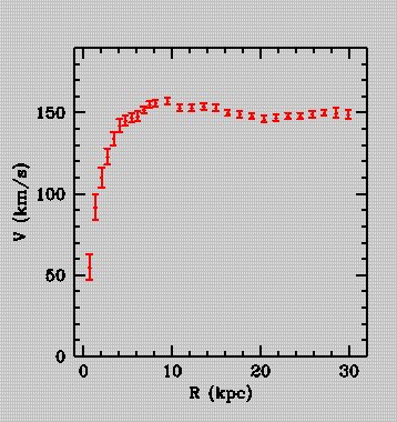
Figure 1: The rotation curve from the model (left) and for the galaxy NGC3198 (right) taken from Begeman [4]

Units

The models for the rotation curve and for galactic dynamics given in this paper are fully quantitative using natural units, in which $G$ (Newton’s gravitational constant) and $c$ (the velocity of light) are both $1$. Time is measured in years, distances in light-years, velocities in fractions of $c$ and mass converted into distance using the Schwarzschild radius: a mass of 1 means a mass with Schwarzschild radius 1 (light-year). Thus a velocity of .001 is $300\mathrm{km/s}$, a distance of 45,000 is 15Kpc and a mass of 1 is $3\times 10^{12}$ solar masses all approximately. When using natural units, pure numbers are used. They can be converted into more familiar units as indicated here.

There are other shapes for rotation curves; see [10] for a survey. All agree on the characteristic horizontal straight line. fig:rotsSR is reproduced from [10] and gives a good selection of rotation curves superimposed. In fig:rotsmod is a selection of rotation curves again superimposed, sketched using MathematicaThe notebook Rots.nb used to draw this figure can be collected from [2] and the values of the parameters used read off. and the model given here. The central masses for the curves in fig:rotsmod vary from $3\times 10^{11}$ to $10^{14}$ solar masses. The different curves correspond to choices of $A,K$ and $C$. The similarity is again striking.

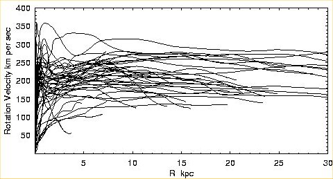
Figure 2: A collection of rotation curves from [10]

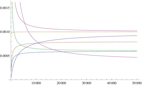
Figure 3: A selection of rotation curves from the model

It is worth commenting that the observed rotation curve for a galaxy is not the same as the rotation curve for one particle, which is what has been modelled here. When observing a galaxy, many particles are observed at once and what is seen is a rotation curve made from several different rotation curves for particles, which may be close but not identical. So it is expected that the observed rotation curves have variations from the modelled rotation curve for one particle, which is exactly what is seen in fig:modbeg (right) and fig:rotsSR.

Postscript

As remarked earlier, the effect described in this section is independent of mass. However for rotating bodies of small mass the effect is unobservably small. For example the sun has $K\approx\mathrm{3km}$ , assuming $K=M$, and $\omega_{\rm Sun}=2\pi/25$ days. Thus the asymptotic tangential velocity $2A=2K\omega_{\rm Sun}$ is $\mathrm{6km}$ per 4 days or $\mathrm{1m/s}$ approximately.

3 The full dynamic

The analysis given in sec:rot will now be extended to find equations for orbits in general (not just for the tangential velocity) and, using a hypothesised central generator, the spiral arm structure will be modelled as well. The basic idea is that the central mass accretes a belt of matter which develops instability and explodes feeding the roots of the arms. Stars are formed by condension in the arms and move outwards as they develop. Thus a typical star is on a long outward orbit and the rotation curve observed for stars in a spiral arm is formed of many such similar orbits. But this full picture is not necessary to explain the observed rotation curves, since the tangential velocity for all orbits has the same horizontal asymptote.

NoteThe assumption of a hypermassive central black hole in a spiral galaxy directly contradicts current beliefs of the nature of Sagittarius ${\rm A}^{*}$ and this problem together with other observational matters are dealt with in Chapter 6 of the book [8] of which this paper is a fragment. Very briefly, Sgr${\rm A}^{*}$ and the stars in close orbit around it form an old globular cluster near the end of its life with most of the matter condensed into the central black hole. It is not at the centre of the galaxy but merely roughly on line to the centre and it is about half-way from the sun to the real galactic centre which is invisible to us.

Plotting orbits

Equation (4) gave a formula for the tangential velocity in an orbit. What is needed is a formula for the radial velocity (again in terms of $r$) and these two will describe the full dynamic in the equatorial plane, which can then be used to plot orbits.

There are two radial “forces” on a particle: a centripetal force because of the attraction of the massive centre and a centrifugal force caused by rotation in excess of that due to inertial drag. Thus radial acceleration r̈ is given by

(5) $$\text{\em\"{r}}=\frac{v_{\inert}^{2}}{r}-F(r)$$

where $v_{\inert}=v-\omega r$ and $F(r)$ is the effective central “force” at radius $r$, per unit mass, which, since we are using a Newtonian approximation, is $M/r^{2}$. The same notation as in the last section is used here and in particular $\omega=\omega(r)$ is the inertial drag at radius $r$. Now specialise to the case $\omega=A/(r+K)$, equation (1), which was the formula for inertial drag coming from the Weak Sciama Principle. Here $A=K\omega_{0}$ and $K=kM$, where $M,\omega_{0}$ are the mass and angular velocity of the central mass, and $k$ is a weighting constant which can be taken to be 1 for purposes of exposition. The following formula for $v$, equation (4), was found:

(6) $$v=2A-\frac{2AK}{r}\log\left(\frac{r}{K}+1\right)+\frac{C}{r}\vrule width=0.0pt,height=20.0pt$$

where $C$ is a constant which can be read from the tangential velocity for small $r$. This implies:

(7) $$v_{\inert}=2A-\frac{2AK}{r}\log\left(\frac{r}{K}+1\right)+\frac{C}{r}\vrule width=0.0pt,height=20.0pt-\frac{Ar}{K+r}$$

Thus:

$$\text{\em\"{r}}=\frac{v_{\inert}^{2}}{r}-\frac{M}{r^{2}}=\frac{1}{r}\Bigg{[}2A-\frac{2AK}{r}\log\left(\frac{r}{K}+1\right)+\frac{C}{r}\vrule width=0.0pt,height=20.0pt-\frac{Ar}{K+r}\Bigg{]}^{2}-\frac{M}{r^{2}}$$

Multiplying by $\kern 2.0pt\dot{\kern-1.0ptr}$ and integrating with respect to $t$ gives

(8) $$\tfrac{1}{2}\kern 2.0pt\dot{\kern-1.0ptr}^{2}=\int\text{\em\"{r}}dr= -\frac{C^{2}}{2r^{2}}+\frac{M-2AC}{r}+\frac{A^{2}K}{K+r}+A^{2}\log(K+r)$$

$$+\frac{2AK(C+2Ar)\log(1+r/K)-(2AK\log(1+r/K))^{2}}{r^{2}}+E$$

where $E$ is another constant determined by the overall energy of the orbit. From this equation $\kern 2.0pt\dot{\kern-1.0ptr}$ can be read off (in terms of $r$). Moreover since there is a formula for $v$, there is also a formula for $\dot{\theta}=v/r$, where polar coordinates $(r,\theta)$ are used in the equatorial plane. From this it is possible to express $\theta$ and $t$ in terms of $r$ as integrals. These integrals are not easy to express in terms of elementary functions but Mathematica can be used to integrate them numerically and this can be used to plot the orbits of particles ejected from the centre. Now use the hypothesis that the centre of a normal galaxy contains a belt structure, which emits jets of gas$/$plasma, which condense into stars. The orbits of these stars can be modelled and a “snapshot” of all the orbits taken at an instant of time, in other words a picture of the galaxy can be given, fig:basic.

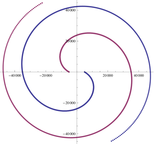
Figure 4: Mathematica plot using equations (8) and (6)

This compares well with classic observed spiral galaxies, fig:classic-spirals.

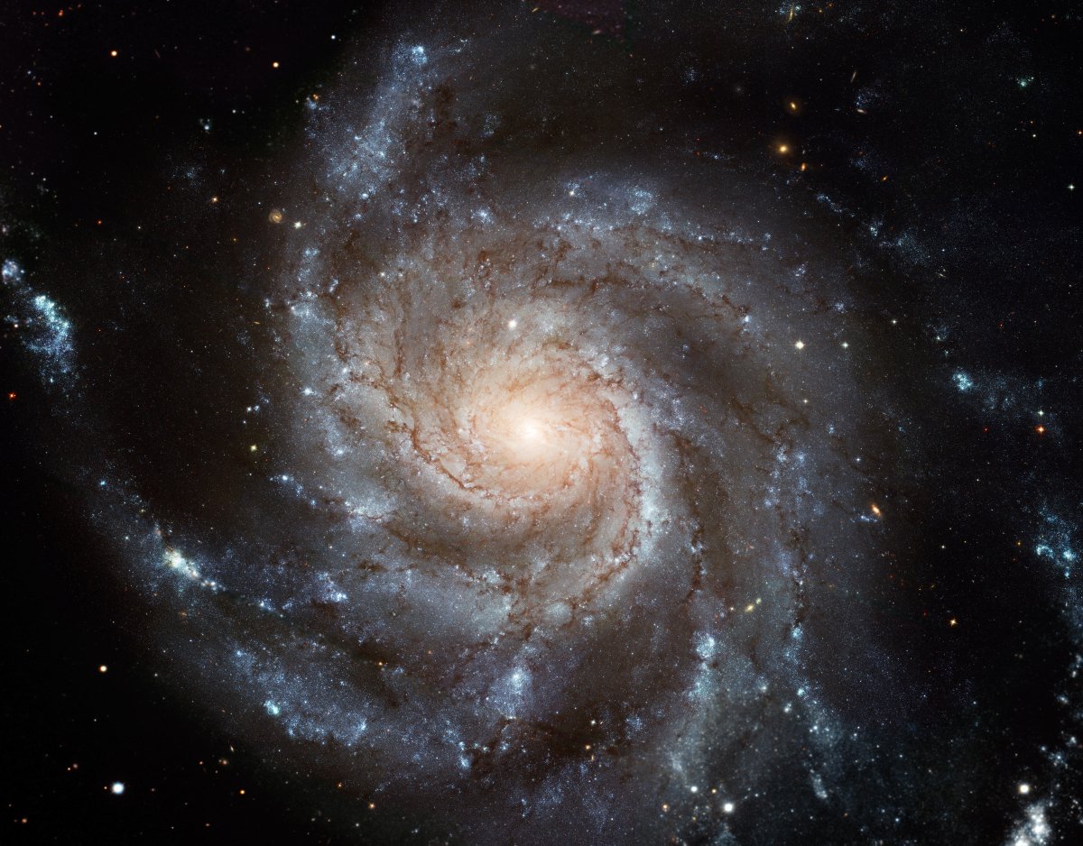
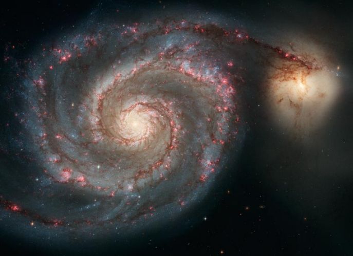
Figure 5: M101 (left) and M51 (right): images from the Hubble site [1]

To end this section it is worth remarking that it may be thought that motion along the arms is a new hypothesis and that observations should be able to verify this. However the observations aleady exist. The rotation curve shows that there is a general outward motion and, since the arms are close to tangential, as seen in the above figures, this motion is roughly along the arms, which is therefore already observed. The new hypothesis is that this motion is responsible for the long-term maintenance of the spiral structure. The model demonstrates all of this both graphically and quantitatively.

4 A new paradigm for the universe

As noted earlier, this paper is an extract from the author’s book “A new paradigm for the universe” [8], which covers all the topics discussed here in greater detail. The justification for the key factor $1/r$ in the main geometric hypothesisis is given in detail in [8, Chapter 2]. The derivation of the fundamental relation (2) and the radial acceleration equation (5) are both proved in detail for a larger class of suitable metrics in [8, Chapters 3 and 5]. The proposed accretion structure (the “generator”) which creates the jets which condense into the spiral arms is described in more detail in [8, Chapter 5]. The Mathematica notebook used for the plot, fig:basic, is typed out (and can be downloaded from [2] as Basic.nb) and the data used spelt out as follows.

$2A$ the asymptotic tangential velocity is $.001$ which is 300km/s in MKS units. $M$ has been set to $10^{11}$ solar masses. The minimum radius for the plot, rmin, has been set to 5,000 and the maximum, rmax, to 50,000 light years (corresponding to a visible diameter of 100,000 light years). There is a precession constant $B$ which arises because inertial drag causes the frame at the origin to appear to rotate at $A/$rmin and $B=A/$rmin corrects this and causes the familiar spiral form. Time elapsed along the visible arms is $5.5\times 10^{7}$ years. The nature of the visible spiral arms is discussed carefully in [8, Chapter 6]. Here merely note that the visible arms correspond to strong star-producing regions and bright short life stars, which burn out or explode in $10^{5}$ to $10^{7}$ years. Thus a total time elapsed of $5.5\times 10^{7}$ years allows several generations of stars to be formed and to create the heavy elements necessary for planets such as the earth to be formed.

RemarkThe rate of rotation of the central mass $\omega_{0}$ can be read from the other variables. Since $A=K\omega_{0}$, from equation (1), and the default value $K=M$ has been chosen, $\omega_{0}=A/M=.0005/.03=1/60$. In other words the central mass is rotating at about one radian every 60 years or one revolution every 360 year approx. This ought to be observable, but since the central mass in a galaxy is obscured by the bulge, all that can be observed are the velocities of stellar regions near the centre and these are dominated by the rotation curve. Since the correct rotation curve is built into the model, observations here are in agreement with the model.

The program is intended for interactive use and the reader is recommended to download a copy and investigate the output. Hints on using it can be found in [8, Section 5.6].

The book also covers a wide range of other topics and in particular gives a new framework for quasars, which fits with the observations of Halton Arp [3] and others, that quasars typically exhibit intrinsic redshift, and explains the apparently paradoxical results of Hawkins [5].

References

- [1] The Hubble site, http://hubblesite.org
- [2] Mathematica notebooks, available from\nlhttp://msp.warwick.ac.uk/~cpr/paradigm/Nb
- [3] H Arp, Sundry articles, available at\quahttp://www.haltonarp.com/articles
- [4] K C Begeman, H1 rotation curves of spiral galaxies, Astron Astrophys 223 (1989) 47--60
- [5] M R S Hawkins, On time dilation in quasar light curves, Mon Not Roy Astron Soc, 405 (2010) 1940--6
- [6] E Mach, The science of mechanics: a critical and historical account of its development, Translation from the original German by T J McCormack, Open Court Publishing Co (1893) (page numbers in the text refer to the sixth American edition (1960) Lib. Congress cat. no. 60-10179)
- [7] C W Misner, K S Thorne, J A Wheeler, Gravitation, Freeman (1973)
- [8] C Rourke, A new paradigm for the universe, arXiv:astro-ph/0311033
- [9] D Sciama, On the origin of inertia, Mon. Not. Roy. Astron. Soc. 113 (1953) 34--42
- [10] Y Sofue, V Rubin, Rotation curves of galaxies, Annu. Rev. Astron. Astrophys. 39 (2001) 137--174 \arxivastro-ph/0010594v2