Universal and non-universal text statistics: Clustering coefficient for language identification

Abstract

In this work we analyze statistical properties of 91 relatively small texts in 7 different languages (Spanish, English, French, German, Turkish, Russian, Icelandic) as well as texts with randomly inserted spaces. Despite the size (around 11260 different words), the well known universal statistical laws -namely Zipf and Herdan-Heap’s laws- are confirmed, and are in close agreement with results obtained elsewhere. We also construct a word co-occurrence network of each text. While the degree distribution is again universal, we note that the distribution of clustering coefficients, which depend strongly on the local structure of networks, can be used to differentiate between languages, as well as to distinguish natural languages from random texts.

Keywords Language Statistics  $\cdot$ Zipf’s Law  $\cdot$ Heaps’ Law  $\cdot$ Co-occurrence network  $\cdot$ Clustering coefficient  $\cdot$ Language identification

1 Introduction

Statistical characterization of languages has been a field of study for decades[1, 2, 3, 4, 5, 6]. Even simple quantities, like letter frequency, can be used to decode simple substitution cryptograms[7, 8, 9, 10, 11]. However, probably the most surprising result in the field is Zipf’s law, which states that if one ranks words by their frequency in a large text, the resulting rank frequency distribution is approximately a power law, for all languages [1, 12]. These kind of universal results have long piqued the interest of physicists and mathematicians, as well as linguists[13, 14, 15]. Indeed, a large amount of effort has been devoted to try to understand the origin of Zipf’s law, in some cases arguing that it arises from the fact that texts carry information [16], all the way to arguing that it is the result of mere chance [17, 18]. Another interesting characterization of texts is the Heaps-Herdan law, which describes how the vocabulary -that is, the set of different words- grows with the size of a text, the number of which, empirically, has been found to grow as a power of the text size [19, 20]. It is worth noting that it has been argued that this law is a consequence Zipf’s law. [21, 22]

A different tool used to characterize texts is the adjacency (or co-ocurrence) network [23, 24, 25, 26]. The nodes in this network represent the words in the text, and a link is placed between nodes if the corresponding words are adjacent in the text. These links can be directed -according to the order in which the words appear-, or undirected. In this work we study properties of the adjacency network of various texts in several languages, using undirected links. The advantage of representing the text as a network is that we can describe properties of the text using the tools of network theory [27]. The simplest characterization of a network is its degree distribution, that is, the fraction of nodes with a given number of links, and we will see that this distribution is also a universal power law for all languages. As we argue ahead, this may follow from the fact that Zipf’s law is satisfied.

Another interesting use for text statistics is to distinguish texts and languages. In particular, as occurs with letter frequencies, other more subtle statistics may be used to distinguish different languages, and beyond that, provide a metric to group languages into different families [28, 29, 30]. In this paper we use the clustering coefficient [27] to show that even though the degree distribution of the adjacency matrices is common to all languages, the statistics of their clustering coefficients, while approximately similar for various texts in each language, appears to be different from one language to another.

We use different texts (see Appendix (B)) instead of a large single corpus for each language because clustering coefficients typically decrease as a function of the size of the network[31]. Actually, we must compare the statistics of the clustering coefficient in texts with adjacency networks of comparable sizes. In the following section we present the rank vs frequency distribution for these texts. We also measure how the vocabulary increases with text size, as well as the respective degree distributions of the networks corresponding to every text, and compare them with a null "random" hypothesis. This null hypothesis consists of a set of texts constructed as follows: we select a text and remove all the spaces between words, then we reintroduce the spaces at random with the restriction that there cannot be a space next to another. We identify as words all strings of letters between consecutive spaces (the restriction avoids the possibility of having empty words). The reason we build the null hypothesis this way instead of the usual independent random letters with random spaces most commonly used [18, 32], is that consecutive letters are not independent: they are correlated to ensure word pronunciability, as well as due to spelling rules. Our method for constructing these random texts conserves most of the correlations between consecutive letters in a given language.

Next, we calculate the distribution of the clustering coefficients of the nodes of the adjacency network for each text. These distribution functions are more or less similar for all the texts of the same language, provided the networks are of the same size. However, it is apparent that the distributions are different between different languages. We also compare the clustering coefficient distributions with those of the null hypothesis. The data show that the strongest differences between languages occur for the fractions of nodes with clustering coefficients 0 and 1. We build a scatter plot for these fractions for all the texts in each language. Though there is overlap between some languages, other languages are clearly differentiated in the plot. We fit correlated bivariate gaussian distributions to the data of each language, which allows us to estimate a likelihood that a text is in a given language.

2 Texts and Universal laws

We analyzed 91 texts written in 7 languages: Spanish, English, German, French, Turkish, Russian and Icelandic. We also considered as null texts, 12 realizations of a randomized version the Portrait of Dorian Gray book, twice for each language analyzed here (except Icelandic). As mentioned above, the process for randomizing the text is as follows: first we remove the spaces in the original text. Then, we take the first letter, and with a probability of $1/2$ we add the next letter in the sequence, or the next letter in the sequence and a space. We advance to the last symbol added, and repeat the process until we reach the end of the text. This way we destroy the grammar of the original language, keeping the letter frequencies as well as most of the correlations between consecutive letters. The set of documents we used in this work are shown in Appendix B.

All texts were intervened to remove punctuation marks, numbers, parenthesis and other uncommon symbols, and all the letters were turned into lower case, so a word appearing with different case letters would not be counted as two different words. Also, we do not transliterate the texts, instead, we use the original symbols of the texts (Cyrillic alphabet for Russian texts or the special characters in Icelandic) using the UTF-8 encoding.

Also, since clustering coefficients depend non trivially on the size of the networks, we cut the texts so they all have essentially the same vocabulary size ($\simeq 11260$).

In table 1 we summarize for each language, the averages of the length, vocabulary size, maximum frequency and number of hapax legomena (i.e. words that appear only once in a document or corpus) of the texts studied here. It is important to note that for different languages, very different text lengths are required to achieve the same vocabulary size. We also note that in all cases, hapax legomena represent approximately half of the vocabulary in each text.

Language	Length	Vocabulary	Maximum Frequency	Number of Hapax
	$L$	$N_{tot}$	$f_{max}$	$H$
Spanish	85920	11253	4460	6265
English	219539	11258	11961	4582
French	90797	11260	4001	6302
German	78464	11264	2724	6590
Turkish	35392	11246	1173	7593
Russian	43799	11271	1726	7541
Icelandic	93699	11254	5063	6598
Random	63753	11258	4010	8340

Table 1: Averages for each language of the length, vocabulary size, maximum word frequency and number of hapax legomena of the texts studied in this work. Notice the large variations in text length required to achieve the same vocabulary size $N_{tot}$ from one language to another.

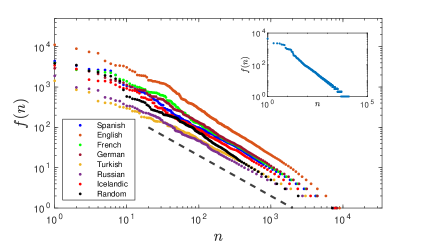
Figure 1: Word frequency $f(n)$ versus rank $n$ illustrating Zipf’s Law $f(n)\sim 1/n^{\alpha}$ for single randomly chosen texts in each language: English, Russian, Turkish, French, German, Spanish and Icelandic, using Log-binned data (colored symbols). Black dots represent the random texts constructed as described in the text. The dashed line corresponds to $\alpha=1$. In the inset we show an example of rank vs frequency plot without log-binning. Note that words with $f=1$ (hapax legomena) represent a large fraction of the vocabulary of the text

In figure (1) we show Zipf plots for some of the texts, including the random texts constructed as described previously. It is clear that all the texts reproduce convincingly Zipf’s law: $f(n)\sim 1/n^{\alpha}$ where $n=1,2,...N_{tot}$ is the word rank, $N_{tot}$ is the size of the vocabulary and $f(n)$ is its frequency. This is in contrast to previous work in which it is argued that there are differences between the Zipf plots of texts and random sequences[33], this might be due to the fact that our random text construction preserves correlations between letters, whereas the letters in [33] were placed independently. Our findings are summarized in Appendix (A).

Figure (1) is the typical rank vs frequency plot for a randomly chosen text in each language. From the figure, we see that $\alpha\simeq 1$, obtained by least squares fits to the plot, describes very well all the texts. Therefore, given that $n/N_{tot}$ is the fraction of words with frequencies greater or equal to $f(n)$, then

$$\frac{n}{N_{tot}}\sim\int\limits_{f(n)}^{\infty}p(f)\leavevmode\nobreak\ df,$$ (1)

where $p(f)\simeq 1/f^{\alpha_{z}}$ is the frequency distribution of the vocabulary. Now, if $f(n)\sim 1/n^{\alpha}$, then $p(f)\sim 1/f^{1+1/\alpha}$, i.e. $\alpha_{z}=1+1/\alpha$. Substituting $\alpha=1$, we have $\alpha_{Z}=2$, which is in close agreement with what we observe. See figure (2) and the tables in Appendix (A)

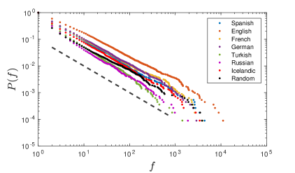
Figure 2: Cumulative of the frequency distribution $P(f)\equiv\int_{f}^{\infty}p(\zeta)d\zeta$ for single randomly chosen texts in each language: Spanish, English, French, German, Turkish, Russian, and Icelandic (colored symbols). Black dots represent a random text, and the dashed line corresponds to the expected behavior when the exponent in Zipf’s law is $\alpha=1$.

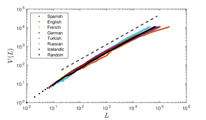
Figure 3: The Herdan-Heap’s Law $V(L)\sim L^{\beta}$ for single randomly chosen texts in each language: English, Russian, French, German, Spanish, Icelandic and Turkish. Black dots represent random texts. The dashed line corresponds to a power law with exponent $\beta=0.8$, which is the average over all the texts we studied.

Figure (3) shows the size of the vocabulary $V(L)$, as a function of the length $L$ of the text considered. Once again, all the texts, including the random texts, follow the Heaps-Herdan law $V(L)\sim L^{\beta}$ reasonably well. Again, the parameters describing the various texts are given in Appendix(A)

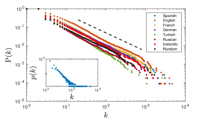
Figure 4: Cumulative of the degree distribution $\mathrm{P}(f)\equiv\int_{f}^{\infty}\mathrm{p}(\zeta)d\zeta$ for single randomly chosen texts in each language: Spanish, English, French, German, Turkish, Russian, and Icelandic (colored symbols). As in figure 2, black dots represent a random text, and the dashed line corresponds to the behavior when the exponent in Zipf’s law is $\alpha=1$. Inset: Degree distribution of the Don Quixote in French, note that the first few odd degrees $k=1,3,5,7$ deviate from the power law behavior.

Continuing with the universal laws describing texts, in figure (4) we show an example of the degree distribution for the adjacency network of the texts studied in this work. It is clear that except for the low odd degrees ($k=1,3,5,7$, see inset in fig.(4)), the distribution is well described by a power law. The parameters corresponding to the texts are given in Appendix(A). As mentioned previously, this asymptotic behavior is a consequence of Zipf’s law. If we assume that each time a word appears, the input degree $k_{in}$ (alternatively, the output degree $k_{out}$) of the corresponding node increases approximately by one, then the input degree could be expected to grow proportional to the frequency of each word. Further, in general we can expect that the total degree of a node to be $k\approx k_{in}+k_{out}\approx 2k_{in}$ (clearly this is not always true: for example, a word can appear twice, being preceded both times by the same word and followed by different words each time, leading to a degree $k=3$). Then, up to multiplicative factors, we can apply the same argument as in Equation 1 for $\mathrm{p}(k)$, the degree distribution of the network, instead of $p(f)$ From this equation it again follows that if $f(n)\sim 1/n^{\alpha}$, then $\mathrm{p}(k)\sim 1/k^{1+1/\alpha}$, which is again in close agreement with what we observe.

3 Clustering coefficient

Thus far, our results confirm that the all our texts exhibit the expected universal statistics observed in natural languages. Actually, it could be argued that these laws may be "too universal", not being able to clearly distinguish texts written in real languages from our random texts. Further, all these laws appear to be consequence of Zipf’s law, and this law reflects only the frequency of words, not their order. Thus, all three laws would still hold if the words of the texts were randomly shuffled. Clearly, shuffling the words destroys whatever relations may exist between successive words in a text, depending on the language in which it was written. This relation between successive words is what conveys meaning to a text. Thus, we expect that the clustering coefficient [27] of the adjacency network of each text,(constructed using words as nodes and linking those that are adjacent in the text), which depends strongly on the local structure, will distinguish between random texts and real texts, and even between texts in different languages.

The clustering coefficient $C_{i}(k_{i})$ of node $i$ with degree $k_{i}$ is defined as the ratio of the number of links between node $i$’s neighbors over the total number of links that would be possible for this node $k_{i}(k_{i}-1)/2$. Thus, clearly, $0\leq C_{i}(k_{i})\leq 1$. Hapax legomena, for example, mostly correspond to nodes with degree $k=2$, thus their clustering coefficient can only take the values 0 and 1 (degree $k=1$ is possible if the hapax appears followed and preceded by the same word, but these are rare occurrences). In general terms, the actual values of the clustering coefficients vary as a function of the size of the network [31], thus, in order to compare the clustering coefficients of networks corresponding to different texts, we have trimmed our texts so they all have approximately the same vocabulary size ($\simeq 11260$). In figure (5) we show an example of the clustering coefficient as a function of $k$. There are many values $C(k)$ for each $k$ corresponding to the diverse nodes with the same degree. The red points in the graph denote the average clustering coefficient for each $k$, and the solid black line is the log-binning of this average.

Figure 5: Clustering coefficient as function of the degree for Don Quixote (Spanish). The gray dots represents the $C(k)$ for each node. Red circles are the average of $C(k)$. The black line is the logarithmic binning of the average.

4 Language differentiation

In order to quantify differences between languages, for each text we define the quantity $\nu(C)$ as

$$\nu(C)=\frac{\text{Number of nodes with same $C$ value }}{\text{Vocabulary}}$$ (2)

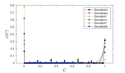
Figure 6: Fraction of nodes with same Clustering Coefficient for Don Quixote in English, Spanish, Turkish, Russian, French and German. Note that nodes with $C=0\text{ and }1$ present the largest variability between different languages

In figure (6) we show $\nu(C)$ vs $C$ for Don Quixote in six different languages. From the graph it is clear that $\nu(0)$ and $\nu(1)$ show the largest degree of variation between the various languages, thus, we propose to focus on these two numbers to characterize the various languages.

In figure (7) we show a scatter plot of $\nu(1)$ vs $\nu(0)$ for the texts in every language presented here. Using maximum likelihood estimators, we fit correlated bi-variate Gaussian distributions to the scatter plots of each language, the contour plots of which are also shown in the graph. First and most importantly, we can see in the figure that there is a clear distinction between languages and random texts. Also, we can see that languages tend to cluster in a way that is consistent with the known relationships among the languages. For example, in the figure we note that the contours corresponding to French and Spanish show a strong overlap, which might have been expected as they are closely related languages [36]. On the other hand, Russian is far from French and Spanish. This suggest that these curves may be used as a quantitative aid for the classification of languages into families. For example, French and Spanish which are both Romance languages, appear closer to each other than to Russian and Turkish, which have different origins.

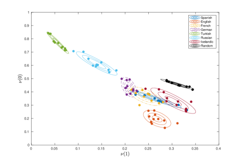
Figure 7: Bi-variate normal distribution for $\nu(0)$ and $\nu(1)$ for the different texts and random sequences. Note that differences in the distributions are clear for languages that are known to be part of different linguistic families, for example Turkish and English. Languages that belongs to the same family (Spanish and French) are essentially indistinguishable.

In order to test the validity our results, we calculate $\nu(0)$ and $\nu(1)$ for another set of books, (see tables in the appendix (B)) and using the fitted Gaussian distributions for each language, we calculated the probability that a text in each language would have those values, which allows us to assign a likelihood that a text is written in one or another language.

Books	Spanish	English	French	German	Turkish	Russian	Icelandic	Random
MobyDick(es)	10.572	0.00014223	125.25	9.1582	0	0.19125	4.0324	0
TwentyThousand…(es)	250.58	0.0033275	182.17	34.068	0	0.019141	0.45346	0
TwentyYearsLater(en)	0	230.94	0.013046	0	0	0	1.179e-07	0
BramStoker(en)	0	65.208	0.036547	0	0	0	0.00013916	0
Voltaire(fr)	266.07	0.003546	196.17	11.899	0	0.022266	0.91734	0
Miserables(fr)	23.99	0.00077475	127.1	0.0030604	0	0.02086	21.05	0
MobyDick(de)	0.026313	7.5812e-07	31.707	325.5	0	2.6555	0.8309	0
Dostoevsky(de)	0.0023808	0.00076044	4.8089	6.3034	0	2.4945e-07	1.9212e-06	0
MobyDick(tr)	0	0	0	0	977.45	2.4039	0	0
JulesVerne(tr)	0	0	0	0	25.009	0.77189	0	0
AroundWorld…(ru)	0	0	0	0	0.0098057	53.27	0	0
MysteriousIsland(ru)	0	0	0	0	5.7008	13.406	0	0
Smásögur I(is)	0	0	0.022572	0	0	0	15.199	0
Smásögur II(is)	0	0	0.58821	0	0	4.4908e-05	23.281	0
RandomTextA	0	0	0	0	0	0	4.7682e-07	5.8013
RandomTextB	0	0	0	0	0	0	0	0.045203

Table 2: Probability density function for different texts written in several languages, and random texts. Values less than $1\times 10^{-8}$ are neglected.

In table 2 we can see, for example, that it is most likely that Smásögur I (Short stories in Icelandic) are written in Icelandic than in any of the languages analyzed, or that they are a random text.

Not surprisingly, it is not so easy to tell if Voltaire in French, is really written in French or in Spanish, likewise, it is not easy to tell if Moby Dick in Spanish is written in Spanish or French, and in both cases the maximum likelihood prediction fails. Nevertheless, it is clear that these books are not written in any of the other languages presented here, nor do they correspond to a random text. On the other hand, Twenty thousand leagues under the sea in Spanish and Les Miserables in French, are correctly identified, as well as all the other texts analyzed, including the random texts.

To try to pinpoint the origin of the differentiation between different languages, we note that an inspection of the nodes with $C=0$ and $1$ reveals that they mainly consist of hapax legomena (as noted before, hapax legomena only have $C$ values of $0$ and $1$). To measure the relative importance of these words, we calculate the ratio of hapax legomena to the total number of words with $C=0$ and $1$, we call this number $\nu^{\prime}_{H}(C)$.

BookName	$\nu^{\prime}_{H}(0)$	$\nu^{\prime}_{H}(1)$
Don Quixote	0.92524	0.81389
The Count of Montecristo	0.91299	0.87284
The Three Musketeers	0.9087	0.85338
Jane Austen	0.93604	0.80736
Celebrated Crimes	0.91249	0.85042
Les Miserables	0.91795	0.87119
Anna Karenina	0.91475	0.83565
War And Peace	0.91263	0.8445
Brothers Karamazov	0.9144	0.82616
Oscar Wilde	0.85503	0.85562
Charles Dickens	0.91206	0.85831
Twenty Years Later	0.92125	0.84953
Bram Stoker	0.92612	0.84925

Table 3: Fraction of hapax legomena with clustering coefficient equal to $0$ or $1$ for English texts

In Table 3, we show the fraction of hapax legomena of the words with $C=0,1$ for several texts in English. A value close to $1$ indicates that most of the nodes that contribute to $\nu^{\prime}_{H}(C)$ are words that appear only once in the document. This indicates that the local structure around those words, i.e, the way that they relate in the adjacency network, is particular to each language, and seems to be a key for language differentiation.

Language	$\overline{\nu^{\prime}_{H}(0)}$	$\overline{\nu^{\prime}_{H}(1)}$
Spanish	0.9002	0.9146
English	0.9131	0.8452
French	0.9023	0.9287
German	0.9008	0.9440
Turkish	0.8079	0.9797
Russian	0.8676	0.9618
Icelandic	0.9148	0.8980
Random	0.9600	0.9637

Table 4: Average values of $\nu^{\prime}_{H}(C)$ for Spanish, English, French, German, Turkish, Icelandic and Random texts.

In the Table 4 we see the average of $\nu^{\prime}_{H}(C)$ for each of the languages studied here. Note that for example the values are clearly different for Spanish and Turkish, similar for Spanish and French, and very different for all languages and random.

5 Conclusions

Zipf’s law is one of the most universal statistics of natural languages. However, it may be too universal. While it may not strictly apply to sequences of independent random symbols with random spacings [33], it appears to describe random texts that conserve most of the correlations between successive symbols, as accurately as it describes texts written in real languages. Further, Heaps-Herdan law and the degree distribution of the adjacency network, appear to be consequences of Zipf’s law, and are, thus, as universal.

In this work we studied 91 texts in seven different languages, as well as random texts constructed by randomizing the spacings between words without altering the order of the letters in the text. We find that they are all well described by the universal laws. However, we also found that the distribution of clustering coefficients of the networks of each text appears to vary from one language to another, and to distinguish random texts from real languages. The nodes that vary the most among the distributions of $C(k)$ are those for which $C(k)$ is equal to $0$ or $1$. We fit the scatter plot of these nodes to bivariate Gaussian distributions, which allows us to define the likelihood that a text is written in each given language. This method was very successful identifying the languages in which test were written, only failing to distinguish a couple of texts, confusing texts french and spanish, which have a strong overlap. In Table (2) we present the evidence that we can use the statistics of clustering coefficient to measure a sort of distance between languages.

Though hapax legomena account for most of the value $\nu(C)$ for $C=0$ and 1, we found that the fraction $\nu^{\prime}_{H}(C)$ of hapax to other words is similar for French and Spanish, and different for Spanish and, say, Turkish. Further, $\nu^{\prime}_{H}(C)$ is different between random texts and the languages we study. These observations might give some clue to the mechanism by which the clustering coefficient, and in particular the local structure around hapax legomena, helps to differentiate languages.

Unlike the work presented by Gamallo et. al [28], which is Corpus-based, our work uses a relatively small amount of texts. Also as we can see in tables presented in Appendix (A), the length of the texts we use is not necessarily the length of the complete work. Texts were cut at the appropriate length for all of them to have approximately the same vocabulary ($\simeq 11260$). Thus, actual lengths ranged from $368076$ words for the Jane Austen books in English, to $26347$ words for the text we called Turkish I. This is important not only for computational reasons, it may also be important for studies of the relation between languages for which large corpora do not exist, something very common in the linguistic studies of the indigenous languages. The method proposed in this work can be useful in such cases, as small texts trimmed to fill some appropriate vocabulary size is the only necessary ingredient.

6 Acknowledgments

Diego Espitia acknowledges financial support through a doctoral scholarship from Consejo Nacional de Ciencia y Tecnología (CONACyT).

Appendix A Tables and Results

In this appendix we present tables of results for the data analyzed in this work. Here $\alpha_{k}$ and $\sigma_{k}$ represent the exponent and standard error of the power law for the degree distribution of the co-occurrence networks $p(k)\propto 1/k^{\alpha_{k}}$, for $k>k_{min}$, where $k_{min}$ is the smallest degree for which the power law holds. Similarly, $\alpha_{Z}$ and $\sigma_{z}$ represents the exponent and standard error of the distribution of frequencies $p(f)\propto 1/f^{\alpha_{z}}$; for $f>f_{min}$ where now $f_{min}$ is the smallest frequency for which the power law is satisfied. The values of the Heap’s law $\beta$ and $\sigma_{h}$ were obtained via least square fitting.

For the estimation of the parameters we use the Maximum Likelihood Estimation (MLE) method for discerning and quantifying power-law behavior in empirical data [37]. The MLE works as follows: assuming that the data fits a power law, we estimate $\alpha$ via

$$\hat{\alpha}^{*}=1+N\left[\sum_{i=1}^{N}\ln\frac{x_{i}}{x^{*}_{min}-\frac{1}{2}}\right]^{-1},$$ (3)

where $x_{i}>x_{min}^{*}$ for $i=1,...N$ and using as $x^{*}_{min}$ each element of the data set $\{x\}$. Then, using the Kolmogorov–Smirnov test we find the distance $D$ between the cumulative distribution of the data set and the cumulative distribution $P_{(x^{*}_{min},\alpha^{*})}(x)$. From these set of distances, we find the value which minimizes $D$, this $x_{min}$, is the smallest data for which the power law holds, and can be used to determine the parameter of the power law $\hat{\alpha}$. In order to perform a goodness of the fit test, we construct $1000$ synthetic data, using the previous $\hat{\alpha}$ and $x_{min}$. Now we can count the fraction of the synthetic distances that are larger than the distance obtained from the data. This fraction is known as p-value If this p-value$>0.1$, then the difference between the data set and the model can be attributed to statistical fluctuations alone; if it is small, the model is not a plausible fit to the data.[37]

Spanish

Book Name	Length	Vocabulary	$\alpha_{k}$	$\sigma_{k}$	$k_{min}$	p-value	$\alpha_{Z}$	$\sigma_{Z}$	$f_{min}$	p-value	$\beta$	$\sigma_{h}$
The Count of Montecristo	92378	11275	2.15	0.03	9	0.439	1.87	0.01	1	0.640	0.781	0.002
Don Quixote	113068	11277	2.11	0.03	10	0.206	1.84	0.01	1	0.119	0.810	0.002
The Three Musketeers	106869	11242	2.10	0.03	11	0.669	1.86	0.01	1	0.203	0.746	0.002
Unamuno	104769	11219	2.05	0.03	10	0.602	1.89	0.01	1	0.107	0.765	0.002
Valle-Inclan	76657	11252	2.24	0.03	8	0.532	2.04	0.02	5	0.331	0.780	0.002
Concha Espina	60356	11226	2.33	0.04	9	0.190	2.12	0.03	4	0.445	0.814	0.001
Angelina	71434	11281	2.23	0.03	8	0.180	2.02	0.02	3	0.583	0.810	0.002
Iliad	91203	11275	2.19	0.03	8	0.658	1.96	0.02	4	0.419	0.799	0.002
Odyssey	92381	11290	2.18	0.02	6	0.289	1.96	0.02	4	0.510	0.797	0.002
Pio Baroja	85227	11273	2.21	0.03	8	0.601	2.03	0.03	7	0.362	0.787	0.001
The White Company	76186	11232	2.18	0.03	9	0.126	1.97	0.02	3	0.510	0.786	0.002
Moby Dick	69986	11230	2.15	0.03	9	0.249	2.00	0.01	2	0.533	0.795	0.002
TwentyThousand	76443	11214	2.22	0.03	9	0.105	2.01	0.02	3	0.860	0.788	0.001

English

BookName	Length	Vocabulary	$\alpha_{k}$	$\sigma_{k}$	$k_{min}$	p-value	$\alpha_{Z}$	$\sigma_{Z}$	$f_{min}$	p-value	$\beta$	$\sigma_{h}$
Don Quixote	221474	11278	2.16	0.03	17	0.417	1.90	0.02	15	0.823	0.731	0.003
The Count of Montecristo	178516	11261	2.17	0.03	19	0.244	1.97	0.03	16	0.934	0.703	0.002
The Three Musketeers	233220	11266	2.14	0.03	24	0.972	1.91	0.03	33	0.579	0.704	0.003
Jane Austen	368076	11270	2.16	0.03	34	0.805	1.93	0.04	84	0.702	0.660	0.003
Celebrated Crimes	156044	11274	2.20	0.03	17	0.569	2.05	0.04	28	0.505	0.726	0.002
Les Miserables	131649	11254	2.17	0.04	19	0.198	1.97	0.03	10	0.867	0.736	0.002
Anna Karenina	259749	11268	2.13	0.03	20	0.965	1.86	0.02	11	0.105	0.687	0.002
War And Peace	201580	11223	2.17	0.04	33	0.612	1.94	0.03	25	0.590	0.699	0.002
Brothers Karamazov	291642	11212	2.12	0.03	27	0.647	1.85	0.02	22	0.600	0.686	0.003
Oscar Wilde	174912	11262	2.15	0.04	28	0.865	1.92	0.03	24	0.774	0.716	0.002
Charles Dickens	183844	11266	2.12	0.03	20	0.738	1.89	0.02	9	0.992	0.714	0.002
Twenty Years Later	231543	11257	2.12	0.04	29	0.854	1.92	0.04	44	0.718	0.701	0.003
Bram Stoker	221752	11265	2.13	0.03	23	0.182	1.88	0.03	20	0.804	0.691	0.002

French

Book Name	Length	Vocabulary	$\alpha_{k}$	$\sigma_{k}$	$k_{min}$	p-value	$\alpha_{Z}$	$\sigma_{Z}$	$f_{min}$	p-value	$\beta$	$\sigma_{h}$
The Count of Montecristo	105525	11271	2.10	0.03	9	0.378	1.89	0.02	3	0.681	0.745	0.002
Don Quixote	111728	11237	2.10	0.02	8	0.495	1.89	0.02	5	0.628	0.746	0.002
The Three Musketeers	111274	11268	2.07	0.03	11	0.520	1.85	0.01	1	0.326	0.768	0.002
Oscar Wilde	85015	11206	2.15	0.03	8	0.422	1.92	0.01	1	0.538	0.783	0.002
Madame Bobary	72966	11292	2.22	0.03	8	0.001	2.00	0.01	2	0.940	0.782	0.002
Honoré de Balzac	78495	11264	2.17	0.03	9	0.062	1.98	0.02	3	0.160	0.799	0.002
Homero	149951	11236	2.11	0.03	11	0.682	1.86	0.02	7	0.212	0.722	0.002
Notre Dame	69988	11282	2.18	0.03	9	0.012	1.98	0.01	1	0.965	0.784	0.001
Lesuieur	85886	11250	2.17	0.03	8	0.122	1.97	0.02	4	0.729	0.778	0.002
Guy de Maupassant	74709	11257	2.16	0.03	9	0.068	1.93	0.01	1	0.499	0.795	0.002
Twenty Thousand Leagues Under the Sea	74369	11272	2.23	0.03	8	0.001	2.00	0.02	3	0.895	0.781	0.002
Voltaire	81450	11267	2.15	0.03	9	0.002	1.95	0.01	2	0.160	0.772	0.001
Les Miserables	79011	11275	2.14	0.03	9	0.238	1.95	0.01	1	0.769	0.784	0.001

German

Book Name	Length	Vocabulary	$\alpha_{k}$	$\sigma_{k}$	$k_{min}$	p-value	$\alpha_{Z}$	$\sigma_{Z}$	$f_{min}$	p-value	$\beta$	$\sigma_{h}$
The Count of Montecristo	99693	11263	2.06	0.02	8	0.669	1.82	0.01	1	0.156	0.738	0.002
Don Quixote	81741	11323	2.07	0.03	10	0.716	1.92	0.01	1	0.385	0.921	0.006
The Three Musketeers	107870	11271	2.04	0.03	13	0.623	1.82	0.01	1	0.629	0.743	0.002
Honoré de Balzac	75986	11287	2.05	0.03	11	0.414	1.93	0.01	1	0.772	0.783	0.002
Rudolf Hans Bartsch	58874	11288	2.07	0.04	18	0.496	1.94	0.03	5	0.705	0.805	0.002
Felix Dahn I	67330	11268	2.17	0.05	23	0.616	1.96	0.01	1	0.404	0.785	0.002
Felix Dahn II	75792	11257	2.09	0.02	8	0.658	1.91	0.01	1	0.248	0.781	0.002
Charles Dickens I	82374	11274	2.06	0.02	8	0.128	1.90	0.01	1	0.853	0.779	0.002
Cahrles Dickens II	81893	11285	2.00	0.03	9	0.256	1.92	0.01	1	0.536	0.822	0.003
Alfred Döblin	56757	11240	2.12	0.03	10	0.595	2.02	0.02	2	0.526	0.787	0.002
Gustave Falke	62815	11202	2.07	0.03	10	0.939	1.96	0.02	3	0.225	0.788	0.002
MobyDick	72414	11215	2.08	0.03	12	0.676	1.94	0.01	2	0.329	0.779	0.002
Crime and Punishment	96492	11260	2.19	0.05	28	0.366	1.80	0.01	1	0.879	0.756	0.002

Turkish

BookName	Length	Vocabulary	$\alpha_{k}$	$\sigma_{k}$	$k_{min}$	p-value	$\alpha_{Z}$	$\sigma_{Z}$	$f_{min}$	p-value	$\beta$	$\sigma_{h}$
The Count of Montecristo	42040	11198	2.26	0.06	19	0.524	2.07	0.02	2	0.455	0.822	0.001
Don Quixote	35207	11241	2.27	0.05	12	0.162	2.18	0.01	1	0.310	0.881	0.002
The Three Musketeers	40731	11280	2.22	0.04	10	0.145	2.07	0.02	2	0.317	0.857	0.002
Tale of Two Cities	37838	11292	2.26	0.04	11	0.371	2.14	0.01	1	0.113	0.855	0.002
Oscar Wilde	35065	11205	2.29	0.05	14	0.182	2.13	0.02	2	0.367	0.866	0.002
Jules Verne I	35595	11264	2.29	0.05	12	0.713	2.11	0.02	2	0.592	0.845	0.001
David Copperfield	39672	11213	2.23	0.04	10	0.711	2.09	0.02	2	0.595	0.854	0.002
Crime and Punishment	39716	11279	2.25	0.04	12	0.197	2.10	0.01	1	0.756	0.855	0.002
Turkish I	26347	11240	2.50	0.08	16	0.944	2.34	0.01	1	0.357	0.913	0.001
Turkish II	26765	11244	2.43	0.07	14	0.934	2.31	0.02	2	0.204	0.904	0.002
Turkish III	27564	11288	2.34	0.06	12	0.487	2.21	0.04	4	0.336	0.883	0.001
MobyDick	33500	11224	2.31	0.06	16	0.352	2.19	0.01	1	0.455	0.881	0.001
Jules Verne II	40060	11225	2.25	0.04	10	0.386	2.06	0.01	1	0.189	0.863	0.002

Russian

Book Name	Length	Vocabulary	$\alpha_{k}$	$\sigma_{k}$	$k_{min}$	p-value	$\alpha_{Z}$	$\sigma_{Z}$	$f_{min}$	p-value	$\beta$	$\sigma_{h}$
Don Quixote	41169	11277	2.16	0.04	10	0.799	2.21	0.01	1	0.485	0.864	0.002
The Count of Montecristo	47282	11234	2.16	0.04	10	0.615	2.11	0.01	1	0.367	0.802	0.002
The Three Musketeers	51306	11277	2.14	0.03	10	0.869	2.06	0.01	1	0.196	0.818	0.002
Anna Karenina	53333	11242	2.12	0.04	11	0.625	2.02	0.02	2	0.175	0.823	0.002
War And Peace	45596	11321	2.14	0.03	9	0.019	2.09	0.01	1	0.232	0.821	0.002
Brothers Karamazov	47083	11293	2.11	0.05	16	0.861	2.16	0.01	1	0.785	0.835	0.002
Twenty Thousand Leagues Under the Sea	35961	11297	2.29	0.05	10	0.766	2.21	0.01	1	0.108	0.865	0.002
Anton Chekhov	45423	11282	2.18	0.04	11	0.713	2.13	0.01	1	0.714	0.869	0.002
Oscar Wilde	43504	11321	2.10	0.04	12	0.792	2.00	0.04	7	0.624	0.823	0.002
Honoré de Balzac	35407	11280	2.15	0.05	12	0.886	2.05	0.04	5	0.429	0.881	0.002
Twenty Years Later	48539	11250	2.10	0.04	11	0.636	1.99	0.03	4	0.801	0.823	0.002
Moby Dick	34748	11234	2.16	0.05	11	0.578	2.07	0.03	4	0.856	0.857	0.002
Crime and Punishment	40035	11217	2.19	0.05	16	0.724	2.15	0.01	1	0.678	0.835	0.001

Icelandic

BookName	Length	Vocabulary	$\alpha_{k}$	$\sigma_{k}$	$k_{min}$	p-value	$\alpha_{Z}$	$\sigma_{Z}$	$f_{min}$	p-value	$\beta$	$\sigma_{h}$
TorfhildiHólm	73242	11202	2.18	0.06	29	0.838	1.97	0.01	1	0.156	0.773	0.002
SagaI	99051	11184	2.03	0.02	8	0.148	1.88	0.01	1	0.569	0.753	0.001
SagaII	141436	11248	1.95	0.02	6	0.501	1.76	0.01	1	0.551	0.714	0.002
SagaIII	103020	11270	2.00	0.02	8	0.964	1.84	0.01	2	0.640	0.734	0.001
SagaIV	116521	11235	1.99	0.02	6	0.256	1.81	0.01	1	0.102	0.735	0.002
SagaV	106061	11290	1.98	0.02	6	0.465	1.84	0.01	1	0.659	0.729	0.001
SagaVI	116956	11296	2.21	0.06	50	0.634	1.83	0.01	1	0.118	0.734	0.002
SagaVII	119928	11287	2.20	0.06	49	0.794	1.81	0.01	1	0.216	0.742	0.001
JónTrausti	66577	11238	2.05	0.03	9	0.278	1.94	0.02	3	0.553	0.785	0.001
JónThoroddsen	89739	11249	2.02	0.03	8	0.148	1.85	0.02	4	0.273	0.757	0.001
ÞorgilsGjallanda	65357	11285	2.10	0.03	8	0.227	1.97	0.02	2	0.295	0.786	0.001
SmásögurI	58932	11287	2.10	0.03	9	0.717	1.98	0.02	4	0.811	0.803	0.001
SmásögurII	61272	11226	2.10	0.04	12	0.301	1.99	0.02	2	0.126	0.803	0.001

Random

Book Name	Length	Vocabulary	$\alpha_{k}$	$\sigma_{k}$	$k_{min}$	p-value	$\alpha_{Z}$	$\sigma_{Z}$	$f_{min}$	p-value	$\beta$	$\sigma_{h}$
Random I	63904	11258	2.05	0.03	10	0.901	1.88	0.02	3	0.952	0.805	0.001
Random II	62391	11251	2.00	0.04	12	0.335	1.88	0.02	3	0.678	0.788	0.001
Random III	62619	11286	2.02	0.03	9	0.522	1.90	0.02	3	0.445	0.802	0.001
Random IV	61148	11208	1.99	0.03	11	0.256	1.91	0.02	3	0.856	0.808	0.001
Random V	63181	11291	2.04	0.03	8	0.407	1.93	0.02	2	0.225	0.791	0.001
Random VI	62430	11302	2.00	0.04	14	0.294	1.87	0.03	5	0.247	0.796	0.001
Random VII	66740	11224	2.10	0.06	29	0.588	1.88	0.04	10	0.704	0.804	0.001
Random VIII	65939	11251	1.98	0.03	10	0.008	1.86	0.02	4	0.478	0.812	0.002
Random IX	62318	11247	2.03	0.03	9	0.258	1.90	0.02	3	0.151	0.810	0.001
Random X	61574	11239	1.98	0.03	11	0.395	1.92	0.02	2	0.102	0.814	0.001
Random A	66795	11277	2.01	0.03	9	0.812	1.87	0.03	5	0.523	0.797	0.001
Random B	65996	11262	2.01	0.04	11	0.895	1.88	0.03	4	0.755	0.797	0.001

Appendix B Texts used

Here we present the text used in this work. The vast majority of the texts were obtained from the Gutemberg project, except for the texts in Russian, Turkish and Icelandic, which were obtained from other sources.

Spanish
Alexandre Dumas	The Count of Montecristo The Three Musketeers
Miguel de Cervantes	Don Quixote
Miguel de Unamuno	Niebla Una Historia De Pasión
Ramón del Valle-Inclan	Memorias Del Marqués De Bradomin: Sonata De Otoño Sonata De Verano Sonata De Primavera Sonata De Invierno
Concha Espina	Agua De Nieve La Esfinge Maragata Dulce Nombre
Rafael Delgado	Angelina
Homer	Iliad Odyssey
Pío Baroja	Memorias De Un Hombre De Acción: El Aprendiz De Conspirador Los Caminos Del Mundo
Arthur Conan Doyle	The White Company
Herman Melville	Moby Dick
Jules Verne	Twenty Thousand Leagues Under the Sea

Table 5: Source: Gutemberg Project

English
Miguel de Cervantes	Don Quixote
Alexandre Dumas	The Count of Montecristo The Three Musketeers Celebrated Crimes Twenty Years Later
Jane Austen	Mansfield Park Northanger Abbey Persuasion Sense and Sensibility
Victor Hugo	Les Miserables
Leon Tolstói	Anna Karenina War and Peace
Fyodor Dostoevsky	Brothers Karamazov
Oscar Wilde	The Picture of Dorian Gray The Happy Prince and Other Tales De Profundis A House Of Pomegranates The Canterville Ghost Selected Prose Of Oscar Wilde
Charles Dickens	Oliver Twist A Tale Of Two Cities
Bram Stoker	Dracula The Jewel of Seven Stars

Table 6: Source: Gutemberg Project

Turkish
Alexandre Dumas	The Count of Montecristo The Three Musketeers
Miguel de Cervantes	Don Quixote
Charles Dickens	A Tale of Two Cities David Copperfield
Turkish I Turkish II Turkish III	Modern prose: samples from literary texts and newspapers
Jules Verne	Twenty Thousand Leagues Under the Sea From the Earth to the Moon Around the World in 80 Days
Herman Melville	Moby Dick
Fyodor Dostoevsky	Crime and Punishment

Table 7: Source: www.ekitapcilar.com.
Turkish I, II and III were obtained from
University of Oxford Text Archive
(http://ota.ox.ac.uk/desc/0387)

Russian
Alexandre Dumas	The Count of Montecristo The Three Musketeers Twenty Years Later
Miguel de Cervantes	Don Quixote
Oscar Wilde	The Portrait of Dorian Gray De Profundis
Honoré de Balzac	Fater Goriot A Woman of Thirty
Jules Verne	Twenty Thousand Leagues Under the Sea Mysterious Island Around the World in 80 Days
Anton Chekhov	Short Stories Compilation
Fyodor Dostoevsky	Brothers Karamazov
Leo Tolstoy	Anna Karenina War And Peace

Table 8: Source: https://www.e-reading.club

French
Miguel de Cervantes	Don Quixote
Alexandre Dumas	The Count of Montecristo The Three Musketeers
Victor Hugo	The Hunchback of Notre-Dame Les Miserables
Jules Verne	Twenty Thousand Leagues Under the Sea
Guy de Maupassant	Ball of Fat Moonlight Contes de la Bécasse
Oscar Wilde	The Portrait of Dorian Gray Intentions
Gustave Flaubert	Madame Bovary
Honoré de Balzac	The Human Comedy. Scenes from private life: At the Sign of the Cat and Racket The Ball at Sceaux The Purse The Vendetta Madame Firmiani A Second Home Domestic Bliss The Imaginary Mistress Study of a Woman Albert Savarus
Homer	Iliad
Daniel Lesueur (Jeanne Lapauze)	Amour D’Aujourd’Hui
Voltaire	Candide

Table 9: Source: Gutemberg Project

German
Alexandre Dumas	The Count of Montecristo The Three Musketeers
Miguel de Cervantes	Don Quixote
Honoré de Balzac	Grosse Und Kleine Welt (Short Stories) A Woman of Thirty
Rudolf Hans Bartsch	Grenzen der Menschheit Vom sterbenden Rokoko
Felix Dahn	Ein Kampf um Rom I Ein Kampf um Rom II
Charles Dickens	Oliver Twist A Tale of Two Cities
Alfred Döblin	Die Lobensteiner reisen nach Böhmen
Gustav Falke	Der Mann im Nebel
Herman Melville	Moby Dick
Fyodor Dostoevsky	Crime and Punishment

Table 10: Source: Gutemberg Project

Table 11: Source: All sagas were obtained from https://sagadb.org/. The other texts were obtained from https://www.snerpa.is/net/index.html

Icelandic
Torfhildi Hólm	Brynjólfur Biskup Sveinsson
Sagas I	Bandamanna Saga Bardar Saga Bjarnar Saga Droplaugarsona Saga Gisla Saga Hrafnkels Saga Eiríks Saga Eyrbyggja Saga
Sagas II	Brennu-Njáls Saga Laxdæla Saga
Sagas III	Egils Saga Grettis Saga
Sagas IV	Finnboga Saga Fljótsdæla Saga Flóamanna Saga Fóstbræðra Saga Grænlendinga Saga Gull-Þóris Saga
Sagas V	Gunnars Saga Gunnlaugs Saga Hænsna-Þóris Saga Hallfreðar Saga Harðar Saga Hávarðar Saga Heiðarvíga Saga Hrana Saga
Sagas VI	Kjalnesinga Saga Kormáks Saga Króka-Refs Saga Ljósvetninga Saga Reykdæla Saga Svarfdæla Saga Þórðar Saga
Sagas VII	Þorsteins Saga Hvíta Þorsteins Saga Síðu-Hallssonar Valla-Ljóts Saga Vatnsdæla Saga Víga-Glúms Saga Víglundar Saga Vopnfirðinga Saga Færeyinga Saga Ölkofra Saga Laxdæla Saga
Jón Trausti	Anna Frá Stóruborg Borgir
Jón Thoroddsen	Maður Og Kona
Þorgils Gjallanda	Upp Við Fossa Gamalt Og Nýtt
Smásögur I	Brúðardraugurinn Írafells - Móri Sagan Af Heljarslóðarorrustu Ferðasaga Þórðar Saga Geirmundarsonar Grímur Kaupmaður Deyr Hans Vöggur
Smásögur II	Kærleiksheimilið Brennivínshatturinn Gulrætur Í vinnunni Einræða Vordraumur Kvöld, nótt, morgunn

References

[1]
George Zipf.
Human behavior and the principle of least effort: an
introduction to human ecology.
Addison-Wesley Press, Cambridge, MA, 1st edition, 1949.
[2]
Murray Gell Mann and Merritt Ruhlen.
The origin and evolution of word order.
Proceedings of the National Academy of Sciences of the United
States of America, 108:17290–5, 10 2011.
[3]
I. Kontoyiannis, P. H. Algoet, Y. M. Suhov, and A. J. Wyner.
Nonparametric entropy estimation for stationary processes and random
fields, with applications to english text.
IEEE Transactions on Information Theory, 44(3):1319–1327, May
1998.
[4]
Reinhard Köhler.
Syntactic structures: Properties and interrelations.
Journal of Quantitative Linguistics, 6(1):46–57, 1999.
[5]
D. H. Zanette.
Statistical patterns in written language.
arXiv:1412.3336, 2014.
[6]
Eduardo Altmann and Martin Gerlach.
Statistical laws in linguistics.
arXiv: 1502.03296, 02 2015.
[7]
Kevin Knight Sravana Reddy.
What we know about the voynich manuscript.
Proceedings of the 5th ACL-HLT Workshop on Language Technology
for Cultural Heritage, Social Sciences, and Humanities, page 78–86, 2011.
[8]
Diego R. Amancio, Eduardo G. Altmann, Diego Rybski, Osvaldo N. Oliveira, Jr,
and Luciano da F. Costa.
Probing the statistical properties of unknown texts: Application to
the voynich manuscript.
PLOS ONE, 8(7):1–10, 07 2013.
[9]
Marcelo A. Montemurro and Damián H. Zanette.
Keywords and co-occurrence patterns in the voynich manuscript: An
information-theoretic analysis.
PLOS ONE, 8(6):1–9, 06 2013.
[10]
Kevin Knight, Beáta Megyesi, and Christiane Schaefer.
The secrets of the copiale cipher.
Journal for Research into Freemasonry and Fraternalism, 05
2012.
[11]
Kevin Knight, Beáta Megyesi, and Christiane Schaefer.
The copiale cipher.
In Proceedings of the 4th Workshop on Building and Using
Comparable Corpora: Comparable Corpora and the Web, pages 2–9, Portland,
Oregon, June 2011. Association for Computational Linguistics.
[12]
Steven T. Piantadosi.
Zipf’s word frequency law in natural language: A critical review and
future directions.
Psychonomic Bulletin & Review, 21(5):1112–1130, Oct 2014.
[13]
Jake Ryland Williams, Paul R. Lessard, Suma Desu, Eric M. Clark, James P.
Bagrow, Christopher M. Danforth, and Peter Sheridan Dodds.
Zipf’s law holds for phrases, not words.
Scientific Reports, 5:12209 EP –, Aug 2015.
Article.
[14]
Isabel Moreno-Sánchez, Francesc Font-Clos, and Álvaro Corral.
Large-scale analysis of zipf’s law in english texts.
PLOS ONE, 11(1):1–19, 01 2016.
[15]
Mark Newman.
The power of design.
Nature, 405(6785):412–413, 2000.
[16]
R. Ferrer i Cancho.
The variation of zipf’s law in human language.
The European Physical Journal B - Condensed Matter and Complex
Systems, 44(2):249–257, Mar 2005.
[17]
Peter Zörnig.
Zipf’s law for randomly generated frequencies: explicit tests for the
goodness-of-fit.
Journal of Statistical Computation and Simulation,
85(11):2202–2213, 2015.
[18]
W. Li.
Random texts exhibit zipf’s-law-like word frequency distribution.
IEEE Transactions on Information Theory, 38(6):1842–1845, Nov
1992.
[19]
Gustav Herdan.
Type-token mathematics.
The Hague: Mouton, 1960.
[20]
Harold Stanley Heaps.
Information Retrieval: Computational and Theoretical Aspects.
Academic Press, 1978.
[21]
Ricardo Baeza-Yates and Gonzalo Navarro.
Block addressing indices for approximate text retrieval.
Proceedings of the sixth international conference on Information
and knowledge management - CIKM 97, pages 69–82, 2000.
[22]
Leo Egghe.
Untangling herdans law and heaps law: Mathematical and informetric
arguments.
Journal of the American Society for Information Science and
Technology, 58(5):702–709, 2007.
[23]
Ramon Ferrer i Cancho, Ricard V. Solé, and Reinhard Köhler.
Patterns in syntactic dependency networks.
Phys. Rev. E, 69:051915, May 2004.
[24]
Camilo Akimushkin, Diego Raphael Amancio, and Osvaldo Novais Oliveira, Jr.
Text authorship identified using the dynamics of word co-occurrence
networks.
PLOS ONE, 12(1):1–15, 01 2017.
[25]
HaiTao Liu and Jin Cong.
Language clustering with word co-occurrence networks based on
parallel texts.
Chinese Science Bulletin, 58(10):1139–1144, Apr 2013.
[26]
Y. Matsuo and M. Ishizuka.
Keyword extraction from a single document using word co-occurrence
statistical information.
International Journal on Artificial Intelligence Tools,
13(01):157–169, 2004.
[28]
Pablo Gamallo, José Ramom Pichel, and Iñaki Alegria.
From language identification to language distance.
Physica A: Statistical Mechanics and its Applications, 484:152
– 162, 2017.
[29]
Barry R. Chiswick and Paul W. Miller.
Linguistic distance: A quantitative measure of the distance between
english and other languages.
Journal of Multilingual and Multicultural Development,
26(1):1–11, 2005.
[30]
Filippo Petroni and Maurizio Serva.
Measures of lexical distance between languages.
Physica A: Statistical Mechanics and its Applications,
389(11):2280 – 2283, 2010.
[31]
Agata Fronczak, Piotr Fronczak, and Janusz A. Hołyst.
Mean-field theory for clustering coefficients in barabási-albert
networks.
Phys. Rev. E, 68:046126, Oct 2003.
[32]
George A. Miller.
Some effects of intermittent silence.
The American Journal of Psychology, 70(2):311–314, 1957.
[33]
Ramon Ferrer-i Cancho and Brita Elvevå g.
Random texts do not exhibit the real zipf’s law-like rank
distribution.
PLOS ONE, 5(3):1–10, 03 2010.
[34]
Ramon Ferrer i Cancho and Ricard V. Solé.
Two regimes in the frequency of words and the origins of complex
lexicons: Zipf’s law revisited.
Journal of Quantitative Linguistics, 8(3):165–173, 2001.
[35]
G.G. Naumis and G. Cocho.
Tail universalities in rank distributions as an algebraic problem:
The beta-like function.
Physica A: Statistical Mechanics and its Applications,
387(1):84 – 96, 2008.