CNAK : Cluster Number Assisted K-means

Abstract

Determining the number of clusters present in a dataset is an important problem in cluster analysis. Conventional clustering techniques generally assume this parameter to be provided up front. In this paper, we propose a method which analyzes cluster stability for predicting the cluster number. Under the same computational framework, the technique also finds representatives of the clusters. The method is apt for handling big data, as we design the algorithm using Monte-Carlo simulation. Also, we explore a few pertinent issues found to be of also clustering. Experiments reveal that the proposed method is capable of identifying a single cluster. It is robust in handling high dimensional dataset and performs reasonably well over datasets having cluster imbalance. Moreover, it can indicate cluster hierarchy, if present. Overall we have observed significant improvement in speed and quality for predicting cluster numbers as well as the composition of clusters in a large dataset.

1 Introduction

In cluster analysis, it is required to group a set of data points in a multi-dimensional space, so that data points in the same group are more similar to each other than to those in other groups. These groups are called clusters. Various distance functions may be used to compute the degree of similarity or dissimilarity among these data points. Typically Euclidean distance function is widely used in clustering. The aim of this unsupervised technique is to increase homogeneity in a group and heterogeneity between groups. Several clustering methods with different characteristics have been proposed for different purposes. Some well-known methods include partition-based clustering [26], hierarchical clustering [25], spectral clustering [27], density-based clustering [12]. However, they require the knowledge of cluster number for a given dataset a priori [26, 27, 12, 36, 21]. Nevertheless, the estimation of the number of clusters is a difficult problem as the underlying data distribution is unknown. Readers can find several existing techniques for determining cluster number in [19, 6]. We have followed the nomenclature used in [6] for categorizing different methods for the prediction of cluster number. In this work, we choose to focus only on three approaches: 1) Variance-based approach, 2) Structural approach, and 3) Resampling approach. Variance-based approaches are based on measuring compactness within a cluster. Structural approaches include between-cluster separation as well as within cluster variance. We have chosen these approaches as they are either more suitable for handling big data, or appear in a comparative study by several researchers. Some well known approaches are Calinski-Harabaz [3], Silhouette Coefficient [30], Davies-Bouldin [8], Jump [31], Gap statistic [32], etc. These approaches are not appropriate for handling the big data, as they are computationally intensive and require large storage space. It requires a scalable solution [13, 18] for identifying the number of clusters. Resampling-based approaches can be considered in such a scenario. Recently, the concept of stability in clustering has become popular. A few methods [14, 35] utilize the concept of clustering robustness against the randomness in the choice of sampled datasets to explore clustering stability. In the following subsection, we discuss our motivation for this work.

1.1 Motivation

In general, clustering algorithms deal with two problems: 1) estimation of natural cluster number, and 2) determination of well-organized groups. In the current scenario, many applications requiring the task of clustering target a large size of data. Therefore, a scalable solution is required for determining cluster number and well-formed groups. There are clustering methods [7], which employ Monte-Carlo based techniques to perform clustering on a large dataset. But, they require prior information about the cluster number. Also, there is no such built-in method to select the size of a sampled dataset in Monte-Carlo based methods. Existing methods usually sample a large fraction of dataset, and use them for clustering. Hence, the improvement with respect to computational time for those algorithms is limited. The objectives for this work are as follows: 1) estimation of cluster number, 2) simultaneous computation of cluster representatives during the process of estimation, and 3) estimation of the required size for a sampled dataset in Monte-Carlo Simulation. Our contributions in this work are summarized below.

• We propose a Monte-Carlo based technique to determine appropriate cluster number for a given dataset. We derive cluster representatives from the same method.

• We propose a model for estimating the size of the sampled dataset for the Monte-Carlo based simulation. Also, we test the relevance of the solution empirically with many datasets.

• We demonstrate the applicability of our proposed method for large-scale datasets.

• We explore the behavior of our method in a few relevant issues in clustering, such as 1) cluster overlapping, 2) shape clusters, and 3) clustering in the presence of noise.

2 Proposed Work

It comprises of two steps. First, it estimates the cluster number. Subsequently, it presents the clustering technique which provides support towards the correctness of cluster number prediction.

2.1 Cluster Number Prediction

We use a fraction of the original dataset to predict cluster number. Initially, we randomly select a sampled dataset of size $\frac{1}{s}$ of the original dataset. We prepare $T$ such random sampled sets. Then, we generate $k$ cluster centers by applying k-means++ [1] algorithm to each sampled datasets. Hence, we have $T$ instances of cluster centers of the original dataset. We perform a bipartite matching between each pair of $k$ centroids, generated from each pair of $T$ sampled datasets. The central idea is as follows:

If natural cluster number is chosen for clustering, then every k-means clustering on different sampled dataset should have near-by cluster centers. Hence, the average distance between matched centroids of each pair of the sampled dataset should be minimum for the true cluster number. Thus, if we plot such a distance in a normalized form against $k$ that varies from $2$ to any higher positive integer, we should get a local minimum in the plot near the true cluster number for an underlying dataset. It is recommended to take a range of cluster numbers to compute these normalized distances if any knowledge about it exists for a given dataset.

2.1.1 Problem Formulation

We have designed our problem in two steps. The first step describes one to one mapping of cluster centers from sampled dataset $X$ to sampled dataset $Y$. The second step computes a score which has a direct impact in selecting true cluster number.
Step 1 : Let $Y=\{y_{1},\cdots,y_{N}\}$ be the original dataset and Let $S=\{S_{1},\cdots,S_{T}\}$ be a set of random sampled data points. Each element $S_{i}$ is of size $\frac{1}{s}$ of the original dataset $Y$. Each sampled dataset is prepared by sampling without repetition. Let $R=\{C_{i}=\{c_{1},\cdots,c_{k}\}\}_{i=1}^{T}$ be the set of cluster representatives of $S$. We form a complete bipartite graph by using any $C_{x}$ and $C_{y}\in R$. Let $G=(V,E)$ be a complete weighted bipartite graph with weight function $\mathcal{W}\mathrel{\mathop{\ordinarycolon}}E\rightarrow\mathbb{R}$ such that $V=(C_{x}\cup C_{y})$ and $E=\{(u,v)\mathrel{\mathop{\ordinarycolon}}u\in C_{x},v\in C_{y}\}$. The weight function measures the Euclidean distance between two cluster centroids. The goal is to find the minimum perfect bipartite matching $\mathcal{M}_{xy}$. We have used Kuhn-Munkres [11] algorithm to find the solution for the above goal. This method solves the problem in time $\mathcal{O}(k^{3})$.
Step 2 : In this step, we formulate a score ($\mathbb{S}_{j}$) for cluster number $j$. We have $T$ sampled datasets. Hence, we have $\binom{T}{2}$ number of mappings. We compute the cost ($\mathcal{C}_{xy}$) of mapping $\mathcal{M}_{xy}$ as the sum of its edge weights. However, the score for cluster number $j$ can be defined as follows:

$$\begin{array}[]{llll}\mathbb{S}_{j}&=&\frac{2}{T(T+1)}(\sum_{x=1}^{T}\sum_{y=1,y\neq x}^{T}\mathcal{C}_{xy})\end{array}$$ (1)

We generate scores for $j=k_{1}$ to $k_{2}$. In our experiment, we use $k_{1}=1$ and $k_{2}=30$. The optimal $k^{*}$ is selected as follows:

$$\begin{array}[]{llll}k^{*}&=&\underset{j}{\mathrm{argmin}}&\mathbb{S}_{j}\end{array}$$ (2)

2.2 Clustering

We collect each $\mathcal{M}_{xy}$ mappings for cluster number $k^{*}$. We call it bucketization. In our work, we choose a sampled dataset (say, $S_{1}$) as reference. We use mapping of cluster centroids of other sampled datasets with the reference cluster ($S_{1}$) to bag similar centroids. We consider a bucket with $k^{*}$ cells. We push similar centroids into one cell. The mean of each cell of the bucket is evaluated to provide $k^{*}$ representatives for the dataset. Algorithm 1 and Algorithm 2 together describe the cluster number assisted k-means (CNAK) algorithm.

2.3 Parameter selection

We performed $T$ number of random trials (empirically chosen as 50). It is expected that estimated values of k (the cluster number) would lie within a narrow interval. If it is not so, we may increase this number and iterate this step until an appropriate $T$ is found.

Algorithm 1 Cluster Number Assisted k-means (CNAK)

1: Y, $\gamma$, T

2: C, P

3:Description: Y=dataset; $\gamma$=size of sampled dataset; T=Number of samples; C=cluster representatives; P=partition of clusters.

4:for $i\leftarrow k_{1}$ to $k_{n}$ do

5:     for $j\leftarrow 1$ to $T$  do

6:         S(j)=Sampling $\gamma$ points from Y.

7:         C(j)=k-means++(data=sample(j), k=i)

8:     end for

9:     for each pair of sampled datasets do

10:         Create complete bipartite graph.

11:         Execute kuhn-Munkres algorithm.

12:         Store mapping and cost for this pair.

13:     end for

14:     Compute average score for cluster number i.

15:     Select $k^{*}=i$ where $i^{th}$ average score is minimum.

16:     Call Bucketization(C, mapping, $k^{*}$, T).

17:     Store $k^{*}$ cluster centroids retured by Bucketization.

18:     Create partition by assigning data points to the nearest cluster centroid.

19:end for

Algorithm 2 Bucketization

1:centroids, mapping, $k$, $T$

2:Cluster Centers C

3:

4:Initialize bucket $B$ with $k$ cells.

5:Select $k$ cluster centroids of $S_{1}$ (reference) sampled dataset.

6:Push $k$ cluster centroids in $k$ cells of the bucket.

7:for $i\leftarrow 2$ to $T$ do

8:     M=Mapping between cluster centroids of $S_{1}$ and $S_{i}$.

9:     Push cluster centroids into bucket B using mapping M.

10:end for

11:for $j\leftarrow 1$ to $k$ do

12:     C(j)=Compute mean of all items in $j^{th}$ cell of $B$.

13:end for

3 Estimation of sample size

Size of sampled dataset influences any statistical estimate directly. In general, large sample size brings better estimates. There are many applications which require the determination of the size of a sampled dataset. e.g., factor analysis, regression analysis, cluster analysis, etc. However, no such method exists for computing size of a sampled dataset for cluster analysis. Although we can consider any large value for the size of a sampled dataset, this arbitrary selection becomes vulnerable with increasing size of the dataset for cluster analysis. Here, we adopt the central limit theorem [39] to estimate the size. However, it comes with the condition that the sample size should be sufficiently large. We discuss a theory adopted in this paper for determining the size of a sampled dataset, followed by the description of a heuristic to estimate its parameters.

3.1 Theory

Let a sampled dataset of size $\gamma$ be drawn randomly without replacement from a population of size $N$. Let $X$ be a random variable that represents a $1$-dimensional feature vector of the population. Let the population mean be $\mu$, and the standard deviation be $\sigma$. According to the sampling theorem [33, 39] the expected value of mean and variance of the probability distribution of sample mean ($\bar{X}=\frac{1}{\gamma}\sum_{i=1}^{\gamma}X_{i}$) are given by:

$$\begin{array}[]{lllllll}E(\bar{X})&=&\mu&,&\sigma_{\bar{X}}^{2}&=&\frac{\sigma^{2}}{\gamma}\frac{N-\gamma}{N-1}\end{array}$$ (3)

According to central limit theorem for large $N$ and $\gamma$, the probability distribution of $\bar{X}$ is approximately normal with mean and variance are given by Eq.(3). Therefore, the distribution of the ratio $\frac{\bar{X}-\mu}{\sigma_{\bar{X}}}$ is a normal distribution. Thus, the size of a sampled dataset for without replacement($\gamma$) sampling strategy [33] is given by:

$$\begin{array}[]{lllllll}\gamma_{1}&=&(\frac{Z_{\frac{\beta}{2}}}{c})^{2}\sigma^{2}&,&\gamma&=&\frac{\gamma_{1}}{1+(\frac{\gamma_{1}}{N})}\end{array}$$ (4)

where $Z_{\frac{\beta}{2}}$ is the probability of a random variable following a normal distribution with $0$ mean and variance $1$, within the interval $[\frac{\beta}{2},\infty]$. $c$ is the marginal error. so that the sample mean $\bar{X}$ lies in the interval of $\mu-c$ to $\mu+c$ , where $\mu$ is the population mean.

3.2 A heuristic on determination of the size of sampling in a multdimensional space

For the multidimensional data point, we perform eigen analysis of its covariance matrix and consider that the maximum eigen value $\lambda_{max}$ is a measure of the variance of the data and is related to $\sigma^{2}$. Here, $\lambda_{max}$ is chosen to capture the maximum possible variance in the dataset. Choice of values of ($Z_{\frac{\beta}{2}},c,\lambda_{k}$) is discussed below.

We attempt to keep the size of the sampled dataset as small as possible. The parameter $c$ in Eq. 4 plays a key role here. It measures the amount of variance we can allow to predict the population mean. Empirically, we find a log-linear relationship between $c$ and $\lambda_{max}$ where $\lambda_{max}$ represents the maximum eigen value. We follow Eq.5 to determine the size of a sampled dataset.

$$\begin{array}[]{lllllll}c&=&0.6&\text{if}&\lambda_{1}<60&\text{and}&\lambda_{1}-\lambda_{2}>\epsilon\\ c&=&0.2&\text{if}&\lambda_{1}<60&\text{and}&\lambda_{1}\approx\lambda_{2}\\ c&=&(\lambda_{max})^{\frac{1}{\tau}},&\text{otherwise}&&&\text{where $\tau$ is an integer}\end{array}$$ (5)

We have tabulated the size of the sampled dataset and the parameters $(\lambda_{max},\tau,c)$ in Tables 1, 8, 11 and Table 14 for the synthetic and real-world dataset, selected for our experiments, respectively. We set $\epsilon=10$ empirically.

3.3 Observations

We observe that our heuristics show reasonable estimates for large scale data compared to other small scale datasets, as shown in Table 2. This enables the computation time of our proposed method very less compared to other methods. However, we find that the heuristic fails when many clusters are present in the dataset such as sim-9. We consider $70\%$ of the original dataset as the size of the sampled dataset for this dataset.

4 Comparative Study

Several works have been reported for estimating the number of clusters in a dataset. They are categorized broadly into five types [6]. We choose three of them for the comparative study: 1) Variance based approach, 2) Structural approach and 3) Resampling approach. We choose the first two approaches due to their wide popularity, whereas the third approach is capable of handling large scale data. Although the first two types contain a wide variety of strategies for finding cluster number, we have selected a few methods which have been cited and used in comparisons in a good number of woks. We consider them in our comparative study. However, determination of the optimal number of clusters does not reflect on the quality of clustering. Hence, a thorough analysis of the partition with the optimal cluster number is needed. Our proposed approach finds the cluster number as well as partitions in the dataset. We choose clustering techniques for comparative study based on the following criterion: 1) suitability of handling a large scale dataset (RPKM [4]), 2) effectiveness of resampling-based methods for clustering (Bootstrap Averaging [7]), and 3) effective initial choice of centroids in k-means based clustering algorithm (Refining Seed [2])

4.1 Baseline Approaches for Cluster Number Determination

The Curvature [38] method, chooses the number of clusters which maximizes the following measure.

$$\tau_{k}=\dfrac{J(k-1)-J(k)}{J(k)-(k+1)}\\$$ (6)

where $J(k)=\sum_{j=1}^{k}\sum_{x_{i}\in C_{j}}(x_{i}-\bar{x}_{j})^{2}$, $C_{j}$ is the $j^{th}$ cluster.

Sugar et al. [31] proposed jump method which maximizes a modified measure derived from $J(k)$ defined above.

$$jump(k)=J(k)^{-\frac{p}{2}}-J(k-1)^{-\frac{p}{2}}\\ \text{, where $p$ is the dimension of the dataset}.$$ (7)

Hartigan et al. [20] proposed choosing the smallest value of $k$ such that $H(k)\leq 10$.

$$H(k)=(\frac{J(k)}{J(k+1)}-1)*(n-k-1)$$ (8)

In [3] $k$, which maximizes the following measure, $CH(k)$, is selected.

$$CH(k)=\dfrac{(J(1)-J(k))/(k-1)}{J(k)/(n-k)}\\$$ (9)

Rousseeuw[30] proposed silhouettes width as described in Eq.(10). It examines how well $i^{th}$ data point in the dataset is clustered. The term $a(i)$ is the average distance between the $i^{th}$ data point and other data points in its cluster, and $b(i)$ is the lowest average distance between the $i^{th}$ data point to the datapoints of any other cluster of which $i$ is not a part. The value of $s(i)$ lies between -1 to +1. The number of clusters is given by the value, which maximizes the average value of $s(i)$.

$$s(i)=\dfrac{b(i)-a(i)}{max[a(i),b(i)]}$$ (10)

Tibshirani et al. [32] proposed a gap statistic, which is described in Eq.(11)

$$Gap(k)=\frac{1}{B}\sum_{b}log(J^{*}_{b}(k))-log(J(k))\\$$ (11)

This method compared the change of within-cluster variance with respect to the expected within-cluster variance in a relevant reference null model of the original dataset. Optimal cluster number is selected when $\log J(k)$ falls below the reference curve. In this method, the range of values of each feature in the original dataset is recorded. Accordingly, reference distribition is obtained by generating each feature uniformly over that range. $B$ copies of reference dataset are generated. $J^{*}_{b}(k)$ is the within-cluster variance for the $b^{th}$ uniform dataset. Then, standard deviation $s_{d_{k}}$ of $log(J_{b}^{k})$ is computed for $B$ copies of reference dataset and to generate standard deviation at $k$, $s_{k}$ is computed as $s_{k}=s_{d_{k}}\sqrt{1+\frac{1}{B}}$. The estimate of the cluster number is the smallest $k$ such that Eq.(12) holds.

$$Gap(k)\geq Gap(k+1)-S_{k+1}\\$$ (12)

Junhui Wang [35] evaluated the cluster number via cross-validation as shown in Eq.(13). In this method, the original dataset $X=\{x_{1},\dots,x_{n}\}$ is permuted C times. Each permutation $X^{*c}=\{x_{1}^{*c},\dots,x_{n}^{*c}\}$ is split into 3 sets of size $m,m$ and $n-2m$. First two sets are training data and another set is validation data. $\Psi_{1}^{*c}$ and $\Psi_{2}^{*c}$ model two training datasets. The validation dataset is clustered based on these two models. Instability measure is taken for each $c={1,\dots,C}$ using Eq.(13c) and optimum $k$ is evaluated using Eq.(13a).

$$\begin{array}[]{ll}\hat{k}=argmin_{2\leq k\leq K}\hat{s}(\Psi,k,m)&\end{array}$$ (13a)

$$\hat{s}(\Psi,k,m)=\frac{1}{C}\sum_{c=1}^{C}\hat{s}^{*c}(\Psi,k,m)$$ (13b)

$$\hat{s}^{*c}(\Psi,k,m)=\sum_{2m+1\leq i<j\leq n}V_{ij}^{*c}(\Psi,k,z_{1}^{*c},z_{2}^{*c})$$ (13c)

$$V_{ij}^{*c}(\Psi,k,z_{1}^{*c},z_{2}^{*c})=I[I\{\Psi_{1}^{*c}(x_{i}^{*c}=\Psi_{1}^{*c}(x_{j}^{*c})\}+I\{\Psi_{2}^{*c}(x_{i}^{*c}=\Psi_{2}^{*c}(x_{j}^{*c})\}=1]$$ (13d)

$I(.)$ is an indicator function, and $V_{ij}^{*c}(\Psi,k,z_{1}^{*c},z_{2}^{*c})$ measures instability in validation data of $c^{th}$ permutation of the dataset. It counts the number of pairs of elements in validation dataset which are labeled differently by two models $\Psi_{1}$ and $\Psi_{2}$. In this case in each instance, if $\Psi_{1}$ predicts that a pair of data points belong to the same cluster, $\Psi_{2}$ predicts them in different clusters and vice versa. $\hat{s}(\Psi,k,m)$ measures the average instability of the dataset for cluster number $k$.

4.2 Baseline approaches on k-means Clustering

We compare our clustering algorithm with three state of the art methods. We provide a brief description of them in the following sections.

4.2.1 Bootstrap Averaging [7]

This work revolves around the fact that randomly selected large sampled dataset may include a few instances from every class. Therefore, any estimate of sampled dataset lies within some interval of the estimate of the original dataset. In their work, $t$ sampled datasets are made with replacement sampling. k-means clustering is applied to each of them. Hence, $t$ sampled datasets of $k$ cluster centroids obtained. They group similar cluster centers of $t$ sampled datasets using a signature which follows Eq.(14). The signature has a range of $0$ to $2^{l+1}$ as each attribute of the dataset is normalized between $0$ to $1$. All ($t\times k$) signatures are sorted in ascending order. Finally, they are divided into $k$ equal intervals to form the groups.

$$Signature(c_{ij})=\sum_{l}c_{ijl}\times 2^{l}$$ (14)

where $c_{ijl}$ is the $l$ th attribute for the $j$ th cluster of the $i$ th sample.

4.2.2 RPKM [4]

Recursive partition based k-means (RPKM) is an approximation algorithm whose focus is on reducing distance computations. Capó et al. [4] created partitions of the data space into $d$-dimensional hypercubes using a generic quad tree of $d$-dimensions. They used specific depth $D$ for a given dataset. Each leaf node at depth $D$ contains a list of similar data points. Each node in the generic $d$-dimensional quad tree is characterized by two attributes: representative($\bar{S}$) and cardinality($|S|$). They computed representative and cardinality for all nodes recursively starting from leaf nodes at depth $D$. Initially, the representative for each leaf node is generated by averaging all the points stored in its list and cardinality is set to the total number of datapoints in its list. In the next recursion, nodes at depth $D-1$ is considered. Here, representative and cardinality of each node are computed following Eq. 15. In this way, attributes of all nodes in the generic quad tree are computed.

$$\begin{array}[]{lllllll}|S|&=&\sum_{R\epsilon P_{i+1}[S]}|R|&,&\bar{S}&=&\frac{\sum_{R\epsilon P_{i+1}[S]}|R|.\bar{R}}{|S|}\\ \end{array}$$ (15)

Where $|.|$ denotes the cardinality of a node and $\bar{S}$ denotes the representative of a node. $P_{i+1}$ represents children of node $i$.

Next, k-means is executed at each level of generic quad-tree in a bottom-up manner. Representatives of all nodes in depth $i$ are used as data points, and Lloyd’s k-means is executed on these set of points. If $i$ indicates bottom level, then random $k$ cluster centroids are chosen from all representatives at depth $i$ as initial cluster centroids. Otherwise, $k$ cluster centroids from depth $i+1$ are chosen initially. The recursion stops at the depth where number of nodes is less than $k$. The execution of Lloyd’s k-means in this depth provides final $k$ cluster centroids for that dataset. To deal with high dimensionality, authors decided to use at most 8 data attributes to make the quad-tree feasible in any situation. Attributes are randomly selected . In their method, the number of data-points gets reduced at each depth of the quad tree. This also reduces the number of distance computation.

4.2.3 Refining Seed [2]

This is also a sampling-based clustering method where sampling is used to find better initial $k$ cluster centroids. It is claimed that a better clustering can be achieved with k-means algorithm if initial cluster centroids are appropriately chosen. To refine initial cluster centroids, a heuristic is proposed in this work as follows: k-means is executed on each of $J$ sampled dataset with a random selection of initial centroids. Let this set of centroids be denoted by $CM$. k-means is executed on $CM$ using each of its element ($k$ cluster centroids) in $CM$ as initial cluster centroids, and the values of $k$ cluster centroids are stored in $FM$. Finally, the distortion between each item $FM_{i}$ in $FM$ and $CM$ are computed. Distortion is defined as the sum of squared distances of each data point in $CM$ to its nearest centroid in $FM_{i}$. The item with minimum distortion in $FM$ is selected as refined initial cluster centers. Finally, k-means is executed on the original dataset where refined $k$ cluster centroids are taken as initial $k$ cluster centroids.

5 Experimental Results

In this section, we first discuss the prediction of cluster number with a few comparable methods using synthetic and real-world dataset. We used a variety of models in synthetic simulation, including those considered by Tibshirani et al. [32] and Dudoit et al. [10] for estimating the number of clusters in a dataset. Finally, we discuss the validity of cluster number on the basis of the clustering outcome. All data sets were tested in Python 2.7, and were run on an HP ProBook computer with Intel® Core i5 7th Gen.

5.1 Quality of clusters

Here, we describe the metrics, used for inferring clustering results. As existing clustering algorithms require a predefined number of clusters, we set it to the number, which is either evaluated in the process of execution of the CNAK or available from the ground truth.

5.1.1 Performance Metrics

For evaluating clustering methods, clustering evaluation metrics, namely adjusted rand index (ARI) [23], normalized mutual information (NMI) [22], homogeneity (H) [29], completeness (C) [29], and silhouette coefficient [30] are used. First four metrics are used to measure the similarity between true labels and model’s prediction about data-points. Their upper bound is $1$. Also, the lower bound is $0$ for all the metrics except ARI. It’s lower bound is not well defined. Any value, less or equal to 0, indicates two random partitions. For a good clustering, higher values are desirable for all the metrics. ARI considers how similarly two partitions evaluate a pair of data points. On the other hand, NMI is an information theoretic approach which states the quantity of information shared by two partitions. Homogeneity and completeness depict class (true labels) and cluster (predicted labels) containment, i.e., whether all the data points of one cluster belongs to one class and vice versa. The silhouette coefficient describes the quality of the cluster. Its value lies between -1 to +1. A higher value indicates appropriate clustering, i.e., data points within a cluster are very similar, and data points between neighboring clusters are distinct. Lower and negative values indicate too many or too few clusters.

5.1.2 Stability Metric

The proposed and comparative algorithms are sampling based, and randomness is associated with initialization of those techniques. Hence, we have executed every method 50 times, for measuring their stability. We provide an average of all metrics (SM) computed upon 50 trials and also provide the mode of those metrics in 50 trials. Mode indicates the most frequently occurring value in 50 trials. Therefore, the similarity between SM and Mode is an indicator of the stability criterion of our algorithm.

(a) sim-2

(b) sim-3

(c) sim-4

(d) sim-5

(e) sim-6

(f) sim-7

(g) sim-8

(h) sim-9

Figure 1: Scatter plot of synthetic data simulations where dimension of feature space is $\leq 3$.

5.2 Synthetic Dataset

We describe simulations into two parts. Each simulation contains a dataset in the first part, whereas the other part contains a group of datasets to reveal some characteristics of clustering. We name the first part as “Singleton Simulation” (SS) and the second part as “Group Simulation” (GS). SS includes synthetic datasets that include the following criterion: 1) single cluster, 2) clusters with varying “between-cluster separation”, 3)impact of clusters with imbalance size, 4) clustering of a large number (more than a million) of instances, 5) feature spaces with different types of a probability distribution, 6) dependency among features, and 7) different degrees of overlap. On the other hand, GS examine the following challenges: 1) robustness of a clustering method against the extent of overlapping of two clusters, 2) clustering high dimensional dataset, and 3) detection of any shaped clusters. We use “Numpy” package in “Python 2.7” to create these simulations.

5.2.1 Description of synthetic simulation

We have created twelve simulations considering afore-mentioned characteristics.

1. sim-1: One cluster in a twenty dimensional $(R^{20})$ feature space. This contains 200 observations with a uniform distribution over the unit hypercube in a 10-dimensional space.

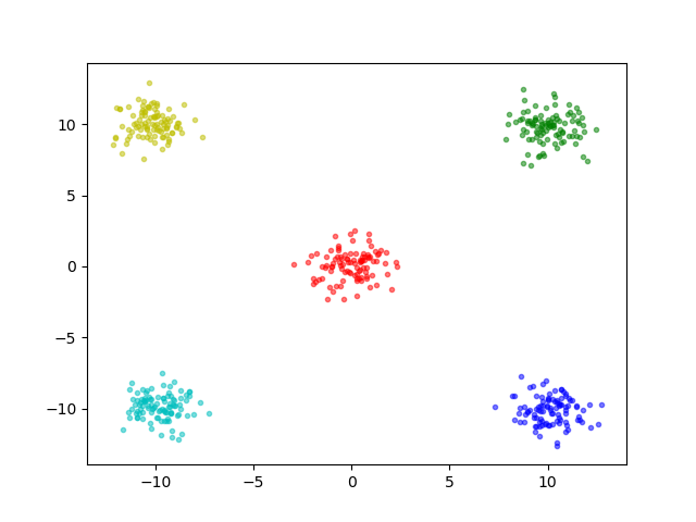
2. sim-2: Five clusters in 2-D (two-dimensional $(R^{2})$ real space). The observations in each of the five clusters are independent bivariate normal random variables with means (0, 0), (10, 10), (10, -10), (-10, 10), and (-10, -10), respectively, and identity covariance matrix. There are 100 observations in each of the 5 clusters, respectively.

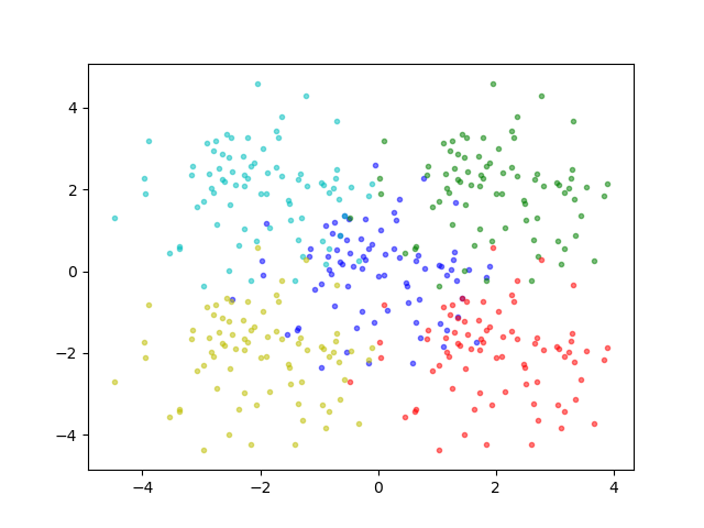
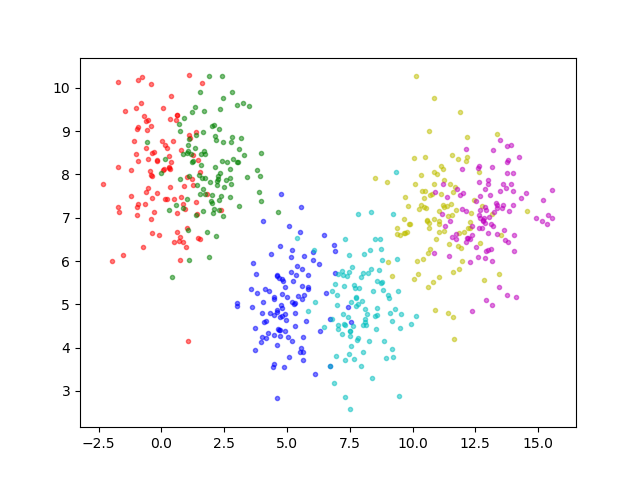
3. sim-3: Five clusters in $R^{2}$. The observations in each of the five clusters are independent bivariate normal random variables with means $(0,0),(2,2),(2,-2),(-2,2),$ and $(-2.-2)$, respectively, and identity covariance matrix. There are 100 observations in each of the 5 clusters.

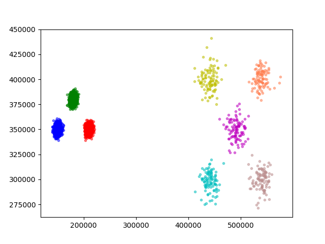
4. sim-4: Eight clusters in $R^{2}$. Five clusters have 100 observations each, and three clusters have 2000 observations each. The observations in each of the clusters are independent bivariate normal random variables with means are similar to [28] and identity covariance matrix.

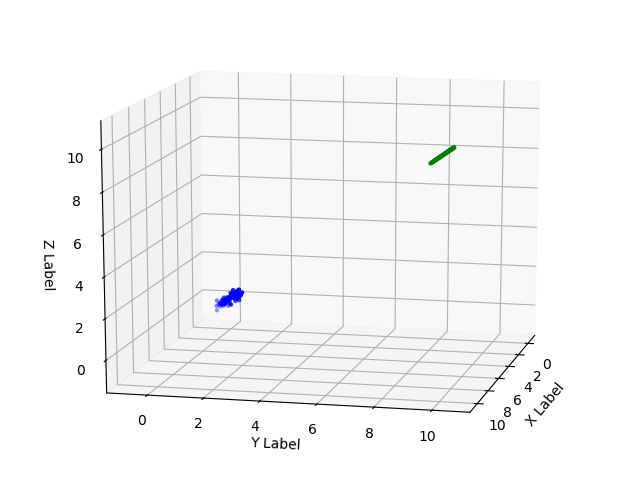
5. sim-5: Two elongated clusters in $R^{3}$. Cluster $1$ contains $100$ observations generated such that each dimension is taking on equally spaced values from $-0.5$ to $0.5$. Gaussian noise with a standard deviation of $0.1$ and $0$ mean is then added to each variable. Cluster $2$ is generated in the same way except that the value $10$ is added to each variable instead of Gaussian noise. This results in two elongated clusters, stretching out along the main diagonal of a three-dimensional cube, with $100$ observations each.

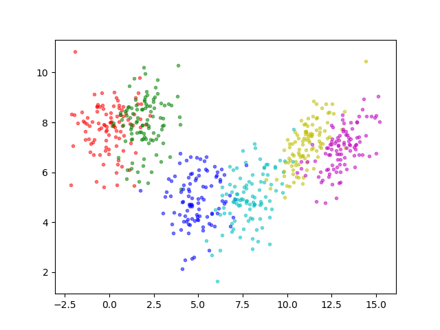
6. sim-6: Six clusters in $R^{2}$. The observations in each of the six clusters are independent bivariate normal random variables with means (0, 8), (2, 8), (5, 5), (8, 5), (11, 7), and (13, 7), respectively, and identity covariance matrix. There are $100$ observations in each of the $6$ clusters, respectively. This simulation is generated to explore cluster overlapping. The distance between centroids of two overlapping clusters is in between 2 and 3.

7. sim-7: Six clusters in $R^{2}$. This simulation is generated as in sim-6. But, we modify the covariance structure. The correlations for six clusters are 0.0, 0.0, 0.3, 0.3, 0.7 and 0.7 corresponding to cluster mean in sim-6.

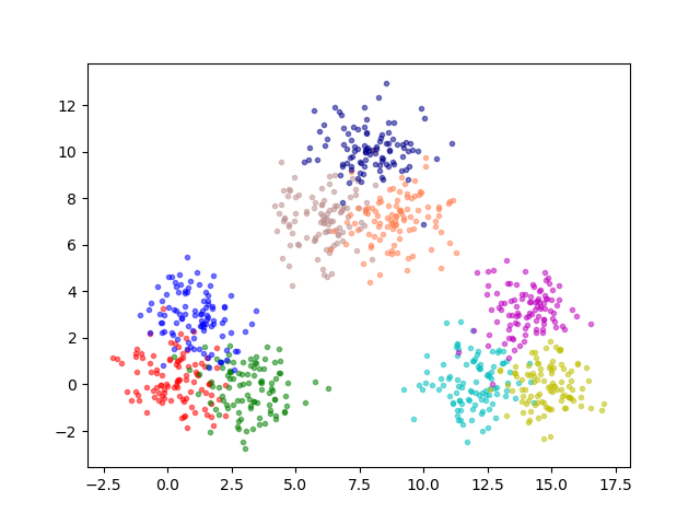
8. sim-8: Nine clusters in $R^{2}$. The observations in each of the nine clusters are independent bivariate normal random variables with means (0, 0), (3, 0), (1, 3), (12, 0), (15, 0), (14, 3), (6,7), (9,7), and (8,10), respectively, and identity covariance matrix. There are $100$ observations in each of the $9$ clusters, respectively. This simulation is simulated with the same purpose of sim-6. But, we made “between-cluster separation” among three groups very small. Also, these groups with three closely space clusters are far from each other.

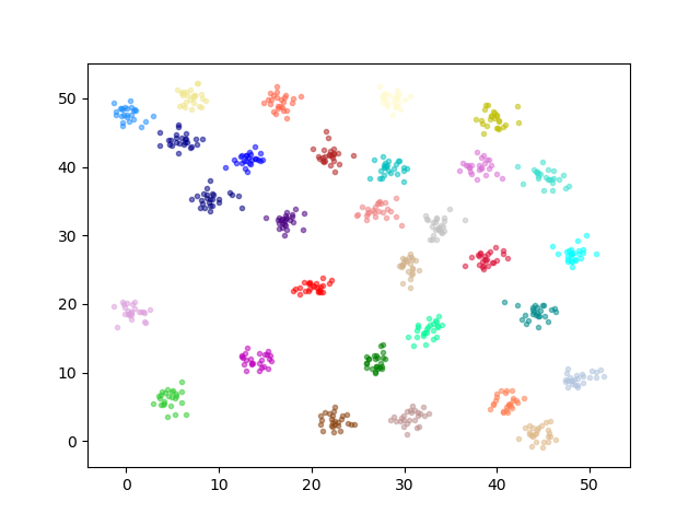
9. sim-9: Thirty clusters in $R^{2}$. Each cluster contains 25 observations. They are an independent bivariate normal random variable with identity covariance matrix and appropriate mean vector. Each mean is randomly generated and has a range between 0 to 50. Any simulation where the Euclidean distance between the mean of two clusters is less than 1, is discarded.

10. sim-10: Four clusters in $R^{4}$. The observations in each of the four clusters are independent multivariate normal random variables with means (1, 10, 30, 50), (10, 30, 50, 70), (30, 50, 70, 90), and (50, 70, 90, 110), respectively, and identity covariance matrices. There are $50500$ observations in each of the four clusters.

11. sim-11: Four clusters in $R^{5}$. The observations in each of the four clusters are independent multivariate normal random variables with means (100, 50, 0, 150, 150), (150, 100, 50, 0, 200), (50, 0, 150, 200, 100), and (0, 200, 100, 50, 150), respectively, and identity covariance matrices. There are $2\times 10^{6}$ observations in each of the 5 clusters.

Table 1: Determination of the size of a sampled dataset with its parameters

Dataset	$\lambda_{max}$	$\tau$	$c$	Sample size(%)	Dataset	$\lambda_{max}$	$\tau$	$c$	Sample size(%)
sim-1	0.079	-	0.2	4	sim-7	22.62	-	0.6	28.72
sim-2	81.20	16	1.32	31	sim-8	36.20	-	0.6	34
sim-3	4.32	-	0.20	50	sim-9	402.88	16	1.45	7
sim-4	19840250263	2	1.00	100	sim-10	1915.54	8	2.57	0.0029
sim-5	75.64	-	0.6	80	sim-11	10435.27	8	3.179	0.000496
sim-6	20.05	-	0.6	60

5.2.2 Prediction of cluster number in SS

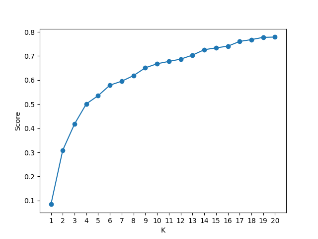
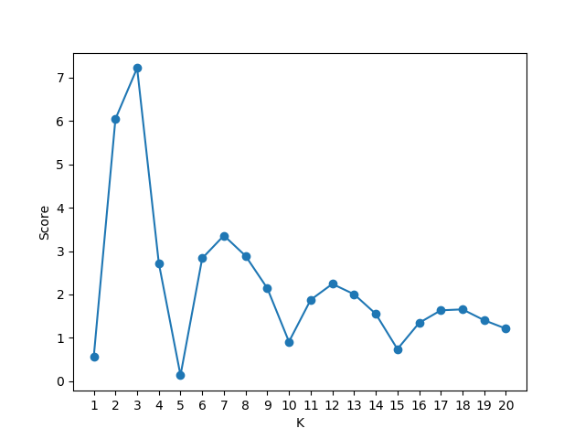
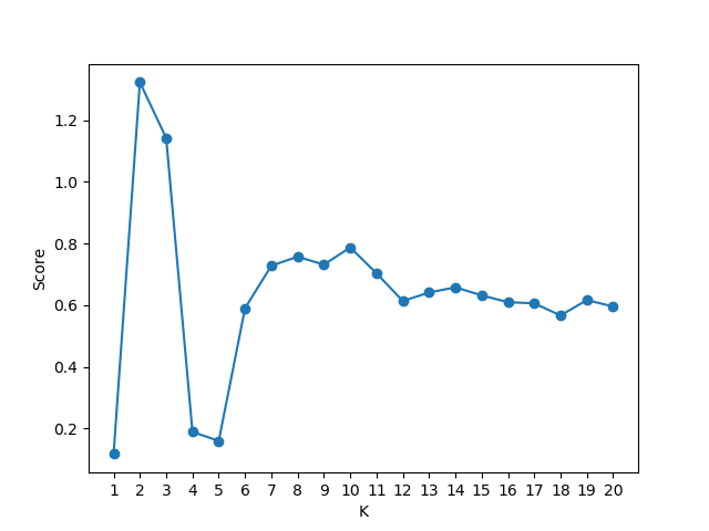
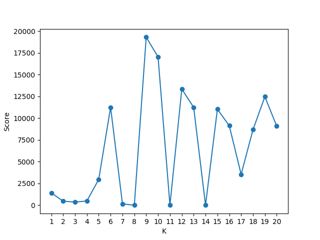
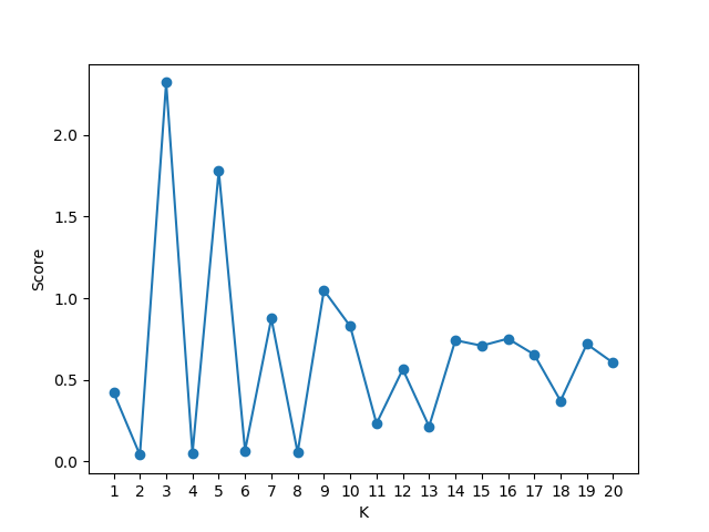
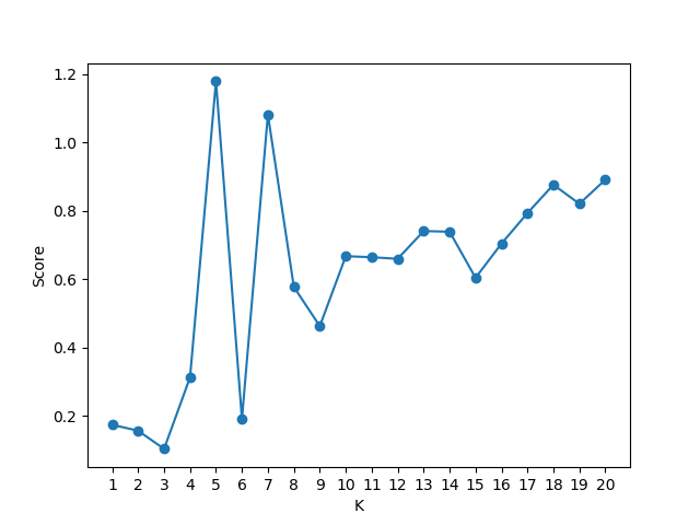
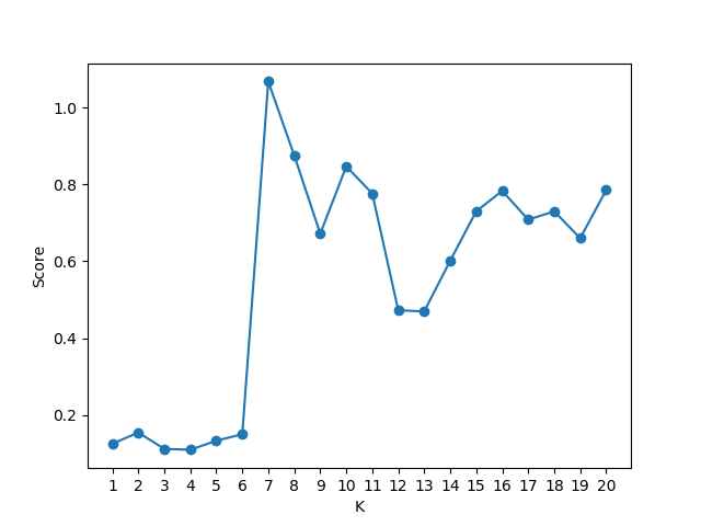
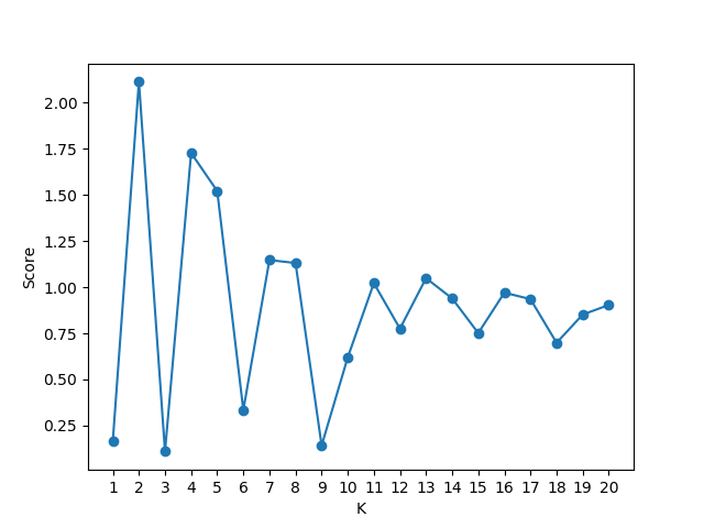
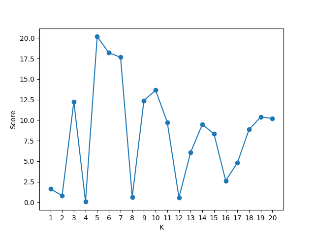
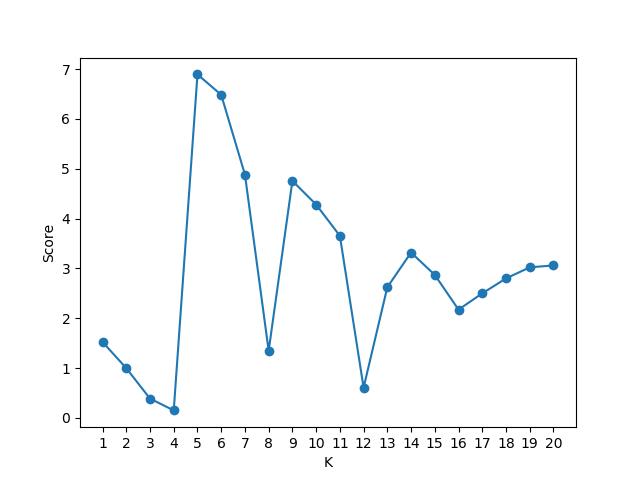
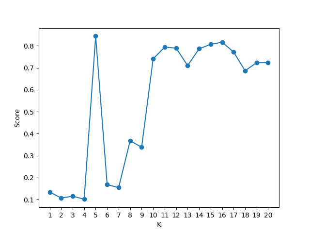
The proposed method CNAK compared with seven existing methods presented in Section 4.1. We have generated 50 realizations for each of the simulation in SS. We have shown the outcome of the methods in Table 2. We put “*” in the cell where the prediction is disseminated over many values between $k_{min}$ to $k_{max}$ for 50 realizations. Hence, conclusion can not be drawn. We put “-” where execution time for a single realization is very high, and use “$\times$” where methods are not applicable. We follow this throughout our paper. Results on sim-1 suggest that CNAK can predict a single cluster. Therefore, it can indicate whether clustering is required at all. Though the gap is another popular method in the literature which can predict such a situation, it fails to perform in our simulation (sim-1). However, CNAK indicates a single cluster for sim-3. We made “between-cluster separation” very small for sim-3 (shown in Figure 1(b)). Therefore, it appears as a single cluster. This situation can be circumvented by looking at the plot of “k vs. score” with detailed analysis. Figure 2(c) shows another dip at $k=5$, which is the second minimum score, computed by the CNAK. The experimental simulation shows that CNAK is good at identifying well-separated clusters (sim-3 and sim-5) as the other methods under comparison. We also study the robustness of prediction techniques in the presence of cluster imbalance. ‘Cluster imbalance’ is a phenomenon where the number of instances for representing a few groups is small compared to the other groups. Results indicate that the CNAK along with the curvature, silhouette, and jump methods can take care of cluster imbalance. Another advantage of our approach is to estimate cluster number for a large dataset which contains more than a million instances. CNAK takes only 34.57 seconds and 45 minutes for executing sim-10 and sim-11, respectively. On the other hand, other comparing methods take hours to days. To justify the performance of CNAK, we generate a score ($gs$) using Eq. 16.

$$\begin{array}[]{lll}gs&=&\exp^{-(\dfrac{k_{True}-k_{X}}{\sigma})^{2}}\end{array}$$ (16)

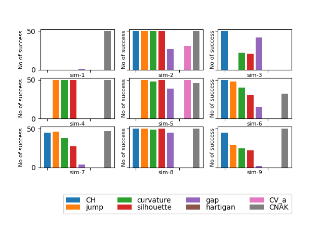
Where $k_{True}$ is the ground truth of the dataset, and $k_{X}$ is the predicted cluster number by method $X$. We set $\sigma=2$ for our experiment. The value of gs lies between 0 to 1. Higher its value, better is the estimation. We consider gs-score to be 0 for sim-1, sim-10, and sim-11 if any method is not able to compute their score for $k=1$, or is not possible to execute within a reasonable execution time. To summarize, we have shown a bar graph for true $k$ in Figure 3, which indicates the consistent and comparable behavior of CNAK.Average gs score in Table 2 indicates consistent behavior of the CNAK for all simulations under consideration. We have highlighted the best performances in bold font. The novel contributions in our approach are correct identification of the single cluster $k=1$, and fast computation for estimating the number of clusters in big data.

(a) sim-1

(b) sim-2

(c) sim-3

(d) sim-4

(e) sim-5

(f) sim-6

(g) sim-7

(h) sim-8

(i) sim-9

(j) sim-10

(k) sim-11

Figure 2: plot of “k vs Score”. Score is generated by CNAK

Table 2: Prediction of cluster number based on the mode of accumulated estimation of 50 realizations.

Dataset	True K	Comparison of seven approached in cluster number prediction
		CH	Jump	Hartigan	Curvature	Silhouette	Gap	$CV_{a}$	CNAK
sim-1	1	$\times$	$\times$	$\times$	$\times$	$\times$	$*$	$\times$	1
sim-2	5	5	5	*	5	5	5	5	5
sim-3	5	5	4	*	5	4	5	4	1
sim-4	8	14	8	*	8	8	17	7	8
sim-5	2	20	2	9	2	2	2	2	2
sim-6	3,6	3	3	*	3	3	3	2	3
sim-7	3,6	3	3	*	*	3	4	2	3
sim-8	3,9	3	3	*	3	3	3	3	3
sim-9	30	30	30	32	30	29,30	35	2	30
sim-10	4	-	-	-	-	-	-	-	4
sim-11	4	-	-	-	-	-	-	-	4
Average gs-score		0.524	0.706	0.000	0.564	0.687	0.596	0.626	0.904

Figure 3: Prediction of cluster number by eight methods. For each of the ten simulations (in SS), the bar plots represent the number of successful attempts (out of 50 realizations) where true cluster number is predicted.

5.2.3 Clustering on Synthetic Dataset (SS)

Table 3: Clustering results on the synthetic simulations (sim2-sim7)

Dataset Methods K ARI NMI Homogeneity Completeness Silhouette Mode SM Mode SM Mode SM Mode SM Mode SM sim-2 CNAK 5 1.00 1.00 1.00 1.00 1.00 1.00 1.00 1.00 0.91 0.91 BA 5 1.00 1.00 1.00 1.00 1.00 1.00 1.00 1.00 0.91 0.91 RS 5 1.00 1.00 1.00 1.00 1.00 1.00 1.00 1.00 0.91 0.91 RPKM 5 0.78 0.83 0.91 0.93 0.83 0.87 0.99 0.99 0.51 0.36 sim-3 CNAK 5 0.68 0.64 0.69 0.66 0.69 0.57 0.69 0.66 0.60 0.59 BA 5 0.63 0.63 0.64 0.63 0.63 0.63 0.64 0.64 0.56 0.56 RS 5 0.66 0.66 0.67 0.68 0.67 0.68 0.68 0.67 0.54 0.54 RPKM 5 0.55 0.63 0.60 0.63 0.58 0.63 0.61 0.64 0.51 0.41 sim-4 CNAK 8 1.00 1.00 1.00 1.00 1.00 1.00 1.00 1.00 0.99 0.99 BA 8 1.00 1.00 1.00 1.00 1.00 1.00 1.00 1.00 0.99 0.99 RS 8 1.00 1.00 1.00 1.00 1.00 1.00 1.00 1.00 0.99 0.99 RPKM 8 1.00 1.00 1.00 1.00 1.00 1.00 1.00 1.00 0.99 0.99 sim-5 CNAK 2 1.00 1.00 1.00 1.00 1.00 1.00 1.00 1.00 0.96 0.96 BA 2 1.00 1.00 1.00 1.00 1.00 1.00 1.00 1.00 0.96 0.96 RS 2 1.00 1.00 1.00 1.00 1.00 1.00 1.00 1.00 0.96 0.96 RPKM 2 1.00 1.00 1.00 1.00 1.00 1.00 1.00 1.00 0.96 0.96 sim-6 CNAK 3 0.88 0.88 0.83 0.83 0.83 0.83 0.83 0.83 0.79 0.78 6 0.47 0.47 0.64 0.64 0.81 0.82 0.50 0.50 0.58 0.59 BA 3 0.87 0.87 0.82 0.83 0.82 0.83 0.82 0.83 0.79 0.79 6 0.53 0.52 0.66 0.64 0.64 0.62 0.64 0.64 0.23 0.243 RS 3 0.88 0.88 0.83 0.83 0.83 0.83 0.83 0.83 0.80 0.80 6 0.63 0.64 0.72 0.72 0.67 0.68 0.67 0.68 0.53 0.52 RPKM 3 0.64 0.64 0.64 0.64 0.63 0.63 0.64 0.64 0.39 0.39 6 0.66 0.61 0.71 0.69 0.71 0.67 0.71 0.71 0.40 0.37 sim-7 CNAK 3 0.93 0.93 0.90 0.90 0.90 0.90 0.90 0.90 0.57 0.57 6 0.65 0.65 0.73 0.73 0.73 0.73 0.73 0.73 0.40 0.40 BA 3 0.85 0.83 0.82 0.80 0.82 0.79 0.82 0.80 0.55 0.53 6 0.61 0.61 0.71 0.69 0.71 0.70 0.70 0.69 0.30 0.30 RS 3 0.52 0.52 0.70 0.70 0.55 0.55 0.89 0.89 0.58 0.58 6 0.62 0.61 0.71 0.69 0.71 0.69 0.71 0.69 0.31 0.30 RPKM 3 0.61 0.52 0.55 0.58 0.58 0.53 0.66 0.65 0.53 0.48 6 0.44 0.48 0.60 0.59 0.53 0.51 0.68 0.69 0.34 0.30

Table 4: Clustering results on the synthetic simulations (sim8-sim12)

Dataset Methods K ARI NMI Homogeneity Completeness Silhouette Mode SM Mode SM Mode SM Mode SM Mode SM sim-8 CNAK 3 1.00 1.00 1.00 1.00 1.00 1.00 1.00 1.00 0.99 0.99 9 0.61 0.58 0.72 0.71 0.72 0.70 0.72 0.71 0.39 0.38 BA 3 1.00 1.00 1.00 1.00 1.00 1.00 1.00 1.00 0.94 0.94 9 0.54 0.51 0.68 0.67 0.68 0.67 0.69 0.67 0.25 0.22 RS 3 1.00 1.00 1.00 1.00 1.00 1.00 1.00 1.00 0.94 0.94 9 0.57 0.57 0.71 0.71 0.70 0.71 0.72 0.71 0.28 0.29 RPKM 3 1.00 0.98 1.00 0.99 1.00 0.98 1.00 0.99 0.76 0.75 9 0.53 0.51 0.69 0.69 0.64 0.64 0.74 0.74 0.30 0.35 sim-9 CNAK 30 0.99 0.99 0.99 0.99 0.99 0.99 0.99 0.99 0.75 0.75 BA 30 0.38 0.39 0.71 0.71 0.70 0.70 0.71 0.71 -0.17 -0.17 RS 30 0.77 0.77 0.94 0.94 0.90 0.90 0.94 0.94 0.64 0.63 RPKM 30 0.69 0.69 0.88 0.89 0.87 0.87 0.92 0.91 0.49 0.48 sim-10 CNAK 4 0.97 0.97 0.96 0.96 0.96 0.96 0.96 0.96 - - BA 4 0.96 0.93 0.94 0.92 0.94 0.92 0.94 0.92 - - RS 4 0.97 0.96 0.96 0.95 0.96 0.95 0.96 0.95 - - RPKM 4 0.47 0.46 0.62 0.62 0.56 0.53 0.70 0.73 - - sim-11 CNAK 4 1.00 1.00 1.00 1.00 1.00 1.00 1.00 1.00 - - BA 4 1.00 0.94 1.00 0.97 1.00 0.95 1.00 0.99 - - RS 4 0.71 0.72 0.87 0.86 0.75 0.76 0.99 0.99 - - RPKM 4 0.71 0.65 0.87 0.80 0.80 0.69 0.99 0.94 - -

By evaluating the quality of clustering, we may judge and validate the predicted cluster number. Table 3 and  4 suggest whether our proposed method produces a good clustering with its predicted cluster number. We have designed a pair of simulations to examine the performance of methods in the context of “between-cluster separation”, “tolerance against noise variables”, “correlation between feature variables”, “cluster hierarchy” and “large scale dataset”. Sim-2 and sim-3 reveal that the performance of CNAK deteriorates with decreasing “between-cluster separation”. The CNAK can detect the presence of hierarchical clustering structure. But, its performance in clustering declines at an individual level. It is to be noted that a few closely spaced clusters form a big cluster. This is how we define the hierarchy in the simulation. This might be the reason of performance drop at an individual level, as suggested by the scores of k=3 and 6 for sim-6 in Table 3. Also, we observe that clustering improves in sim-7. Here, we add a positive correlation between two variables in the covariance matrix while generating this simulation. Finally, we have seen that CNAK and bootstrap-averaging techniques produce similar value for clustering outcome except for sim-9. This shows that our proposed method is robust against a large cluster number. Due to a large number of instances (sim-10 and sim-11), we are not able to compute the silhouette score. However, the advantage of our proposed method is a large reduction in execution time without compromising accuracy. Also, we designed two single simulations to measure the performance in the case of “unbalanced clustering” and the presence of “many clusters”. Like other comparable methods, CNAK can handle unbalanced clustering situation as suggested by the performance measures for sim-4. However, with many clusters, our method performs the best among all other comparable methods. We have highlighted the best performing clustering algorithm and the values of its performance measures in Tables 3, and  4. In summary, the CNAK is able to detect whether a dataset forms a single cluster. It is also capable of determining a large number of clusters, efficient in large scale dataset. But, its performance declines with decreasing “between-cluster separation” as expected like any other k-means clustering based method.

5.2.4 Study on overlapping clusters (sim-g1)

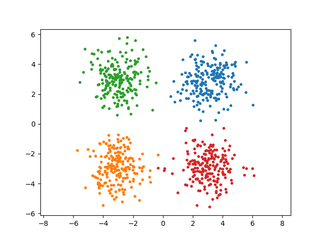
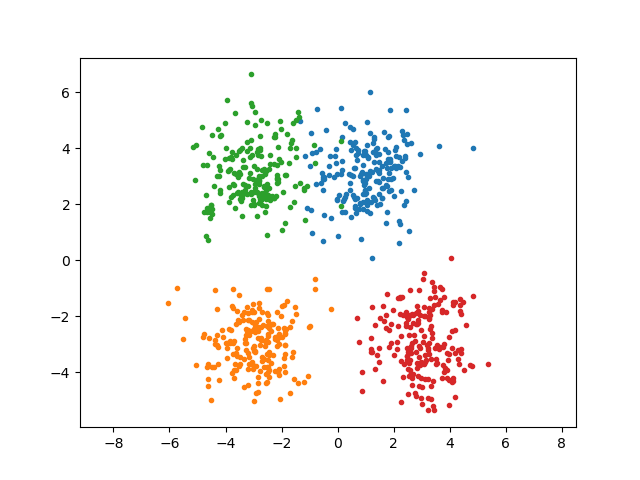
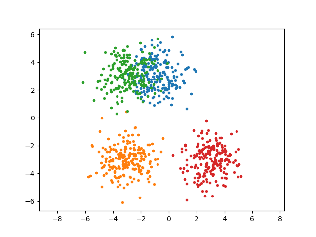
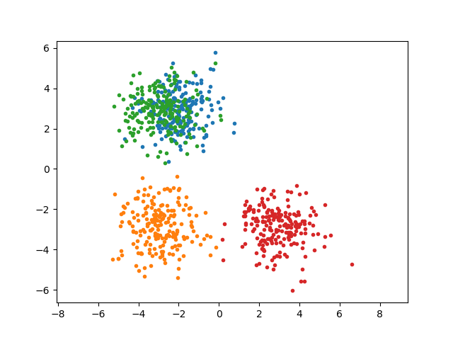
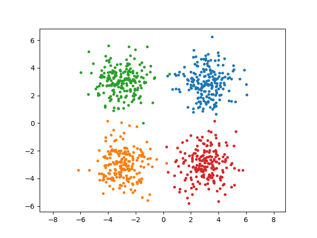
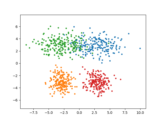
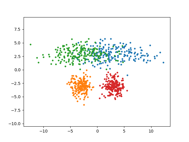
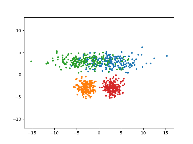
We consider Gaussian clusters and tune their parameters (centers, cluster shape, and spread, covariance matrices, etc.) to generate overlapping between two clusters. In this work, we tune “distance between cluster centroids” and covariance matrices to create simulations. For this purpose, we generate four Gaussian clusters which are spaced in a square with the length of its side 6. Each cluster has an identity covariance matrix. We introduce the intermix between clusters by moving one cluster centroid closer to another. Figure 4 presents the datasets with distances between two cluster centroids kept at 6, 4, 2 and 1. Additionally, we create another set of overlapping simulation based on changing covariance matrices. We multiply identity covariance matrices of two clusters by 5, 10 and 15, respectively. We have shown them in Figure 5. It is difficult to identify two clusters (shown in blue and green colors) separately in Figures 4(c) and 4(d) visually. Results (Table 5) corroborates with visual findings. It is noted that predictions of all the methods (except “Hartigan” and $CV_{a}$) synchronized with visual findings when overlapping is generated by changing the position of cluster centroids. However, every method has mixed responses in the second scenario. Jump, and CNAK correctly predict the cluster number as 4 in all the four cases. The CNAK shows diverse responses in 50 trials against cov-10I and cov-15I.

(a) dist-6

(b) dist-4

(c) dist-2

(d) dist-1

Figure 4: Cluster intermix based on distance between cluster centroids

(a) cov-I

(b) cov-5I

(c) cov-10I

(d) cov-15I

Figure 5: Cluster intermix based on $n*I$ covariance matrices of two clusters where n is an integer. Other two clusters have $I$ covariance matrices. $I$ represents Identity matrix.

Table 5: Effects on performances for prediction of cluster number for cluster overlapping

Dataset	Comparison of seven approached in cluster number prediction
	CH	Jump	Hartigan	Curvature	Silhouette	Gap	$CV_{a}$	CNAK
dist-6	4	4	42	4	4	4	4	4
dist-4	4	4	44	4	4	4	2	4, 3
dist-2	3	3	36	3	3	4	2	3
dist-1	3	3	35	3	3	3	2	3
cov-I	4	4	38	4	4	4	4	4
cov-5I	5	4	48	17	4	4	4	4
cov-10I	7	4	34	19	5	5	2	4, 5, 2
cov-15I	6	4	32	4	5	6	2	4, 2
average gs	0.726	0.947	0.000	0.695	0.838	0.865	0.605	0.945

Tables 6 and 7 present the performance of clustering with the predicted cluster number. In general, the accuracy of clustering with respect to the ground truth decreases with increasing overlapping. It is interesting to note that with increasing clustering accuracy from $k=3$ to $4$, the silhouette score decreases. This is an indicator of reduced “between-cluster separation”.

Table 6: Clustering results on simulation designed for cluster Intermix (non-hierarchical) by changing distance between cluster centroid

Dataset Methods K ARI NMI Homogeneity Completeness Silhoutte Mode SM Mode SM Mode SM Mode SM Mode SM dist-6 CNAK 4 1.00 1.00 1.00 1.00 1.00 1.00 1.00 1.00 0.70 0.70 BA 4 0.99 0.99 0.99 0.99 0.99 0.99 0.99 0.99 0.81 0.81 RS 4 0.99 0.99 0.99 0.99 0.99 0.99 0.99 0.99 0.81 0.81 RPKM 4 0.99 0.99 0.98 0.98 0.98 0.98 0.98 0.98 0.67 0.66 dist-4 CNAK 4 0.98 0.98 0.97 0.97 0.97 0.97 0.97 0.97 0.64 0.64 BA 4 0.96 0.93 0.94 0.92 0.94 0.92 0.94 0.92 0.76 0.74 RS 4 0.97 0.96 0.96 0.95 0.96 0.95 0.95 0.95 0.77 0.76 RPKM 4 0.90 0.93 0.92 0.91 0.92 0.90 0.92 0.93 0.59 0.59 dist-2 CNAK 3 0.70 0.70 0.85 0.85 0.73 0.73 0.98 0.98 0.64 0.64 4 0.94 0.94 0.93 0.93 0.93 0.93 0.93 0.93 0.59 0.59 BA 3 0.70 0.69 0.85 0.83 0.73 0.72 0.98 0.96 0.51 0.49 4 0.69 0.72 0.79 0.78 0.77 0.76 0.83 0.81 0.43 0.48 RS 3 0.71 0.71 0.85 0.85 0.74 0.74 0.98 0.98 0.51 0.51 4 0.62 0.62 0.78 0.78 0.73 0.73 0.83 0.83 0.36 0.36 RPKM 3 0.70 0.70 0.85 0.85 0.73 0.73 0.98 0.98 0.66 0.66 4 0.74 0.71 0.81 0.80 0.80 0.78 0.83 0.84 0.52 0.52 dist-1 CNAK 3 0.71 0.71 0.86 0.86 0.74 0.74 0.99 0.99 0.66 0.66 4 0.99 0.99 0.99 0.99 0.99 0.99 0.99 0.99 0.54 0.54 BA 3 0.71 0.71 0.86 0.85 0.74 0.74 0.98 0.98 0.51 0.51 4 0.69 0.68 0.77 0.78 0.73 0.73 0.89 0.83 0.43 0.42 RS 3 0.71 0.71 0.86 0.86 0.74 0.74 0.99 0.99 0.51 0.50 4 0.62 0.62 0.78 0.78 0.73 0.73 0.84 0.84 0.37 0.37 RPKM 3 0.71 0.71 0.85 0.85 0.74 0.74 0.99 0.99 0.68 0.68 4 0.64 0.66 0.80 0.81 0.74 0.74 0.86 0.88 0.59 0.59

Table 7: Clustering results on simulation designed for cluster Intermix (non-hierarchical) by changing covariance matrix

Dataset Methods ARI NMI Homogeneity Completeness Silhoutte Mode SM Mode SM Mode SM Mode SM Mode SM cov_I CNAK 4 0.99 0.99 0.99 0.99 0.99 0.99 0.99 0.99 0.69 0.69 BA 4 0.98 0.98 0.97 0.97 0.97 0.97 0.97 0.97 0.80 0.79 RS 4 0.98 0.98 0.97 0.97 0.97 0.97 0.97 0.97 0.80 0.80 RPKM 4 0.99 0.95 0.98 0.95 0.98 0.94 0.98 0.96 0.66 0.64 cov_5I CNAK 4 0.91 0.91 0.90 0.90 0.906 0.905 0.90 0.90 0.59 0.59 BA 4 0.98 0.98 0.97 0.97 0.97 0.97 0.97 0.97 0.80 0.80 RS 4 0.87 0.88 0.88 0.88 0.88 0.88 0.88 0.88 0.69 0.69 RPKM 4 0.85 0.74 0.86 0.79 0.85 0.77 0.86 0.82 0.57 0.50 cov_10I CNAK 4 0.81 0.81 0.84 0.83 0.83 0.83 0.84 0.84 0.55 0.55 BA 4 0.78 0.68 0.78 0.72 0.79 0.72 0.77 0.73 0.58 0.47 RS 4 0.78 0.78 0.81 0.81 0.81 0.81 0.81 0.81 0.59 0.59 RPKM 4 0.46 0.49 0.63 0.64 0.52 0.55 0.76 0.74 0.34 0.37 cov_15I CNAK 4 0.79 0.79 0.82 0.82 0.82 0.82 0.82 0.82 0.56 0.56 BA 4 0.73 0.64 0.77 0.69 0.77 0.69 0.77 0.70 0.54 0.43 RS 4 0.77 0.77 0.81 0.81 0.81 0.81 0.81 0.81 0.59 0.58 RPKM 4 0.47 0.50 0.63 0.62 0.51 0.55 0.77 0.71 0.35 0.39

5.2.5 Study on high dimensional dataset (sim-g2)

Table 8: A brief description of synthetic high dimensional dataset. ($\lambda_{max}$, $\tau$, $c$) are the parameters for the determination of the size of sampled dataset as discussed in section 3.

Dataset	Instances	Features	Classes	$\lambda_{max}$	$\tau$	c	Sample size (%)
dim32	1024	32	16	17866.16	4	11.56	34
dim64	1024	64	16	22870.62	4	12.30	36
dim128	1024	128	16	34119.84	4	13.59	41
dim256	1024	256	16	67076.31	3	16.09	13
dim512	1024	512	16	122947.96	3	49.72	16
dim1024	1024	1024	16	235344.67	3	61.74	19

We consider six high dimensional datasets [15] dim32 to dim1024 with higher dimensionality varying from 32 to 1,024. Clusters are distinctly separated. We summarize its features in Table 8. We examine the robustness of different methods against the large dimensional dataset. We find in Table 9 that CH, Silhouette, and CNAK are capable of predicting true cluster numbers whereas others fail. However, the results of clustering in Table 10 shows that CNAK performs comparatively better than other methods. Additionally, we add white Gaussian noise such that SNR value ranges from 100dB to 30dB. There is no such change in the results while perturbing this simulation with noise.

Table 9: Effects on Performances for prediction of cluster number with increasing feature dimension. Overflow encountered in double_scalars for jump dataset for dimension of feature greater than 64.

Dataset	K	Comparison of seven approaches in Cluster Number Prediction
		CH	Jump	Hartigan	Curvature	Silhouette	Gap	$CV_{a}$	CNAK
dim32	16	16	14	16	14	16	23	11	16
dim64	16	16	14	17	14	16	24	13	16
dim128	16	16	-	18	14	16	22	21	16
dim256	16	16	-	16	14	16	25	21	16
dim512	16	16	-	16	14	16	24	21	16
dim1024	16	16	-	16	14	16	23	23	16
Average gs score		1.00	-	0.857	0.37	1.00	0.00	0.01	1.00

Table 10: Clustering results on the simulation designed for checking scalability (increasing number of dimensions). Results are shown for two k appear in sorted score (ascending order)

Dataset Methods ARI NMI Homogeneity Completeness Silhoutte Mode SM Mode SM Mode SM Mode SM Mode SM dim32 CNAK 1.00 1.00 1.00 1.00 1.00 1.00 1.00 1.00 0.99 0.99 BA 0.94 0.91 0.98 0.98 0.97 0.96 1.00 0.99 0.87 0.84 RS 0.74 0.71 0.93 0.92 0.87 0.85 1.00 1.00 0.66 0.68 RPKM 0.17 0.18 0.58 0.58 0.35 0.35 1.00 0.98 0.21 0.20 dim64 CNAK 1.00 1.00 1.00 1.00 1.00 1.00 1.00 1.00 0.99 0.99 BA 0.88 0.90 0.97 0.97 0.97 0.95 1.00 0.99 0.89 0.85 RS 0.32 0.32 0.76 0.75 0.58 0.57 1.00 1.00 0.41 0.38 RPKM 0.11 0.13 0.55 0.53 0.30 0.29 1.00 0.97 0.19 0.17 dim128 CNAK 1.00 1.00 1.00 1.00 1.00 1.00 1.00 1.00 0.99 0.99 BA 0.94 0.92 0.98 0.98 0.97 0.96 1.00 0.99 0.91 0.88 RS 0.53 0.60 0.86 0.86 0.74 0.74 1.00 0.99 0.58 0.55 RPKM 0.11 0.13 0.54 0.53 0.30 0.29 1.00 0.98 0.18 0.16 dim256 CNAK 1.00 1.00 1.00 1.00 1.00 1.00 1.00 1.00 0.99 0.99 BA 0.88 0.92 0.97 0.98 0.94 0.96 1.00 0.99 0.92 0.89 RS 0.60 0.57 0.89 0.87 0.79 0.76 1.00 1.00 0.59 0.57 RPKM 0.11 0.14 0.56 0.55 0.31 0.31 1.00 0.99 0.18 0.17 dim512 CNAK 1.00 1.00 1.00 1.00 1.00 1.00 1.00 1.00 0.99 0.99 BA 0.88 0.90 0.97 0.97 0.94 0.95 1.00 0.99 0.92 0.88 RS 0.37 0.35 0.77 0.76 0.54 0.59 1.00 0.99 0.47 0.38 RPKM 0.11 0.14 0.58 0.53 0.29 0.30 1.00 0.99 0.18 0.17 dim1024 CNAK 1.00 1.00 1.00 1.00 1.00 1.00 1.00 1.00 0.99 0.99 BA 0.94 0.90 0.98 0.97 0.97 0.95 1.00 0.99 0.93 0.90 RS 0.63 0.58 0.88 0.87 0.79 0.76 1.00 1.00 0.61 0.58 RPKM 0.17 0.16 0.60 0.57 0.36 0.33 1.00 0.99 0.18 0.19

5.2.6 Study on Shape clusters (sim-g3)

(a) Aggregation

(b) Compound

(c) Pathbased

(d) Spiral

(e) Flame

(f) Jain

(g) R15

(h) D31

Figure 6: Datasets of different shape structure

Table 11: A brief description of synthetic shape dataset. ($\lambda_{max}$, $\tau$, $c$) are the parameters for the determination of the size of sampled dataset as discussed in section 3.

Dataset	Instances	Features	Classes	$\lambda_{max}$	$\tau$	c	Sample size (%)
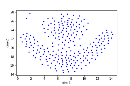
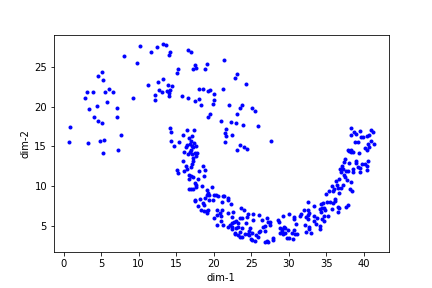
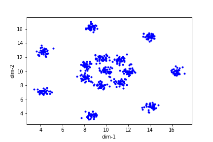
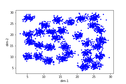
Aggregation [17]	788	2	7	98.49	16	1.33	21
Compound [37]	399	2	6	97.68	16	1.33	35
Path-based [5]	300	2	3	68.12	16	1.30	34
Spiral [5]	312	2	3	53.29	16	1.28	29
Flame [16]	240	2	2	11.47	-	0.2	82
Jain [24]	373	2	2	103	16	1.34	39
R15 [34]	600	2	15	10.67	-	0.2	63
D31 [34]	3100	2	31	55.75	-	0.2	63

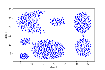
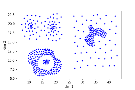
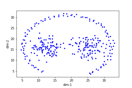
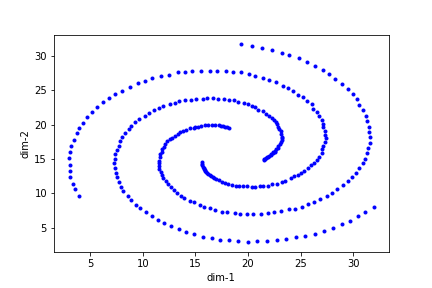
This simulation is used to compare the methods on different shape datasets [17, 37, 5, 34, 16, 24]. We provide their brief description in Table 11. Table 12 affirms the limitation of CNAK towards different shape identification, which is an inherent limitation of the k-means algorithm. R15 and D31 may contain many small spherical clusters as shown in Figure 6(g) and 6(h), respectively. This might be the reason behind successful prediction for these two datasets by CNAK, CH, and silhouette. Clustering outcome in Table 13 confirms the findings with $ARI$ and $NMI$ $>0.9$ in D31 and R15.

Table 12: Performances of cluster number prediction in different shape datasets

Dataset	K	Comparison of seven approaches in Cluster Number Prediction
		CH	Jump	Hartigan	Curvature	Silhouette	Gap	$CV_{a}$	CNAK
Aggregation [17]	7	26	2	37	30	4	16	2	6
Compound [37]	6	2	3	26	10	2	11	2	3
pathbased [5]	3	26	9	28	28	3	2	2	2
spiral [5]	3	26	26	18	19	25	1	20	8
Flame [16]	2	8	2	15	24	4	8	11	7
Jain [24]	2	20	4	21	25	7	13	2	2
R15 [34]	15	15	13	20	13	15	18	7	15
D31 [34]	31	31	25	57	29	31	36	2	31
Average gs score		0.25	0.23	0.00	0.09	0.43	0.16	0.14	0.58

Table 13: Clustering results on shape dataset with cluster number predicted by CNAK and ground truth

Dataset Methods K ARI NMI Homogeneity Completeness Silhoutte Mode SM Mode SM Mode SM Mode SM Mode SM Aggregation CNAK 6 0.80 0.80 0.87 0.87 0.88 0.88 0.87 0.87 0.48 0.48 7 0.72 0.72 0.83 0.83 0.88 0.88 0.79 0.79 0.47 0.47 BA 6 0.62 0.61 0.74 0.75 0.74 0.75 0.74 0.75 0.34 0.37 7 0.67 0.65 0.81 0.80 0.86 0.85 0.77 0.76 0.42 0.41 RS 6 0.79 0.79 0.88 0.88 0.88 0.88 0.87 0.87 0.48 0.48 7 0.73 0.73 0.84 0.84 0.88 0.88 0.79 0.79 0.47 0.47 RPKM 6 0.43 0.41 0.61 0.61 0.49 0.47 0.77 0.77 0.44 0.43 7 0.43 0.40 0.61 0.60 0.49 0.47 0.77 0.77 0.44 0.43 Compound CNAK 3 0.73 0.73 0.79 0.79 0.65 0.65 0.96 0.96 0.61 0.61 6 0.55 0.55 0.70 0.69 0.72 0.73 0.67 0.66 0.41 0.41 BA 3 0.73 0.73 0.79 0.79 0.65 0.65 0.96 0.96 0.61 0.61 6 0.56 0.56 0.70 0.70 0.71 0.71 0.68 0.69 0.38 0.38 RS 3 0.73 0.73 0.79 0.79 0.65 0.65 0.96 0.96 0.61 0.61 6 0.59 0.55 0.74 0.71 0.77 0.74 0.71 0.68 0.43 0.42 RPKM 3 0.74 0.65 0.82 0.76 0.67 0.60 1.00 0.97 0.57 0.57 6 0.74 0.58 0.82 0.72 0.67 0.54 1.00 0.96 0.57 0.58 Pathbased CNAK 2 0.40 0.40 0.50 0.50 0.40 0.40 0.63 0.63 0.51 0.51 3 0.46 0.46 0.55 0.55 0.52 0.52 0.58 0.58 0.54 0.54 BA 2 0.40 0.40 0.50 0.50 0.40 0.40 0.63 0.63 0.51 0.51 3 0.46 0.46 0.54 0.54 0.52 0.51 0.58 0.57 0.53 0.53 RS 2 0.40 0.40 0.50 0.50 0.40 0.40 0.63 0.63 0.51 0.51 3 0.46 0.46 0.55 0.55 0.52 0.52 0.58 0.58 0.54 0.54 RPKM 2 0.39 0.37 0.50 0.46 0.43 0.41 0.63 0.52 0.51 0.45 3 0.37 0.36 0.44 0.44 0.43 0.41 0.46 0.47 0.43 0.42 Jain CNAK 2 0.55 0.55 0.51 0.51 0.55 0.55 0.47 0.47 0.50 0.50 BA 2 0.54 0.54 0.50 0.50 0.54 0.54 0.47 0.47 0.50 0.50 RS 2 0.55 0.55 0.51 0.51 0.55 0.55 0.47 0.47 0.50 0.50 RPKM 2 0.32 0.32 0.34 0.34 0.44 0.44 0.26 0.26 0.32 0.32 R15 CNAK 15 0.99 0.99 0.99 0.99 0.99 0.99 0.99 0.99 0.75 0.75 BA 15 0.86 0.83 0.92 0.91 0.98 0.96 0.87 0.86 0.48 0.44 RS 15 0.91 0.88 0.96 0.95 0.95 0.93 0.98 0.97 0.71 0.69 RPKM 15 0.18 0.17 0.53 0.53 0.33 0.33 0.85 0.86 0.27 0.26 D31 CNAK 31 0.95 0.95 0.96 0.96 0.97 0.97 0.97 0.97 0.58 0.58 BA 31 0.52 0.51 0.82 0.81 0.77 0.76 0.86 0.86 0.28 0.27 RS 31 0.72 0.69 0.90 0.88 0.87 0.85 0.92 0.92 0.49 0.48 RPKM 31 0.09 0.09 0.50 0.50 0.27 0.27 0.90 0.90 0.39 0.38

5.3 Real-World Datasets

To check the performance of the CNAK algorithm in real-world datasets, we have selected iris, wine, seed, breast-cancer, landsat-satellite, and magic from the UCI repository [9]. We provide a brief description of these datasets in Table 14.

Table 14: A brief description of real-world datasets. ($\lambda_{max}$, $\tau$, $c$) are the parameters for the determination of the size of sampled dataset.

Dataset	Instances	Feature Dimension	$\lambda_{max}$	$\tau$	$c$	Sample Size (%)
iris	150	4	4.22	-	0.6	24
wine	400	13	99201.79	3	46.29	49
seed	480	7	10.79	-	0.6	35
breast-cancer	720	9	49.047	16	1.275	14
landsat satellite	6435	36	5757.44	16	1.72	54
magic	19020	10	6579.79	8	3	12.8

5.3.1 Prediction of cluster number

To check the stability of CNAK, we have executed it 50 times separately on the same dataset, and observe its performance in each of the $50$ trials. We have enlisted our findings in Table 15. Seed, wine, breast-cancer, and magic datasets have produced cluster numbers similar to their associated class labels by CNAK. We observe that CNAK predicts $3$ as cluster number in iris dataset for 15 times. We emphasize on majority voting by 50 different execution for selecting absolute cluster number. Although, we may not ignore this estimated value as $3$ is estimated in 30% of total trials. However, landsat satellite predicts two as the cluster number instead of six. According to the dataset, it contains red soil, cotton crop, grey soil, damp grey soil, soil with vegetation stubble, and very damp grey soil classes. This indicates the two major classes: soil and crop. Overall, CH and CNAK perform better than other techniques in estimating cluster number for small-scale real-world datasets.

Table 15: Cluster Number Prediction on Real-world datasets. ls represents landset-satellite, and bc represents breast-cancer dataset

. Dataset True $k$ Comparison of seven approaches in Cluster Number Prediction CH Jump Hartigan Curvature Silhouette Gap $CV_{a}$ CNAK iris 3 3 2 9 2 10 10 2 2,39 times; 3,11 times wine 3 3 10 18 3 2 14 3 3,44 times; 2,6 times seed 3 3 10 12 3 2 15 3 3,50 times bc 2 9 9 15 3 4 15 3 2,50 times LS 6 3 15 59 7 3 14 3 2,50 times magic 2 2 8 83 8 2 15 2 2,49 times; 5,1 time;

5.3.2 Discussion on clustering

We have chosen six datasets for observing the performance of CNAK in real-time. We found that four of them can be well clustered, namely, iris, breast-cancer, wine, and seed. We found an interesting observation in the wine dataset. All data points are labeled to only one cluster after clustering by refining seed method. In this situation, silhouette becomes invalid as it requires at least two clusters. This is confirmed by compactness measure (1.0) for this dataset. Notably, correct cluster number identification has a great impact on clustering accuracy. For example, We have found in our experiment that the iris shows a high jump in ARI from 0.57 to 0.89 when $k$ changes from 2 to 3. However, clustering results do not validate the outcome of the correct cluster number in magic and land-satellite. Table 17 suggests that CNAK performs comparatively better than others.

Table 16: Clustering results on real-world dataset with first two k appear in sorted score (ascending order) computed by CNAK

Dataset Methods K ARI NMI Homogeneity Completeness Silhouette Mode SM Mode SM Mode SM Mode SM Mode SM iris CNAK 3 0.88 0.89 0.86 0.86 0.86 0.86 0.86 0.86 0.75 0.63 2 0.57 0.57 0.76 0.76 0.58 0.58 0.99 0.99 0.70 0.62 BA 3 0.83 0.84 0.83 0.84 0.83 0.83 0.84 0.84 0.74 0.68 2 0.57 0.57 0.76 0.76 0.58 0.58 0.99 0.99 0.70 0.69 RPKM 3 0.49 0.45 0.52 0.52 0.51 0.48 0.52 0.56 0.33 0.35 2 0.49 0.46 0.50 0.56 0.57 0.44 0.76 0.71 0.56 0.55 RS 3 0.89 0.89 0.86 0.86 0.86 0.86 0.86 0.86 0.75 0.75 2 0.57 0.57 0.76 0.76 0.58 0.58 0.99 0.99 0.70 0.70 wine CNAK 3 0.80 0.78 0.80 0.78 0.80 0.79 0.80 0.78 0.49 0.44 2 0.37 0.37 0.50 0.50 0.40 0.39 0.64 0.64 0.41 0.39 BA 3 0.77 0.77 0.76 0.76 0.77 0.77 0.76 0.76 0.47 0.47 2 0.37 0.37 0.50 0.49 0.39 0.39 0.63 0.63 0.41 0.40 RPKM 3 0.33 0.32 0.40 0.37 0.37 0.34 044 0.46 0.34 0.23 2 0.34 0.26 0.45 0.33 0.35 0.25 0.56 0.54 0.36 0.32 RS 3 0.00 0.00 0.00 0.00 0.00 0.00 1.00 1.00 - - 2 0.00 0.00 0.00 0.00 0.00 0.00 1.00 1.00 - - seed CNAK 3 0.71 0.69 0.67 0.66 0.67 0.66 0.67 0.66 0.45 0.52 2 0.44 0.44 0.53 0.53 0.42 0.42 0.67 0.67 0.29 0.24 BA 3 0.69 0.69 0.66 0.66 0.66 0.66 0.66 0.66 0.49 0.48 2 0.45 0.45 0.54 0.54 0.42 0.42 0.67 0.68 0.29 0.28 RPKM 3 0.48 0.49 0.45 0.54 0.51 0.50 0.58 0.59 0.39 0.22 2 0.48 0.44 0.56 0.53 0.44 0.41 0.72 0.69 0.21 0.23 RS 3 0.70 0.63 0.67 0.63 0.67 0.60 0.67 0.67 0.29 0.32 2 0.44 0.44 0.53 0.53 0.42 0.42 0.67 0.67 0.33 0.32 breast- cancer CNAK 2 0.85 0.85 0.75 0.75 0.74 0.74 0.75 0.75 0.57 0.63 3 0.78 0.78 0.69 0.68 0.81 0.80 0.59 0.58 0.56 0.56 BA 2 0.85 0.85 0.75 0.75 0.74 0.74 0.75 0.75 0.69 0.69 3 0.81 0.81 0.73 0.73 0.87 0.87 0.62 0.62 0.58 0.58 RPKM 2 0.68 0.67 0.58 0.58 0.56 0.55 0.61 0.60 0.63 0.58 3 0.67 0.67 0.58 0.56 0.69 0.63 0.48 0.50 0.51 0.54 RS 2 0.85 0.85 0.75 0.75 0.74 0.74 0.75 0.75 0.69 0.69 3 0.79 0.79 0.70 0.70 0.82 0.82 0.59 0.59 0.58 0.58

Table 17: clustering results on real-world Dataset for cluster number predicted by CNAK and the ground truth.

Dataset Methods K ARI NMI Homogeneity Completeness Silhouette Mode SM Mode SM Mode SM Mode SM Mode SM landsat satellite CNAK 2 0.20 0.20 0.32 0.32 0.20 0.20 0.50 0.50 0.69 0.69 7 0.56 0.56 0.65 0.65 0.66 0.66 0.60 0.60 0.31 0.31 BA 2 0.19 0.19 0.30 0.30 0.19 0.19 0.47 0.47 0.37 0.37 7 0.49 0.49 0.55 0.55 0.58 0.58 0.53 0.53 0.29 0.29 RS 2 0.19 0.19 0.30 0.30 0.19 0.19 0.48 0.48 0.37 0.37 7 0.57 0.56 0.63 0.63 0.66 0.66 0.61 0.60 0.34 0.34 RPKM 2 0.19 0.14 0.30 0.29 0.18 0.16 0.60 0.54 0.33 0.37 7 0.33 0.30 0.45 0.40 0.43 0.37 0.47 0.44 0.17 0.17 magic CNAK 4 0.11 0.11 0.12 0.12 0.17 0.17 0.09 0.09 0.17 0.17 2 0.10 0.10 0.06 0.06 0.06 0.06 0.05 0.05 0.22 0.21 BA 4 0.13 0.13 0.14 0.13 0.19 0.18 0.10 0.09 0.15 0.15 2 0.11 0.11 0.06 0.06 0.064 0.06 0.06 0.06 0.11 0.19 RS 4 0.12 0.09 0.10 0.08 0.12 0.07 0.08 0.09 0.17 0.19 2 0.11 0.08 0.11 0.09 0.07 0.05 0.17 0.19 0.30 0.27 RPKM 4 0.08 0.12 0.07 0.11 0.09 0.13 0.06 0.09 0.22 0.18 2 0.06 0.07 0.04 0.17 0.04 0.04 0.04 0.04 0.21 0.21

5.3.3 Robustness against Additive white Gaussian noise

We have examined the robustness of methods by incorporating additive Gaussian noise in breast-cancer datasets. We use additive Gaussian noise with mean 0, and s is a positive real number such that covariance matrix=$s\times I$ where $I$ represents the Identity matrix. We set $s=3,10$ and $30$ in our experiments. Table 19 shows that the performance of clustering methods decreases with increasing noise in the dataset. Also, our proposed method provides comparable quality of clustering with other methods in breast-cancer (3I and 10I). However, every metric except silhouette index for breast-cancer (30I) indicates that CNAK is more tolerant than others in extreme noisy situation.

(a) breast-cancer

(b) NC=3I

(c) NC=10I

(d) NC=30I

Figure 7: Scatter plot of the first two principal components of the breast-cancer dataset. NC represents the covariance matrix of noise.

Table 18: Prediction of cluster number for breast-cancer dataset with additive Gaussian noise

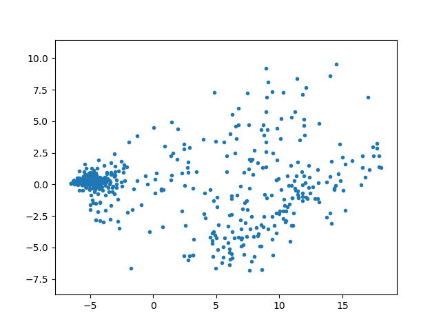
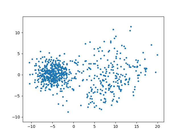
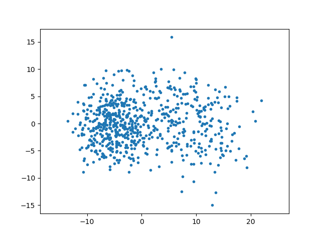
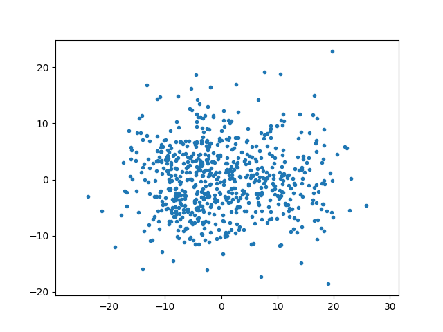
Dataset Comparison of seven approached in cluster number prediction CH Jump Hartigan Curvature Silhouette Gap $CV_{a}$ CNAK breast-cancer (3I) 2 2 13 2 2 5 2 2 breast-cancer (10I) 2 2 15 2 2 2 2 2 breast-cancer (30I) 2 2 15 2 2 2 2 2

Table 19: Clustering results on noisy breast-cancer dataset

Dataset Methods ARI NMI Homogeneity Completeness Silhouette Mode SM Mode SM Mode SM Mode SM Mode SM breast -cancer (3I) CNAK 0.84 0.84 0.74 0.74 0.73 0.73 0.75 0.75 0.42 0.42 BA 0.83 0.83 0.73 0.73 0.73 0.73 0.74 0.74 0.62 0.62 RS 0.83 0.83 0.73 0.73 0.73 0.73 0.74 0.74 0.62 0.62 RPKM 0.71 0.66 0.62 0.56 0.61 0.54 0.60 0.58 0.49 0.47 breast -cancer (10I) CNAK 0.79 0.78 0.67 0.67 0.67 0.67 0.67 0.68 0.27 0.27 BA 0.76 0.75 0.63 0.63 0.63 0.63 0.64 0.63 0.52 0.51 RS 0.75 0.75 0.63 0.63 0.63 0.63 0.63 0.63 0.51 0.51 RPKM 0.72 0.67 0.62 0.56 0.55 0.54 0.61 0.56 0.40 0.39 breast -cancer (30I) CNAK 0.56 0.56 0.43 0.44 0.44 0.44 0.43 0.44 0.16 0.16 BA 0.49 0.48 0.37 0.37 0.38 0.38 0.37 0.37 0.32 0.31 RS 0.49 0.49 0.37 0.37 0.38 0.38 0.37 0.37 0.32 0.32 RPKM 0.36 0.27 0.25 0.18 0.25 0.18 0.25 0.18 0.12 0.11

6 Conclusion

In this paper, we propose a novel cluster number assisted k-means (CNAK) algorithm. The proposed method consists of two steps. Initially, the number of clusters is estimated. In the second step, the clustering of data points is obtained. Automation in the determination of the cluster number determination is a major improvement in our work. In this paper, we investigate the applicability of our proposed work to handle a large scale dataset in an increasing number of instances as well as increasing dimensions. We study a few pertinent issues related to clustering. We design many simulations to discuss those issues. Our investigation reveals that the CNAK can predict a single cluster as well as multiple clusters. We find CNAK is robust against cluster imbalance as suggested by the results of clustering on sim-4. Moreover, it is efficient in handling a large scale dataset. But, its performance declines when the “between-cluster separation” is small. Also, it is unable to detect any shape clusters. Though it can indicate the existing hierarchical structure via a detailed analysis of the plot of “k vs. score”, the performance of clustering decreases with the increase in the depth of the hierarchy. The proposed algorithm CNAK is a Monte-Carlo simulation based method. Hence, determination of the size of a sampled dataset is a very crucial step and a key factor for the successful performance of the algorithm. However, with small scale data, we may work with a sample size of a higher fraction of dataset. But, this is not applicable, when the size of dataset becomes very large. We have proposed a heuristic to determine the size of a sampled dataset for a given dataset whose prediction for large scale dataset is feasible. The drop in computational time for the large dataset is governed by the small size of the sampled dataset in our proposed method. However, we observed that our heuristic fails when the dataset contains many clusters. In the future, we intend to apply our algorithm on a real-world, large-scale dataset for data mining.

7 Acknowledgments

This research did not receive any specific grant from funding agencies in the public, commercial, or not-for-profit sectors.

8 References

References

- Arthur & Vassilvitskii [2007] Arthur, D., & Vassilvitskii, S. (2007). K-means++: The Advantages of Careful Seeding. In Symposium on Discrete Algorithms (pp. 1027–1035). SIAM.
- Bradley & Fayyad [1998] Bradley, P. S., & Fayyad, U. M. (1998). Refining Initial Points for K-Means Clustering. In International Conference on Machine Learning (pp. 91–99). Morgan Kaufmann Publishers Inc.
- Calinski & Harabasz [1974] Calinski, T., & Harabasz, J. (1974). A dendrite method for cluster analysis. Communications in Statistics, 3, 1–27.
- Capo et al. [2017] Capo, M., Pérez, A., & Lozano, J. A. (2017). An efficient approximation to the K-means clustering for massive data. Knowledge-Based Systems, 117, 56–69.
- Chang & Yeung [2008] Chang, H., & Yeung, D.-Y. (2008). Robust path-based spectral clustering. Pattern Recognition, 41, 191 – 203.
- Chiang & Mirkin [2010] Chiang, M. M.-T., & Mirkin, B. (2010). Intelligent choice of the number of clusters in k-means clustering: An experimental study with different cluster spreads. Journal of Classification, 27, 3–40.
- Davidson & Satyanarayana [2003] Davidson, I., & Satyanarayana, A. (2003). Speeding up k-means Clustering by Bootstrap Averaging. In ICDM Workshop on Clustering Large Data Sets (pp. 16–25). IEEE.
- Davies & Bouldin [1979] Davies, D. L., & Bouldin, D. W. (1979). A Cluster Separation Measure. Transactions on Pattern Analysis and Machine Intelligence, 1, 224–227.
- Dheeru & Karra Taniskidou [2017] Dheeru, D., & Karra Taniskidou, E. (2017). UCI Machine Learning Repository.
- Dudoit & Fridlyand [2002] Dudoit, S., & Fridlyand, J. (2002). A prediction-based resampling method for estimating the number of clusters in a dataset. Genome biology, 3.
- Edmonds & Karp [1972] Edmonds, J., & Karp, R. M. (1972). Theoretical improvements in algorithmic efficiency for network flow problems. J. ACM, 19, 248–264.
- Ester et al. [1996] Ester, M., Kriegel, H.-P., Sander, J., & Xu, X. (1996). A Density-based Algorithm for Discovering Clusters a Density-based Algorithm for Discovering Clusters in Large Spatial Databases with Noise. In International Conference on Knowledge Discovery and Data Mining (pp. 226–231). AAAI Press.
- Estiri et al. [2018] Estiri, H., Omran, B. A., & Murphy, S. N. (2018). kluster: An efficient scalable procedure for approximating the number of clusters in unsupervised learning. Big Data Research, 13, 38 – 51.
- Fang & Wang [2012] Fang, Y., & Wang, J. (2012). Selection of the number of clusters via the bootstrap method. Computational Statistics & Data Analysis, 56, 468 – 477.
- Fränti et al. [2006] Fränti, P., Virmajoki, O., & Hautamäki, V. (2006). Fast agglomerative clustering using a k-nearest neighbor graph. IEEE Trans. on Pattern Analysis and Machine Intelligence, 28, 1875–1881.
- Fu & Medico [2007] Fu, L., & Medico, E. (2007). Flame, a novel fuzzy clustering method for the analysis of dna microarray data. BMC Bioinformatics, 8, 3.
- Gionis et al. [2007] Gionis, A., Mannila, H., & Tsaparas, P. (2007). Clustering aggregation. ACM Trans. Knowl. Discov. Data, 1.
- Gupta et al. [2018] Gupta, A., Datta, S., & Das, S. (2018). Fast automatic estimation of the number of clusters from the minimum inter-center distance for k-means clustering. Pattern Recognition Letters, 116, 72 – 79.
- Hancer & Karaboga [2017] Hancer, E., & Karaboga, D. (2017). A comprehensive survey of traditional, merge-split and evolutionary approaches proposed for determination of cluster number. Swarm and Evolutionary Computation, 32, 49 – 67.
- Hartigan [1975] Hartigan, J. A. (1975). Clustering Algorithms. (99th ed.). John Wiley & Sons, Inc.
- Hinneburg & Keim [1998] Hinneburg, A., & Keim, D. A. (1998). An Efficient Approach to Clustering in Large Multimedia Databases with Noise. In International Conference on Knowledge Discovery and Data Mining (pp. 58–65). AAAI Press.
- Horibe [1985] Horibe, Y. (1985). Entropy and correlation. IEEE Transactions on Systems, Man, and Cybernetics, SMC-15, 641–642.
- Hubert & Arabie [1985] Hubert, L., & Arabie, P. (1985). Comparing partitions. Journal of Classification, 2, 193–218.
- Jain & Law [2005] Jain, A. K., & Law, M. H. C. (2005). Data clustering: A user’s dilemma. In S. K. Pal, S. Bandyopadhyay, & S. Biswas (Eds.), Pattern Recognition and Machine Intelligence (pp. 1–10).
- Jr. [1963] Jr., J. H. W. (1963). Hierarchical grouping to optimize an objective function. Journal of the American Statistical Association, 58, 236–244.
- Lloyd [1982] Lloyd, S. (1982). Least squares quantization in PCM. Transactions on Information Theory, 28, 129–137.
- Ng et al. [2001] Ng, A. Y., Jordan, M. I., & Weiss, Y. (2001). On spectral clustering: Analysis and an algorithm. In ADVANCES IN NEURAL INFORMATION PROCESSING SYSTEMS (pp. 849–856). MIT Press.
- Rezaei & Fränti [2016] Rezaei, M., & Fränti, P. (2016). Set-matching methods for external cluster validity. IEEE Trans. on Knowledge and Data Engineering, 28, 2173–2186.
- Rosenberg & Hirschberg [2007] Rosenberg, A., & Hirschberg, J. (2007). V-Measure: A Conditional Entropy-Based External Cluster Evaluation Measure. In Joint Conference on Empirical Methods in Natural Language Processing and Computational Natural Language Learning (pp. 410–420).
- Rousseeuw [1987] Rousseeuw, P. J. (1987). Silhouettes: A graphical aid to the interpretation and validation of cluster analysis. Journal of Computational and Applied Mathematics, 20, 53–65.
- Sugar & James [2003] Sugar, C. A., & James, G. M. (2003). Finding the Number of Clusters in a Dataset: An Information-Theoretic Approach. Journal of the American Statistical Association, 98, 750–763.
- Tibshirani et al. [2001] Tibshirani, R., Walther, G., & Hastie, T. (2001). Estimating the number of clusters in a data set via the gap statistic. Journal of the Royal Statistical Society: Series B (Statistical Methodology), 63, 411–423.
- Tryfos [2009] Tryfos, P. (2009). Simple random samples and their properties. Technical Report University of York.
- Veenman et al. [2002] Veenman, C. J., Reinders, M. J. T., & Backer, E. (2002). A maximum variance cluster algorithm. IEEE Transactions on Pattern Analysis and Machine Intelligence, 24, 1273–1280.
- Wang [2010] Wang, J. (2010). Consistent selection of the number of clusters via crossvalidation. Biometrika, 97, 893–904.
- Xu et al. [1998] Xu, X., Ester, M., Kriegel, H. P., & Sander, J. (1998). A distribution-based clustering algorithm for mining in large spatial databases. In International Conference on Data Engineering (pp. 324–331). IEEE.
- Zahn [1971] Zahn, C. T. (1971). Graph-theoretical methods for detecting and describing gestalt clusters. IEEE Transactions on Computers, C-20, 68–86.
- Zhang et al. [2017] Zhang, Y., Mańdziuk, J., Quek, C. H., & Goh, B. W. (2017). Curvature-based method for determining the number of clusters. Information Sciences, 415-416, 414–428.
- del Águila & González-Ramírez [2014] del Águila, M. R., & González-Ramírez, A. (2014). Sample size calculation. Allergologia et Immunopathologia, 42, 485 – 492.