A Fast Sampling Gradient Tree Boosting Framework

Abstract

As an adaptive, interpretable, robust, and accurate meta-algorithm for arbitrary differentiable loss functions, gradient tree boosting is one of the most popular machine learning techniques, though the computational expensiveness severely limits its usage. Stochastic gradient boosting could be adopted to accelerates gradient boosting by uniformly sampling training instances, but its estimator could introduce a high variance. This situation arises motivation for us to optimize gradient tree boosting. We combine gradient tree boosting with importance sampling, which achieves better performance by reducing the stochastic variance. Furthermore, we use a regularizer to improve the diagonal approximation in the Newton step of gradient boosting. The theoretical analysis supports that our strategies achieve a linear convergence rate on logistic loss. Empirical results show that our algorithm achieves a 2.5x–18x acceleration on two different gradient boosting algorithms (LogitBoost and LambdaMART) without appreciable performance loss.

1 Introduction

Gradient tree boosting [Friedman, 2001] is a proven technique for both classification and regression problems. Comparing to other techniques, it achieves a higher accuracy while consuming more computation resources. Figure 1 shows that LambdaMART (a gradient tree boosting algorithm) fulfils higher accuracy but costs much longer time among several machine-learned ranking algorithms.

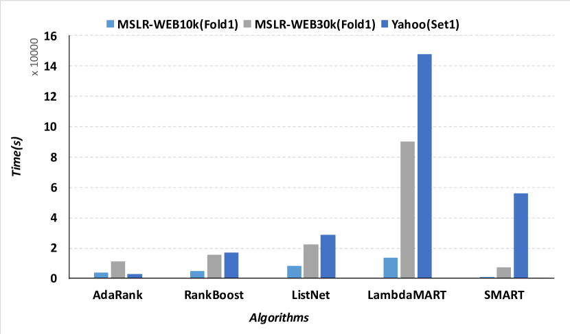
(a) Efficiency

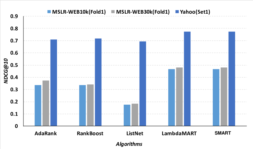
(b) Accuracy (NDCG@10)

Figure 1: Performance of different ranking algorithms. Results of AdaRank, RankBoost, and ListNet are tested on RankLib [Dang, 2013]; LambdaMART is implemented by us according to [Burges, 2010].

Previous work such as [Appel et al., 2013, Dubout and Fleuret, 2014, Johnson and Zhang, 2014, Kalal et al., 2008, Needell et al., 2014] has been done to accelerate gradient boosting. In this paper, we propose a sampling framework named SMART (Sampling Multiple Additive Regression Tree) that accelerates gradient tree boosting through the following two methods.

Importance sampling

Stochastic gradient boosting [Friedman, 2002] was extensively utilized to accelerate gradient boosting algorithms. This technique uniformly samples training instances, which guarantees the sampled dataset being an unbiased estimation of the original dataset. However, the variance of the stochastic gradient estimator could be high since the stochastic gradient varies significantly over different instances. As [Zhao and Zhang, 2015] demonstrated, the variance is minimized when sampling probability is roughly proportional to the norm of the gradient. In SMART, sampling probability is roughly proportional to the first/second-order gradient of training instances, which leads to satisfactory performance in our experiments.

Improved diagonal approximation

XGBoost [Chen and Guestrin, 2016] uses the diagonal approximation on the Hessian in its Newton step, where non-diagonal elements in the Hessian matrix are abandoned. Such approximation has a remarkable negative impact on the algorithm. However, veritably computing the whole Hessian matrix and its inverse is computationally unfeasible. Inspired by [Shamir et al., 2014], we put a regularizer on the loss function, so the non-diagonal elements in the Hessian matrix are filled in an approximate manner.

Details of the algorithms are listed in §3. To guarantee the effectiveness of the algorithms, theoretical and experimental support are given in §4 and §5, respectively. We summarize our contribution as follows:

1. We demonstrate a universal framework SMART, which is driven by importance sampling and improved diagonal approximation, that accelerates all gradient tree boosting algorithms;

2. We proved that gradient tree boosting combined with importance sampling and logistic loss achieves a linear convergence rate;

3. We implemented SMART upon LogitBoost and LambdaMART; our implementation achieves ideal efficiency and accuracy (2.5x–18x acceleration without appreciable accuracy loss) on multiple real-world datasets, which is superior to stochastic gradient boosting and weight trimming.

2 Related Work

2.1 Gradient Tree Boosting

Gradient tree boosting [Friedman, 2001] produces an ensemble of regression trees as the prediction model. XGBoost [Chen and Guestrin, 2016] improved the algorithm by introducing Newton’s method in function space. It optimizes arbitrary second-order differentiable loss function by fit the regression tree to Newton’s step. Details are listed in algorithm 1.

Algorithm 1 Gradient tree boosting

   $\bm{y}\leftarrow\bm{0}$

  for all iteration $t$ do

     for all instance $i$ do

        $g_{i}\leftarrow\partial\ell/\partial\hat{y}_{i}$

        $h_{i}\leftarrow\partial^{2}\ell/\partial\hat{y}_{i}^{2}$

     end for

     fit $f$ to the Newton’s step $-\bm{g}/\bm{h}$ with diagonal approximation

      $\bm{y}\leftarrow\bm{y}+\nu f(\bm{X})$

  end for

  return   all decision trees

2.2 LogitBoost

LogitBoost [Friedman et al., 2000] solves the binary classification problem by applying the logistic loss function to gradient boosting, where the loss function is

$$\ell(\hat{y}_{i})=y_{i}\ln\frac{1}{\psi_{i}}+(1-y_{i})\ln\frac{1}{1-\psi_{i}},$$

and the binary label $y_{i}\in\{0,1\}$, $\psi_{i}$ is the probability of label being positive

$$\psi_{i}=\Pr(y_{i}=1)=\frac{e^{\hat{y}_{i}}}{e^{\hat{y}_{i}}+e^{-\hat{y}_{i}}}.$$

LogitBoost is the straightforward combination of algorithm 1 and the first & second gradient of the logistic loss

$$\bm{g}=\nabla\ell(\bm{\hat{y}})=2(\bm{\psi}-\bm{y}),$$

and

$$\bm{h}=\nabla^{2}\ell(\bm{\hat{y}})=4\langle\bm{\psi},1-\bm{\psi}\rangle.$$

2.3 LambdaMART

Learning to rank is a task to train a ranking model with machine learning techniques, such that the model sorts new instances according to their relevance, preference, or importance. Previous work has shown that LambdaMART [Burges, 2010] is an outperforming solution to the ranking problem, which championed the Yahoo! Learning to Rank Challenge [Chapelle and Chang, 2011]. LambdaMART is the algorithm combining gradient tree boosting and the following loss function

$$\ell(\bm{s})=\sum_{\{i,j\}\in I}|\Delta\text{NDCG}_{ij}|\log\left(1+e^{-\sigma(s_{i}-s_{j})}\right),$$

where $\bm{s}$ is the model output, $I$ is the set of preference pairs from the training data, and NDCG is an indicator measuring the quality of a permutation. From the above loss function we have

$$g_{i}=\frac{\partial\ell(\bm{s})}{\partial s_{i}}$$

$$=\sum_{j:\{i,j\}\in I}\frac{-\sigma|\Delta\text{NDCG}_{ij}|}{1+e^{\sigma(s_{i}-s_{j})}}+\sum_{j:\{j,i\}\in I}\frac{\sigma|\Delta\text{NDCG}_{ij}|}{1+e^{\sigma(s_{j}-s_{i})}},$$

and

$$h_{i}=\frac{\partial^{2}\ell(\bm{s})}{\partial s_{i}^{2}}$$

$$=\sum_{j:\{i,j\}\in I}\frac{\sigma^{2}|\Delta\text{NDCG}_{ij}|e^{\sigma(s_{i}-s_{j})}}{\left(1+e^{\sigma(s_{i}-s_{j})}\right)^{2}}$$

$$+\sum_{j:\{j,i\}\in I}\frac{\sigma^{2}|\Delta\text{NDCG}_{ij}|e^{\sigma(s_{j}-s_{i})}}{\left(1+e^{\sigma(s_{j}-s_{i})}\right)^{2}}.$$

LambdaMART is the straightforward combination of algorithm 1 and the above $g_{i}$, $h_{i}$.

2.4 Weight trimming

First introduced in [Friedman et al., 2000], weight trimming is an idea that correctly classified instances with high confidence, viz. instances with weight less than a certain threshold, should be abandoned in each boosting iteration. Friedman observed that the computation time was dramatically reduced while accuracy was not sacrificed.

2.5 Stochastic Gradient Boosting

[Friedman, 2002] proposed that a tree should be fit on a random subsample of the training set in each boosting iteration. Instead of abandoning instances with small weights, stochastic gradient boosting samples training instances uniformly, v.i.z. that whether each instance being sampled are i.i.d. Bernoulli variables. Friedman observed that the accuracy of gradient boosting was substantially improved.

3 Algorithms

SMART consists of two strategies, both of which accelerates arbitrary gradient tree boosting algorithms with a second-order differentiable loss function. The first strategy is the gradient boosting with Newton’s method combined with importance sampling, where the importance is defined as the first gradient. The second strategy is the gradient boosting with Newton’s method combined with importance sampling and improved diagonal approximation, where the importance is defined as the second gradient.

3.1 First-gradient-proportional sampling

In the regression tree construction procedure, all instances are enumerated several times in each boosting step. It is reasonable to use a subsample of instances to construct each regression tree. In this algorithm, we introduce importance sampling into gradient boosting, which is superior to uniform sampling by achieving lower variance. In the same way as [Friedman, 2002] did, we make independent decision to sample each instance on each iteration. Furthermore, we define Bernoulli variable $q_{i}^{(t)}\in\{0,1\}$ indicating whether $i^{\text{th}}$ instance is utilized on $t^{\text{th}}$ iteration, and $p_{i}^{(t)}=\Pr\left(q_{i}^{(t)}=1\right)$ being the sampling probability.

Differing from [Friedman, 2002], $\{q_{i}\}_{1}^{N}$ are not i.i.d. Bernoulli variables. As [Zhao and Zhang, 2015] demonstrated, the variance of the gradient estimator is minimized when the sampling probability is roughly proportional to the norm of the gradient, such that

$$p_{i}=\min(1,\rho|g_{i}|),$$

where $\rho$ is a tuning parameter.

In order to eliminate the bias of the empirical risk introduced by the sampling algorithm, the regression tree is constructed upon the importance-balanced loss function of

$$\operatorname*{arg\,min}_{f}\sum_{i=0}^{n}\frac{q_{i}}{p_{i}}\ell(f(\bm{x}_{i})).$$

First and second gradient is derived from this loss function such that $\tilde{g}_{i}=\frac{q_{i}}{p_{i}}g_{i}$ and $\tilde{h}_{i}=\frac{q_{i}}{p_{i}}h_{i}$. This algorithm is listed in algorithm 2.

Algorithm 2 First-gradient-proportional sampling

  $\bm{y}\leftarrow\bm{0}$

  for all iteration $t$ do

     for all instance $i\in\{1\dots n\}$ do

        $g_{i}\leftarrow\partial\ell/\partial y_{i}$

        $h_{i}\leftarrow\partial^{2}\ell/\partial y_{i}^{2}$

        $p_{i}\leftarrow\min(1,\rho|g_{i}|)$

        generate value $q_{i}\in\{0,1\}$ by Bernoulli parameter $p_{i}$

        $g_{i}\leftarrow\frac{q_{i}}{p_{i}}g_{i}$

        $h_{i}\leftarrow\frac{q_{i}}{p_{i}}h_{i}$

     end for

     fit $f$ to the Newton’s step $f(\bm{x}_{i})=-g_{i}/h_{i}$ from the subset $\mathcal{S}=\{i|q_{i}=1\}$

     $\bm{y}\leftarrow\bm{y}+\nu f(\bm{X})$

  end for

  return  all decision trees

3.2 Second-gradient-proportional sampling

XGBoost [Chen and Guestrin, 2016] introduced Newton’s method into gradient boosting, which accelerates the algorithm dramatically. However, non-diagonal elements in the Hessian matrix are abandoned in Newton’s step. Such approximation gives a negative impact on the algorithm. [Shamir et al., 2014] demonstrated that by solving the problem

$$\operatorname*{arg\,min}_{f}\sum_{i=1}^{n}\left(\ell(\tilde{y}_{i})+\langle\ell^{\prime}(\tilde{y}),f(\bm{x}_{i})-\tilde{y}_{i}\rangle+\frac{1}{\eta}D(f(\bm{x}_{i}),\tilde{y}_{i})\right)$$ (1)

with Newton’s method, we get a more accurate Newton’s step, although the Hessian matrix is not entirely computed. In equation 1, the $\tilde{y}_{i}$ is a rough estimation of $y_{i}$. Specifically, it is the the hypothesis of last two iterations in our implementation. $\ell^{\prime}(\tilde{y})$ is defined as

$$\ell^{\prime}(\tilde{y})=\frac{1}{|I_{j}|}\sum_{\imath\in I_{j}}\ell^{\prime}(\tilde{y}_{\imath}),$$

where $I_{j}$ is the instance set of the regression tree leaf $j$ which covers instance $i$. $D(\cdot,\cdot)$ is the Bregman divergence corresponding to the loss function $\ell(\cdot)$

$$D(f(\bm{x}_{i}),\tilde{y}_{i})=\ell(f(\bm{x}_{i}))-\ell(\tilde{y}_{i})-\langle\ell^{\prime}(\tilde{y}_{i}),f(\bm{x}_{i})-\tilde{y}_{i}\rangle.$$

Plugging $\ell^{\prime}(\tilde{y})$ and $D(f(\bm{x}_{i}),\tilde{y}_{i})$ into 1, eliminating constant items, we have

$$\operatorname*{arg\,min}_{f}\left(\ell(f(\bm{x}_{i}))-\ell^{\prime}(\tilde{y}_{i})f(\bm{x}_{i})+\frac{\eta f(\bm{x}_{i})}{|I_{j}|}\sum_{\imath\in I_{j}}\ell^{\prime}(\tilde{y}_{\imath})\right).$$

Applying importance balancing to eliminate the bias, we have the final loss function

$$L(f(\bm{X}))=\frac{q_{i}}{p_{i}}\left(\ell(f(\bm{x}_{i}))-\ell^{\prime}(\tilde{y}_{i})f(\bm{x}_{i})+\frac{\eta f(\bm{x}_{i})}{|I_{j}|}\sum_{\imath\in I_{j}}\ell^{\prime}(\tilde{y}_{\imath})\right).$$

From this loss function, we have the first and second gradient for Newton’s step

$$\tilde{g}_{i}=\frac{q_{i}}{p_{i}}\left(g_{i}-\ell^{\prime}(\tilde{y}_{i})+\frac{\eta}{|I_{j}|}\sum_{\imath\in I_{j}}\ell^{\prime}(\tilde{y}_{\imath})\right),$$

and

$$\tilde{h}_{i}=\frac{q_{i}}{p_{i}}h_{i}.$$

In this algorithm, the sampling probability is roughly proportional to the second gradient such that $p_{i}=\min(1,\rho h_{i})$.

Algorithm 3 Second-gradient-proportional sampling

  $\bm{y}\leftarrow\bm{0}$

  for all iteration $t$ do

     for all instance $i\in\{1\dots n\}$ do

        $g_{i}\leftarrow\partial\ell/\partial y_{i}$

        $h_{i}\leftarrow\partial^{2}\ell/\partial y_{i}^{2}$

        $p_{i}\leftarrow\min(1,\rho h_{i})$

        generate value $q_{i}\in\{0,1\}$ by Bernoulli parameter $p_{i}$

        $g_{i}\leftarrow\frac{q_{i}}{p_{i}}\left(g_{i}-\ell^{\prime}(\tilde{y}_{i})+\eta\ell^{\prime}(\tilde{y})\right)$

        $h_{i}\leftarrow\frac{q_{i}}{p_{i}}h_{i}$

     end for

     fit $f$ to the Newton’s step $f(\bm{x}_{i})=-g_{i}/h_{i}$ from the subset $\mathcal{S}=\{i|q_{i}=1\}$

     $\bm{y}\leftarrow\bm{y}+\nu f(\bm{X})$

  end for

  return  all decision trees

4 Analysis

In this section, we provide a theoretical guarantee that our first-gradient-proportional subsampling achieves a linear convergence rate over the logistic loss. Before presenting the result, we give some definitions as follows.

1. Let $\bm{V}\in\mathbb{R}^{N\times J}$ encoding the tree structure which transforms instances to leaf nodes, such that $v_{ij}=1$ if the $i^{\text{th}}$ instance sinks into the $j^{\text{th}}$ leaf, and $0$ otherwise.

2. Let $\bm{Q}=\mathrm{diag}\left(\begin{smallmatrix}\frac{q_{1}}{p_{1}}&\cdots&\frac{q_{N}}{p_{N}}\end{smallmatrix}\right)$.

Under such definitions, Newton’s step of the legacy gradient tree boosting is

$$\bm{f}=-\nu\bm{V}(\bm{V}^{\mkern-1.5mu\mathsf{T}}\bm{H}\bm{V})^{-1}\bm{V}^{\mkern-1.5mu\mathsf{T}}\bm{g},$$

and of the first-gradient-proportional subsampling algorithm is

$$\bm{f}=-\nu\bm{V}(\bm{V}^{\mkern-1.5mu\mathsf{T}}\bm{H}\bm{Q}\bm{V})^{-1}\bm{V}^{\mkern-1.5mu\mathsf{T}}\bm{Q}\bm{g}.$$

such that $\bm{y}^{+}=\bm{y}+\bm{f}$, where $\bm{y}^{+}$ is the prediction after another boosting iteration. The linear convergence rate is established upon the following two theorems.

Theorem 4.1.

Given a sequence $\epsilon_{0}>\epsilon_{1}>\cdots>\epsilon_{T}>0$ with the recurrence relation $\epsilon_{t+1}\leq\gamma\epsilon_{t}$ where $\gamma\in(0,1)$ is a small constant, we have a linear convergence that

$$\epsilon_{T}<\epsilon_{0}\gamma^{T}.$$

Theorem 4.2.

Given that

$$\bm{f}=-\nu\bm{V}(\bm{V}^{\mkern-1.5mu\mathsf{T}}\bm{H}\bm{Q}\bm{V})^{-1}\bm{V}^{\mkern-1.5mu\mathsf{T}}\bm{Q}\bm{g},$$

we have

$$L\left(\bm{y}^{+}\right)=L(\bm{y}+\bm{f})\leq\gamma L(\bm{y}),$$

where $0<\gamma<1$.

Theorem 4.1 is self-evident and its proof is omitted here. The proof for theorem 4.2 is given in appendix A.

5 Experiments

We implement SMART upon two gradient tree boosting algorithms, LogitBoost and LambdaMART, each with two subsampling strategies. Multiple real-world datasets are employed to verify the efficiency of SMART.

LogitBoost is tested on the LIBSVM/a8a datasets [Chang and Lin, 2011]; LambdaMART is tested on three large-scale datasets: MSLR-WEB10K/MSLR-WEB30K of LETOR datasets [Qin and Liu, 2013], and Yahoo! Learning to Rank Challenge dataset [Chapelle and Chang, 2011]. Principal characteristics of these datasets are given in table 1. Note that a8a is a binary classification dataset, while the others are ranking datasets.

Table 1: Properties of Datasets

dataset	#train	#test	#dim
LIBSVM/a8a	22696	9865	123
MSLR-WEB10K/Fold1	719311	241521	136
MSLR-WEB30K/Fold1	2258066	753611	136
Yahoo/Set1	466687	165660	700

SMART is compared with 1) legacy LogitBoost or LambdaMART without any instance selecting strategies as the baseline, 2) weight-trimming, and 3) stochastic gradient boosting (uniform subsampling).

Results are shown in figure 2, 4, 6, and 8, from which we can tell that 1) second-gradient-proportional strategy utilizes the least training instances when it converges to its ideal accuracy; and 2) as boosting iteration proceeds, second-gradient-proportional strategy achieves much better accuracy than (or almost same accuracy with) the baseline.

Each of table 2, 4, 6, 8 consists of two parts. The upper part shows the performance details when each algorithm achieves a relatively ideal accuracy; the lower part shows the details when each algorithm achieves their best accuracy. Take MSLR-WEB10K for example, when it achieves an NDCG@10 at 0.453, the second-gradient-proportional subsampling strategy takes 54 iterations and averagely utilizes 6% training instances in each iteration; when it achieves an NDCG@10 at 0.465, the second-gradient-proportional subsampling strategy only takes 730 seconds, which achieves an 18x acceleration.

In conclusion, our second-gradient-proportional subsampling strategy precisely portrays the characteristics of the original dataset while consumes the least sample size. Taking efficiency and accuracy into account, the second-gradient-proportional subsampling strategy is superior to any other algorithms in our experiments.

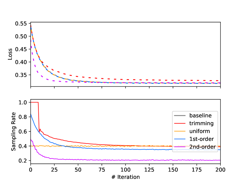
Figure 2: Loss curve on a8a

	loss	iter	ASRI	time/s
baseline	0.325	60	1.0000	65
uniform	0.325	58	0.3998	16
trimming	0.325	443	0.4195	141
1st-order	0.325	57	0.5028	15
2nd-order	0.325	34	0.3052	6
baseline	0.319	97	1.0000	127
uniform	0.319	96	0.3993	24
trimming	0.325	443	0.4195	141
1st-order	0.319	89	0.4531	22
2nd-order	0.319	142	0.2317	20

Table 2: Performance on a8a

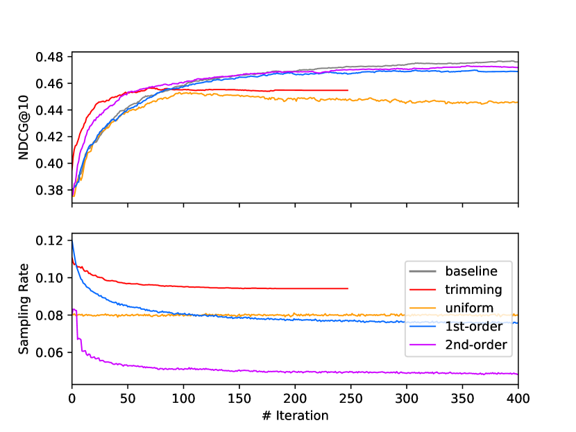
Figure 3: NDCG curve on MSLR-WEB10K

	NDCG	iter	ASRI	time/s
baseline	0.453	83	1.0000	6899
uniform	0.453	100	0.0799	779
trimming	0.453	52	0.1018	403
1st-order	0.453	83	0.0902	665
2nd-order	0.453	54	0.0604	273
baseline	0.465	141	1.0000	13190
uniform	0.453	100	0.0799	779
trimming	0.456	72	0.1004	571
1st-order	0.465	162	0.0851	1349
2nd-order	0.465	138	0.0549	730

Figure 4: Performance on MSLR-WEB10K

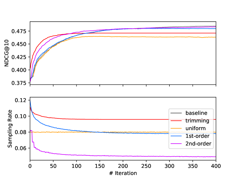
Figure 5: NDCG curve on MSLR-WEB30K

	NDCG	iter	ASRI	time/s
baseline	0.464	97	1.0000	33773
uniform	0.464	117	0.0800	6495
trimming	0.464	47	0.1021	2948
loss-based	0.464	95	0.1468	7453
1st-order	0.464	94	0.0901	5652
2nd-order	0.464	63	0.0595	1654
baseline	0.480	228	1.0000	89898
uniform	0.464	117	0.0800	6495
trimming	0.471	139	0.0984	9405
1st-order	0.480	247	0.0836	16234
2nd-order	0.480	236	0.0530	6827

Figure 6: Performance on MSLR-WEB30K

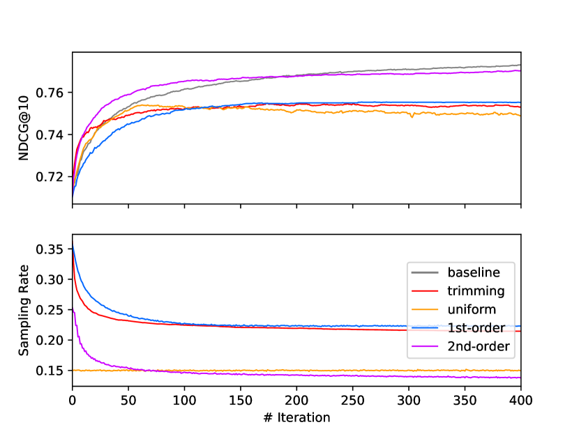
Figure 7: NDCG curve on Yahoo! dataset

	NDCG	iter	ASRI	time/s
baseline	0.754	57	1.0000	18200
uniform	0.754	66	0.1500	2623
trimming	0.754	169	0.2352	10156
1st-order	0.754	147	0.2455	11389
2nd-order	0.754	35	0.1804	1769
baseline	0.772	357	1.0000	147872
uniform	0.754	66	0.1500	2623
trimming	0.755	632	0.2201	35355
1st-order	0.755	173	0.2423	14118
2nd-order	0.772	645	0.1430	55651

Figure 8: Performance on Yahoo! dataset

6 Conclusion

In this paper, we presented SMART, an efficient subsampling framework based on gradient tree boosting. Inspired by [Zhao and Zhang, 2015], we introduced importance sampling such that subsampling probability is roughly proportional to the gradient. Inspired by [Shamir et al., 2014], we fill the Hessian matrix in an approximate manner. Theoretically, we proved that SMART achieves a linear convergence rate on logistic loss, which is same as the legacy LogitBoost. Practically, we implemented SMART upon LogitBoost and LambdaMART. Experiments show that our implementation achieves a 2.5x–18x acceleration under real-world, large-scale datasets.

Furthermore, SMART could be applied on more gradient boosting algorithms, such as AdaBoost, for further guarantee.

Appendix A Proof of theorem 4.2

Following auxiliary lemmas are needed to prove theorem 4.2.

Lemma A.1.

$(\bm{V}^{\mkern-1.5mu\mathsf{T}}\bm{H}_{\bm{\xi}}\bm{Q}\bm{V})(\bm{V}^{\mkern-1.5mu\mathsf{T}}\bm{H}\bm{Q}\bm{V})^{-1}\leq\mu\bm{I}$, where $\bm{H}_{\bm{\xi}}=\mathrm{diag}(\begin{smallmatrix}\ell^{\prime\prime}(\xi_{1})&\dots&\ell^{\prime\prime}(\xi_{N})\end{smallmatrix})$.

Proof.

[Sun et al., 2014]’s lemma 9 proved that

$$\frac{\ell^{\prime\prime}(\xi)}{\ell^{\prime\prime}(y)}\leq e^{2|\xi-y|},$$

which gives

$$\sum_{i\in I_{j}}\frac{q_{i}\ell^{\prime\prime}(\xi_{i})}{p_{i}}\leq\sum_{i\in I_{j}}\frac{q_{i}\ell^{\prime\prime}(y_{i})e^{2|\xi_{i}-y_{i}|}}{p_{i}},$$

which is equivalent to

$$(\bm{V}^{\mkern-1.5mu\mathsf{T}}\bm{H}_{\bm{\xi}}\bm{Q}\bm{V})(\bm{V}^{\mkern-1.5mu\mathsf{T}}\bm{H}\bm{Q}\bm{V})^{-1}\leq\exp(\max_{i}|\xi_{i}-y_{i}|)\bm{I}.$$

∎

Lemma A.2.

$\bm{g}^{\mkern-1.5mu\mathsf{T}}\bm{Q}\bm{V}(\bm{V}^{\mkern-1.5mu\mathsf{T}}\bm{H}\bm{Q}\bm{V})^{-1}\bm{V}^{\mkern-1.5mu\mathsf{T}}\bm{Q}\bm{g}\leq\gamma^{2}\bm{g}^{\mkern-1.5mu\mathsf{T}}\bm{Q}(\bm{H}\bm{Q})^{-1}\bm{Q}\bm{g}$.

Proof.

Recall that $\ell(y)=-r\ln\psi-(1-r)\ln(1-\psi)$, and $\psi=\frac{e^{y}}{e^{y}+e^{-y}}$, which yield $\frac{\mathop{}\!\mathrm{d}\psi}{\mathop{}\!\mathrm{d}y}=2\psi(1-\psi)$, $g=\ell^{\prime}(y)=2(\psi-r)$, and $h=\ell^{\prime\prime}(y)=4\psi(1-\psi)$. Defining $\phi=|r-\psi|$, we have $g^{2}=4\phi^{2}$, $h=4\phi(1-\phi)$, and $\frac{g^{2}}{h}=\frac{\phi}{1-\phi}$. The $\psi_{i}$ clapping yields $\frac{1}{1-\phi_{i}}\leq\frac{1}{\rho}$, and $1-\phi_{i}\leq 1$. We have

$$\left(\sum_{i\in I_{j}}\frac{q_{i}h_{i}}{p_{i}}\right)\left(\sum_{i\in I_{j}}\frac{q_{i}g_{i}^{2}}{p_{i}h_{i}}\right)$$

$$= \left(\sum_{i\in I_{j}}\frac{4q_{i}\phi_{i}(1-\phi_{i})}{p_{i}}\right)\left(\sum_{i\in I_{j}}\frac{q_{i}\phi_{i}}{p_{i}(1-\phi_{i})}\right)$$

$$\leq \frac{4}{\rho}\left(\sum_{i\in I_{j}}\frac{q_{i}\phi_{i}}{p_{i}}\right)\left(\sum_{i\in I_{j}}\frac{q_{i}\phi_{i}}{p_{i}}\right)$$

$$\leq \frac{4n_{j}}{\rho}\sum_{i\in I_{j}}\left(\frac{q_{i}\phi_{i}}{p_{i}}\right)^{2}$$

$$= \frac{n_{j}}{\rho}\sum_{i\in I_{j}}\left(\frac{q_{i}g_{i}}{p_{i}}\right)^{2}.$$ (2)

We perform a weak learnability assumption here such that for some $\delta>0$ we have

$$\left(\sum_{i\in I_{j}}\frac{q_{i}g_{i}}{p_{i}}\right)^{2}\geq 4\delta^{2}\sum_{i\in I_{j}}\left(\frac{q_{i}g_{i}}{p_{i}}\right)^{2}.$$ (3)

Combining (2) and (3), it yields

$$\left(\sum_{i\in I_{j}}\frac{q_{i}g_{i}}{p_{i}}\right)^{2}\left(\sum_{i\in I_{j}}\frac{q_{i}h_{i}}{p_{i}}\right)^{-1}\geq\frac{4\delta^{2}\rho}{n_{j}}\left(\sum_{i\in I_{j}}\frac{q_{i}g_{i}^{2}}{p_{i}h_{i}}\right),$$

which completes this proof. ∎

Lemma A.3.

$\bm{g}^{\mkern-1.5mu\mathsf{T}}\bm{Q}(\bm{H}\bm{Q})^{-1}\bm{Q}\bm{g}\leq\sum\frac{q_{i}}{p_{i}}\ell(y_{i})$.

Proof.

[Sun et al., 2014]’s theorem 4 proved $\frac{g_{i}^{2}}{h_{i}}\geq\ell(y_{i})$, which gives

$$\frac{\left(\frac{q_{i}g_{i}}{p_{i}}\right)^{2}}{\frac{q_{i}h_{i}}{p_{i}}}=\frac{q_{i}g_{i}^{2}}{p_{i}h_{i}}\geq\frac{q_{i}}{p_{i}}\ell(y_{i}),$$

completing this proof. ∎

Finally, we are now ready to prove theorem 4.2.

Proof.

Applying Taylor’s theorem on $L(\cdot)$ between $\bm{y}$ and $\bm{y}+\bm{f}$ yields

$$L(\bm{y}+\bm{f})$$

$$= L(\bm{y})+\nabla L(\bm{y})^{\mkern-1.5mu\mathsf{T}}\bm{f}+\frac{1}{2}\bm{f}^{\mkern-1.5mu\mathsf{T}}\nabla^{2}L(\bm{\xi})\bm{f}$$

$$= L(\bm{y})+\bm{g}^{\mkern-1.5mu\mathsf{T}}\bm{Q}\bm{f}+\frac{1}{2}\bm{f}^{\mkern-1.5mu\mathsf{T}}\bm{H}_{\bm{\xi}}\bm{Q}\bm{f},$$

where $\bm{\xi}$ is a vector between $\bm{y}$ and $\bm{y}+\bm{f}$. Replacing $\bm{f}$ with the given Newton step yields

$$L(\bm{y}+\bm{f})=L(\bm{y})-\nu\bm{g}^{\mkern-1.5mu\mathsf{T}}\bm{Q}\bm{V}(\bm{V}^{\mkern-1.5mu\mathsf{T}}\bm{H}\bm{Q}\bm{V})^{-1}\bm{V}^{\mkern-1.5mu\mathsf{T}}\bm{Q}\bm{g}$$

$$+\frac{\nu^{2}}{2}\bm{g}^{\mkern-1.5mu\mathsf{T}}\bm{Q}\bm{V}(\bm{V}^{\mkern-1.5mu\mathsf{T}}\bm{H}\bm{Q}\bm{V})^{-1}(\bm{V}^{\mkern-1.5mu\mathsf{T}}\bm{H}_{\bm{\xi}}\bm{Q}\bm{V})$$

$$(\bm{V}^{\mkern-1.5mu\mathsf{T}}\bm{H}\bm{Q}\bm{V})^{-1}\bm{V}^{\mkern-1.5mu\mathsf{T}}\bm{Q}\bm{g}.$$

Applying lemma A.1 yields

$$L(\bm{y}+\bm{f})\leq L(\bm{y})$$

$$+\left(\frac{\mu\nu^{2}}{2}-\nu\right)\bm{g}^{\mkern-1.5mu\mathsf{T}}\bm{Q}\bm{V}(\bm{V}^{\mkern-1.5mu\mathsf{T}}\bm{H}\bm{Q}\bm{V})^{-1}\bm{V}^{\mkern-1.5mu\mathsf{T}}\bm{Q}\bm{g}.$$

Applying lemma A.2 yields

$$L(\bm{y}+\bm{f})\leq L(\bm{y})+\gamma^{2}\left(\frac{\mu\nu^{2}}{2}-\nu\right)\bm{g}^{\mkern-1.5mu\mathsf{T}}\bm{Q}(\bm{H}\bm{Q})^{-1}\bm{Q}\bm{g}.$$

Applying lemma A.3 yields

$$L(\bm{y}+\bm{f})\leq\left[1-\gamma^{2}\left(\nu-\frac{\mu\nu^{2}}{2}\right)\right]L(\bm{y}).$$

By setting a proper shrinkage $\nu$ such that $0<\gamma^{2}\left(\nu-\frac{\mu\nu^{2}}{2}\right)<1$, a linear convergence rate can be established. ∎

References

- Appel et al. [2013] Ron Appel, Thomas J Fuchs, Piotr Dollár, and Pietro Perona. Quickly Boosting Decision Trees: Pruning Underachieving Features Early. In Proceedings of the 30th International Conference on Machine Learning, volume 28, pages 594–602, 2013.
- Burges [2010] Christopher J.C. Burges. From RankNet to LambdaRank to LambdaMART: An Overview. Technical report, Microsoft, 2010.
- Chang and Lin [2011] Chih-Chung Chang and Chih-Jen Lin. LIBSVM: A library for support vector machines. ACM Transactions on Intelligent Systems and Technology, 2:27:1–27:27, 2011. URL http://www.csie.ntu.edu.tw/~cjlin/libsvm.
- Chapelle and Chang [2011] Olivier Chapelle and Yi Chang. Yahoo! Learning to Rank Challenge Overview. JMLR: Workshop and Conference Proceedings, 14:1–24, 2011.
- Chen and Guestrin [2016] Tianqi Chen and Carlos Guestrin. XGBoost. In Proceedings of the 22nd ACM SIGKDD International Conference on Knowledge Discovery and Data Mining - KDD ’16, pages 785–794, New York, New York, USA, 2016. ACM Press. ISBN 9781450342322. doi: 10.1145/2939672.2939785.
- Dang [2013] V. Dang. RankLib, 2013. URL http://sourceforge.net/p/lemur/wiki/RankLib.
- Dubout and Fleuret [2014] Charles Dubout and François Fleuret. Adaptive Sampling for Large Scale Boosting. Journal of Machine Learning Research (JMLR), 15:1431–1453, 2014.
- Friedman [2001] Jerome H. Friedman. Greedy Function Approximation: A Gradient Boosting Machine. The Annals of Statistics, 29(5):1189–1232, October 2001. doi: 10.1214/aos/1013203451.
- Friedman [2002] Jerome H. Friedman. Stochastic Gradient Boosting. Computational Statistics & Data Analysis, 38(4):367–378, February 2002. doi: 10.1016/S0167-9473(01)00065-2.
- Friedman et al. [2000] Jerome H. Friedman, Trevor Hastie, and Robert Tibshirani. Additive Logistic Regression: A Statistical View of Boosting. The Annals of Statistics, 28(2):337–407, April 2000. doi: 10.1214/aos/1016120463.
- Johnson and Zhang [2014] Rie Johnson and Tong Zhang. Learning Nonlinear Functions Using Regularized Greedy Forest. IEEE Transactions on Pattern Analysis and Machine Intelligence, 36(5):942–954, May 2014. doi: 10.1109/TPAMI.2013.159.
- Kalal et al. [2008] Zdenek Kalal, J.G. Matas, and Krystian Mikolajczyk. Weighted Sampling for Large-Scale Boosting. In Procedings of the British Machine Vision Conference. British Machine Vision Association, 2008. doi: 10.5244/C.22.42.
- Needell et al. [2014] Deanna Needell, Rachel Ward, and Nati Srebro. Stochastic Gradient Descent, Weighted Sampling, and The Randomized Kaczmarz Algorithm. In Advances in Neural Information Processing Systems, pages 1017–1025, 2014.
- Qin and Liu [2013] Tao Qin and Tie-Yan Liu. Introducing LETOR 4.0 datasets. CoRR, abs/1306.2597, 2013. URL http://arxiv.org/abs/1306.2597.
- Shamir et al. [2014] Ohad Shamir, Nathan Srebro, and Tong Zhang. Communication Efficient Distributed Optimization using an Approximate Newton-type Method. In Proceedings of the 31st International Conference on Machine Learning, volume 1, pages 1–22, 2014.
- Sun et al. [2014] Peng Sun, Tong Zhang, and Jie Zhou. A Convergence Rate Analysis for LogitBoost, MART and Their Variant. In Proceedings of the 31st International Conference on Machine Learning, volume 32, 2014. ISBN 9781634393973.
- Zhao and Zhang [2015] Peilin Zhao and Tong Zhang. Stochastic Optimization with Importance Sampling. In Proceedings of the 32nd International Conference on Machine Learning, 2015.