Object-based multi-temporal and multi-source land cover mapping leveraging hierarchical class relationships

Abstract

European satellite missions Sentinel-1 (S1) and Sentinel-2 (S2) provide at high spatial resolution and high revisit time, respectively, radar and optical images that support a wide range of Earth surface monitoring tasks such as Land Use/Land Cover mapping. A long-standing challenge in the remote sensing community is about how to efficiently exploit multiple sources of information and leverage their complementary. In this particular case, get the most out of radar and optical satellite image time series (SITS). Here, we propose to deal with land cover mapping through a deep learning framework especially tailored to leverage the multi-source complementarity provided by radar and optical SITS. The proposed architecture is based on an extension of Recurrent Neural Network (RNN) enriched via a customized attention mechanism capable to fit the specificity of SITS data. In addition, we propose a new pretraining strategy that exploits domain expert knowledge to guide the model parameter initialization. Thorough experimental evaluations involving several machine learning competitors, on two contrasted study sites, have demonstrated the suitability of our new attention mechanism combined with the extend RNN model as well as the benefit/limit to inject domain expert knowledge in the neural network training process.

1 Introduction

Remotely sensed data collected by modern Earth Observation systems such as the European Sentinel programme [1] are getting more and more consideration in last years to cope with Earth surface monitoring. In particular, the Sentinel-1 and Sentinel-2 missions are of interest, since they provide publicly available multi-temporal radar and optical images respectively, with high spatial resolution (up to 10 meters) and high revisit time (up to 5 days). Thanks to these unprecedented spatial and temporal resolutions, images coming from such sensors, can be arranged in Satellite Image Time Series (SITS). SITS have been employed to deal with several tasks in multiple domains ranging from ecology [2], agriculture [3], land management planning [4], forest and natural habitat monitoring [5, 6].

Among these fields, Land Use/Land cover (LULC) mapping is getting more and more attention in these last years [7, 8, 9, 10] since it provides essential components on which further indicators can be built on [11]. As example, an accurate mapping of croplands and crop type is the cornerstone of agricultural monitoring systems as they allows to provide information on crop production and hence on food security for developing countries or food production for global market.However, the mapping of croplands has been identified as an important gap in agricultural monitoring systems [12].

As regards LULC mapping, both radar and optical sources have been employed, often solely, disregarding the well-known complementary existing between them, as underlined by recent works [13, 14, 15]. Also, when both sources of information are jointly used, they are independently processed without really leveraging the interplay between them, as well as the spatial and temporal dependencies they carry out [16, 17, 18, 7, 19].

Furthermore, concerning LULC mapping domain, specific knowledge about LULC classes can be available. LULC classes can be categorized in a hierarchical representation where LULC types are organized via class/subclass relationships. For instance, agricultural land cover types can be organized in crop types and subsequently crop types in specific crops. A notable example is the Food and Agriculture Organization (FAO)–Land Cover Classification System (LCCS) [20] which is based on hierarchical and pre-defined approach in order to fit needs of any region of the world. Due to the presence of such class/subclass relationships, we can derive a hierarchical or taxonomic organization of LULC classes which could be appealing to consider in subsequent land mapping process. Only few studies, today, have considered the use of such hierarchical information to deal with land cover mapping [21, 22, 23]. Generally, such frameworks build an independent classification model for each level of the hierarchy and the decision made at a certain level of the taxonomy cannot be modified, further, in the decision process.

When dealing with land cover mapping, another challenge to deal with is related to the spatial granularity at which the remote sensing time series data is analyzed: pixel or object [24]. While in the pixel based analysis, the basic units is the pixel, in object-based analysis, the images are first segmented and these segments (objects) become the basic units in any further analysis. Considering objects instead of pixels has two main advantages: i) objects represent a more coherent piece of information since they are simpler to interpret [25] and ii) objects facilitate data analysis scale-up since, for the same image, the number of objects is usually smaller than the number of pixels by several order of magnitude. In addition, while extensive studies already exist on multi-temporal/multi-source land cover mapping at pixel level [14, 3], no extensive evaluations are reported in literature about the possibility to combine multi-source data at object level.

Nowadays, Deep Learning (DL) is pervasive in many domains including remote sensing [26, 27, 28, 29]. Considering multi-source (radar and optical) data for LULC mapping, [3] used a CNN-based architecture to combine Sentinel-1 and Landsat-8 images for land cover and crop types mapping. The CNN architecture processed the data with convolutions in spatial and spectral domains while the temporal domain was not take into account. Recently, [14] proposes TWINNS architecture a combination of CNN and RNN aiming to leverage both spatial and temporal dependencies in the SITS as well as the complementarity of radar and optical SITS. As underlined before, such method work at pixel level while they are not directly transferable to object-level analysis.

In this work, we propose to deal with land cover mapping, at object level, through a deep learning framework especially tailored to leverage both multi-source complementarity and temporal dependencies carried out by radar and optical SITS. The proposed architecture, named HOb2sRNN (Hierarchical Object based two-Stream Recurrent Neural Network), is based on an extension of Recurrent Neural Network (RNN) enriched via a customized attention mechanism capable to fit the specificity of SITS data. In addition, a new hierarchical pretraining strategy is proposed to exploit domain expert knowledge to guide the model parameter initialization. Thorough experimental evaluations were conducted on two study sites characterized by diverse land cover characteristics i.e. the Reunion island and a part of the Senegalese groundnut basin.

2 Data and preprocessing

The analysis was carried out on 2 study sites characterized by different landscapes and land cover classes : the Reunion island, a french overseas department located in the Indian Ocean and the southern part of the Senegalese groundnut basin located in the west center of Senegal. The Reunion island covers a little over 3000 $km^{2}$ of total area while the Senegalese site area is about 500 $km^{2}$. The former (resp. the latter) benchmark consists of 26 (resp. 16) Sentinel-1 (S1) images in radar wavelengths and 21 (resp. 19) Sentinel-2 (S2) images in optical wavelengths acquired between January and December 2017 (resp. May and October 2018).

2.1 Sentinel-1 Data

The radar data consists of S1 images acquired in C-band Interferometric Wide Swath (IW) mode with dual polarization (VH and VV) in ascending orbit. All images, as retrieved at level-1C Ground Range Detected (GRD) from the PEPS platform , were first radiometrically calibrated in backscatter values (decibels, dB) using parameters included in the metadata file, then coregistered with the Sentinel-2 grid and orthorectified at the same 10-m spatial resolution. Finally, a multi-temporal filtering was applied to the time series removing artefacts resulting from speckle effect.

2.2 Sentinel-2 Data

The optical images were downloaded from the THEIA pole platform  at level-2A top of canopy (TOC) reflectance. Only 10-m spatial resolution bands (i.e. Blue, Green, Red and Near Infrared spectrum) containing less than 50% of cloudy pixels were considered in this analysis. The main issue with optical data, especially in tropical areas, is cloudiness. Therefore, a preprocessing was performed over each band to replace cloudy observations as detected by the supplied cloud masks through a multi-temporal gapfilling [4]. Cloudy pixel values were linearly interpolated using the previous and following cloud-free dates. The Normalized Difference Vegetation Index (NDVI) [30] was calculated for each date. The NDVI was chosen as supplementary optical descriptor since it describes the photosynthetic activity and captures the metabolism intensity of the vegetation which is subject to changes in land cover.NDVI is thus considered as a reliable indicator to discriminate between different land cover classes and their changes over time.

2.3 Ground truth

Considering the Reunion island , the ground truth (GT) was built from various sources : the Registre Parcellaire Graphique (RPG)  reference data for 2014, GPS land cover records from June 2017 and the visual interpretation of very high spatial resolution (VHSR) SPOT6/7 images (1,5-m) completed by an expert with knowledge of territory to distinguish natural and urban areas. As regard the Senegalese site GT was built from GPS records collected during the 2018 agricultural campaign and the visual interpretation of a VHSR PlanetScope image (3-m). All GT were built in GIS vector file format containing a collection of polygons each attributed with the corresponding land cover class label. The Reunion island GT includes 6 265 polygons distributed over 11 classes while the Senegalese site, which is less densely labeled like the former benchmark, includes 734 polygons distributed over 9 classes (See Tables 1 and 2).

Table 1: Characteristics of the Reunion island ground truth

Class	Label	Polygons	Segments
0	Sugar cane	869	1258
1	Pasture and fodder	582	869
2	Market gardening	758	912
3	Greenhouse crops or shadows	260	233
4	Orchards	767	1014
5	Wooded areas	570	1106
6	Moor and Savannah	506	850
7	Rocks and natural bare soil	299	573
8	Relief shadows	81	107
9	Water	177	261
10	Urbanized areas	1396	725
Total		6265	7908

Table 2: Characteristics of the Senegalese site ground truth

Class	Label	Polygons	Segments
0	Bushes	50	100
1	Fallows and Uncultivated areas	69	322
2	Ponds	33	59
3	Banks and bare soils	35	132
4	Villages	21	767
5	Wet areas	22	156
6	Valley	22	56
7	Cereals	260	816
8	Legumes	222	676
Total		734	3084

In order to integrate specific knowledge in the land cover mapping process, we derive for each study site a hierarchical organization of land cover classes (See Figures 1 and 2) obtaining two levels before the target classification level described in Tables 1 and 2.

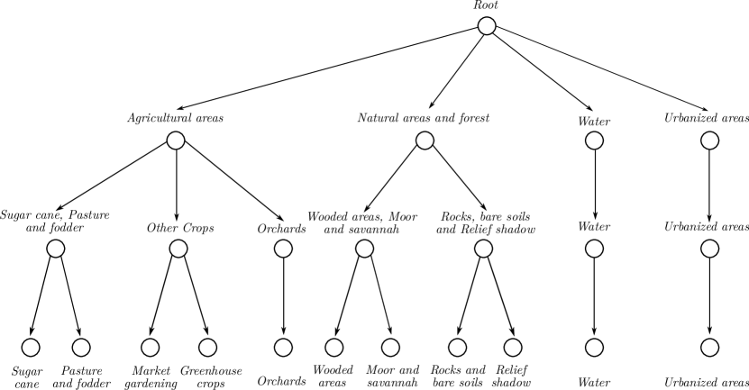
Figure 1: Representation of the Reunion island hierarchical organization

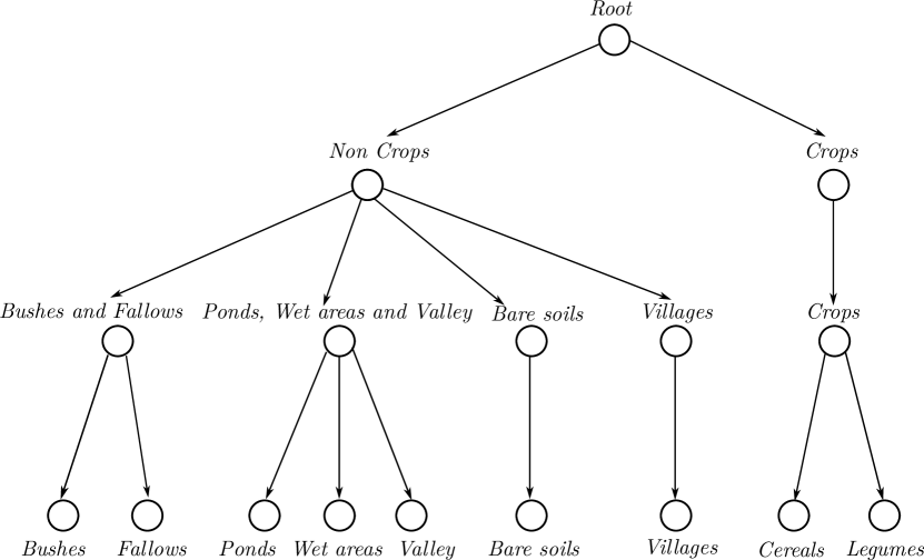
Figure 2: Representation of the Senegalese site hierarchical organization

To analyse data at object-level, a segmentation was performed for each study site using the VHSR images at hand (i.e. SPOT6/7 and PlanetScope) which have been coregistered with the corresponding Sentinel-2 grid to ensure a precise spatial matching. The VHSR images were segmented using the Large Scale Generic Region Merging (LSGRM) Orfeo Toolbox remote module [31] obtaining 14 465 (resp. 116 937) segments for the Reunion island (resp. the Senegalese site). Segmentation parameters were ajusted so that the obtained segments fit as closely as possible field plot boundaries. Then, for each study site, the ground truth data were spatially intersected with the obtained segments to provide radiometrically homogeneous class samples and it finally resulted in new comparable size labeled 7 908 segments for the Reunion island (resp. 3 084 segments for the Senegalese site). See Tables 1 and 2 for details. Finally, the mean value of the pixels corresponding to each segment was calculated over all the timestamps in the SITS, resulting in 157 variables per segment ($26\times 2$ for S1 $+$ $21\times 5$ for S2) for Reunion and 127 variables per segment ($19\times 5$ for S2 $+$ $16\times 2$ for S1) for the Senegalese groundnut basin.

3 Method

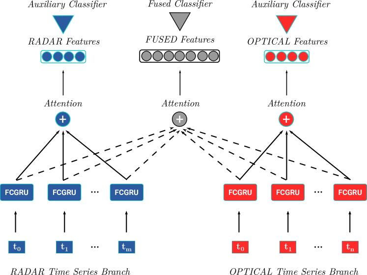
Figure 3: HOb2sRNN takes as input two time series (radar and optical SITS) and provides as output the land cover classification. The architecture is composed of two branches. Each branch firstly processes the SITS by means of a modified Gated Recurrent Unit cell we named FCGRU and, successively, a modified attention mechanism is employed on top of the FCGRU outputs to extract the per source features. Furthermore, the same attention mechanism is employed on the concatenation of the per source outputs allowing to extract fused features. Finally, the set of features (per-source and fused) extracted is leveraged to provide the final classification.

Figure 3 depicts the proposed deep learning architecture, named HOb2sRNN, for the multi-source SITS classification process. The architecture involves two branches: one for the radar (left) and one for the optical (right) time series. The output of the model is a land cover classification for each pair time series (radar and optical). Each branch of the HOb2sRNN architecture can be approximately decomposed in two parts: i) the time series analysis through the modified Gated Recurrent Unit cell we named FCGRU and ii) the multi-temporal combination to generate per-source features employing a modified attention mechanism. Moreover, the per branch FCGRU outputs are concatenated and the same attention mechanism is employed to extract fused features. Finally, the extracted per branch and fused features are leveraged to produce the final land cover classification. Such learned features named $feat_{rad}$, $feat_{opt}$ and $feat_{fused}$ indicate respectively the output of the radar branch, the optical branch and the two sources combination process. The architecture is trained leveraging specific knowledge derived from the hierarchical organization of the land cover classes.

3.1 Fully Connected Gated Recurrent Unit (FCGRU)

The first part of each branch is constituted by a modified structure of Gated Recurrent Unit (GRU) cell we named Fully Connected GRU (FCGRU). GRU [32] is a kind of Recurrent Neural Network (RNN) like Long Term Short Memory (LSTM) [33], which has demonstrated its effectiveness in the field of remote sensing [34, 35] among others. Unlike standard feed forward networks (i.e. CNNs), RNNs explicitly manage temporal (sequential) data dependencies since the output of the neuron at time $t-1$ is used, together with the next input, to feed the neuron itself at time $t$. Furthermore, this approach explicitly models the temporal correlation presents in the object time series and is able to focus its analysis on the useful portion of the time series (i.e., discarding less useful information).

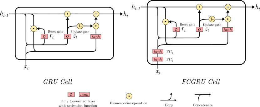
Figure 4: Visual representation of the GRU and FCGRU cells

In Figure 4 we compare the standard GRU unit with the introduced FCGRU. The main difference

is related to the fact that the latter involves two fully connected layers ($FC_{1}$ and $FC_{2}$) to preprocess the time series information before start the standard transformation involved in the GRU unit. This layer takes as input one sequence (i.e. time stamp) of the object time series (radar or optical) and combine the input data. Such layers allow the architecture to extract an useful input combination for the classification task enriching the original data representation. A Hyperbolic Tangent non-linearity function ($tanh$) is associated to each of the fully connected layers. Successively, the standard GRU unit is employed. It is composed

of a hidden state $h_{t}-1$, and two different gates: the reset gate $r_{t}$ and the update gate $z_{t}$. The gates have two important functions: i) they regulate how much information has to be forgotten/remembered during the process and ii) they deal with the vanishing/exploding gradient problem. The gates are implemented by a Sigmoid function ($\sigma$) returning values between 0 and 1. The output of the unit is the new hidden state $h_{t}$. The following equations formally describe the FCGRU cell:

$$x_{t^{\prime}}=\tanh(W_{2}\tanh(W_{1}x_{t}+b_{1})+b_{2})$$ (1)

$$z_{t}=\sigma(W_{zx}x_{t^{\prime}}+W_{zh}h_{t-1}+b_{z})$$ (2)

$$r_{t}=\sigma(W_{rx}x_{t^{\prime}}+W_{rh}h_{t-1}+b_{r})$$ (3)

$$h_{t}=z_{t}\odot h_{t-1}+(1-z_{t})\odot\tanh(W_{hx}x_{t}+W_{hr}(r_{t}\odot h_{t-1})+b_{h})$$ (4)

The $\odot$ symbol indicates an element-wise multiplication while $\sigma$ and $\tanh$ represent Sigmoid and Hyperbolic Tangent function, respectively. $x_{t}$ is the time stamp input vector and $x_{t^{\prime}}$ is the enriched input vector representation. The different $W_{*}$, $W_{**}$ matrices and bias coefficients $b_{*}$ are the parameters learned during the training of the model. Dropout was employed in the FCGRU cell and between the two fully connected layers to prevent overfitting.

3.2 Modified Attention Mechanism

The second part of the branches consists of a modified neural attention mechanism on top of the output hidden states produced by the FCGRU layer. Attention strategies [36, 37, 38] are widely used in automatic signal processing (1D signal or language) as they allow to join together the information extracted by the RNN model at different time stamps via a convex combination of the input sources. Attention was initially designed in the context of Neural Machine Translation using sequence to sequence (seq2seq) models [39], to deal with long sequences sentences which decrease such models performances. The traditional seq2seq models are composed of a RNN encoder and decoder. A context (thought) vector summarizing (encoding) the encoder states is then used by the decoder to predict the output sequences, discarding the encoder intermediate states. In attention models, instead of throwing away those intermediate states, the model uses them to construct the context vector required by the decoder. The hypothesis is that all the states are not necessary relevant when trying to predict a specific target sequence (word). Therefore, a score (attention weight) is computed for each intermediate state as the decoder will ”pay more attention” to states which get high weights in the target sequence predicting. The attention weights are commonly computed using a $SoftMax$ function so that their values range is [0,1] and their sum is equal to 1 providing at the same time a probabilistic interpretation. Finally, the context vector is computed by weighted each intermediate state with the attributed weight.

However, in the remote sensing time series classification context, where no decoder is required, using a $SoftMax$ function forcing the sum of weights to 1 may not be fully beneficial for the attention model. In fact, considering a specific time-series classification task where almost all the time stamps are relevant for the problem, the use of a SoftMax function to compute attention weights will squash towards zero the attention weights since their sum should be one and finally the attention combination may not be efficient as expected. Relaxing this constraint could thus help to better weight the relevant time stamps independently. Therefore, in our attention formulation, we attempt to address this point by substituting the $SoftMax$ function with a Hyperbolic Tangent function in the attention weight computation. The motivation behind the $tanh$ neural attention apart from relaxing the sum constraint is that the learned weights will be in a wider range i.e. [-1,1], also allowing negative scores to be mapped as negative weights. The equations below describe the $tanh$ attention formulation we introduce:

$$score=tanh(H\cdot W+b)\cdot u$$ (5)

$$\lambda=tanh(score)$$ (6)

$$feat=\sum_{i=1}^{N}\lambda_{i}h_{t_{i}}$$ (7)

where $H\in\mathbb{R}^{N,d}$ is a matrix obtained by vertically stacking all hidden state vectors $h_{t_{i}}\in\mathbb{R}^{d}$ learned at $N$ different timestamps by the FCGRU; $\lambda\in\mathbb{R}^{d}$ is the attention weight vector traditionally computed by a $SoftMax$ function which we replaced by a $tanh$ function; matrix $W\in\mathbb{R}^{d,d}$ and vectors $b,u\in\mathbb{R}^{d}$ are parameters learned during the process.

The described attention mechanism is employed over the FCGRU outputs (hidden states) in the radar and optical branches to generate per-source features ($feat_{rad}$ and $feat_{opt}$). Such features encode the temporal information related to the input source. Furthermore, the per-source hidden states are concatenated and an additional attention mechanism is employed over them to generate fused features ($feat_{fused}$). Such fused features encode both temporal information and complementarity of radar and optical sources. Thus, the architecture involves learning three sets of attention weights: $\lambda_{rad}$, $\lambda_{opt}$ and $\lambda_{fused}$ which refers respectively to the attention mechanisms employed over the radar hidden states, the optical hidden states and the concatenated ones.

3.3 Feature combination

Once each set of features has been yielded, they are directly leveraged to perform the final land cover classification. The combination process involves three classifiers: one classifier on top of the fused features ($feat_{fused}$) and two auxiliary classifiers, one for each source ($feat_{rad}$ and $feat_{opt}$). Auxiliary classifiers [40, 10, 14] are used to strengthen the complementarity as well as the discriminative power of the per-source learned features. The goal of this extra classifiers is to stress the fact that the learned features need to be discriminative alone i.e. independently from each other.

Then, the cost function associated to the optimization of the three classifiers is:

$$\footnotesize L_{total}=0.5*L(feat_{rad})+0.5*L(feat_{opt})+L(feat{fused})$$ (8)

where $L(feat)$ is the loss function (in our case the categorical Cross-Entropy) associated to the classifier fed with the features $feat$.

The contribution of each auxiliary classifier was empirically weighted by 0.5 to enforce the discriminative power of the per-source learned features while privileging the fused features in the combination. The final land cover class is derived combining the three classifiers with the same weight schema employed in the loss function computation:

$$score=0.5\times score_{rad}+0.5\times score_{opt}+score_{fused}$$ (9)

where $score_{fused}$, $score_{rad}$ and $score_{opt}$ are the predictions of the fused classifier, the classifier considering the radar SITS and that considering the optical SITS, respectively.

3.4 Hierarchical pretraining strategy

Considering real-world scenario, when field campaigns are performed, information on a plot can be collected considering multiple level of details. For instance, given a plot, the expert collects the ground truth, filling firstly the vegetation land cover, then the crop type and finally the crop.

Therefore, considering the simplest to the most complex level, we can derive a hierarchical organization about land cover classes, as illustrated in Figure 5, which could be fruitful to consider in the land cover classification process.

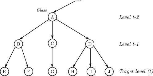
Figure 5: Representation of a land cover class hierarchical organization

With the aim to leverage such a precious knowledge, the HOb2sRNN architecture was trained in a hierarchical manner exploiting such taxonomic organization of the land cover classes. The training is repeated for each level of the hierarchy, from the more general one (the most simple) to the most specific one (the target classification level).

Specifically, we start the model training on the  highest level of the hierarchy and subsequently, we continue the training on the next level reusing the previous learned weights for the whole architecture, excepting the weights associated to the output layer since level-specific. This process is performed until we reach the target level. New classifiers (output layers) were trained for each level of the hierarchy. To sum up, such hierarchical pretraining strategy allows the model to focus firstly on easy classification problems (i.e. Crops vs Non Crops) and, step by step, the network behavior is adapted smoothly to deal with classification problems with increasing complexity levels. In addition, this process allows the classification model to tackle the classification at the target level (the most specific level of the land cover hierarchy) integrating a kind of prior knowledge on the task instead of addressing it completely from scratch.

4 Experimental evaluation

In this section, we present and discuss the experimental results obtained on the study sites introduced in Section 2. We carried out several experimental analysis in order to provide a deep assessment of the HOb2sRNN behaviour:

• an in-depth evaluation of the quantitative performances of the HOb2sRNN with respect to several other competitors;

• an ablation study on sources (Sentinel-1/Sentinel-2) as well as on the different components of the HOb2sRNN architecture to characterize the interplay among them;

• a qualitative analysis of land cover maps considering the HOb2sRNN and its competitors;

• an inspection of the attention parameters learnt by our architecture, in order to investigate to what extent such side information can contribute to the model interpretability.

4.1 Experimental settings

To assess the quality of HOb2sRNN, we chosen as competitors common machine learning techniques which are the de facto baselines in the field of remote sensing, commonly employed to deal with SITS data [18]: Random Forest (RF) and Support Vector Machine (SVM). In addition, we also consider a Multi Layer Perceptron neural net (MLP). The competing methods were run over the concatenation of the different information sources: Sentinel-1 and Sentinel-2 SITS. We optimize the model parameters via train/validation procedure [27]. The settings are reported in Table 3. The datasets were split into training, validation and test set with an object proportion of 50%, 20% and 30% respectively. The values were normalized per band (resp. indices) considering the time series, in the interval $[0,1]$. Training data are used to learn the model while validation data are exploited for model selection. Finally, the model achieving the best accuracy on the validation set was employed to classify the test set. We imposed that segments belonging to the same ground truth polygon before the spatial intersection (see Section 2.3) were assigned exclusively to one of the data partitions (training, validation or test) to avoid a possible spatial bias in the evaluation procedure. The assessment of the classification performances was done considering Accuracy (global precision), F1 Score and Kappa metrics. Since the model performances may vary depending on the split of the data due to simpler or more complex samples involved in the different partition, all metrics were averaged over ten random splits following the strategy previously reported. Experiments were carried out on a workstation with an Intel (R) Xeon (R) CPU E5-2667 v4@3.20Ghz with 256 GB of RAM and four TITAN X GPU. The neural architectures were implemented using the Python Tensorflow library, while machine learning algorithms implementation were obtained from the Python Scikit-learn library [41].

Table 3: Hyper-parameters and corresponding value or ranges of all the competing methods

Method	Hyper-Parameter	Value or Range
HOb2sRNN	Epoch number	2000 per level
	FCGRU units	512
	FC1 units	64
	FC2 units	128
MLP	Epoch number	2000
	Hidden units	512
	Hidden layers	2
HOb2sRNN	Batch size	32
	Dropout rate	0.4
and MLP	Optimizer	Adam [42]
	Learning rate	$1\text{\times}{10}^{-4}$
RF	Tree number	{100, 200, 300,400,500}
	Maximum depth	{20,40,60,80,100}
	Maximum features	{’sqrt’, ’log2’, None}
SVM	Kernel	{’linear’, ’poly’, ’rbf’, ’sigmoid’}
	Gamma	{0.25,0.5,1,2}
	Penalty	{0.1, 1, 10}

4.2 Comparative analysis

In this part, we compare the results obtained by the different competing methods, considering their overall and per-class scores.

4.2.1 General behavior

Table 4 reports the averaged results obtained for RF, SVM, MLP and HOb2sRNN on the Reunion island and the Senegalese groundnut basin site. Considering the averaged performances, we can state that the proposed method outperforms its competitors on both study sites. However, the performance gaps are better pronounced on the Reunion island dataset than the Senegalese site one. This behavior may be due to the fact that the Reunion island dataset represents a more rich benchmark (about 8 times) than the Senegalese dataset in terms of ground truth samples. In fact, it is known that deep learning models get more and more accurate when learning from huge volumes of data. Concerning the other competing methods i.e. RF and SVM, they achieve similar scores on the Reunion island while SVM surpasses RF on the Senegalese site. On this latter benchmark, the SVM algorithm demonstrates to be well suited for dataset characterized by a limited set of labeled samples. As regards the MLP competitor, it achieves lower scores than HOb2sRNN on the Reunion island while scores are comparable on the Senegalese site. It should be noted that the relatively better performance obtained on the Senegalese site compared to the Reunion island (90.78 vs. 79.66) may come from the topography of the study sites. In fact, Reunion island is characterized by a rugged topography while the Senegalese site is essentially flat. Relief effects like shadow or orientation can induce biases in the discrimination of land cover classes impacting much more the Reunion island [14].

Table 4: F1 score, Kappa and Accuracy considering the different methods (RF, SVM, MLP and HOb2sRNN) on each study site (results averaged over ten random splits)

Site	Method	F1 score	Kappa	Accuracy
Reunion	RF	75.62 $\pm$ 1.00	0.726 $\pm$ 0.011	75.75 $\pm$ 0.98
	SVM	75.34 $\pm$ 0.88	0.722 $\pm$ 0.010	75.39 $\pm$ 0.89
	MLP	77.96 $\pm$ 0.70	0.752 $\pm$ 0.008	78.03 $\pm$ 0.66
	HOb2sRNN	79.66 $\pm$ 0.85	0.772 $\pm$ 0.009	79.78 $\pm$ 0.82
Senegal	RF	86.31 $\pm$ 0.91	0.828 $\pm$ 0.012	86.35 $\pm$ 0.90
	SVM	89.95 $\pm$ 0.85	0.875 $\pm$ 0.011	89.96 $\pm$ 0.85
	MLP	90.05 $\pm$ 0.56	0.876 $\pm$ 0.007	90.07 $\pm$ 0.57
	HOb2sRNN	90.78 $\pm$ 1.03	0.885 $\pm$ 0.013	90.78 $\pm$ 1.03

4.2.2 Per-class analysis

Tables 5 and 6 report the per-class F1 scores obtained by the different methods on the Reunion island and the Senegalese site, respectively. Concerning the Reunion site, we can observe that HOb2sRNN achieves the best performances on the majority of land cover classes excepted some classes where other competing methods i.e. RF or MLP obtained slightly better scores that are still comparable to the ones achieved by our framework. It is worth noting how the proposed method outperforms its competitors particularly on agricultural/vegetation classes i.e. classes $0$–Sugar cane, $1$–Pasture and fodder, $2$–Market gardening, $3$–blackhouse crops and $4$–Orchards. The best gain (5 points from the best competitor) is obtained on $1$–Pasture and fodder class. This particular efficiency on such classes suggest that the HOb2sRNN architecture is well suited to deal with the temporal dependencies characterizing these land cover classes. As regards the Senegalese site, the per-class HOb2sRNN performances are more moderate. It achieves the best scores on 4 land cover classes over 9 i.e. $1$–Fallows, $2$–Ponds, $7$–Cereals and $8$–Legumes while other competing methods outperformed its results especially on the $6$–Valley class. Nonetheless, it should be remarked that also in this case, HOb2sRNN obtained the best results on land cover classes which exhibit a time-varying behavior. It is common to observe natural vegetation activity on fallows areas; ponds appear during the rainy season while cereals and legumes follow crop growth cycle. These findings are inline with the previous observations made on the Reunion island and confirm the fact that the proposed method is capable to fruitfully leverage temporal dependencies to made its decision.

Table 5: Per-Class F1 score for the Reunion island (average over ten random splits)

Method	$0$–Sugar cane	$1$–Pasture and fodder	$2$–Market gardening	$3$–blackhouse crops	$4$–Orchards	$5$–Wooded areas	$6$–Moor and Savannah	$7$–Rocks and bare soil	$8$–Relief shadows	$9$–Water	$10$–Urbanized areas
RF	83.34	76.13	66.39	47.85	67.16	83.10	75.09	81.81	93.51	78.44	74.54
SVM	83.61	74.46	64.12	50.69	68.40	82.41	75.28	79.76	87.44	75.88	77.31
MLP	85.95	76.92	69.25	52.87	70.72	82.36	78.16	82.57	90.00	84.91	79.24
HOb2sRNN	88.67	81.26	71.73	53.43	72.19	82.62	77.44	85.71	90.61	88.77	79.05

Table 6: Per-Class F1 score for the Senegalese site (average over ten random splits)

Method	$0$–Bushes	$1$–Fallows	$2$–Ponds	$3$–Bare soils	$4$–Villages	$5$–Wet areas	$6$–Valley	$7$–Cereals	$8$–Legumes
RF	73.10	81.03	78.34	92.54	97.86	83.67	92.29	81.49	82.99
SVM	82.08	82.95	87.08	93.84	99.04	91.12	92.04	86.64	87.09
MLP	82.37	84.04	84.96	93.90	98.98	90.51	90.27	86.97	87.15
HOb2sRNN	80.68	86.20	89.12	91.84	98.78	89.84	88.52	87.71	89.34

To go further with the per-class analysis, we also investigate the confusions matrices of each method on the two study sites. Concerning the Reunion island (Figure 6), all the methods exhibit similar behaviors. This is particularly evident between $3$–blackhouse crops and $10$–Urbanized areas class even if confusion are reduced from RF (Figure 6a) to HOb2sRNN as can be observed (Figure 6d). Overall, the per-class analysis is coherent with the findings we got in the previous analysis. Apropos of the Senegalese site (Figure 7), confusions vary sensibly regarding the different methods. RF (Figure 7a) exhibits more confusions on $0$–Bushes and $1$–Fallows classes which are highly misclassified with $7$–Cereals class and a little bit less with $8$–Legumes class while $2$–Ponds are often confused with $5$–Wet areas. The other competitors tend to reduce these confusions as also evidenced by the confusion matrix colours.

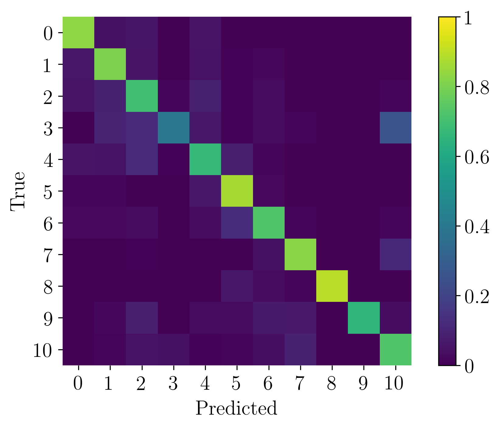
(a) RF

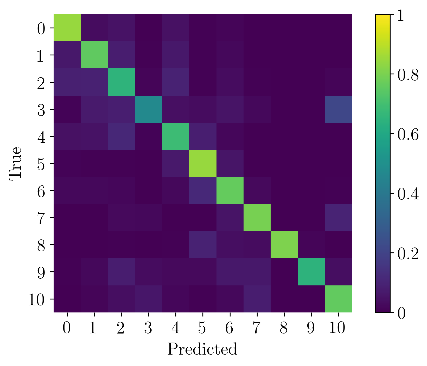
(b) SVM

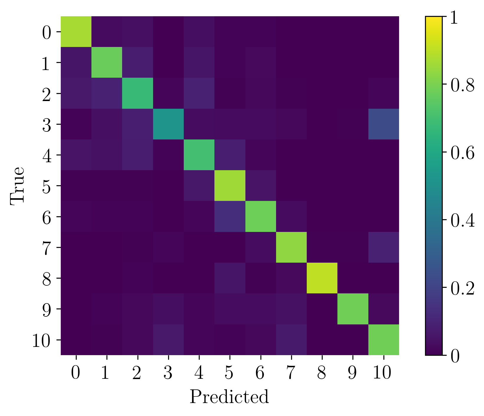
(c) MLP

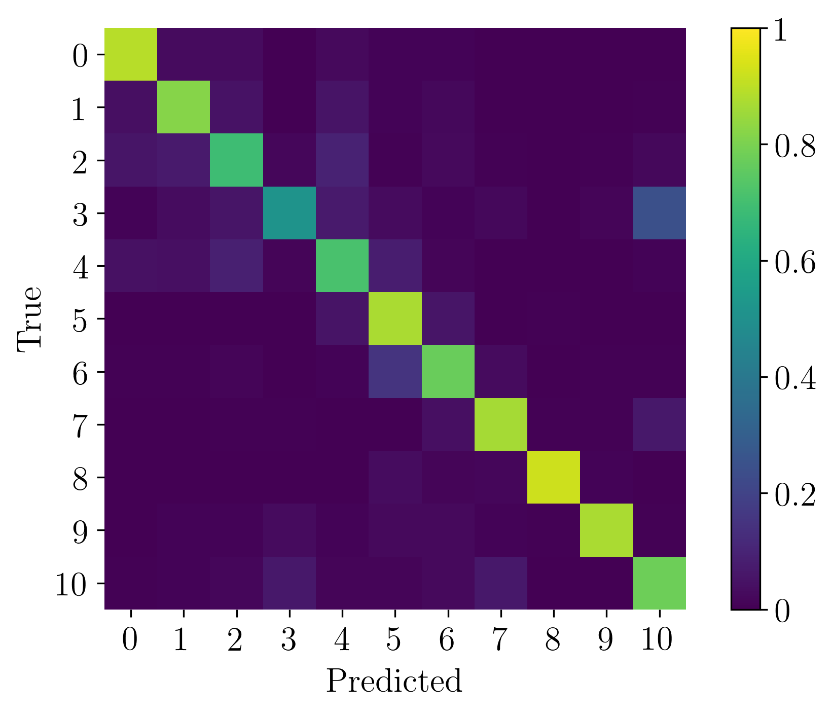
(d) HOb2sRNN

Figure 6: Confusion Matrices of the land cover classification produced by (a) RF, (b) SVM, (c) MLP and (d) HOb2sRNN on the Reunion island.

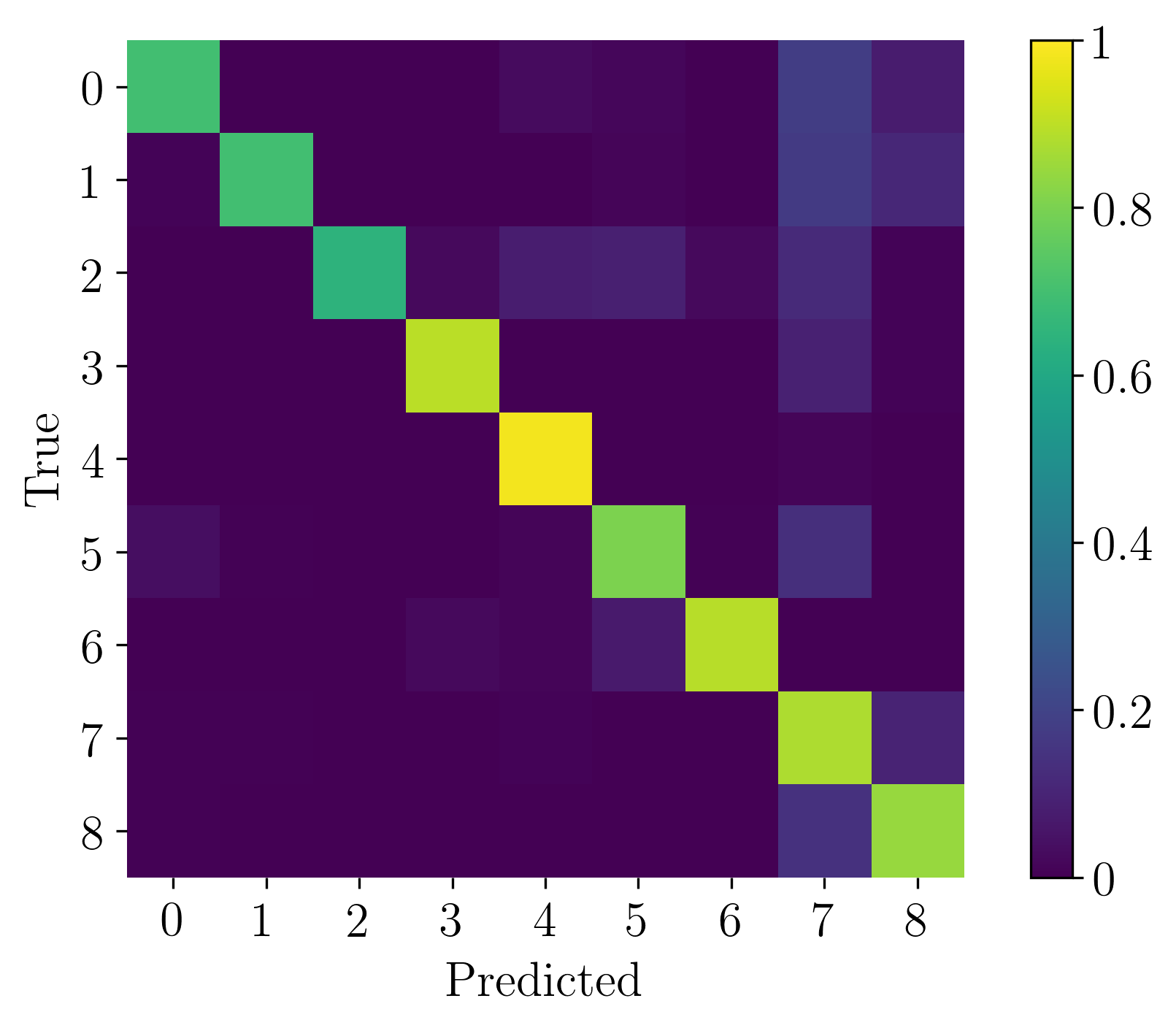
(a) RF

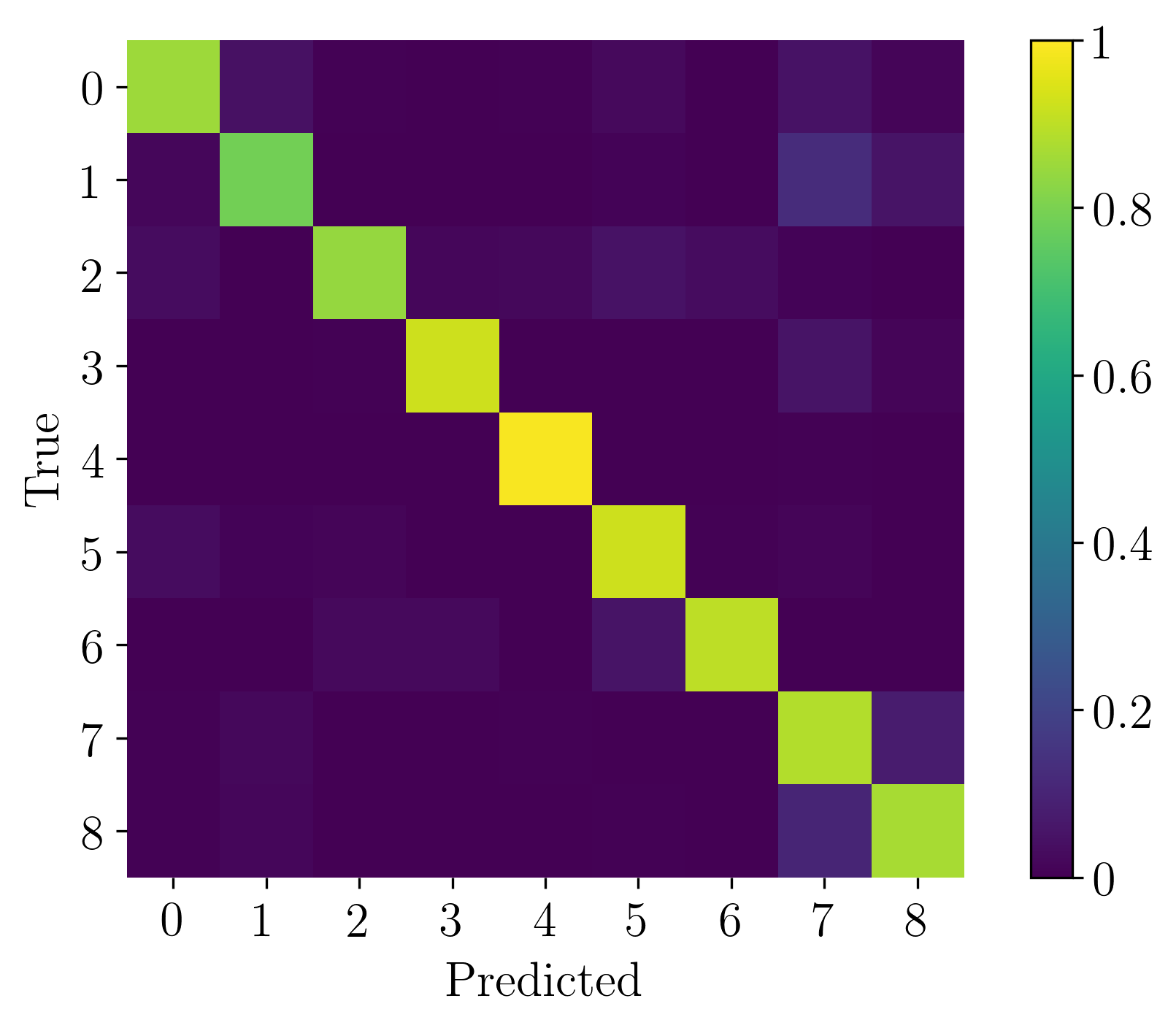
(b) SVM

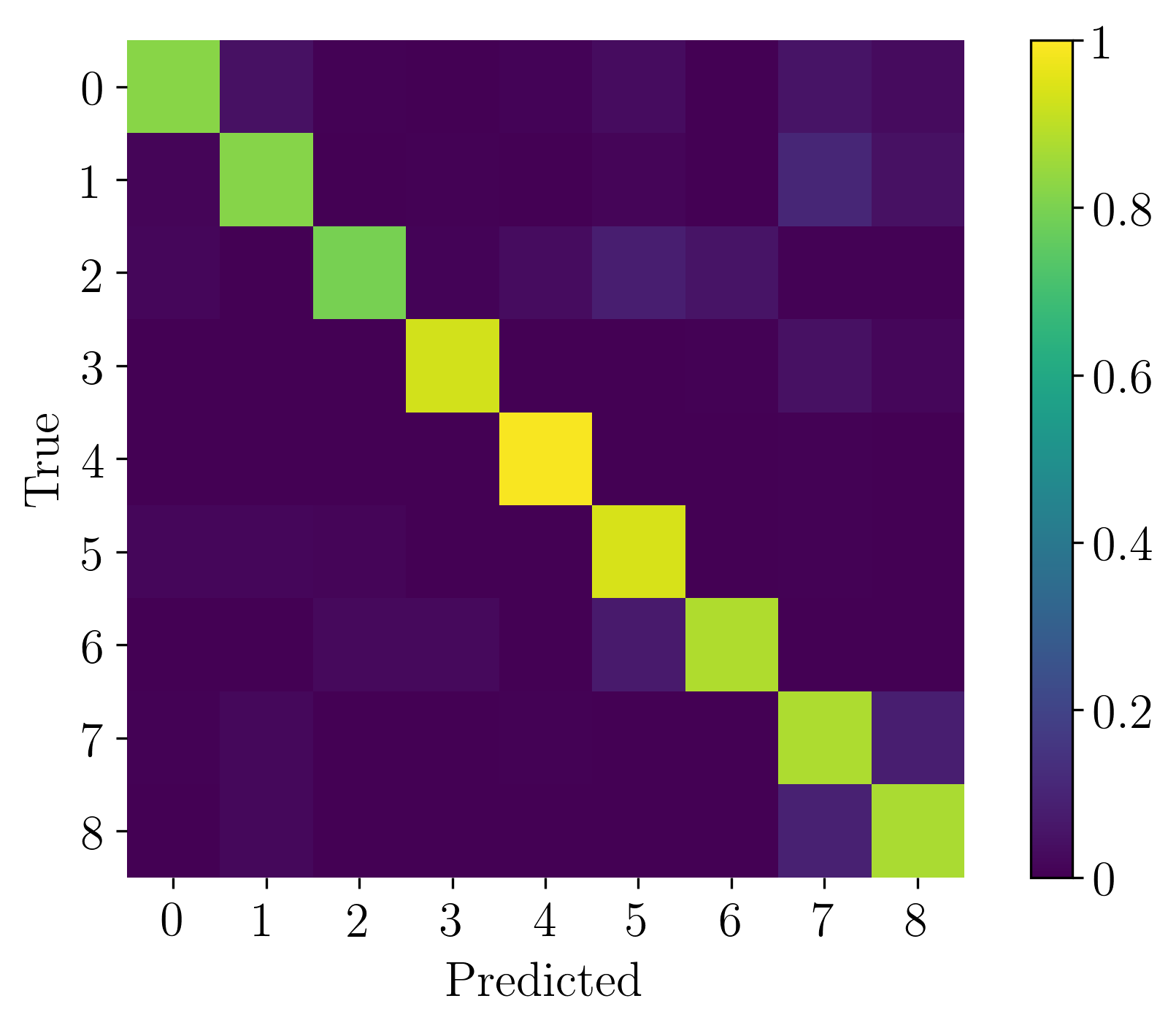
(c) MLP

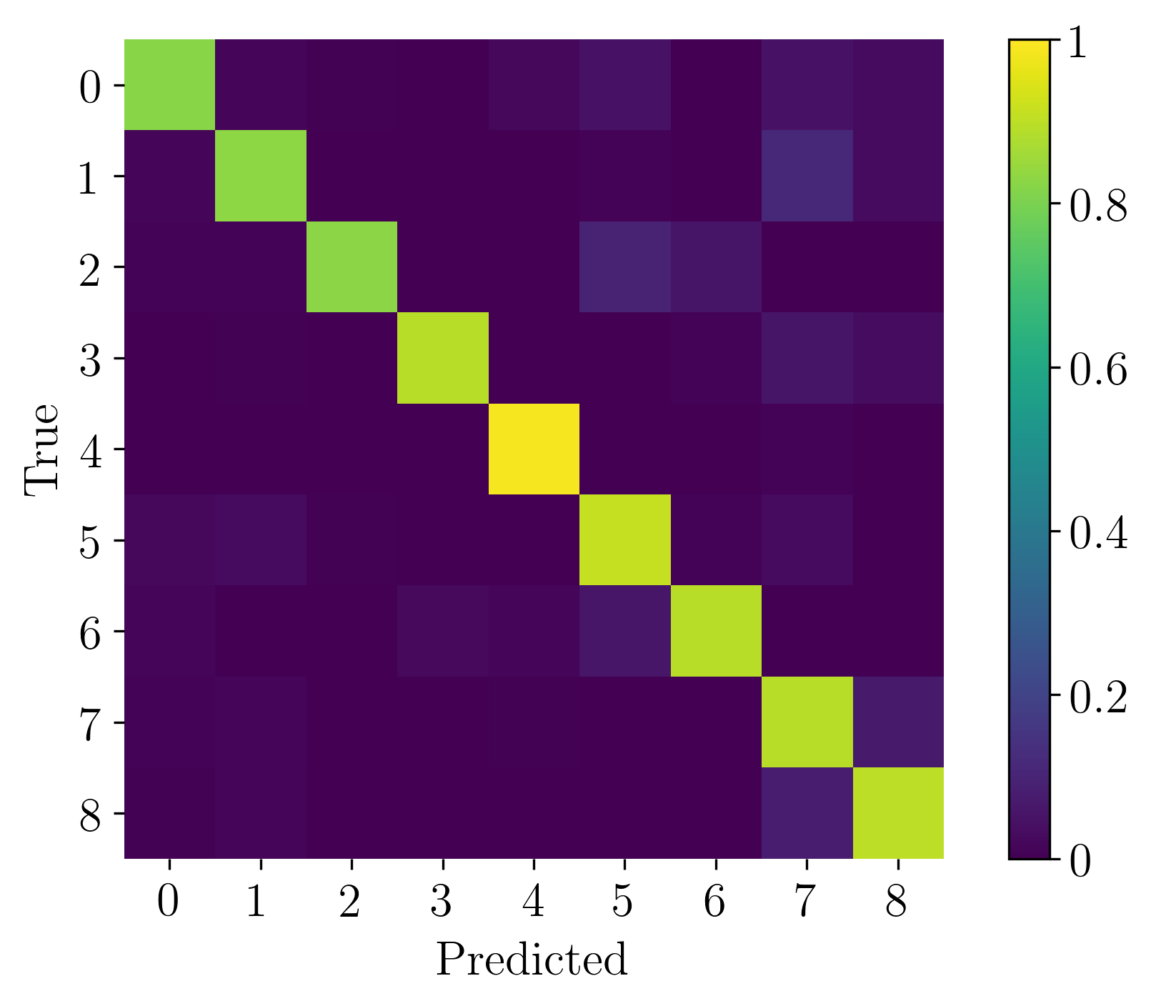
(d) HOb2sRNN

Figure 7: Confusion Matrices of the land cover classification produced by (a) RF, (b) SVM, (c) MLP and (d) HOb2sRNN on the Senegalese site.

4.3 Ablation analysis

Here, we conduct several stages of ablation experiments considering the multi-source SITS and the architecture components. In addition, we provide an assessment of the NDVI index helpfulness, used as extra optical descriptor, for the HOb2sRNN architecture.

4.3.1 Ablation on multi-source SITS

In this stage of experiments, we consider only one source of time series (radar or optical) to perform the land cover classification. We name HOb2sRNN(S1) (resp. HOb2sRNN(S2) ) the ablation of our model considering the radar (resp. optical) branch. To better figure out how each source of SITS is leveraged, we also report the competing method performances (RF, SVM and MLP) in this per-source ablation analysis. Their variants are named in the same manner.

Regarding the results reported in Table 7, the radar time series has a specific behavior for each of the considered study sites. If radar signal is quite discriminating in the Senegalese site, this is not really the case for the Reunion island considering how poorly the competing methods trained on the radar SITS perform, especially the SVM algorithm. Thus on the Reunion island, non temporal based models i.e. (RF, SVM and MLP) perform slightly worst or equally on the concatenation of 2 sources than learning only with optical data. However, HOb2sRNN performs better when combining the two time series sources. This behavior suggests that HOb2sRNN is able to better leverage the complementarity between radar and optical data than its competitors. This behavior is also evident in the Senegalese site where all competing methods perform better with both sources but HOb2sRNN is the one that performs the best. For the rest, considering the two study sites, there is no trend on which competing methods better deal with radar or optical time series than others. However, we have observed on both sites that SVM algorithm seems not well suited to exploit radar information.

Table 7: F1 score, Kappa and Accuracy of the different methods (RF, SVM, MLP and HOb2sRNN) considering the per-source ablation analysis on the study sites (results averaged over ten random splits). Refer to Table 4 for the results of SITS combination.

Site	Classifier	F1 score	Kappa	Accuracy
Reunion	RF(S1)	36.77 $\pm$ 0.93	0.291 $\pm$ 0.011	37.85 $\pm$ 0.95
	SVM(S1)	6.56 $\pm$ 0.36	0.018 $\pm$ 0.009	16.85 $\pm$ 0.53
	MLP(S1)	34.93 $\pm$ 1.42	0.271 $\pm$ 0.016	36.01 $\pm$ 1.39
	HOb2sRNN(S1)	31.80 $\pm$ 1.10	0.231 $\pm$ 0.011	32.39 $\pm$ 1.04
	RF(S2)	76.24 $\pm$ 0.59	0.732 $\pm$ 0.007	76.32 $\pm$ 0.63
	SVM(S2)	75.55 $\pm$ 0.80	0.724 $\pm$ 0.009	75.60 $\pm$ 0.80
	MLP(S2)	77.95 $\pm$ 0.69	0.751 $\pm$ 0.008	77.98 $\pm$ 0.73
	HOb2sRNN(S2)	78.69 $\pm$ 0.95	0.761 $\pm$ 0.010	78.79 $\pm$ 0.91
Senegal	RF(S1)	75.71 $\pm$ 1.03	0.703 $\pm$ 0.013	76.56 $\pm$ 1.00
	SVM(S1)	71.27 $\pm$ 0.82	0.653 $\pm$ 0.010	72.82 $\pm$ 0.78
	MLP(S1)	78.96 $\pm$ 1.28	0.738 $\pm$ 0.015	79.05 $\pm$ 1.23
	HOb2sRNN(S1)	77.42 $\pm$ 1.33	0.721 $\pm$ 0.016	77.63 $\pm$ 1.27
	RF(S2)	84.51 $\pm$ 1.17	0.806 $\pm$ 0.015	84.60 $\pm$ 1.17
	SVM(S2)	88.64 $\pm$ 0.47	0.858 $\pm$ 0.006	88.63 $\pm$ 0.45
	MLP(S2)	88.38 $\pm$ 0.61	0.855 $\pm$ 0.008	88.40 $\pm$ 0.62
	HOb2sRNN(S2)	87.56 $\pm$ 1.33	0.845 $\pm$ 0.017	87.55 $\pm$ 1.33

4.3.2 Ablation on architecture components

In this part, we investigate the interplay among the different components of HOb2sRNN and we disentangle their benefits in the architecture. We consider both time series (radar and optical) but excluding one of the following components at a time: the three attention mechanisms involved in the architecture (naming $NoAtt$), the hierarchical pretraining process (naming $NoHierPre$) and the enrichment step in the FCGRU cell which is equivalent to use a GRU cell (naming $NoEnrich$). We also investigate the use of the traditional $SoftMax$ attention mechanism instead of the modified one. This variant is named $SoftMaxAtt$. Results are reported in Table 8.

Concerning the use of attention mechanisms or not ($NoAtt$, $SoftMaxAtt$ and HOb2sRNN), we can observe how these components contribute to the final classification performances on both study sites, more on the Reunion island (about 2 points of improvement) than the Senegalese site (approximately 1 point). We can also note that $SoftMax$ attention performs relatively similar than the non use of attention mechanisms and lower than the $tanh$ attentions confirming our hypothesis that relaxing the constraint that the attention weights may sum to 1 in the attention process is more suitable for remote sensing context. As regards the use of the hierarchical pretraining process ($noHierPre$ and HOb2sRNN), we can note here the added value of such step on both study sites obtaining more than 1 point of improvement. These results seem to underline that involving domain specific knowledge in the pretraining process of neural networks can improve the final classification performances. Finally, the new FCGRU cell compared to the GRU cell ($noEnrich$) performs better in both study sites, however it seems to be more efficient in the Senegalese site.

Table 8: F1 score, Kappa and Accuracy considering different ablations of HOb2sRNN on the study sites (results averaged over ten random splits)

Site	Classifier	F1 score	Kappa	Accuracy
Reunion	$noAtt$	77.66 $\pm$ 0.99	0.749 $\pm$ 0.011	77.74 $\pm$ 0.99
	$SoftMaxAtt$	77.32 $\pm$ 1.22	0.746 $\pm$ 0.013	77.47 $\pm$ 1.18
	$noHierPre$	78.35 $\pm$ 0.70	0.756 $\pm$ 0.007	78.43 $\pm$ 0.66
	$noEnrich$	79.09 $\pm$ 0.57	0.764 $\pm$ 0.006	79.10 $\pm$ 0.50
	HOb2sRNN	79.66 $\pm$ 0.85	0.772 $\pm$ 0.009	79.78 $\pm$ 0.82
Senegal	$noAtt$	89.86 $\pm$ 0.62	0.874 $\pm$ 0.008	89.89 $\pm$ 0.63
	$SoftMaxAtt$	89.91 $\pm$ 0.54	0.874 $\pm$ 0.007	89.92 $\pm$ 0.52
	$noHierPre$	89.25 $\pm$ 0.88	0.866 $\pm$ 0.011	89.24 $\pm$ 0.87
	$noEnrich$	89.12 $\pm$ 0.64	0.864 $\pm$ 0.008	89.11 $\pm$ 0.64
	HOb2sRNN	90.78 $\pm$ 1.03	0.885 $\pm$ 0.013	90.78 $\pm$ 1.03

4.3.3 Assessment of the NDVI index helpfulness

As additional experiment, we evaluate here if the NDVI index as additional optical descriptor has an impact on the final land cover mapping obtained using the HOb2sRNN architecture. Indeed, considering NDVI index as additional feature in land cover classification task was obvious when training conventional machine learning algorithms since such techniques cannot extract specialized features for a specific task at hand [43]. Nowadays, the new paradigm related to deep (or representational) learning [43] is emerging and demonstrating to be more and more effective in the field of remote sensing [44]. Neural networks have the ability to extract features optimised for a specific task (when enough data are available) avoiding the necessity to extract hand-crafted features. Thus, employing spectral indices like NDVI as additional features to deal with land cover classification could not be necessary when using neural networks. Therefore, we evaluate on the two study sites our model performances when excluding the NDVI index in the input (optical) time series. We named such variant of the model $noNDVI$. Results are reported in Table 9.

Table 9: F1 score, Kappa and Accuracy considering the exclusion of NDVI index on the study sites (results averaged over ten random splits)

Site	Classifier	F1 score	Kappa	Accuracy
Reunion	$noNDVI$	79.83 $\pm$ 0.70	0.774 $\pm$ 0.008	79.95 $\pm$ 0.68
	HOb2sRNN	79.66 $\pm$ 0.85	0.772 $\pm$ 0.009	79.78 $\pm$ 0.82
Senegal	$noNDVI$	90.46 $\pm$ 0.82	0.881 $\pm$ 0.010	90.46 $\pm$ 0.82
	HOb2sRNN	90.78 $\pm$ 1.03	0.885 $\pm$ 0.013	90.78 $\pm$ 1.03

We can note on both study sites that there is no significant difference between HOb2sRNN and $noNDVI$ performances. $noNDVI$ performs slightly better than HOb2sRNN on the Reunion island and inversely on the Senegalese site. These small variations can come from model properties such as kernel weight initialization or parameters optimization that can induce such kind of performance fluctuations.

To conclude, this experiment underlines that our model, considering the two study sites involved in the experimental evaluation, is able to overcome the use of such common hand-crafted features achieving the same performances in the land cover mapping task. Such result makes a step further on the comprehension of which hand-crafted features are convenient (or not) to be extracted during the preprocessing step as well as save time, computation and storage resources during the analysis pipeline.

4.4 Qualitative analysis of land cover maps

With the purpose to investigate some differences in the land cover maps produced by the competing methods (RF, SVM, MLP and HOb2sRNN), we highlight in Figures 8 and 9 some representative map details of the Reunion island and the Senegalese site, respectively. For each study site, we remind that land cover maps were produced by labeling each of the segments (14 465 on the Reunion island or 116 937 on the Senegalese site) obtained after the VHSR (SPOT67 or PlanetScope) image segmentation. For each map detail, we supply the corresponding VHSR image displayed in RGB colors as reference.

Concerning Reunion island (Figure 8), we focused in the first example (Figures 8b, 8c, 8d and 8e) on the Saint-Pierre mixed coastal urban and agricultural area. In this example, we can note the confusions highlighted in the per-class analysis between urbanized areas and blackhouse crops. Visually, RF better classifies urbanized areas. The second example (Figures 8g, 8h, 8i and 8j) depicts a mixed agricultural area with natural vegetation neighboring. We can note here that HOb2sRNN is the only one which detects a realistic amount of orchard cultures according to field experts. In addition, we can also observe on the right of this extract that RF wrongly detects sugar cane plantations instead of wooded areas, moor and savannah.

Regarding the Senegalese site (Figure 9), the first example (Figures 9b, 9c, 9d and 9e) depicts a wet area near the Diohine village (in the east). While SVM, MLP and HOb2sRNN tend to provide the correct representation of the wet area, RF wrongly detects villages. As pointed out in previous map details concerning Sugar cane and Orchards on the Reunion island study site, RF predictions is sometimes biased towards most represented classes in the training data i.e. Sugar cane, Orchards in the case of Reunion island and Villages here. In fact, RF is known to be sensible to class imbalance [45]. The second example focus on a rural landscape including buildings (villages) and agricultural activities. Here, RF maps much more Legumes than its competitors while the latter detect Fallows and Cereals instead.

To sum up, these visual inspections of land cover maps are consistent with the quantitative results previously obtained.

Detail 1: A mixed coastal urban and agricultural area
Detail 2: A mixed agricultural and natural vegetation area

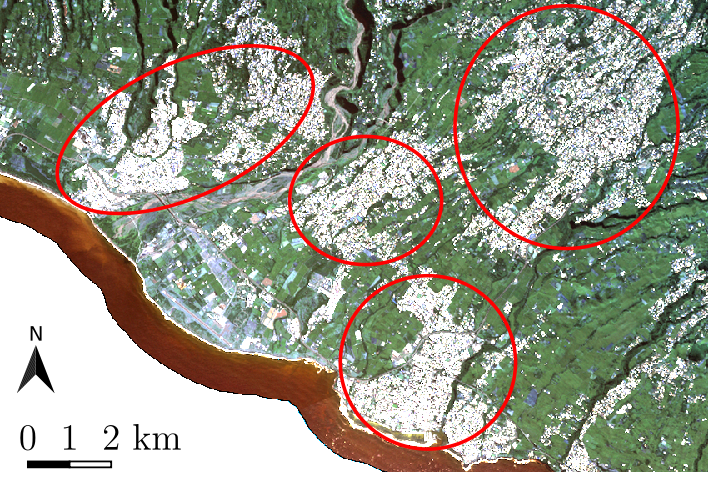
(a) RGB Image

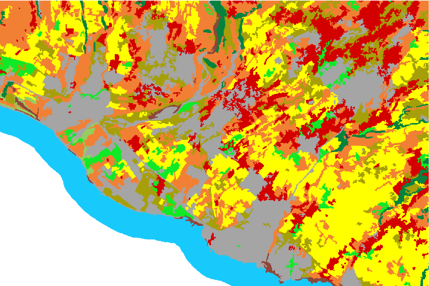
(b) RF

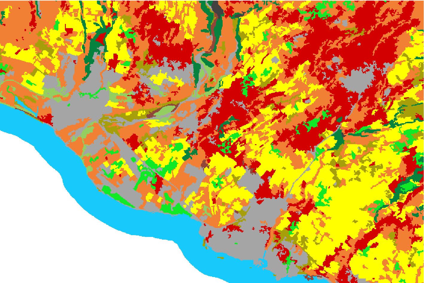
(c) SVM

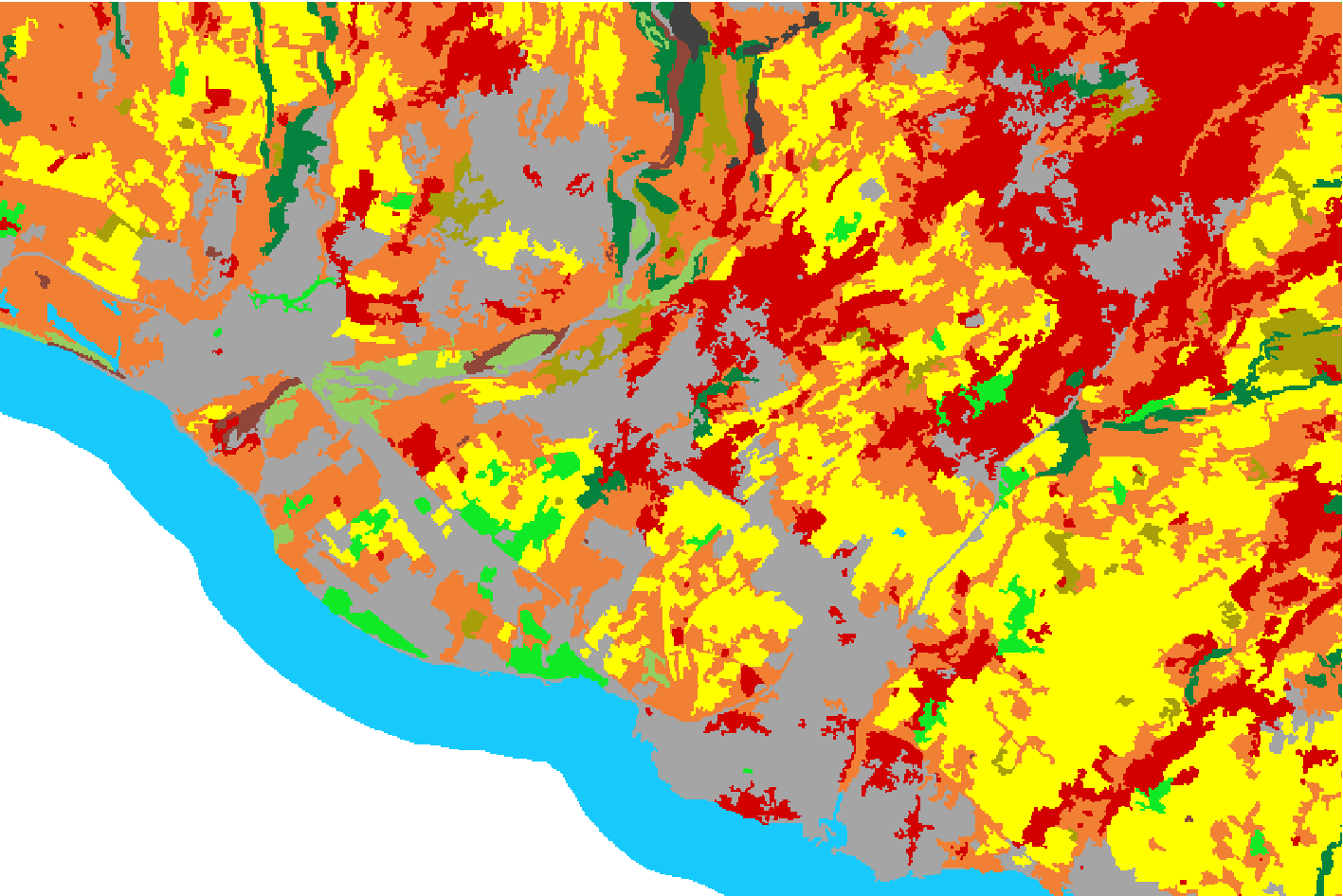
(d) MLP

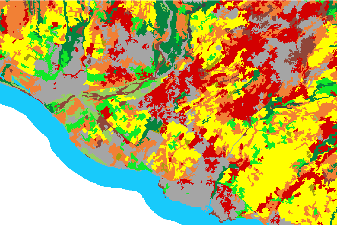
(e) HOb2sRNN

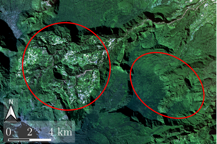
(f) RGB Image

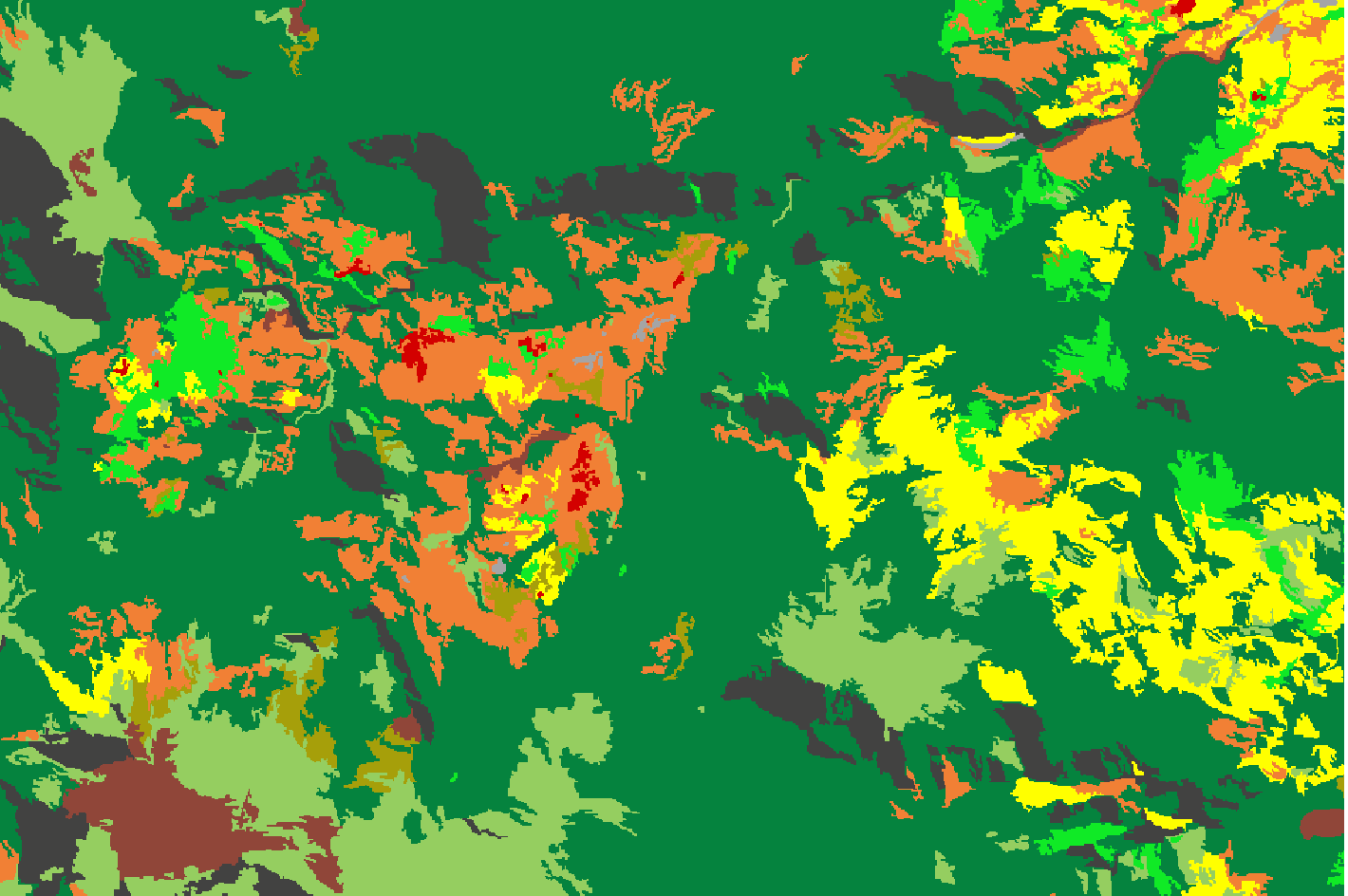
(g) RF

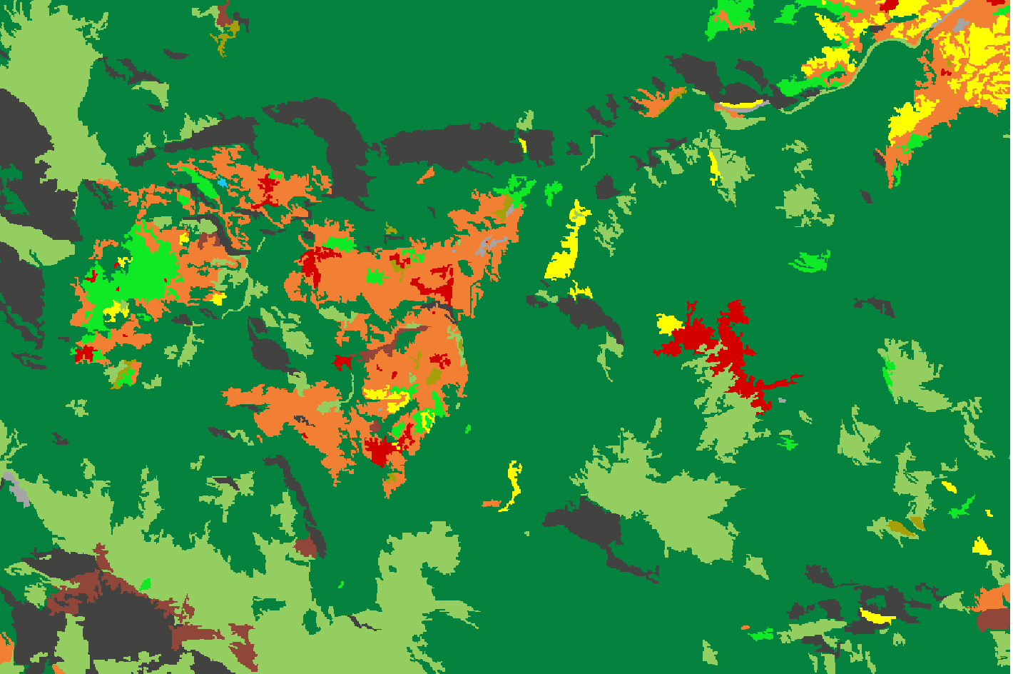
(h) SVM

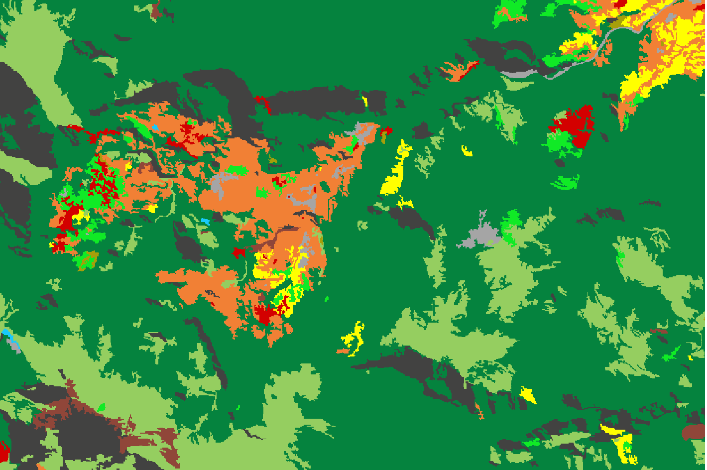
(i) MLP

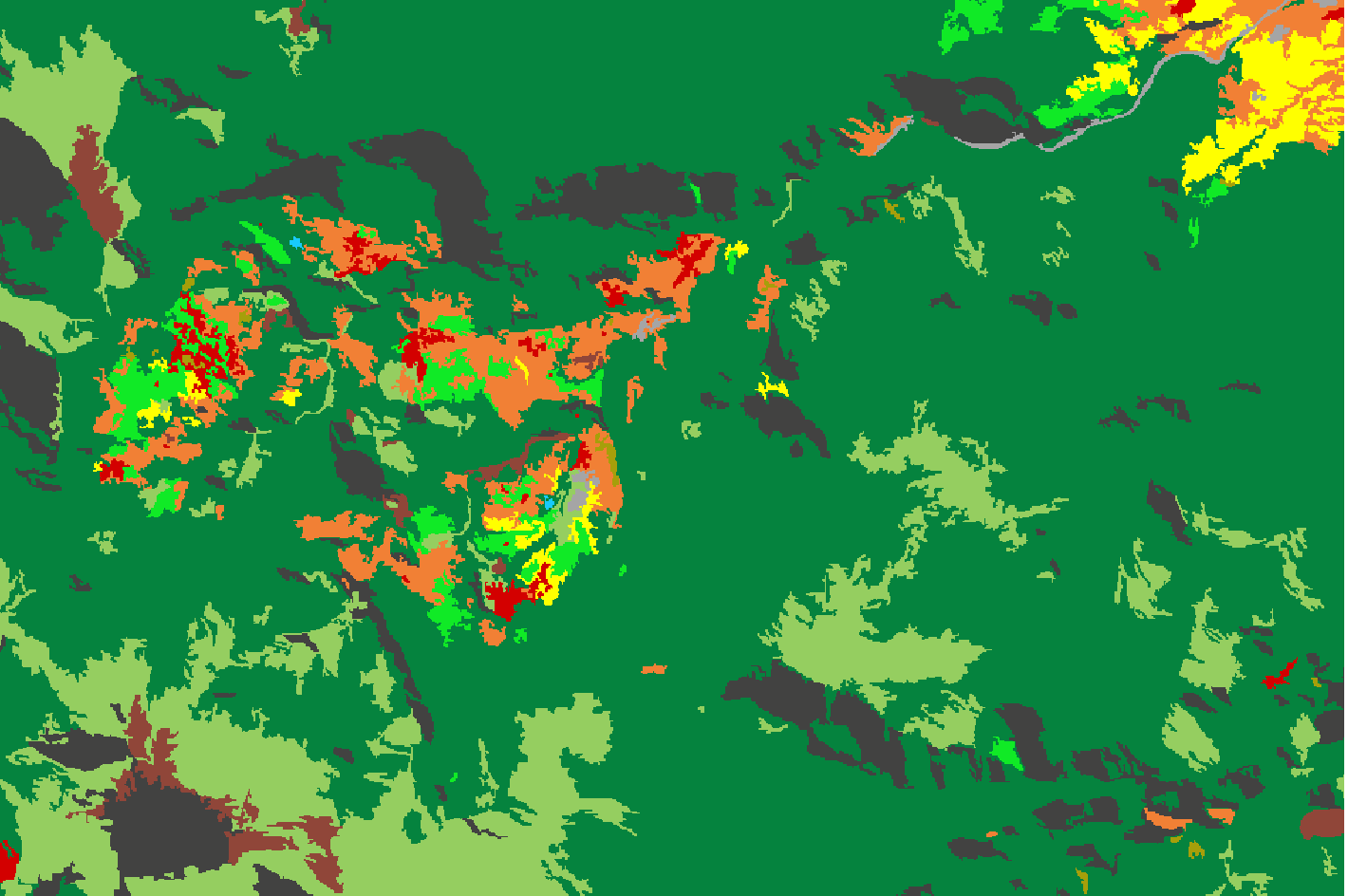
(j) HOb2sRNN

Figure 8: Qualitative investigation of land cover map details produced on the Reunion island study site by RF, SVM, MLP and HOb2sRNN on mixed urban/agricultural (top) and agricultural/natural vegetation (bottom) areas.

Detail 1: A rural landscape including a wet area
Detail 2: A rural landscape including buildings and agricultural activities

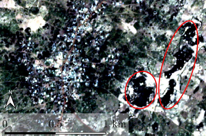
(a) RGB Image

(b) RF

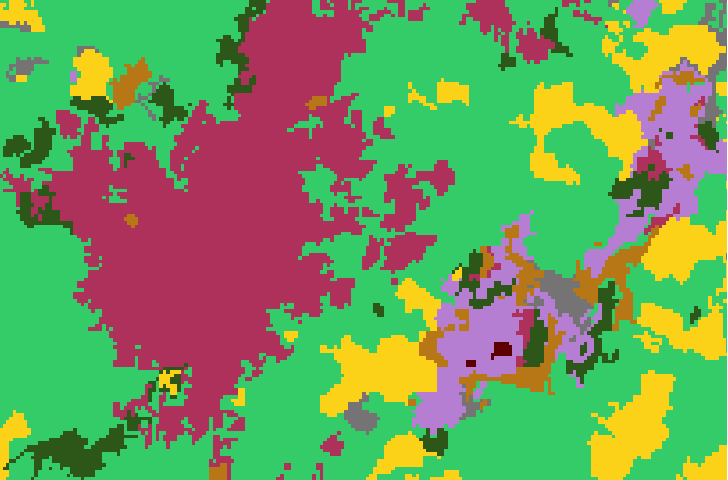
(c) SVM

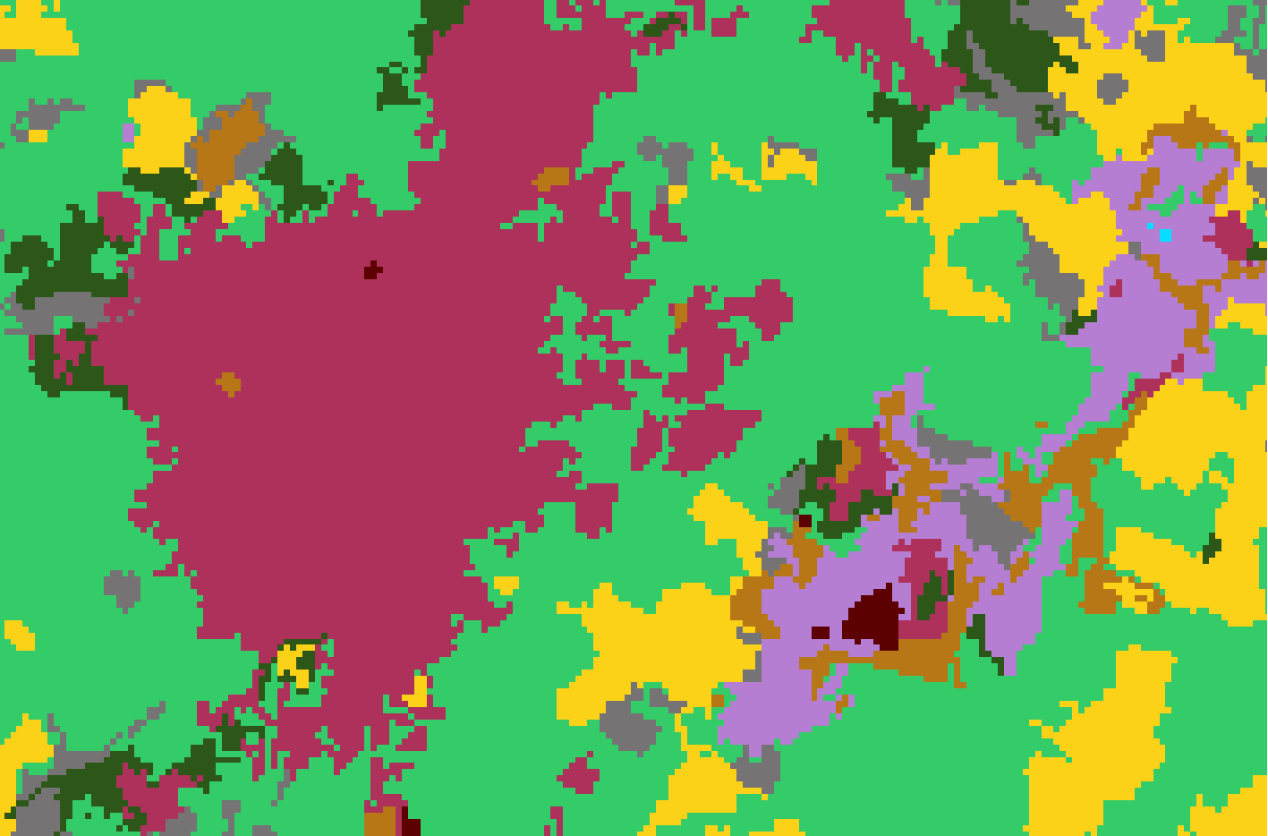
(d) MLP

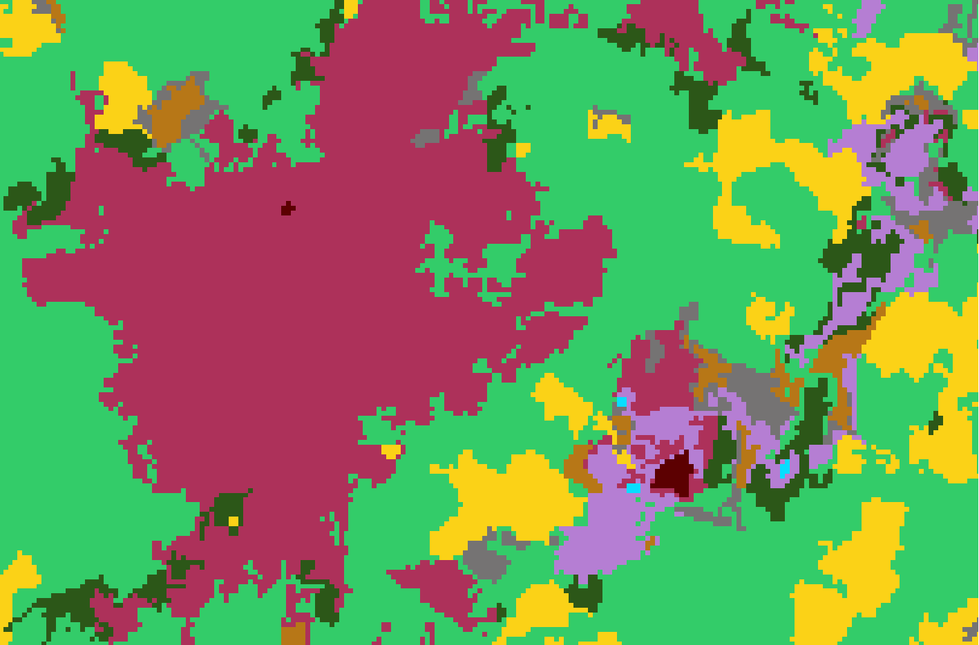
(e) HOb2sRNN

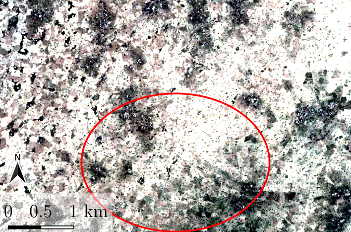
(f) RGB Image

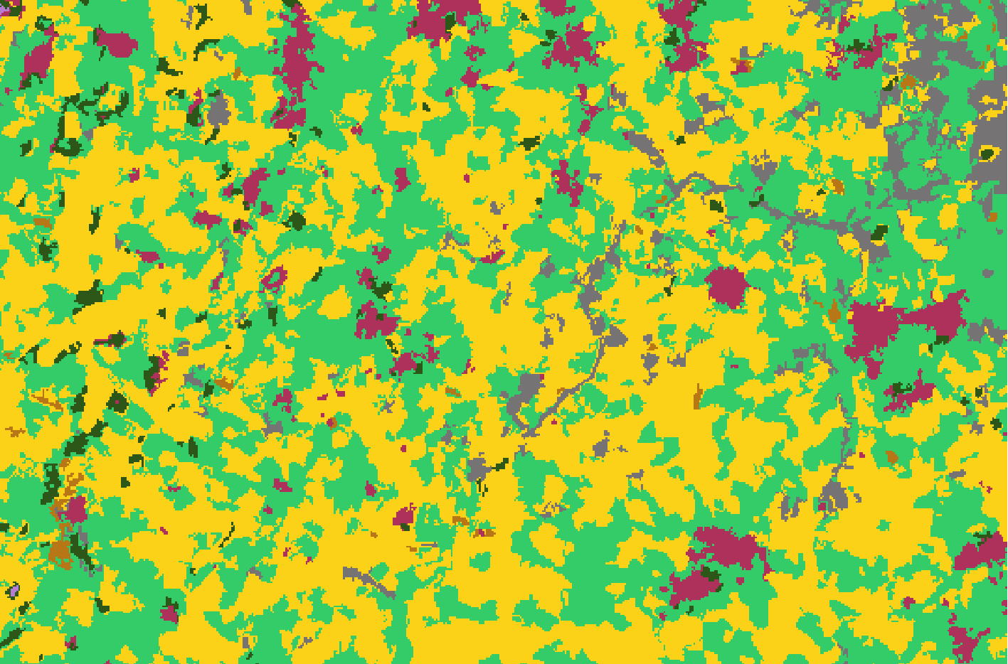
(g) RF

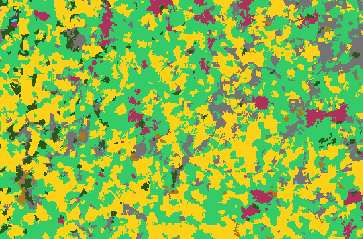
(h) SVM

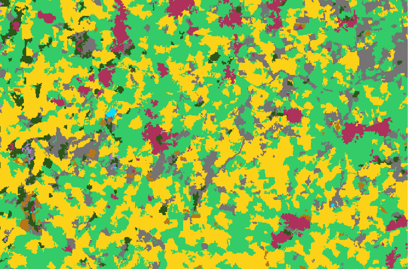
(i) MLP

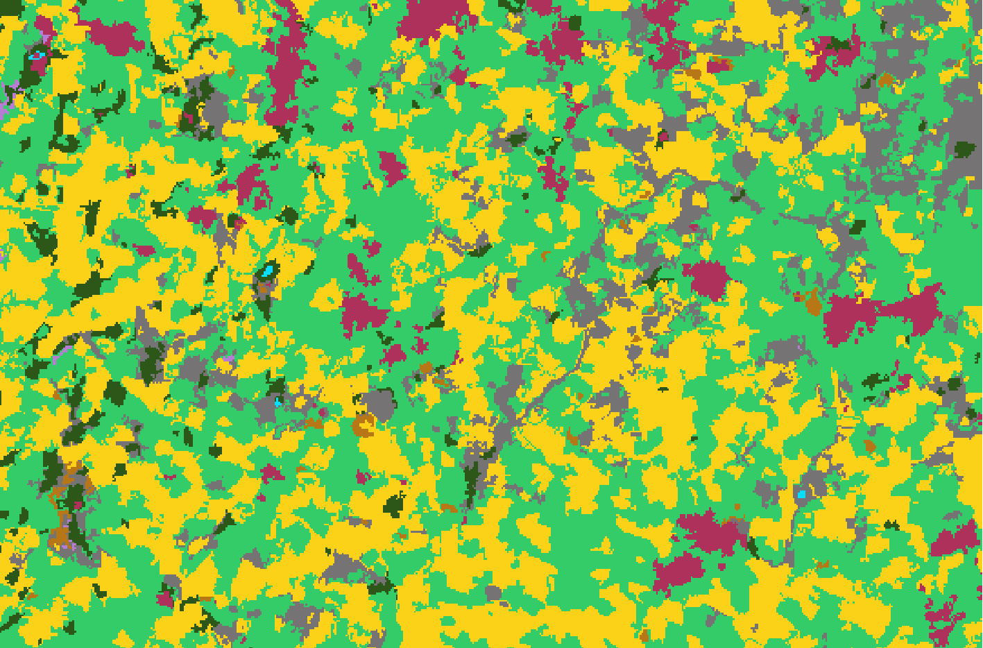
(j) HOb2sRNN

Figure 9: Qualitative investigation of land cover map details produced on the Senegalese study site by RF, SVM, MLP and HOb2sRNN on heterogeneous landscapes including buildings, agricultural and wet areas.

4.5 Attention parameters analysis

In this last part of our experimental results, we explore the side information provided by the attention mechanism introduced in Section 3.2. In order to get meaningful insights about how HOb2sRNN handles the multi-source time series for the land cover classification task. Attention weights have been successfully employed in the field of NLP [36, 38, 46] to explain which parts of the input signal contribute to the final decision of the RNN models. With the aim to set up an analogous analysis in the remote sensing time series classification context, we consider attention weights on the Senegalese site with a particular interest on crops (cereals and legumes) motivated by the agronomic knowledge we got from discussions with field experts. Recall that HOb2sRNN have learnt three sets of weights related to the attention mechanism employed to support the (auxiliary) radar, the (auxiliary) optical and the fused classifiers. To inspect the behavior of such attention mechanisms, we depict in Figures 10 and 11, the distribution of the three sets of attention weights on cereals and legumes land cover, respectively, via box plots visualizations.

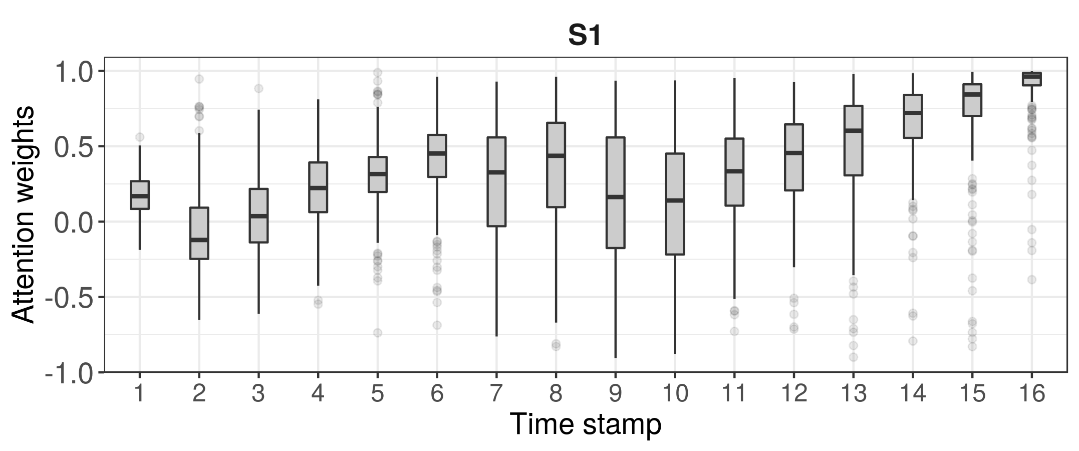
(a) Radar branch

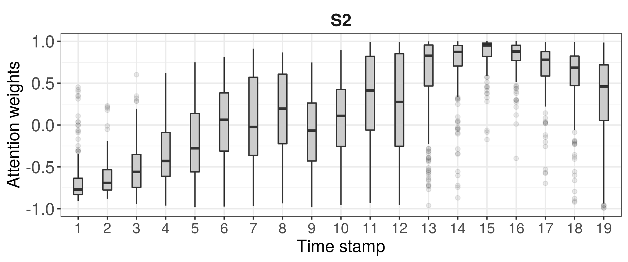
(b) Optical branch

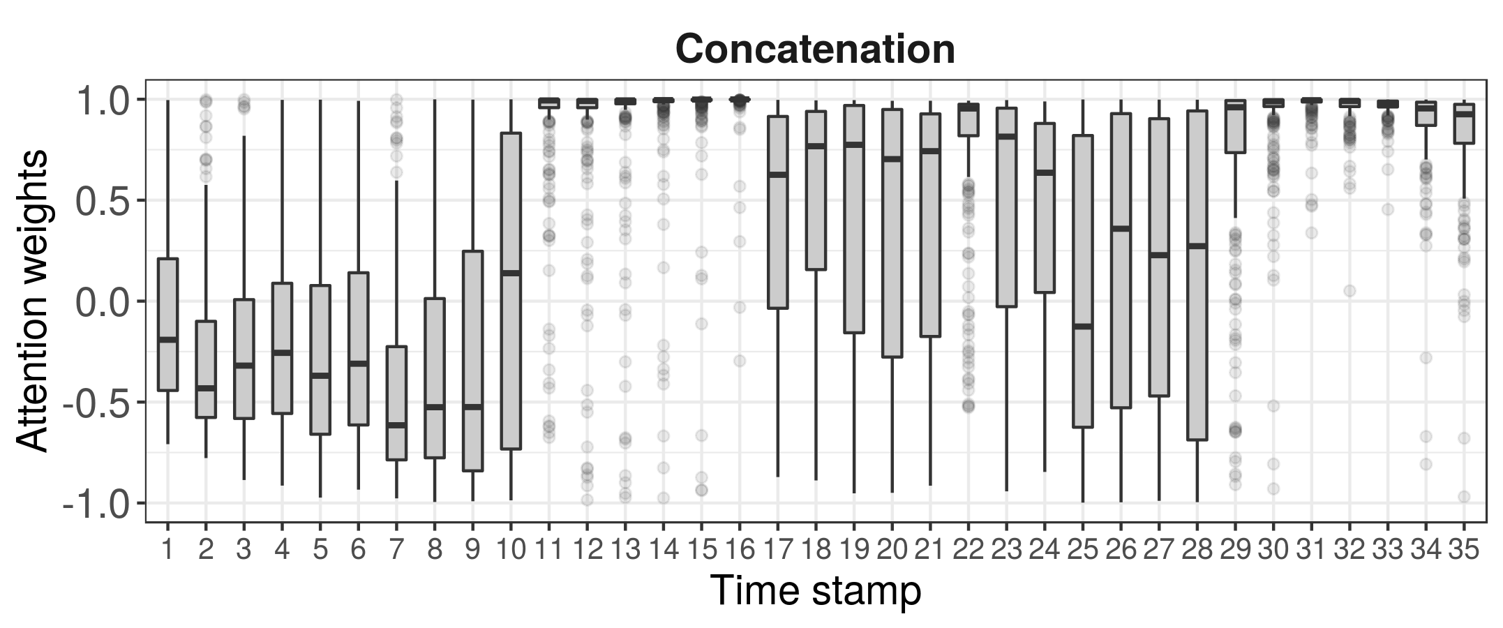
(c) Concatenated sources

Figure 10: Box plots of the Cereals class attention weights for the radar (S1) SITS (16 time stamps), the optical (S2) SITS (19 time stamps) and the concatenated sources (radar followed by optical).

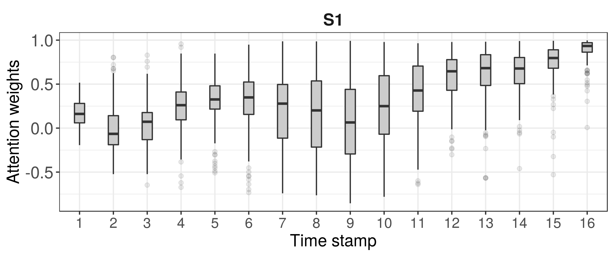
(a) Radar branch

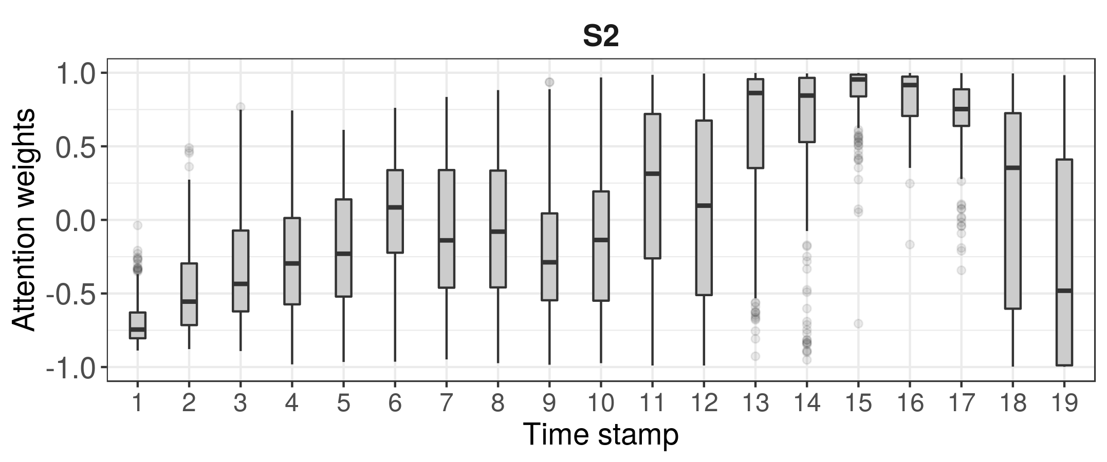
(b) Optical branch

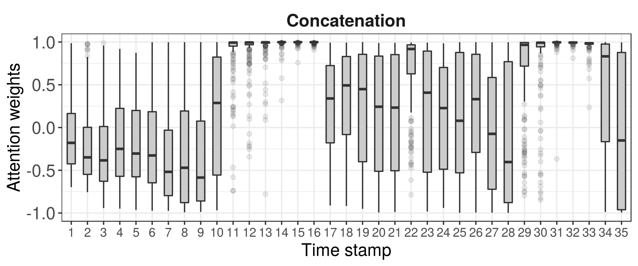
(c) Concatenated sources

Figure 11: Box plots of the Legumes class attention weights for the radar (S1) SITS (16 time stamps), the optical (S2) SITS (19 time stamps) and the concatenated sources (radar followed by optical).

At first look, we can observe that the model weights quite similarly the radar and optical time stamps on both classes. We can also notice that some time stamps towards the end of each time series are highly weighted. This behavior is especially evident on the concatenated sources distribution (Figures 10c and 11c), where high attention weights are observed from time stamp 10 (2018/08/18) for the radar SITS (ranging from 1 to 16) and time stamp 28 (2018/08/16) for the optical SITS (ranging from 17 to 35) which both correspond to the mid-August period. This is interesting to note the likely correlation existing between these high attention values and the crops growth, since in the Senegalese groundnut basin, vegetation reaches its peak activity during the August month also characterized by heavy rain amount, all inducing more differentiation among land cover classes.

However, on the two last optical time stamps (2018/10/25 and 2018/10/30), attention weights are differently attributed considering the 2 crop types. Cereals get more important attention weights for these two timestamps than legumes. This behavior seems to be associated to the agricultural practices adopted in the Senegalese groundnut basin at the end of the season. While cereals (mainly millet) are harvested cutting only the ears, legumes (mainly groundnut) are torn off. Thus, on these latter time stamps, cereal plots are covered by senescent plants while legume plots turn into bare soil. These practices are visible in the SITS and illustrated in Figure 12.

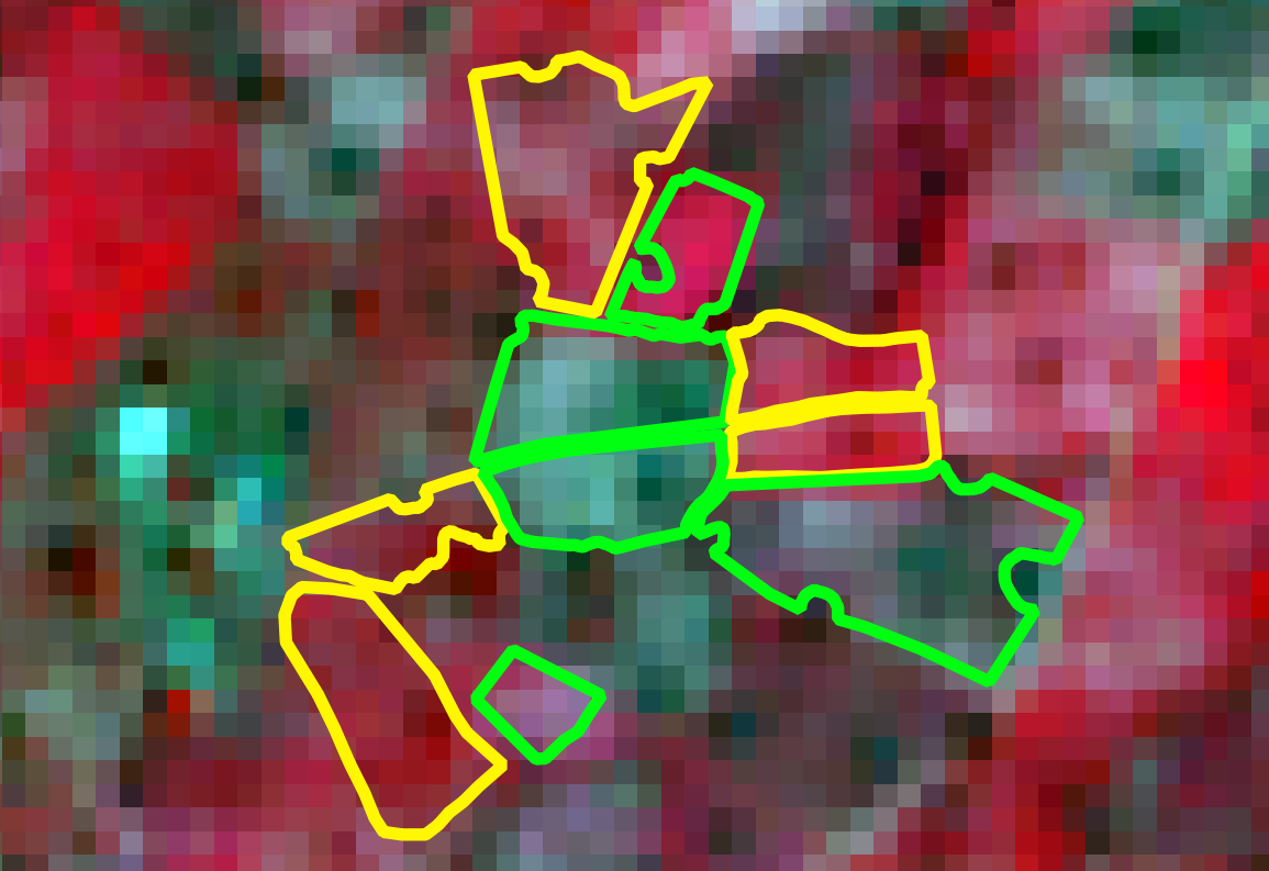
(a) 2018/10/05

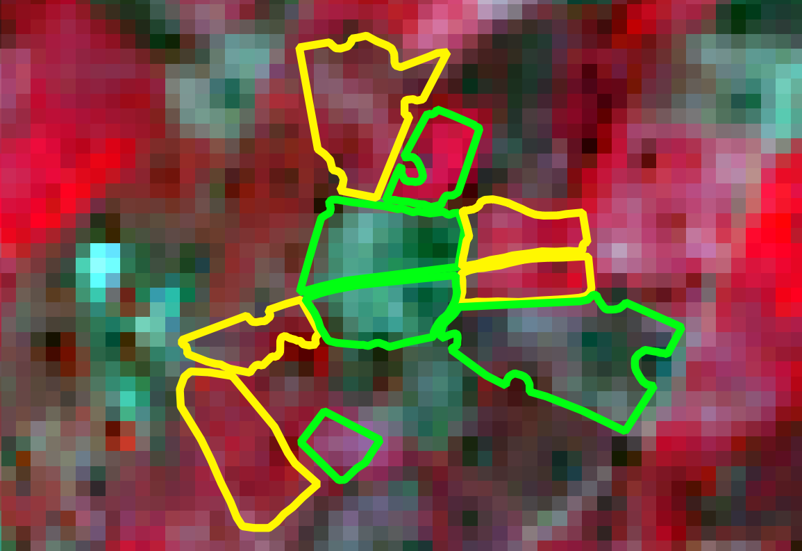
(b) 2018/10/10

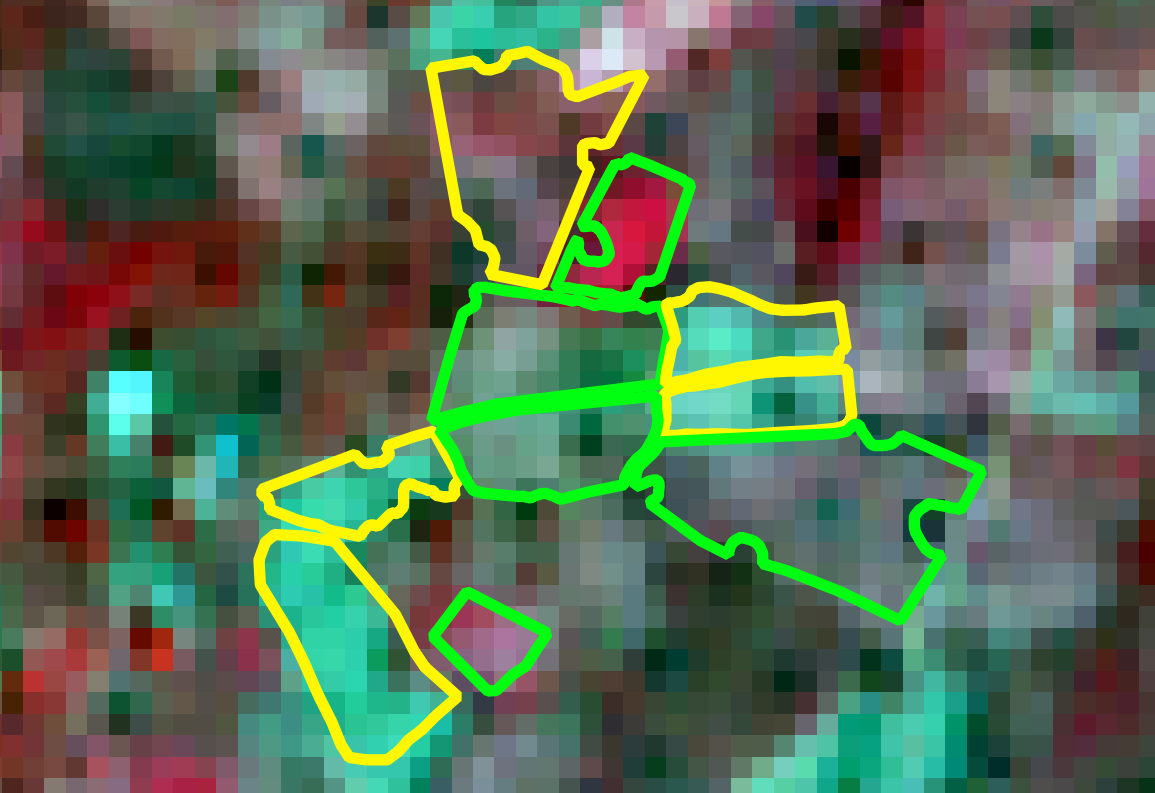
(c) 2018/10/25

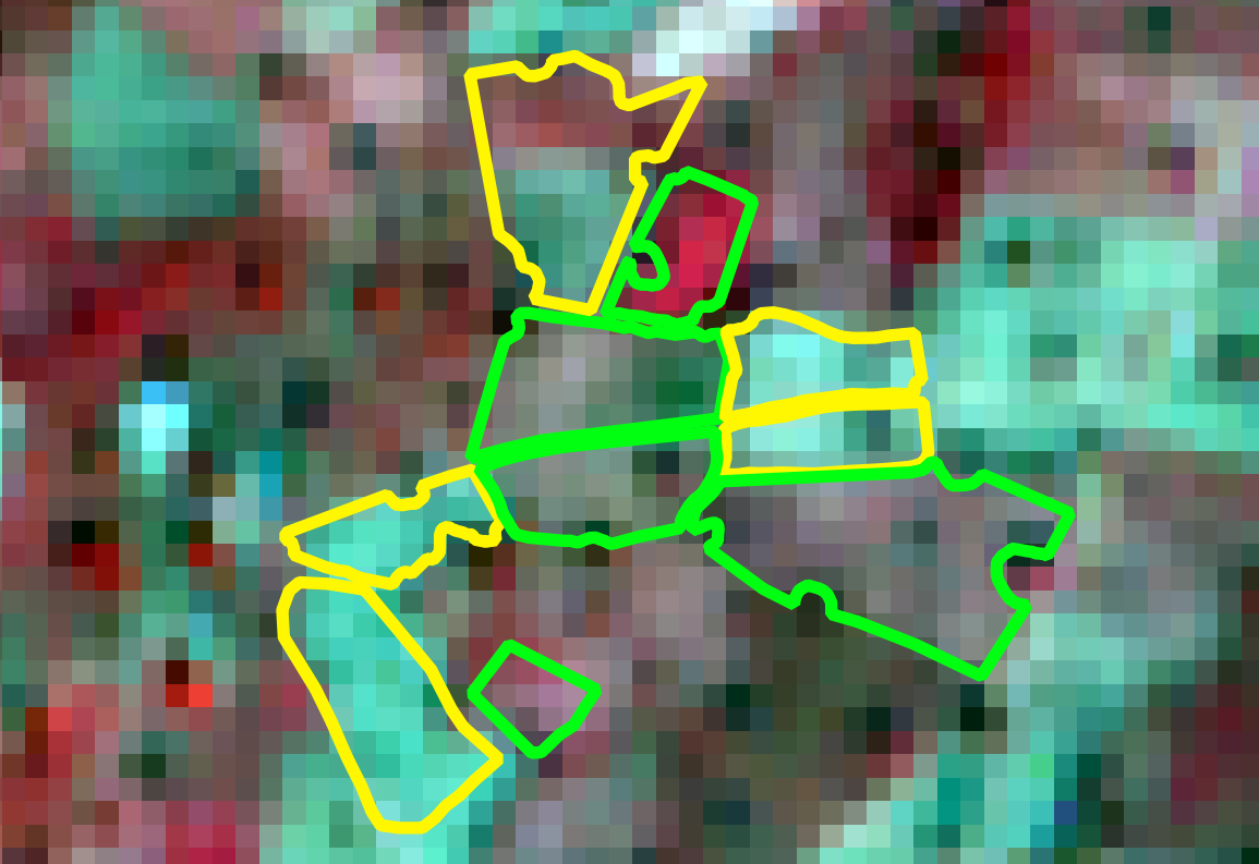
(d) 2018/10/30

(e)

Figure 12: Visualization of end of season agricultural practices in the Senegalese groundnut basin concerning cereals and legumes. Background images come from the Sentinel-2 time series and are displayed in black–Red–Infrared composite colors.

To wrap up this analysis, we have found an existing correlation between the attention weights learnt by HOb2sRNN and the informativeness of the different time stamps in the SITS data. To the best of our knowledge, no previous work exists on the exploitation of such kind of side information (attention weights) to understand and interpret the behavior of recurrent neural network models in the context of satellite image time series. As underlined by our findings, the exploration of the attention parameters can support the understanding of the decision made by our model and provides useful insights about the information contained in the SITS.

4.6 Findings summary and evaluation discussion

To summarize, the proposed deep learning framework exhibits convincing performances in land cover mapping considering situation characterized by a realistic amount of available training samples. The comparison with other machine learning approaches underlines two points: i) our approach clearly outperforms the RF classifier that is the common approach employed to deal with SITS classification and ii) other standard, less explored, machine learning methods, i.e. SVM and MLP, exhibit competitive behaviors w.r.t. our method on the study site involving the small amount of labeled samples.

The ablation study indicates that HOb2sRNN is capable to exploit the complementarity between the radar and optical information always improving its performances w.r.t. using only one of the two sources. Our framework integrates background knowledge via hierarchical pretraining leveraging taxonomic relationships between land cover classes. Experiments highlight that such knowledge seems valuable for black box models and it systematically ameliorates the behavior of HOb2sRNN. On the other hand, some other type of considered knowledge, i.e. NDVI radiometric index, seems less effective due to the fact that, probably, the model is capable to autonomously derive it. These points clearly pave the way to further investigation about which and how knowledge can be injected to guide/regularize the learning process of such techniques.

Considering model interpretability, we also conduct some qualitative studies about the side information that can be extracted from our framework. The qualitative results we obtain are in line with the agronomic knowledge on the study area. Make the black box grey is an hot topic today in the machine learning community [47] and we can state, with a certain margin of confidence, that solutions or answers associated to this question will be available in a near future.

Finally, we remind that operational/realistic constraints might be considered when dealing with remote sensing analysis. Constraints can be related to available resources, i.e. timely production of land cover maps or limited access to training samples. We are aware that, in operational/realistic scenario characterized by the, almost real-time, production of land cover maps (i.e. disaster management [48]), more computationally efficient solutions needs to be preferred (i.e. MLP or SVM) to deep learning approaches. On the other hand, in our work we deal with (agricultural-oriented) land cover mapping where, land cover maps need to be provided with a relative low time frequency (once or twice per year). Due to this fact, here, the operational constraints are mainly intended regarding the limited amount of available labeled samples. In such data paucity setting, our approach clearly outperforms the Random Forest classifier, that is the de facto strategy involved in the classification of SITS data [49]. In addition, the experimental evaluation pointed out that, less explored machine learning techniques, in the context of SITS analysis, i.e. SVM and MLP, deserve much attention since they constitute valuable strategies to which compare future proposals.

5 Conclusion

In this work, we propose to deal with land cover mapping at object level, from multi-temporal and multi-source (radar and optical) data. Our approach is based on an extension of RNN involving a modified attention mechanism devised to better suit the SITS data context. We also introduce a novel hierarchical pretraining approach for neural networks which integrates specific knowledge from land cover classes to support the land cover mapping task. Extensive quantitative and qualitative evaluations on two different study sites demonstrate the effectiveness of the proposal compared to common and not common machine learning techniques in the field of land cover mapping. As future work, we plan to investigate other deep learning approaches conceived to better deal with sequential (temporal) data than RNN namely transformers [50] or one dimensional convolutional neural networks [51] also tailored to process this kind of data. In addition, a possible extension of the actual framework could be done towards leveraging spatial dependencies in the multi-source SITS via convolutions.

References

- [1] M. Berger, J. Moreno, J. A. Johannessen, P. F. Levelt, R. F. Hanssen, Esa’s sentinel missions in support of earth system science, Remote Sensing of Environment 120 (2012) 84 – 90.
- [2] N. Kolecka, C. Ginzler, R. Pazur, B. Price, P. H. Verburg, Regional scale mapping of grassland mowing frequency with sentinel-2 time series, Remote Sensing 10 (8) (2018) 1221.
- [3] N. Kussul, M. Lavreniuk, S. Skakun, A. Shelestov, Deep learning classification of land cover and crop types using remote sensing data, IEEE Geosci. Remote Sensing Lett. 14 (5) (2017) 778–782.
- [4] J. Inglada, A. Vincent, M. Arias, B. Tardy, D. Morin, I. Rodes, Operational high resolution land cover map production at the country scale using satellite image time series, Remote Sensing 9 (1) (2017) 95.
- [5] F. Guttler, D. Ienco, J. Nin, M. Teisseire, P. Poncelet, A graph-based approach to detect spatiotemporal dynamics in satellite image time series, ISPRS J. of Photogr. and Rem. Sens. 130 (2017) 92–107.
- [6] L. Khiali, D. Ienco, M. Teisseire, Object-oriented satellite image time series analysis using a graph-based representation, Ecological Informatics 43 (2018) 52–64.
- [7] M. J. Steinhausen, P. D. Wagner, B. Narasimhan, B. Waske, Combining sentinel-1 and sentinel-2 data for improved land use and land cover mapping of monsoon regions, International Journal of Applied Earth Observation and Geoinformation 73 (2018) 595 – 604.
- [8] D. H. T. Minh, D. Ienco, R. Gaetano, N. Lalande, E. Ndikumana, F. Osman, P. Maurel, Deep recurrent neural networks for winter vegetation quality mapping via multitemporal sar sentinel-1, IEEE Geosc. and Rem. Sens. Letters Preprint (-) (2018) –.
- [9] Y. J. E. Gbodjo, D. Ienco, L. Leroux, Toward Spatio-Spectral Analysis of Sentinel-2 Time Series Data for Land Cover Mapping, IEEE Geoscience and Remote Sensing Letters (2019) 1–5.
- [10] R. Interdonato, D. Ienco, R. Gaetano, K. Ose, Duplo: A dual view point deep learning architecture for time series classification, ISPRS Journal of Photogrammetry and Remote Sensing 149 (2019) 91 – 104.
- [11] S. M. Mousavi, S. roostaei, H. Rostamzadeh, Estimation of flood land use/land cover mapping by regional modelling of flood hazard at sub-basin level case study: Marand basin, Geomatics, Natural Hazards and Risk 10 (1) (2019) 1155–1175.
- [12] S. Fritz, L. See, J. C. L. Bayas, F. Waldner, D. Jacques, I. Becker-Reshef, A. Whitcraft, B. Baruth, R. Bonifacio, J. Crutchfield, F. Rembold, O. Rojas, A. Schucknecht, M. V. der Velde, J. Verdin, B. Wu, N. Yan, L. You, S. Gilliams, S. Mücher, R. Tetrault, I. Moorthy, I. McCallum, A comparison of global agricultural monitoring systems and current gaps, Agricultural Systems 168 (2019) 258 – 272.
- [13] F. Gao, J. G. Masek, M. R. Schwaller, F. G. Hall, On the blending of the landsat and MODIS surface reflectance: predicting daily landsat surface reflectance, IEEE Trans. Geoscience and Remote Sensing 44 (8) (2006) 2207–2218.
- [14] D. Ienco, R. Interdonato, R. Gaetano, D. H. T. Minh, Combining sentinel-1 and sentinel-2 satellite image time series for land cover mapping via a multi-source deep learning architecture, ISPRS Journal of Photogrammetry and Remote Sensing 158 (2019) 11 – 22.
- [15] G. C. Iannelli, P. Gamba, Jointly exploiting sentinel-1 and sentinel-2 for urban mapping, in: 2018 IEEE International Geoscience and Remote Sensing Symposium, IGARSS 2018, Valencia, Spain, July 22-27, 2018, 2018, pp. 8209–8212.
- [16] R. C. Sharma, K. Hara, R. Tateishi, Developing forest cover composites through a combination of landsat-8 optical and sentinel-1 SAR data for the visualization and extraction of forested areas, J. Imaging 4 (9) (2018) 105.
- [17] R. Fernández-Beltran, J. M. Haut, M. E. Paoletti, J. Plaza, A. Plaza, F. Pla, Multimodal probabilistic latent semantic analysis for sentinel-1 and sentinel-2 image fusion, IEEE Geosci. Remote Sensing Lett. 15 (9) (2018) 1347–1351.
- [18] J. Erinjery, M. Singh, R. Kent, Mapping and assessment of vegetation types in the tropical rainforests of the western ghats using multispectral sentinel-2 and sar sentinel-1 satellite imagery, Remote Sensing of Environment 216 (2018) 345–354.
- [19] K. V. Tricht, A. Gobin, S. Gilliams, I. Piccard, Synergistic use of radar sentinel-1 and optical sentinel-2 imagery for crop mapping: A case study for belgium, Remote Sensing 10 (10) (2018) 1642.
- [20] A. Di Gregorio, Land cover classification system: classification concepts and user manual: LCCS, Vol. 2, Food & Agriculture Org., 2005.
- [21] D. Sulla-Menashe, M. A. Friedl, O. N. Krankina, A. Baccini, C. E. Woodcock, A. Sibley, G. Sun, V. Kharuk, V. Elsakov, Hierarchical mapping of northern eurasian land cover using modis data, Remote Sensing of Environment 115 (2) (2011) 392 – 403.
- [22] M. F. Wu, Z. C. Sun, B. Yang, S. S. Yu, A hierarchical object-oriented urban land cover classification using WorldView-2 imagery and airborne LiDAR data, IOP Conference Series: Earth and Environmental Science 46.
- [23] D. Sulla-Menashe, J. M. Gray, S. P. Abercrombie, M. A. Friedl, Hierarchical mapping of annual global land cover 2001 to present: The modis collection 6 land cover product, Remote Sensing of Environment 222 (2019) 183 – 194.
- [24] T. Blaschke, Object based image analysis for remote sensing, ISPRS journal of photogrammetry and remote sensing 65 (1) (2010) 2–16.
- [25] T. Lillesand, R. W. Kiefer, J. Chipman, Remote sensing and image interpretation, John Wiley & Sons, 2015.
- [26] X. Zhu, D. Tuia, L. Mou, G. X. L. Zhang, F. Xu, F. Fraundorfer, Deep learning in remote sensing: A comprehensive review and list of resources, IEEE Geosci. Remote Sens. Mag. 5 (2017) 8–36.
- [27] D. Ienco, R. Gaetano, C. Dupaquier, P. Maurel, Land cover classification via multitemporal spatial data by deep recurrent neural networks, IEEE Geosc. and Rem. Sens. Letters 14 (10) (2017) 1685–1689.
- [28] L. Mou, P. Ghamisi, X. X. Zhu, Unsupervised spectral-spatial feature learning via deep residual conv-deconv network for hyperspectral image classification, IEEE Trans. Geoscience and Remote Sensing 56 (1) (2018) 391–406.
- [29] L. Zhong, L. Hu, H. Zhou, Deep learning based multi-temporal crop classification, Remote Sensing of Environment 221 (2019) 430–443.
- [30] J. W. Rouse, R. H. Haas, J. A. Schell, D. Deering, Monitoring the vernal advancement and retrogradation (green wave effect) of natural vegetation, Progress Report RSC 1978-1 (1973) 112.
- [31] P. Lassalle, J. Inglada, J. Michel, M. Grizonnet, J. Malik, A scalable tile-based framework for region-merging segmentation, IEEE Trans. on Geosc. and Rem. Sens. 53 (10) (2015) 5473–5485.
- [32] K. Cho, B. van Merrienboer, Ç. Gülçehre, D. Bahdanau, F. Bougares, H. Schwenk, Y. Bengio, Learning phrase representations using RNN encoder-decoder for statistical machine translation, in: EMNLP, 2014, pp. 1724–1734.
- [33] S. Hochreiter, J. Schmidhuber, LSTM can solve hard long time lag problems, in: NIPS, 1996, pp. 473–479.
- [34] P. Benedetti, D. Ienco, R. Gaetano, K. Ose, R. G. Pensa, S. Dupuy, M3 fusion: A deep learning architecture for multiscale multimodal multitemporal satellite data fusion, IEEE J. of Sel. Topics in Applied Earth Obs. and Rem. Sens. 11 (12) (2018) 4939–4949.
- [35] L. Mou, P. Ghamisi, X. X. Zhu, Deep recurrent neural networks for hyperspectral image classification, IEEE Trans. on Geosc. and Rem. Sens. 55 (7) (2017) 3639–3655.
- [36] D. Bahdanau, K. Cho, Y. Bengio, Neural machine translation by jointly learning to align and translate, arXiv:1409.0473 [cs, stat] (2014) 1–15.
- [37] M. Luong, H. Pham, C. D. Manning, Effective approaches to attention-based neural machine translation, in: Proceedings of the 2015 Conference on Empirical Methods in Natural Language Processing, EMNLP 2015, 2015, pp. 1412–1421.
- [38] D. Britz, M. Y. Guan, M. Luong, Efficient attention using a fixed-size memory representation, in: EMNLP, 2017, pp. 392–400.
- [39] I. Sutskever, O. Vinyals, Q. V. Le, Sequence to sequence learning with neural networks, in: Advances in Neural Information Processing Systems 27: Annual Conference on Neural Information Processing Systems 2014, 2014, pp. 3104–3112.
- [40] S. Hou, X. Liu, Z. Wang, Dualnet: Learn complementary features for image recognition, in: ICCV, 2017, pp. 502–510.
- [41] F. Pedregosa, G. Varoquaux, A. Gramfort, V. Michel, B. Thirion, O. Grisel, M. Blondel, P. Prettenhofer, R. Weiss, V. Dubourg, J. Vanderplas, A. Passos, D. Cournapeau, M. Brucher, M. Perrot, E. Duchesnay, Scikit-learn: Machine learning in Python, Journal of Machine Learning Research 12 (2011) 2825–2830.
- [42] D. P. Kingma, J. Ba, Adam: A method for stochastic optimization, CoRR abs/1412.6980.
- [43] Y. Lecun, Y. Bengio, G. Hinton, Deep learning, Nature 521 (7553) (2015) 436–444.
- [44] L. Ma, Y. Liu, X. Zhang, Y. Ye, G. Yin, B. A. Johnson, Deep learning in remote sensing applications: A meta-analysis and review, ISPRS Journal of Photogrammetry and Remote Sensing 152 (April) (2019) 166–177.
- [45] A. E. Maxwell, T. A. Warner, F. Fang, Implementation of machine-learning classification in remote sensing: an applied review, International Journal of Remote Sensing 39 (9) (2018) 2784–2817.
- [46] H. Choi, K. Cho, Y. Bengio, Fine-grained attention mechanism for neural machine translation, Neurocomputing 284 (2018) 171–176.
- [47] M. T. Ribeiro, S. Singh, C. Guestrin, ”why should I trust you?”: Explaining the predictions of any classifier, in: Proceedings of the 22nd ACM SIGKDD International Conference on Knowledge Discovery and Data Mining, San Francisco, CA, USA, August 13-17, 2016, 2016, pp. 1135–1144.
- [48] P. Boccardo, F. G. Tonolo, Remote sensing role in emergency mapping for disaster response, in: Engineering Geology for Society and Territory-Volume 5, Springer, 2015, pp. 17–24.
- [49] M. Belgiu, L. Drăguţ, Random forest in remote sensing: A review of applications and future directions, ISPRS Journal of Photogrammetry and Remote Sensing 114 (2016) 24 – 31.
- [50] A. Vaswani, N. Shazeer, N. Parmar, J. Uszkoreit, L. Jones, A. N. Gomez, L. Kaiser, I. Polosukhin, Attention is all you need, in: Advances in Neural Information Processing Systems 30: Annual Conference on Neural Information Processing Systems 2017, 4-9 December 2017, Long Beach, CA, USA, 2017, pp. 5998–6008.
- [51] C. Pelletier, G. Webb, F. Petitjean, Temporal convolutional neural network for the classification of satellite image time series, Remote Sensing 11 (5) (2019) 523.