Network Flows that Solve Sylvester Matrix Equations

Abstract

In this paper, we study distributed methods for solving a Sylvester equation in the form of $\mathbf{A}\mathbf{X}+\mathbf{X}\mathbf{B}=\mathbf{C}$ for matrices $\mathbf{A},\mathbf{B},\mathbf{C}\in\mathbb{R}^{n\times n}$ with $\mathbf{X}$ being the unknown variable. The entries of $\mathbf{A},\mathbf{B}$ and $\mathbf{C}$ (called data) are partitioned into a number of pieces (or sometimes we permit these pieces to overlap). Then a network with a given structure is assigned, whose number of nodes is consistent with the partition. Each node has access to the corresponding set of data and holds a dynamic state. Nodes share their states among their neighbors defined from the network structure, and we aim to design flows that can asymptotically converge to a solution of this equation. The decentralized data partitions may be resulted directly from networks consisting of physically isolated subsystems, or indirectly from artificial and strategic design for processing large data sets. Natural partial row/column partitions, full row/column partitions and clustering block partitions of the data $\mathbf{A},\mathbf{B}$ and $\mathbf{C}$ are assisted by the use of the vectorized matrix equation. We show that the existing “consensus $+$ projection” flow and the “local conservation $+$ global consensus” flow for distributed linear algebraic equations can be used to drive distributed flows that solve this kind of equations. A “consensus $+$ projection $+$ symmetrization” flow is also developed for equations with symmetry constraints on the solution matrices. We reveal some fundamental convergence rate limitations for such flows regardless of the choices of node interaction strengths and network structures. For a special case with $\mathbf{B}=\mathbf{A}^{T}$, where the equation mentioned is reduced to a classical Lyapunov equation, we demonstrate that by exploiting the symmetry of data, we can obtain flows with lower complexity for certain partitions.

Keywords: Distributed algorithms; matrix equations; network flows; convergence rate.

1 Introduction

Recently, distributed optimization and computation in multi-agent networks have received growing research interest, where applications are witnessed in various problems for the control and operation of large-scale network systems [1, 2]. A number of distributed algorithms have arisen, involving many fields such as distributed control and estimation, and distributed signal processing [3, 4, 5]. A related problem with growing research attention is to design distributed algorithms for solving the linear algebraic equation $\mathbf{A}\mathbf{x}=\mathbf{b}$ over a given network where the rows of $\mathbf{A}$ and the entries of $\mathbf{b}$ are allocated to individual nodes. These distributed optimization and computation ideas have also been explored in the areas of parallel computation and machine learning [6, 7], while efforts under the multi-agent frameworks focus more on scalability and resilience advantages for a given network structure.

As for the linear equation $\mathbf{A}\mathbf{x}=\mathbf{b}$, there are a few distributed solutions as discrete-time or continuous-time algorithms over networks [8, 9, 10, 11, 12, 13, 14]. Every node only knows local information, such as one or several rows of $\mathbf{A}$ and $\mathbf{b}$, and then communicates with its neighbors about a dynamically evolving state. As long as $\mathbf{A}\mathbf{x}=\mathbf{b}$ has at least one solution, finding a solution to the original equation is equivalent to finding a solution in the intersection of affine subspaces defined by the solution spaces of individual nodes. With proper design of distributed flows, nodes can asymptotically agree on a certain solution to the overall equation $\mathbf{A}\mathbf{x}=\mathbf{b},$ complying with a given network structure and only exchanging state information (as opposed to information about $\mathbf{A}$ and $\mathbf{b}$). Notably, the “consensus + projection” flow [12] has a simple form consisting of a standard consensus term and a local projection term onto every individual affine subspace. Generalized high-order flows with consensus and projection can even solve the equation approximately in the least-squares sense [12]. In addition, a double-layer network has been proposed to allow for a general data partition of the entries in $\mathbf{A}$ and $\mathbf{b}$, where the “local conservation + global consensus” flow [13] or its variation can be used to solve $\mathbf{A}\mathbf{x}=\mathbf{b}$ distributively.

Linear matrix equations, which are particular forms of structured linear equations, appear in various fields of science and engineering [15, 16, 17], such as the Sylvester equation in the form of $\mathbf{A}\mathbf{X}+\mathbf{X}\mathbf{B}=\mathbf{C}$ with $\mathbf{A}\in\mathbb{R}^{n\times n},\mathbf{B}\in\mathbb{R}^{m\times m},\mathbf{C}\in\mathbb{R}^{n\times m}$ and the unknown $\mathbf{X}\in\mathbb{R}^{n\times m}$. In fact, many Sylvester-type matrix equations in the control and automation areas serve as basic models for lots of fundamental systems and problems. For example, the Sylvester equation can be used to achieve pole/eigenstructure assignment by designing a controller for mechanical vibrating systems [18], while the Lyapunov equation with $\mathbf{B}=\mathbf{A}^{T}$ plays an essential role in studying the stability of linear time-invariant systems [19]. The motivation for study distributed solver for Sylvester equations may come from the following two aspects: (i) Extension for linear algebraic equations to matrix equations is nontrivial, because the data partitions of entries in $(\mathbf{A},\mathbf{B},\mathbf{C})$ complying with a network would lead to fundamentally different computing problems compared to a standard linear algebraic equation; (ii) Increasing growing study of complex network systems requires distributed solutions of the matrix equations from physically isolated data sets to problems as basic as stability validation.

In this paper, we concentrate on seeking a solution to the matrix equation $\mathbf{A}\mathbf{X}+\mathbf{X}\mathbf{B}=\mathbf{C}$ with $\mathbf{A},\mathbf{B},\mathbf{C},\mathbf{X}\in\mathbb{R}^{n\times n}$ in a distributed way. Here we choose to work on square matrices to facilitate a simplified presentation; nonetheless, our methods and analysis can be straightforwardly generalized to the general Sylvester equation with $\mathbf{X}\in\mathbb{R}^{n\times m}$, because $\mathbf{X}$ being a square matrix plays no role in our algorithm design and convergence characterizations. Note that the system cannot be directly studied with the methods for the equation $\mathbf{A}\mathbf{X}\mathbf{B}=\mathbf{F}$ discussed in [20] because these two equations necessarily give rise to different patterns of assignment of data to network nodes. The work [20] builds a solution procedure from an optimization perspective and solves several primal and dual optimization problems via distributed methods, while we plan to transform matrix equations by vectorization and take advantage of the above referenced distributed algorithms for solving $\mathbf{A}\mathbf{x}=\mathbf{b}$. More concretely, in our design, each node has access to local data in matrices $\mathbf{A},\mathbf{B}$ and $\mathbf{C}$ with the following several partition patterns, which may be suited to certain different problems.

• [Partial row/column partition] E.g., for an $n$-node network, each node $i$ holds the $i$-th column of $\mathbf{B}$ and $\mathbf{C}$, with the entire $\mathbf{A}$ known to the whole network. We show that with such partition, we can utilize the “consensus $+$ projection” flow for an $n$-node network, under which we establish convergence with an explicit rate and more interestingly, a rate limitation characterization of the flow. In addition, we design a “consensus $+$ projection $+$ symmetrization” flow for symmetry constraints on the solution matrices, followed by its properties of convergence and rate limitation.

• [Full row/column partition] E.g., for an $n$-node network, each node $i$ holds the $i$-th row of $\mathbf{A}$, and the $i$-th column of $\mathbf{B}$ and $\mathbf{C}$. We show that under this type of partition, the Sylvester equation can be solved distributedly by introducing an auxiliary variable and taking advantage of an augmented “consensus + projection” flow in a node state space with dimension $n^{2}(1+n)$.

• [Clustering block partition] E.g., for a double-layer network with $n$ clusters, the $i$-th of which having $n$ nodes holds the entire $\mathbf{A}$, and the $i$-th column of $\mathbf{B}$ and $\mathbf{C}$, where each node $j$ within cluster $i$ is assigned to the $(j,i)$-th entry of $\mathbf{B}$ and $\mathbf{C}$, and additional matrix $\mathbf{A}$ if $j=i$. Taking advantage of the “local conservation $+$ global consensus” flow, we establish convergence with an explicit rate as well. As a byproduct of the study, a fundamental property of the convergence rate in the “local conservation $+$ global consensus” flow is also established, which is of independent interest.

In a brief discussion, we also show that the data $\mathbf{A},\mathbf{B}$ and $\mathbf{C}$ can be partitioned over an $n^{2}$-node network, where each node holds one row of $\mathbf{A}$, one column of $\mathbf{B}$ and one entry of $\mathbf{C}$. As a result, the data complexity at each node is reduced with $n^{2}$ nodes, while the rate of convergence for the resulting flow, however, becomes lower due to the increased network size. If in addition, there is a particular case with $\mathbf{B}=\mathbf{A}^{T}$, where the equation becomes a Lyapunov equation, and by exploiting the symmetry, the size of nodes can be reduced to $n(n+1)/2$ compared with the $n^{2}$-node network.

For this paper, the remainder is organized as follows. In Section 2, we define the considered matrix equation problem with a motivating example. In Section 3, we present a network flow with partial row/column partitions and prove the convergence rate limitation, followed by some numerical examples and discussions. We consider full row/column partitions in Section 4 with corresponding network flow. In Section 5, we present a network flows with a clustering block partition and set out some properties. In Section 6, we conclude the paper briefly with a few remarks. Finally, some useful results related to linear algebra, projection, and exponential stability are introduced in Appendix A, and other details of proofs are given in subsequent appendices.

Notation: Let $\mathbf{0}$ or $\mathbf{1}$ represent the matrix (or vector) with all entries being $0$ or $1$, and their dimensions are indicated by subscripts. Let $\mathbf{I}_{n}$ denote an $n$ by $n$ identity matrix and $\mathbf{e}_{i}$ denote the $i$-th column vector of $\mathbf{I}_{n}.$ Let $\mathrm{col}\{\mathbf{M}_{[1]},\cdots,\mathbf{M}_{[n]}\}=[\mathbf{M}_{[1]}^{T},\cdots,\mathbf{M}_{[n]}^{T}]^{T}$ be a stack of matrices $\mathbf{M}_{[i]},i=1,\cdots,n$. Let $\mathrm{vec}_{mn}(\cdot)$ be a mapping from $\mathbb{R}^{m\times n}$ to $\mathbb{R}^{mn}$: $\mathrm{vec}(\mathbf{A})=\mathrm{col}\{\mathbf{A}_{1},\cdots,\mathbf{A}_{n}\}$ with $\mathbf{A}_{i}$ being the $i$-th column of $\mathbf{A}.$ The inverse mapping of $\mathrm{vec}_{mn}(\cdot)$ can be well-defined, which is denoted by $\mathrm{vec}_{mn}^{-1}(\cdot)$. The subscripts of $\mathrm{vec}_{mn}(\cdot)$ and $\mathrm{vec}_{mn}^{-1}(\cdot)$ would be dropped whenever there is no ambiguity of the space dimensions. Denote by $\mathrm{span}(\mathbf{M}),\ker(\mathbf{M})$ and $\mathrm{rank}(\mathbf{M})$, the column space, the kernel space and the rank of a matrix $\mathbf{M}$, respectively. Let $\mathrm{diag}\{\mathbf{F}_{[1]},\cdots,\mathbf{F}_{[n]}\}$ denote the block diagonal matrix with sub-blocks $\mathbf{F}_{[i]},i=1,\cdots,n$. For a matrix $\mathbf{A}\in\mathbb{R}^{n\times n}$ with all real eigenvalues, let $\mathrm{spec}(\mathbf{A})=\{\lambda_{1}(\mathbf{A}),\cdots,\lambda_{n}(\mathbf{A})\}$ denote the set of all the eigenvalues of $\mathbf{A}$ with $\lambda_{1}(\mathbf{A})\geq\lambda_{2}(\mathbf{A})\geq\cdots\geq\lambda_{n}(\mathbf{A})$. Let $\otimes$ denote the Kronecker product and $\mathrm{dim}(\mathcal{V})$ represent the dimension of a subspace $\mathcal{V}$ in $\mathbb{R}^{n}.$ Let $\|\cdot\|(\|\cdot\|_{F})$ denote the Euclidean (Frobenius) norm of a vector (matrix) and $B_{\delta}:=\{\mathbf{x}\in\mathbb{R}^{n}:\|\mathbf{x}\|\leq\delta\}$ denote the closed ball with radius $\delta$ and center at the origin. Denote a network graph $\mathrm{G}=(\mathrm{V},\mathrm{E})$ with node set $\mathrm{V}$ and edge set $\mathrm{E}.$ All graphs in the remainder of this paper are connected and undirected. The neighbor set of node $i$ is given by $\mathrm{N}_{i}:=\{j:(i,j)\in\mathrm{E}\}$, from which the node $i$ can receive information. Introduce $\mathbf{A}_{\mathrm{G}}$ as the adjacency matrix of $\mathrm{G},$ with $[\mathbf{A}_{\mathrm{G}}]_{ij}=1$ if $(i,j)\in\mathrm{E},$ and $[\mathbf{A}_{\mathrm{G}}]_{ij}=0,$ otherwise. The Laplacian matrix $\mathbf{L}_{\mathrm{G}}$ associated with $\mathrm{G}$ is defined by $\mathbf{L}_{\mathrm{G}}=\mathbf{D}_{\mathrm{G}}-\mathbf{A}_{\mathrm{G}},$ where $\mathbf{D}_{\mathrm{G}}=\mathrm{diag}\{\sum_{j\in\mathrm{N}_{i}}[\mathbf{A}_{\mathrm{G}}]_{ij},i\in\mathrm{V}\}$ is the degree matrix of the graph $\mathrm{G}$.

2 Problem Definition

In this section, we introduce the motivation of the study for matrix equations over networks and define the problem of interest.

2.1 Matrix Equation

Consider a matrix equation with respect to variable $\mathbf{X}\in\mathbb{R}^{n\times n}$:

$$\mathbf{A}\mathbf{X}+\mathbf{X}\mathbf{B}=\mathbf{C},\quad\mathbf{A},\mathbf{B},\mathbf{C}\in\mathbb{R}^{n\times n}.$$ (1)

By vectorization, we have the following equivalent equation of (1)

$$(\mathbf{I}_{n}\otimes\mathbf{A}+\mathbf{B}^{T}\otimes\mathbf{I}_{n})\mathbf{x}=\mathbf{c},$$ (2)

where $\mathbf{x}=\mathrm{vec}(\mathbf{X}),\mathbf{c}=\mathrm{vec}(\mathbf{C})$. There are three cases covering the solvability properties.

1. The solution to $\eqref{eq:olinear_equation}$ is unique if and only if the matrix $\mathbf{I}_{n}\otimes\mathbf{A}+\mathbf{B}^{T}\otimes\mathbf{I}_{n}$ is nonsingular, which is equivalent to $\mathrm{spec}(\mathbf{A})\cap\mathrm{spec}(-\mathbf{B})=\emptyset$ [21].

2. The solution to $\eqref{eq:olinear_equation}$ is an infinite set when $\mathrm{spec}(\mathbf{A})\cap\mathrm{spec}(-\mathbf{B})\neq\emptyset$ and $\mathbf{c}\in\mathrm{span}(\mathbf{I}_{n}\otimes\mathbf{A}+\mathbf{B}^{T}\otimes\mathbf{I}_{n}).$

3. There is no exact solutions to (2) when $\mathbf{c}\notin\mathrm{span}(\mathbf{I}_{n}\otimes\mathbf{A}+\mathbf{B}^{T}\otimes\mathbf{I}_{n}).$

2.2 A Motivating Example

Consider the following network system with $n$ dynamically coupled subsystems, for $i\in\mathrm{V}=\{1,\cdots,n\}$:

$$\dot{\mathbf{y}}_{i}=\mathbf{D}_{ii}\mathbf{y}_{i}+\sum_{j=1,j\neq i}^{n}\mathbf{D}_{ij}\mathbf{y}_{j},\quad\mathbf{D}_{ij}\in\mathbb{R}^{m\times m},\mathbf{y}_{i}\in\mathbb{R}^{m},$$ (3)

where $\mathbf{y}_{i}$ is the state of the subsystem $i$ and $\mathbf{D}_{ij}$ represents the dynamical influence from subsystem $j$ to subsystem $i$. The system (3) is arguably one of the most basic models for dynamical networks with linear couplings, which may represent a large number of practical network systems ranging from power distribution, transportation, and controlled formation [22, 23, 24, 25, 26]. The overall network dynamics is in the form of $\dot{\mathbf{y}}(t)=\mathbf{A}\mathbf{y}(t)$, where $\mathbf{y}(t)=\mathrm{col}\{\mathbf{y}_{1}(t),\cdots,\mathbf{y}_{n}(t)\}$ is the network state and

$$\mathbf{A}=\begin{bmatrix}\mathbf{D}_{11}&\mathbf{D}_{12}&\cdots&\mathbf{D}_{1n}\\ \mathbf{D}_{21}&\mathbf{D}_{22}&\cdots&\mathbf{D}_{2n}\\ \vdots&\vdots&\cdots&\vdots\\ \mathbf{D}_{n1}&\mathbf{D}_{n2}&\cdots&\mathbf{D}_{nn}\end{bmatrix}.$$ (4)

We introduce the following problem.

Problem: Each subsystem $i$ knows $\mathbf{D}_{ij},j\in\mathrm{V},$ and aims to verify the stability of the overall network system in a distributed manner without directly revealing its dynamics $\mathbf{D}_{ij}$ to any other nodes.

Here, the words “in a distributed manner” imply that the subsystem $i$ only interacts with a set of neighbors over a communication graph $\mathrm{G}=(\mathrm{V},\mathrm{E})$. The communication graph $\mathrm{G}$ may or may not coincide with interaction graph encoded in the dynamics (3): $\mathrm{G}_{\mathbf{L}}(\mathrm{V},\mathrm{E}_{\mathbf{L}})$ with $(j,i)\in\mathrm{E}_{\mathbf{L}}$ if and only if $\mathbf{D}_{ij}\neq 0.$ If the $i$-th subsystem can hold a dynamical state $\mathbf{X}_{i}\in\mathbb{R}^{d\times d}$, which is shared over the communicating links over the graph $\mathrm{G},$ then any of the subsystems can verify the stability of the overall network if $\mathbf{X}_{i}(t)$ converges to a positive definite solution to the following Lyapunov equation ([27]):

$$\mathbf{A}\mathbf{X}+\mathbf{X}\mathbf{A}^{T}=-\mathbf{I}_{d},\quad\mathbf{A},\mathbf{X}\in\mathbb{R}^{d\times d},\ d=mn.$$ (5)

Therefore, distributed solvers of the Sylvester matrix equations may be used as a tool for stability validation of network systems.

2.3 Problem of Interest

We impose the following assumption, which holds throughout the rest of the article.

Assumption 1.

Equation (1) has at least one exact solution.

Under Assumption 1, we focus on solving the matrix equation $\mathbf{A}\mathbf{X}+\mathbf{X}\mathbf{B}=\mathbf{C}$ with solution case (I) or (II) in a distributed manner. To be precise, we mainly aim to

• distribute the entries of $\mathbf{A},\mathbf{B}$ and $\mathbf{C}$ over the nodes in a network $\mathrm{G}=(\mathrm{V},\mathrm{E})$;

• assign each node a dynamic state which can be shared among the neighbors over $\mathrm{G}$;

• design decentralized flows that drive the states of nodes to the solutions of the Sylvester equation;

• explore the convergence and the limitation of the convergence rate.

In our motivating example on stability validation of network systems, the data partition is due to the natural isolation of subsystems. The advantage of data partition also arises from the fact that a large data set with the size of $3n^{2}$ can be partially split into multiple subsets of reduced size and handled in a distributed way. Similar ideas have been explored in distributed convex optimization [28] and submodular optimization [29].

3 Partial Row/Column Partition

In this section, we consider the data partitions where the entire $\mathbf{A}$ with partial $\mathbf{B}$ and $\mathbf{C}$, or the entire $\mathbf{B}$ with partial $\mathbf{A}$ and $\mathbf{C}$ would be allocated at $n$ individual nodes.

3.1 Partial Column/Row Partition

Denote $[\mathbf{A}_{0}]_{i}:=[\mathbf{0},\cdots,\mathbf{A},\cdots,\mathbf{0}],$ where the $i$-th block is $\mathbf{A}$ and the other $n-1$ blocks are $\mathbf{0}_{n\times n}$, and $[\mathbf{B}_{0}^{T}]_{i}:=[\mathbf{0},\cdots,\mathbf{B}^{T},\cdots,\mathbf{0}]$ as well. Over an $n$-node network, we consider two main partitions as follows.

1. $[\mathbf{B}$-$\mathbf{C}$ Column Partition] Node $i$ holds $\mathbf{A},$ and the $i$-th column of $\mathbf{B}$ and $\mathbf{C}$, denoted by $\mathbf{B}_{i}$ and $\mathbf{C}_{i}$, respectively. Equivalently, node $i$ has access to an equation

   $$([\mathbf{A}_{0}]_{i}+\mathbf{B}_{i}^{T}\otimes\mathbf{I}_{n})\mathrm{vec}(\mathbf{X})=\mathbf{C}_{i}.$$ (6)

2. $[\mathbf{A}$-$\mathbf{C}$ Row Partition] Node $i$ holds $\mathbf{B},$ and the $i$-th row of $\mathbf{A}$ and $\mathbf{C}$, denoted by $(\mathbf{A}^{T})_{i}^{T}$ and $(\mathbf{C}^{T})_{i}^{T}$, respectively. Equivalently, node $i$ has access to an equation

   $$([\mathbf{B}_{0}^{T}]_{i}+(\mathbf{A}^{T})_{i}^{T}\otimes\mathbf{I}_{n})\mathrm{vec}(\mathbf{X}^{T})=(\mathbf{C}^{T})_{i}.$$ (7)

Remark 1.

Except for the two partitions above, there may be other partitions, such as the entire $\mathbf{A}$ with $\mathbf{B}$ Column/$\mathbf{C}$ Row (or $\mathbf{B}$ Row/$\mathbf{C}$ Column, or $\mathbf{B}$-$\mathbf{C}$ Row) Partition. It turns out those partitions will have a different nature and be suitable for different algorithms. Nevertheless, due to the feature of the partitions $\mathbf{B}$-$\mathbf{C}$ Column and $\mathbf{A}$-$\mathbf{C}$ Row, the matrix equation (1) can be easily reformulated into (6) and (7), which are concisely shown as $n$ separate linear algebraic equations. Therefore, the $\mathbf{B}$-$\mathbf{C}$ Column Partition and $\mathbf{A}$-$\mathbf{C}$ Row Partition are suitable for the “consensus $+$ projection” flow.

In fact, these two partitions are essentially equivalent from an algorithmic point of view because $\mathbf{A}\mathbf{X}+\mathbf{X}\mathbf{B}=\mathbf{C}$ is equivalent to $\mathbf{B}^{T}\mathbf{X}^{T}+\mathbf{X}^{T}\mathbf{A}^{T}=\mathbf{C}^{T}.$ Therefore, in the following we focus on the $\mathbf{B}$-$\mathbf{C}$ Column Partition. Define

$$\mathcal{E}_{i}:=\{\mathbf{y}\in\mathbb{R}^{n^{2}}:([\mathbf{A}_{0}]_{i}+\mathbf{B}_{i}^{T}\otimes\mathbf{I}_{n})\mathbf{y}=\mathbf{C}_{i}\},\quad i\in\mathrm{V},$$

where $\mathcal{E}_{i}$ is an affine subspace and $\mathrm{V}=\{1,\cdots,n\}$. It follows from the solution cases where Case (I) means $\mathcal{E}:=\cap_{i=1}^{n}\mathcal{E}_{i}$ is a singleton; Case (II) means $\mathcal{E}$ is an affine space with a nontrivial dimension; and Case (III) means $\mathcal{E}=\emptyset$.

Remark 2.

We have assumed that there are $n$ nodes with node $i$ having partial data $\mathbf{A},\mathbf{B}_{i}$ and $\mathbf{C}_{i}.$ We could if desired assume that the number of nodes $p$ is less than $n$; then we have a partition where node $i$ has access to $\mathbf{A},\{\mathbf{B}_{i(1)},\cdots,\mathbf{B}_{i(q_{i})}\}$ and $\{\mathbf{C}_{i(1)},\cdots,\mathbf{C}_{i(q_{i})}\}$ for some $q_{i}<n$ with $i=1,\cdots,p$ and $i(r)\in\{1,\cdots,n\}$. In this scenario, we readjust the affine subspace $\mathcal{E}_{i}$ to $\mathcal{E}_{i}:=\{\mathbf{y}\in\mathbb{R}^{n^{2}}:([\mathbf{A}_{0}]_{k}+\mathbf{B}_{k}^{T}\otimes\mathbf{I}_{n})\mathbf{y}=\mathbf{C}_{k},k=i(1),\cdots,i(q_{i})\},$ where the index of $i$ satisfies $\cup_{i=1}^{p}\{i(1),\cdots,i(q_{i})\}=\mathrm{V}.$ Case (I) and Case (II) can guarantee that every $\mathcal{E}_{i}$ and the intersection are nonempty. Our discussion can be applied to this generalized partition, and the determination of the best way to form the partition, from the viewpoint of convergence rate or communications burden, etc., should be under consideration according to specific circumstances.

3.2 Generalized “Consensus $+$ Projection” Flow

Let a mapping $\mathcal{P}_{\mathcal{E}_{i}}:\mathbb{R}^{n^{2}}\to\mathbb{R}^{n^{2}}$ be the projector onto the affine subspace $\mathcal{E}_{i}$ and $K>0$ be a given constant. Motivated by references [12, 30], we consider the following continuous-time network flow:

$$\dot{\mathbf{x}}_{i}=K\Big{(}\sum_{j\in\mathrm{N}_{i}}(\mathbf{x}_{j}-\mathbf{x}_{i})\Big{)}+\mathcal{P}_{\mathcal{E}_{i}}(\mathbf{x}_{i})-\mathbf{x}_{i},\quad i\in\mathrm{V},$$ (8)

where $\mathbf{x}_{i}\in\mathbb{R}^{n^{2}}$ is a state held by node $i$. Note that we could, if desired, insert a further multiplication $K^{{}^{\prime}}$ say of the term $\mathcal{P}_{\mathcal{E}_{i}}(\mathbf{x}_{i})-\mathbf{x}_{i}.$ This can be expected to change the convergence rate up and down. Obviously also, if $K$ and $K^{{}^{\prime}}$ were both to be scaled by the same amount, the convergence rate can be changed. To separate these two effects, in this paper we select $K^{{}^{\prime}}=1$, and consider the effect of adjusting $K$ alone. The flow (8) is the so-called “Consensus + Projection” Flow proposed in [12], where for the problem under consideration each $\mathcal{E}_{i}$ is an affine subspace of $\mathbb{R}^{n^{2}}$ as considered originally in [12].

Define $\mathbf{H}_{i}:=[\mathbf{A}_{0}]_{i}+\mathbf{B}_{i}^{T}\otimes\mathbf{I}_{n},i\in\mathrm{V},$ and $\mathbf{H}:=\mathrm{col}\{\mathbf{H}_{1},\cdots,\mathbf{H}_{n}\}=\mathbf{I}_{n}\otimes\mathbf{A}+\mathbf{B}^{T}\otimes\mathbf{I}_{n}.$ In view of Lemma 5, the flow (8) can be written in a compact form for $\mathbf{x}=\mathrm{col}\{{\mathbf{x}_{1}},\cdots,{\mathbf{x}_{n}}\}\in\mathbb{R}^{n^{3}},$

$$\dot{\mathbf{x}}=-(K\mathbf{L}_{\mathrm{G}}\otimes\mathbf{I}_{n^{2}}+\mathbf{J})\mathbf{x}+\mathbf{Q}_{\mathbf{C}},$$ (9)

where $\mathbf{L}_{\mathrm{G}}$ is the Laplacian matrix, $\mathbf{J}$ is a block-diagonal matrix $\mathrm{diag}\{\mathbf{H}^{{\dagger}}_{1}\mathbf{H}_{1},\cdots,\mathbf{H}^{{\dagger}}_{n}\mathbf{H}_{n}\}\in\mathbb{R}^{n^{3}\times n^{3}}$ with $\mathbf{H}^{{\dagger}}_{i}$ being a M-P pseudoinverse of $\mathbf{H}_{i}$, and $\mathbf{Q}_{\mathbf{C}}:=\mathrm{col}\{\mathbf{H}^{{\dagger}}_{1}\mathbf{C}_{1},\cdots,\mathbf{H}^{{\dagger}}_{n}\mathbf{C}_{n}\}.$ The existence of an equilibrium point of system (9) is guaranteed by Assumption 1. In fact, if $\mathbf{u}_{0}\in\cap_{i=1}^{n}\{\mathbf{y}:\mathbf{H}_{i}\mathbf{y}=\mathbf{C}_{i}\},$ let $\mathbf{u}^{*}=\mathrm{col}\{\mathbf{u}_{1}^{*},\cdots,\mathbf{u}_{n}^{*}\}=\mathbf{1}_{n}\otimes\mathbf{u}_{0}\in\mathbb{R}^{n^{3}}.$ We have $\mathbf{H}_{i}\mathbf{u}_{i}^{*}-\mathbf{C}_{i}=\mathbf{0},$ furthermore, $\mathbf{H}^{{\dagger}}_{i}\mathbf{H}_{i}\mathbf{u}_{i}^{*}-\mathbf{H}^{{\dagger}}_{i}\mathbf{C}_{i}=\mathbf{0}$ (namely, $\mathbf{J}\mathbf{u}^{*}-\mathbf{Q}_{\mathbf{C}}=\mathbf{0}$). Combining with $(K\mathbf{L}_{\mathrm{G}}\otimes\mathbf{I}_{n^{2}})\mathbf{u}^{*}=\mathbf{0},$ we conclude that $\mathbf{u}^{*}$ is an equilibrium of (9). In the event that equation (1) has a unique solution, $\mathbf{u}^{*}$ is also unique, an almost immediate consequence of the following theorem.

Denote $\mathbf{J}_{\mathbf{L}}:=K\mathbf{L}_{\mathrm{G}}\otimes\mathbf{I}_{n^{2}}+\mathbf{J}$ and $r(K)=\min\{\lambda\in\mathrm{spec}(\mathbf{J}_{\mathbf{L}}),\lambda\neq 0\}.$ Recall that $\lambda_{k}(\mathbf{M})$ represents the $k$-th largest eigenvalue of a symmetric matrix $\mathbf{M}$. The flow (8) has a fundamental convergence rate limitation established precisely in Theorem 1.

Theorem 1.

Under the $\mathbf{B}$-$\mathbf{C}$ Column Partition, for any initial value $\mathbf{x}_{0}=\mathrm{col}\{\mathbf{x}_{1}(0),\cdots,\mathbf{x}_{n}(0)\}$, there exists $\mathbf{X}^{*}(\mathbf{x}_{0})\in\mathbb{R}^{n\times n}$ as a solution to (1), such that along the flow (8) $\mathrm{vec}^{-1}(\mathbf{x}_{i}(t))$ converges to $\mathbf{X}^{*}(\mathbf{x}_{0})$ exponentially, for all $i\in\mathrm{V}$. To be precise, the following statements hold.

1. For any $i\in\mathrm{V},$

   $$\lim\limits_{t\to\infty}\mathrm{vec}^{-1}(\mathbf{x}_{i}(t))= \mathbf{X}^{*}(\mathbf{x}_{0})=\mathrm{vec}^{-1}\Big{(}\frac{1}{n}\sum_{i=1}^{n}\mathcal{P}_{\cap_{i=1}^{n}\mathcal{E}_{i}}(\mathbf{x}_{i}(0))\Big{)}.$$

2. There exist $\beta(\mathbf{x}_{0}),r(K)>0$, such that for all $t\geq 0$,

   $$\sum_{i=1}^{n}\|\mathrm{vec}^{-1}(\mathbf{x}_{i}(t))-\mathbf{X}^{*}(\mathbf{x}_{0})\|_{F}^{2}\leq\beta(\mathbf{x}_{0})e^{-2r(K)t},$$

   where the exponential rate $r(K)$ is a non-decreasing and bounded function with respect to $K$ satisfying $\lim\limits_{K\to\infty}r(K)=\lambda_{\mathrm{rank}(\mathbf{H})}(\frac{1}{n}(\sum_{i=1}^{n}\mathbf{H}^{{\dagger}}_{i}\mathbf{H}_{i}))$.

Details of the proof for Theorem 1 can be found in Appendix B.

Remark 3.

Define

$$\begin{array}[]{l}\lambda^{\ast}=\max\{\lambda_{1}(\mathbf{H}_{1}\mathbf{H}_{1}^{T}),\lambda_{1}(\mathbf{H}_{2}\mathbf{H}_{2}^{T}),\cdots,\lambda_{1}(\mathbf{H}_{n}\mathbf{H}_{n}^{T})\},\\ \lambda_{\ast}=\min\{\lambda_{n}(\mathbf{H}_{1}\mathbf{H}_{1}^{T}),\lambda_{n}(\mathbf{H}_{2}\mathbf{H}_{2}^{T}),\cdots,\lambda_{n}(\mathbf{H}_{n}\mathbf{H}_{n}^{T})\},\\ f_{\mathbf{A}\mathbf{B}}=\mathbf{I}_{n}\otimes(\mathbf{A}^{T}\mathbf{A})+(\sum_{i=1}^{n}\mathbf{B}_{i}\mathbf{B}_{i}^{T})\otimes\mathbf{I}_{n}+\mathbf{B}\otimes\mathbf{A}+(\mathbf{B}\otimes\mathbf{A})^{T}.\end{array}$$

Then, if every $\mathbf{H}_{i}=[\mathbf{A}_{0}]_{i}+\mathbf{B}_{i}^{T}\otimes\mathbf{I}_{n}$ has full row rank, i.e. $\mathrm{rank}(\mathbf{H}_{i})=n,$ we have

$$\lambda_{n^{2}}\left(\frac{f_{\mathbf{A}\mathbf{B}}}{n\lambda^{\ast}}\right)\leq\lim\limits_{K\to\infty}r(K)\leq\lambda_{1}\left(\frac{f_{\mathbf{A}\mathbf{B}}}{n\lambda_{\ast}}\right).$$

Remark 4.

Given data $\mathbf{A},\mathbf{B}$ and $\mathbf{C}$, it might be tedious if not impossible to verify the solvability conditions of Case (I) and (II) (as defined according to (2)), or it might be that the data corresponds to the Case (III). Hence, we could consider the least-squares solution in the sense of $\min\sum_{i=1}^{n}\|\mathbf{H}_{i}\mathbf{x}_{i}-\mathbf{C}_{i}\|^{2}$ using similar ideas. Inspired by [12], when $\mathbf{H}$ has full column rank, we can use the flow

$$\dot{\mathbf{x}}_{i}=K\big{(}\sum_{j\in\mathrm{N}_{i}}(\mathbf{x}_{j}-\mathbf{x}_{i})\big{)}-\mathbf{H}_{i}^{{\dagger}}(\mathbf{H}_{i}\mathbf{x}_{i}-\mathbf{C}_{i}),\quad i\in\mathrm{V}.$$ (10)

For any $\epsilon>0$, there exists $K_{0}(\epsilon)>0$, such that every $\mathbf{x}_{i}(t)$ converges to the $\epsilon$-neighborhood of the least-squares solution (e.g., Theorem 6 in [12]) if $K\geq K_{0}(\epsilon)$.

3.3 “Consensus $+$ Projection $+$ Symmetrization” Flow

It would also be of interest to find a symmetric solution to (1) if indeed (1) admits at least one symmetric solution. The “consensus $+$ projection” flow (8) however cannot guarantee to find such a symmetric solution. Let a mapping $\mathcal{P}_{\mathbb{S}_{nn}}:\mathbb{R}^{n^{2}}\to\mathbb{R}^{n^{2}}$ be the projector onto a subspace

$$\mathbb{S}_{nn}:=\{\mathbf{y}\in\mathbb{R}^{n^{2}}:\mathbf{y}=\mathrm{vec}(\mathbf{X}),\ \mathrm{for\ some\ symmetric\ matrix\ }\mathbf{X}\in\mathbb{R}^{n\times n}\}$$

and $K,K_{s}>0$ be given constants. We propose the following “consensus $+$ projection $+$ symmetrization” flow, for $i\in\mathrm{V}$:

$$\dot{\mathbf{x}}_{i}=K\Big{(}\sum_{j\in\mathrm{N}_{i}}(\mathbf{x}_{j}-\mathbf{x}_{i})\Big{)}+\mathcal{P}_{\mathcal{E}_{i}}(\mathbf{x}_{i})-\mathbf{x}_{i}+K_{s}\Big{(}\mathcal{P}_{\mathbb{S}_{nn}}(\mathbf{x}_{i})-\mathbf{x}_{i}\Big{)}.$$ (11)

The additional term $K_{s}(\mathcal{P}_{\mathbb{S}_{nn}}(\mathbf{x}_{i})-\mathbf{x}_{i})$ plays a role in driving the node states to $\mathbb{S}_{nn}$. Then we present the following result.

Theorem 2.

Suppose that there is a symmetric solution to (1). Then, under the $\mathbf{B}$-$\mathbf{C}$ Column Partition, for any initial value $\mathbf{x}_{0}=\mathrm{col}\{\mathbf{x}_{1}(0),\cdots,\mathbf{x}_{n}(0)\}$, there exists $\mathbf{X}_{s}^{*}(\mathbf{x}_{0})\in\mathbb{R}^{n\times n}$ as a symmetric solution to (1), such that along the flow (11) $\mathrm{vec}^{-1}(\mathbf{x}_{i}(t))$ converges to $\mathbf{X}_{s}^{*}(\mathbf{x}_{0})$ exponentially, for all $i\in\mathrm{V}$. Moreover, there exist $\beta_{s}(\mathbf{x}_{0}),r_{s}(K,K_{s})>0$, such that for all $t\geq 0,$

$$\sum_{i=1}^{n}\|\mathrm{vec}^{-1}(\mathbf{x}_{i}(t))-\mathbf{X}_{s}^{*}(\mathbf{x}_{0})\|_{F}\leq\beta_{s}(\mathbf{x}_{0})e^{-2r_{s}(K,K_{s})t}.$$

In fact, the exponential rate $r_{s}(K,K_{s})$ satisfies

$$r_{s}(K,K_{s})\leq\min\{1+K_{s},1+K\lambda_{1}(\mathbf{L}_{\mathrm{G}})\},$$

for all $K,K_{s}>0$, where $\mathbf{L}_{\mathrm{G}}$ is the Laplacian matrix of the relevant graph.

The proof of Theorem 2 is in Appendix C.

3.4 Numerical Examples

In this part, we present several numerical examples.

Example 1.

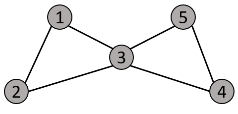
Figure 1: The graph structure of five nodes.

Consider a matrix equation:

$$\mathbf{A}\mathbf{X}+\mathbf{X}\mathbf{B}=\mathbf{C},\mathbf{A},\mathbf{B},\mathbf{C}\in\mathbb{R}^{5\times 5},$$ (12)

where

$$\mathbf{A}=[7\ 1\ 1\ 1\ 5;7\ 2\ 8\ 3\ 0;1\ 4\ 8\ 7\ 7;7\ 8\ 4\ 6\ 7;5\ 8\ 6\ 8\ 5];$$

$$\mathbf{B}=[6\ 6\ 7\ 4\ 4;6\ 0\ 6\ 3\ 4;3\ 2\ 3\ 6\ 5;5\ 0\ 8\ 6\ 6;1\ 1\ 0\ 1\ 6];$$

$$\mathbf{C}=[2\ 4\ 6\ 8\ 7;5\ 8\ 2\ 4\ 2;5\ 3\ 4\ 1\ 7;1\ 5\ 6\ 1\ 2;1\ 2\ 7\ 2\ 7].$$

It can be verified that this equation has a unique solution $\mathbf{X}^{*}$. The related $5$ nodes in an interconnected network forms a graph shown in Fig. 1.

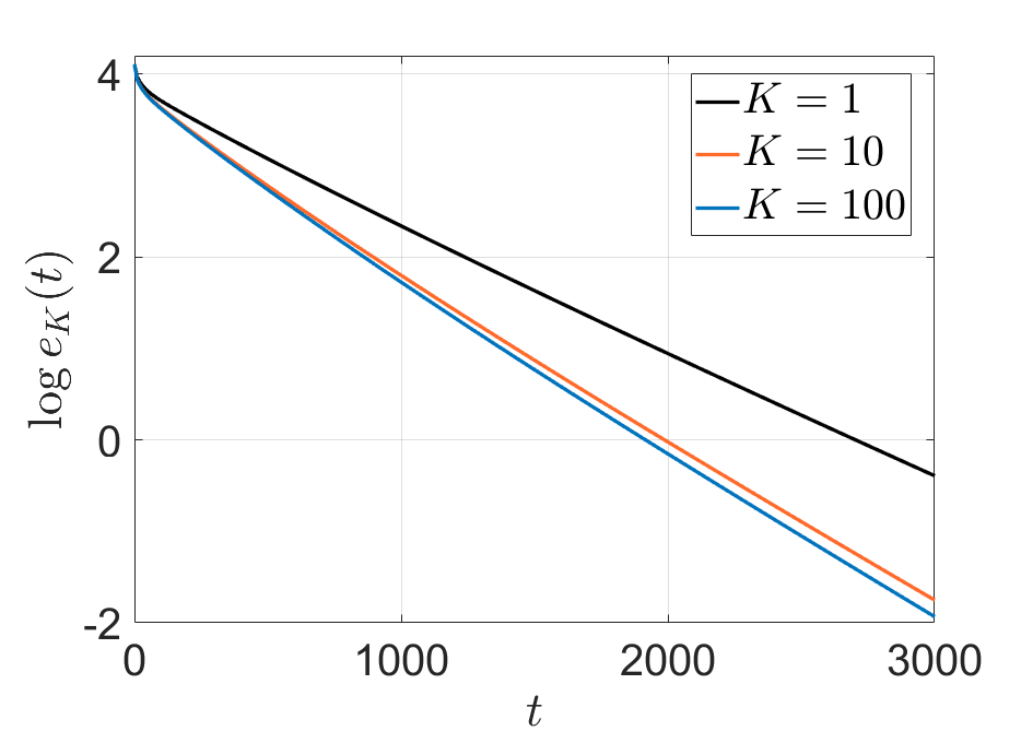
Figure 2: The evolution of $\log e_{K}(t)$ for $K=1,10,100,$ respectively.

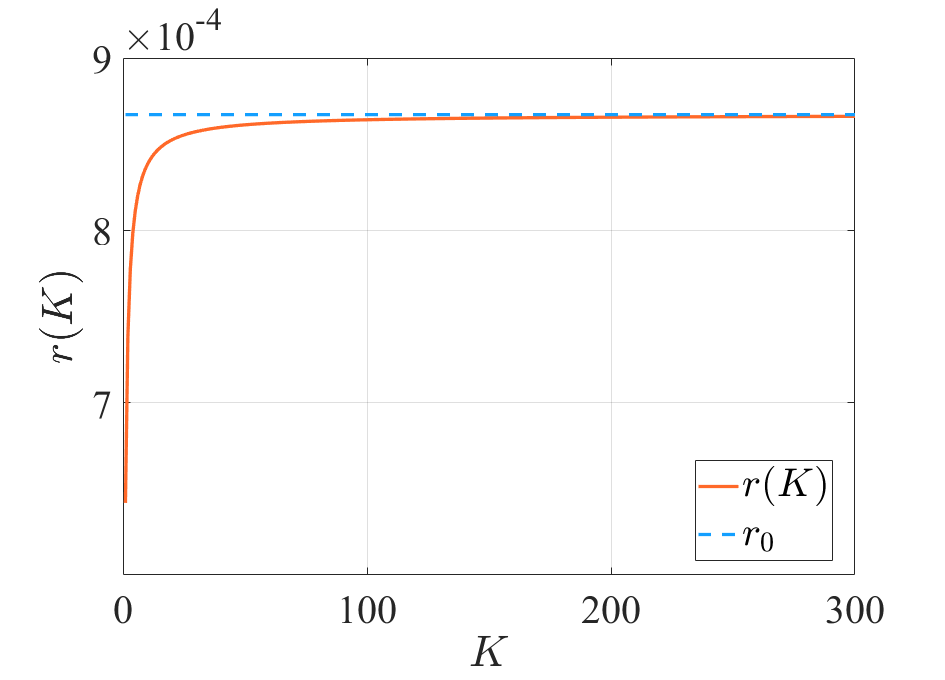
Figure 3: The trajectories of $r(K)$ over $K$ and the reference $r_{0}$.

Taking the initial value to be $\mathbf{0}$, we plot the trajectories of

$$e_{K}(t):=\sum_{i=1}^{5}\|\mathbf{x}_{i}(t)-\mathrm{vec}(\mathbf{X}^{*})\|^{2},$$ (13)

in logarithmic scales for $\mathbf{x}_{i}(t)$ evolving along (8) with $K=1,10,100,$ respectively, in Fig. 2, which validates the exponential convergence in Theorem 1. With different values of $K,$ we calculate $r(K)$ and plot $r(K)$ over $K$ in Fig. 3 with $r_{0}=\lambda_{\mathrm{rank}(\mathbf{H})}((\sum_{i=1}^{n}\mathbf{H}^{{\dagger}}_{i}\mathbf{H}_{i})/n)$ drawn as a reference. Fig. 3 shows that $r(K)$ increases as $K$ increases and $r(K)$ always has an upper bound, which is consistent with $r_{0}=\lim\limits_{K\to\infty}r(K)$.

Example 2. Still consider an equation in the form of (12) and an interconnected network shown in Fig. 1. We investigate two sets of data for $\mathbf{A},\mathbf{B},\mathbf{C}$ as

$$\mathbf{A}^{[1]}=[0\ 0\ 0\ 5\ 0;0\ 2\ 0\ 0\ 2;1\ 3\ 0\ 0\ 0;0\ 0\ 4\ 0\ 0;0\ 0\ 0\ 0\ 0];$$

$$\mathbf{B}^{[1]}=[7\ 4\ 4\ 7\ 10;3\ 8\ 6\ 7\ 3;10\ 8\ 7\ 2\ 6;0\ 2\ 8\ 1\ 2;4\ 5\ 3\ 5\ 8];$$

$$\mathbf{C}^{[1]}=[8\ 1\ 6\ 8\ 3;8\ 5\ 5\ 3\ 7;4\ 8\ 0\ 5\ 7;6\ 9\ 3\ 2\ 7;1\ 1\ 2\ 6\ 5];$$

$$\mathbf{A}^{[2]}=[1\ 5\ 10\ 1\ 9;2\ 10\ 0\ 4\ 2;9\ 1\ 8\ 3\ 3;2\ 4\ 8\ 8\ 1;8\ 1\ 9\ 4\ 1];$$

$$\mathbf{B}^{[2]}=[0\ 0\ 8\ 6\ 0;2\ 0\ 0\ 0\ 0;0\ 1\ 0\ 0\ 0;0\ 0\ 0\ 0\ 0;0\ 0\ 0\ 0\ 3];$$

$$\mathbf{C}^{[2]}=[9\ 6\ 2\ 0\ 3;6\ 4\ 1\ 9\ 9;5\ 5\ 2\ 9\ 4;1\ 4\ 2\ 5\ 1;9\ 1\ 4\ 5\ 8].$$

It can be seen that (i) $\mathbf{A}^{[1]}$ is sparse, $\mathbf{B}^{[1]}$ is dense; (ii) $\mathbf{A}^{[2]}$ is dense, $\mathbf{B}^{[2]}$ is sparse.

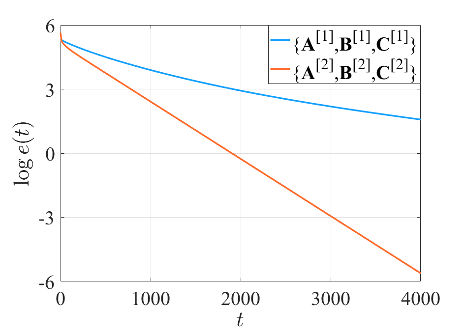
Figure 4: The trajectories of $\log e(t)$ for two problems with data sets $\{\mathbf{A}^{[i]},\mathbf{B}^{[i]},\mathbf{C}^{[i]}\},i=1,2$ under $\mathbf{B}$-$\mathbf{C}$ Column Partition in Example 2.

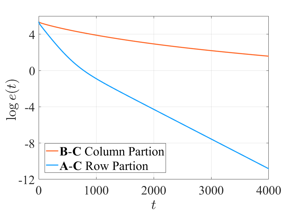
Figure 5: The trajectories of $\log e(t)$ for problem $\{\mathbf{A}^{[1]},\mathbf{B}^{[1]},\mathbf{C}^{[1]}\}$ under partitions $\mathbf{B}$-$\mathbf{C}$ Column and $\mathbf{A}$-$\mathbf{C}$ Row, respectively, in Example 2.

In Fig. 5, we plot the trajectories of $e(t)$ (as setting $K=1$ in (13)) in logarithmic scales under the $\mathbf{B}$-$\mathbf{C}$ Column Partition for the two data sets $\{\mathbf{A}^{[1]},\mathbf{B}^{[1]},\mathbf{C}^{[1]}\}$ and $\{\mathbf{A}^{[2]},\mathbf{B}^{[2]},\mathbf{C}^{[2]}\}$, respectively. It can be seen that faster convergence is achieved at $\{\mathbf{A}^{[2]},\mathbf{B}^{[2]},\mathbf{C}^{[2]}\}$. In Fig. 5, we plot the trajectories of $e(t)$ in logarithmic scales for $\{\mathbf{A}^{[1]},\mathbf{B}^{[1]},\mathbf{C}^{[1]}\}$ under partitions $\mathbf{B}$-$\mathbf{C}$ Column and $\mathbf{A}$-$\mathbf{C}$ Row, respectively. These figures show that the size of data for each node in different partitions has an effect on the convergence rate. Such examples motivate us to advance a conjecture about the existence of data complexity vs. convergence speed tradeoffs for the design of distributed algorithms.

3.5 Discussions

3.5.1 General Sylvester Equation

Consider the Sylvester equation in its general form:

$$\mathbf{A}\mathbf{X}+\mathbf{X}\mathbf{B}=\mathbf{C},\ \mathbf{A}\in\mathbb{R}^{n\times n},\mathbf{B}\in\mathbb{R}^{m\times m},\mathbf{C}\in\mathbb{R}^{n\times m}.$$ (14)

Note that the vectorized form (2) continues to apply to (14). We define a $m$-node ($n$-node) network under the $\mathbf{B}$-$\mathbf{C}$ Column ($\mathbf{A}$-$\mathbf{C}$ Row) Partition. Then the flow (8) can be utilized in the same form, leading to the convergence results under slightly different indices, e.g., under the $\mathbf{B}$-$\mathbf{C}$ Column Partition the limit of rate in Theorem 1 will be read as

$$\lim\limits_{K\to\infty}r(K)=\lambda_{\mathrm{rank}(\mathbf{H})}(\frac{1}{m}(\sum_{i=1}^{m}\mathbf{H}^{{\dagger}}_{i}\mathbf{H}_{i})).$$

3.5.2 Higher-resolution Data Partition

Define a $n^{2}$-node network with node set $\mathrm{V}^{\mathrm{H}}=\{1,2,\cdots,n^{2}\}$ forming a graph $\mathrm{G}^{\mathrm{H}}=(\mathrm{V}^{\mathrm{H}},\mathrm{E}^{\mathrm{H}}).$ Suppose that the index of node $i$ satisfies $i=(k-1)n+l$ with $k=1,\cdots,n,l=1,\cdots,n.$ Then any $i\in\mathrm{V}^{\mathrm{H}}$ can be uniquely represented by a binary array $(k,l).$ Here we have the partition that node $i(k,l)$ holds the $l$-th row of $\mathbf{A}$, the $k$-th column of $\mathbf{B}$ and the $(l,k)$-th entry of $\mathbf{C}$, denoted by $(\mathbf{A}^{T})_{l}^{T},B_{k}$ and $\mathbf{C}_{lk}$. Denote

$$[\mathbf{A}_{0}]_{i(k,l)}:=e_{k}^{T}\otimes(\mathbf{A}^{T})_{l}^{T},\quad[\mathbf{B}_{e}]_{i(k,l)}:=e_{l}^{T}(\mathbf{B}_{k}^{T}\otimes\mathbf{I}_{n}).$$

Then node $i(k,l)$ has access to the equation $\big{(}[\mathbf{A}_{0}]_{i(k,l)}+[\mathbf{B}_{e}]_{i(k,l)}\big{)}\mathrm{vec}(\mathbf{X})=\mathbf{C}_{lk}.$ For $i(k,l)=i\in\mathrm{V}^{\mathrm{H}}$, denote

$$\mathcal{E}^{\mathrm{H}}_{i(k,l)}:=\{\mathbf{y}\in\mathbb{R}^{n^{2}}:\Big{(}[\mathbf{A}_{0}]_{i(k,l)}+[\mathbf{B}_{e}]_{i(k,l)}\Big{)}\mathbf{y}=\mathbf{C}_{lk}\}.$$

Case (I) and Case (II) guarantee that $\mathcal{E}^{\mathrm{H}}_{i(k,l)}$ and their intersection are nonempty. Therefore, our preceding discussion can be easily applied to this partition with designing the flow

$$\dot{\mathbf{x}}_{i}=K(\sum_{j\in\mathrm{N}_{i}}(\mathbf{x}_{j}-\mathbf{x}_{i}))+\mathcal{P}_{\mathcal{E}^{\mathrm{H}}_{i(k,l)}}(\mathbf{x}_{i})-\mathbf{x}_{i},\quad i\in\mathrm{V}^{\mathrm{H}}.$$

With $\mathcal{E}^{\mathrm{H}}:=\cap_{i=1}^{n}\mathcal{E}^{\mathrm{H}}_{i(k,l)}$ and

$$\mathbf{h}_{i}:=[\mathbf{A}_{0}]_{i(k,l)}+[\mathbf{B}_{e}]_{i(k,l)}\in\mathbb{R}^{1\times n^{2}}$$

$(\mathbf{h}_{i}^{{\dagger}}\mathbf{h}_{i}=\frac{\mathbf{h}_{i}^{T}\mathbf{h}_{i}}{\mathbf{h}_{i}\mathbf{h}_{i}^{T}}$ if $\mathbf{h}_{i}\neq\mathbf{0},\mathbf{h}_{i}^{{\dagger}}\mathbf{h}_{i}=\mathbf{0}$ otherwise), we have

$$\lim\limits_{t\to\infty}\mathbf{x}_{i}(t)=\sum_{i=1}^{n^{2}}\mathcal{P}_{\mathcal{E}^{\mathrm{H}}}(\mathbf{x}_{i}(0))/n^{2},\quad\forall i\in\mathrm{V}^{\mathrm{H}}.$$

The rate of exponential convergence $\tilde{r}(K)$ satisfies that

$$\lim\limits_{K\to\infty}\tilde{r}(K)=\lambda_{\mathrm{rank}(\mathbf{H})}(\frac{1}{n^{2}}(\sum_{i=1}^{n^{2}}\mathbf{h}^{{\dagger}}_{i}\mathbf{h}_{i})).$$

Compared with the case for an $n$-node network, in which each node holds $n^{2}+2n$ scalar elements of data, each node only needs to hold $2n+1$ scalar elements of data in the higher-resolution data partition case for an $n^{2}$-node network.

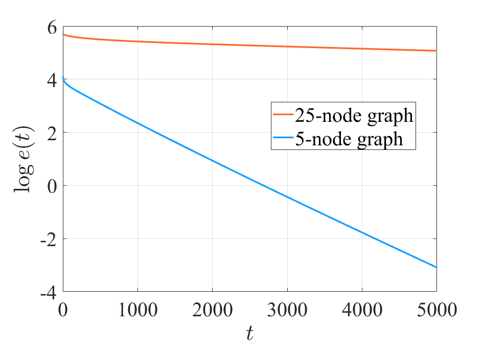
Figure 6: The trajectories of $\log e(t)$ for two networks with cycle graph and $K=1$ in Example 3.

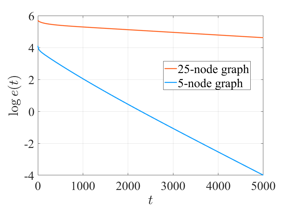
Figure 7: The trajectories of $\log e(t)$ for two networks with complete graph and $K=1$ in Example 3.

Example 3. Consider the same matrix equation as in Example 1. Setting $K=1$ in (13), we plot the trajectories of $\log e(t)$ in Figs. 7 and 7, where we adopt cyclic graphs and complete graphs with $5$ and $25$ nodes, respectively. Each node in the $5$-node network holds the data with the size of $(5^{2}+2\times 5)$, while each node in the $25$-node network holds $(2\times 5+1)$. Though the data complexity does decrease for every node in the $25$-node network, the convergence rate of the $5$-node network is much faster. This indicates the existence of data distribution vs. convergence speed tradeoffs for the design of distributed algorithms.

3.5.3 Lyapunov Equations

When $\mathbf{B}=\mathbf{A}^{T},$ we consider a Lyapunov equation with respect to variable $\mathbf{X}\in\mathbb{R}^{n\times n}$:

$$\mathbf{A}\mathbf{X}+\mathbf{X}\mathbf{A}^{T}=\mathbf{C},\quad\mathbf{A},\mathbf{C}\in\mathbb{R}^{n\times n},$$ (15)

where $\mathbf{C}$ is a symmetric matrix. If $\mathbf{X}_{0}$ is the unique solution to (15), it must hold that $\mathbf{X}_{0}=\mathbf{X}_{0}^{T}.$ If $\mathbf{X}_{0}$ is a solution to (15) when there exist an infinite number of solutions, it must hold that $\mathbf{X}_{0}^{T}$ is also a solution to (15). Due to the symmetry of $\mathbf{C}$, under the higher-resolution data partition in 3.5.2, we can alternatively adopt a network $\hat{\mathrm{G}}=(\hat{\mathrm{V}},\hat{\mathrm{E}})$ with $n(n+1)/2$ nodes rather than $n^{2}$ nodes. The node $i$ is assigned with the data set

$$\mathcal{F}_{i}:=\big{\{} \big{(}(\mathbf{A}^{T})_{l}^{T},(\mathbf{A}^{T})_{k}^{T},\mathbf{C}_{lk},\mathbf{C}_{kl}\big{)}:k\leq l,k,l\in\{1,\cdots,n\}i=g(k,l)=(k-1)n+l-k(k-1)/2\big{\}}.$$

Defining $f(k,l)=(k-1)n+l$, we introduce the affine subspaces

$$\hat{\mathcal{E}}_{i}:=\Big{\{} \mathbf{y}\in\mathbb{R}^{n^{2}}:\hat{\mathbf{H}}_{i}\mathbf{y}=\mathrm{col}\{\mathbf{C}_{lk},\mathbf{C}_{kl}\},\hat{\mathbf{H}}_{i}=\begin{bmatrix}[\mathbf{A}_{0}]_{f(k,l)}+[\mathbf{A}^{T}_{e}]_{f(k,l)}\\ [\mathbf{A}_{0}]_{f(l,k)}+[\mathbf{A}^{T}_{e}]_{f(l,k)}\end{bmatrix},$$

$$i=g(k,l),k\leq l,k,l\in\{1,\cdots,n\}\Big{\}},\quad i\in\hat{\mathrm{V}},$$

where $[\mathbf{A}_{0}]_{f(k,l)}:=e_{k}^{T}\otimes(\mathbf{A}^{T})_{l}^{T}$ and $[\mathbf{A}^{T}_{e}]_{f(k,l)}:=e_{l}^{T}(\mathbf{A}_{k}\otimes\mathbf{I}_{n})$. We can modify the flow (8) to

$$\dot{\mathbf{x}}_{i}=K(\sum_{j\in\mathrm{N}_{i}}(\mathbf{x}_{j}-\mathbf{x}_{i}))+\mathcal{P}_{\hat{\mathcal{E}}_{i}}(\mathbf{x}_{i})-\mathbf{x}_{i},\quad i\in\hat{\mathrm{V}}.$$ (16)

Based on the same analysis, along (16) $\mathrm{vec}^{-1}(\mathbf{x}_{i}(t))$ continues to converge to a solution of (15), with the rate of exponential convergence described by $\hat{r}(K)$, and

$$\lim\limits_{K\to\infty}\hat{r}(K)=\lambda_{\mathrm{rank}(\mathbf{H})}(\frac{1}{n(n+1)/2}(\sum_{i=1}^{n(n+1)/2}\hat{\mathbf{H}}^{{\dagger}}_{i}\hat{\mathbf{H}}_{i})).$$

4 Full Row/Column Partition

In this section, we investigate the full partitions of the data matrices $\mathbf{A}$, $\mathbf{B}$ and $\mathbf{C}$ along rows and columns, and present effective flows to solve the equation (1) under such partitions over an $n$-node network.

4.1 Full Row/Column Partition

We consider two full partitions of the $(\mathbf{A},\mathbf{B},\mathbf{C})$-triplet.

• $[\mathbf{A}$ Row/$\mathbf{B}$-$\mathbf{C}$ Column Partition$]$ Node $i$ holds the $i$-th row of $\mathbf{A}$, and the $i$-th column of $\mathbf{B}$ and $\mathbf{C}$, denoted by $(\mathbf{A}^{T})_{i}^{T},\mathbf{B}_{i}$ and $\mathbf{C}_{i}$, respectively.

• [$\mathbf{A}$-$\mathbf{C}$ Row/$\mathbf{B}$ Column Partition] Node $i$ holds the $i$-th row of $\mathbf{A}$ and $\mathbf{C}$, and the $i$-th column of $\mathbf{B}$, denoted by $(\mathbf{A}^{T})_{i}^{T},(\mathbf{C}^{T})_{i}^{T}$ and $\mathbf{B}_{i}$, respectively.

These two partitions are equivalent in the sense of $\mathbf{A}\mathbf{X}+\mathbf{X}\mathbf{B}=\mathbf{C}$ and $\mathbf{B}^{T}\mathbf{X}^{T}+\mathbf{X}^{T}\mathbf{A}^{T}=\mathbf{C}^{T}.$ Thus, we focus on the $\mathbf{A}$ Row/$\mathbf{B}$-$\mathbf{C}$ Column Partition in our analysis.

Remark 5.

There may be other full row/column partitions, obtained e.g. through partitioning $\mathbf{A},\mathbf{B}$ by row and $\mathbf{C}$ by column or partitioning $\mathbf{A},\mathbf{B},\mathbf{C}$ by column. By using appropriate equivalence transformation, we can deal with these partitions in a similar way, so more specific details are omitted.

4.2 An Augmented “Consensus $+$ Projection” Flow

For $i\in\mathrm{V}$, define

$$\mathcal{E}_{i}^{\text{Aug}}=\{\mathbf{y}=\mathrm{vec}([\mathbf{X},\mathbf{Z}])\in\mathbb{R}^{n^{2}(1+n)}:\mathbf{e}_{i}(\mathbf{A}^{T})_{i}^{T}\mathbf{X}+\mathbf{X}\mathbf{B}_{i}\mathbf{e}_{i}^{T}-(({\mathbf{L}_{\mathrm{G}}^{T}})_{i}^{T}\otimes\mathbf{I}_{n})\mathbf{Z}=\mathbf{C}_{i}\mathbf{e}_{i}^{T}\},$$ (17)

and a projection mapping $\mathcal{P}_{\mathcal{E}_{i}^{\text{Aug}}}:\mathbb{R}^{n^{2}(1+n)}\to\mathcal{E}_{i}^{\text{Aug}}$. We propose the following augmented network flow for $\mathbf{y}_{i}(t)=\mathrm{col}\{\mathbf{x}_{i}(t),\mathbf{z}_{i}(t)\}$ with $\mathbf{x}_{i}(t)\in\mathbb{R}^{n^{2}}$,

$$\dot{\mathbf{y}}_{i}=K\Big{(}\sum_{j\in\mathrm{N}_{i}}(\mathbf{y}_{j}-\mathbf{y}_{i})\Big{)}+\mathcal{P}_{\mathcal{E}_{i}^{\text{Aug}}}(\mathbf{y}_{i})-\mathbf{y}_{i},\quad i\in\mathrm{V},$$ (18)

where $\mathbf{y}_{i}\in\mathbb{R}^{n^{2}(1+n)}$, and $\mathrm{vec}^{-1}(\mathbf{x}_{i})\in\mathbb{R}^{n\times n}$ is what we are interested in.

Theorem 3.

Under the $\mathbf{A}$ Row/$\mathbf{B}$-$\mathbf{C}$ Column Partition, for any initial value $\mathbf{y}_{0}=\mathrm{col}\{\mathbf{y}_{1}(0),\cdots,\mathbf{y}_{n}(0)\}$, there exists $\mathbf{X}^{*}(\mathbf{y}_{0})\in\mathbb{R}^{n\times n}$ as a solution to (1), such that $\mathrm{vec}^{-1}(\mathbf{x}_{i}(t))=\mathrm{vec}^{-1}([\mathbf{I}_{n^{2}},\mathbf{0}_{n^{2}\times n^{3}}]\mathbf{y}_{i}(t))$ along the flow (18) converges to $\mathbf{X}^{*}(\mathbf{y}_{0})$ exponentially, for all $i\in\mathrm{V}$.

The proof of Theorem 3 is given in Appendix D.

4.3 Application for the Motivating Example

The network flow (18) can be used to solve the problem arising from the motivating example mentioned in subsection 2.2. Each node $i$ representing subsystem $i$ only knows the information $\mathbf{D}_{ij}\in\mathbb{R}^{m\times m},j\in\mathrm{V}$ and communicates with its neighbors for exchanging state information. We utilize the flow (18) via substituting

$$(\mathbf{A}^{T})_{i}^{T}=[\mathbf{D}_{i1},\cdots\mathbf{D}_{in}],\ \mathbf{B}_{i}=\mathrm{col}\{\mathbf{D}_{i1},\cdots\mathbf{D}_{in}\},\ \mathbf{C}_{i}=-(\mathbf{I}_{mn})_{i},$$

into $\mathcal{E}_{i}^{\text{Aug}}$ in (17). As a result, along the flow (18) carried out over $\mathrm{G}$, node $i$ can obtain an evolutionary state $\mathrm{vec}^{-1}(\mathbf{x}_{i}(t))$ by communicating and computing. Then every node can draw a conclusion about the stability of the overall network after confirming two conditions:

• Each $\mathrm{vec}^{-1}(\mathbf{x}_{i}(t))$ converges to a positive definite matrix at node $i$;

• All $\mathrm{vec}^{-1}(\mathbf{x}_{i}(t))$ converge to the same limit.

It is easy to see while condition (i) can be verified by each node $i$ by itself, and condition (ii) can be established distributedly by for example, running a consensus algorithm for the node state limits.

Example 4. Consider three subsystems $i=1,2,3$, in the dynamics is in the form of (3) with

$$\mathbf{D}_{11} =\begin{bmatrix}-5&0\\ 0&-5\end{bmatrix},\ \mathbf{D}_{12}=\begin{bmatrix}4&1\\ 0&4\end{bmatrix},\ \mathbf{D}_{13}=\mathbf{0}_{2\times 2},$$

$$\mathbf{D}_{21} =\begin{bmatrix}1&0\\ 0&1\end{bmatrix},\ \mathbf{D}_{22}=\begin{bmatrix}-6&1\\ 1&-3\end{bmatrix},\ \mathbf{D}_{23}=\begin{bmatrix}2&0\\ 2&4\end{bmatrix},$$

$$\mathbf{D}_{31} =\mathbf{0}_{2\times 2},\ \mathbf{D}_{32}=\begin{bmatrix}2&0\\ 1&-1\end{bmatrix},\ \mathbf{D}_{33}=\begin{bmatrix}-4&0\\ 0&-4\end{bmatrix}.$$

The network communication structure is shown as Fig. 8, whose Laplacian matrix is

$$\mathbf{L}_{\mathrm{G}}=[1,-1,0;-1,2,-1;0,-1,1].$$

Figure 8: The communicate graph in Example 4.

Each node $i$ can compute $\mathcal{P}_{\mathcal{E}_{i}^{\text{Aug}}}(\cdot)$ in (17) according to Lemma 5. Under the network flow (18), there holds

$$\lim\limits_{t\to\infty}\mathrm{vec}^{-1}(\mathbf{x}_{i}(t))=\mathbf{P}^{*}=\begin{bmatrix}0.2278&0.1343&0.1176&0.1690&0.0744&-0.0009\\ 0.1343&0.3170&0.0990&0.2713&0.0694&-0.0068\\ 0.1176&0.0990&0.1529&0.1360&0.0819&0.0040\\ 0.1690&0.2713&0.1360&0.4106&0.1067&0.0278\\ 0.0744&0.0694&0.0819&0.1069&0.1660&-0.0021\\ -0.0009&-0.0068&0.0040&0.0278&-0.0021&0.1190\end{bmatrix},$$

where $\mathbf{P}^{*}$ is a positive definite solution to

$$\mathbf{A}\mathbf{X}+\mathbf{X}\mathbf{A}^{T}=-\mathbf{I}_{6}$$

with $\mathbf{A}=[\mathbf{D}_{11},\mathbf{D}_{12},\mathbf{D}_{13};\mathbf{D}_{21},\mathbf{D}_{22},\mathbf{D}_{23};\mathbf{D}_{31},\mathbf{D}_{32},\mathbf{D}_{33}].$ See from Fig. 9 the trajectory of

$$e(t)=\frac{1}{3}\sum_{i=1}^{3}\|\mathrm{vec}^{-1}(\mathbf{x}_{i}(t))-\mathbf{P}^{*}\|_{F}^{2}$$

in logarithmic scales.

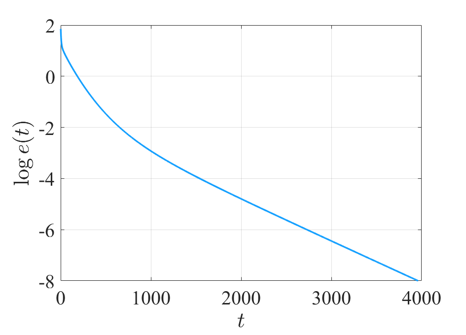
Figure 9: The trajectories of $e(t)$ in Example 4.

As for every subsystem, on the one hand, it can hold the information that $\mathrm{vec}^{-1}(\mathbf{x}_{i}(t))$ converges to a positive definite matrix $\mathbf{P}^{*}$. On the other hand, they can carry out a consensus test and have confirmed that all the subsystems states along (18) are reaching a consensus state. Then every subsystem can conclude that the whole system is stable, which is in agreement with the fact that the global matrix $\mathbf{A}$ is Hurwitz.

5 Clustering Block Partition

In this section, we turn to clustering block partitions of $\mathbf{A},\mathbf{B},\mathbf{C}$ for seeking distributed solutions of the equation (1). It seems possible that, for certain structured matrices, general block partitions may be particularly useful.

5.1 Clustering Block Partition

Consider a double-layer network that has $n$ clusters with each cluster having $n$ nodes. These clusters are indexed in $\mathrm{V}=\{1,\cdots,n\}$ forming an outer layer graph $\mathrm{G}=(\mathrm{V},\mathrm{E}),$ while the nodes in cluster $i$ are indexed in $\mathrm{V}_{i}=\{i_{1},\cdots,i_{n}\}$ forming an inner layer graph $\mathrm{G}_{i}=(\mathrm{V}_{i},\mathrm{E}_{i}).$ In total there are $n^{2}$ nodes in the overall network. The neighbor set of cluster $i$ is given by $\mathrm{N}_{i}:=\{j:(i,j)\in\mathrm{E}\}$, which means that nodes in cluster $i$ can receive information from nodes in its neighbor clusters; meanwhile, the neighbor set of node $i_{j}$ in cluster $i$ is given by $\mathrm{N}_{i_{j}}:=\{i_{k}:(i_{j},i_{k})\in\mathrm{E}_{i}\}$, which means that node $i_{j}$ can receive information from its neighbor nodes in its own cluster. Let $\mathbf{L}_{\mathrm{G}}$ and $\mathbf{L}_{\mathrm{G}_{i}}$ denote the Laplacian matrix of the outer layer graph (linking the clusters) and inner layer graphs (linking nodes in each cluster), respectively. We recall $\mathbf{H}=\mathbf{I}_{n}\otimes\mathbf{A}+\mathbf{B}^{T}\otimes\mathbf{I}_{n}$ and define the $i$-th column of $\mathbf{C}$ as $\mathbf{C}_{i}=\sum\nolimits_{j=1}^{n}\mathbf{C}_{ji}\mathbf{e}_{j}$ with $\mathbf{C}_{ji}$ being the $(j,i)$-th entry of $\mathbf{C}$. Define an indicator function $\mathbf{1}_{\{j=i\}}$, where $\mathbf{1}_{\{j=i\}}=1$ if $j=i,$ and $\mathbf{1}_{\{j=i\}}=0,$ otherwise. Then we consider the following data partition.

[Column $\mathbf{B}$-$\mathbf{C}$ Block Partition, as in Table 1] The node $i_{j}$ holds $\mathbf{B}_{ji}$ and $\mathbf{C}_{ji}$ (the $(j,i)$-th entry of $\mathbf{B}$ and $\mathbf{C}$), and additionally, the node $i_{i}$ holds $\mathbf{A}$. Together, we say cluster $i$ holds $\mathbf{A},$ $\mathbf{B}_{i}$ and $\mathbf{C}_{i}$. Specifically, each node $i_{j}$ holds a state $\mathbf{x}_{i_{j}}\in\mathbb{R}^{n}$, while the cluster state $\mathbf{x}_{i}=\mathrm{col}\{\mathbf{x}_{i_{1}},\cdots,\mathbf{x}_{i_{n}}\}\in\mathbb{R}^{n^{2}}$ satisfies

$$\sum\limits_{j=1}^{n}\left((\mathbf{1}_{\{j=i\}}\mathbf{A}+\mathbf{B}_{ji}\mathbf{I}_{n})\mathbf{x}_{i_{j}}-\mathbf{C}_{ji}\mathbf{e}_{j}\right)=\mathbf{0}_{n}.$$

Table 1: The Column $\mathbf{B}$-$\mathbf{C}$ Block Partition.

	$1$-st Node	$2$-nd Node	$\cdots$	$n$-th Node
Cluster 1	$\mathbf{A},\mathbf{B}_{11},\mathbf{C}_{11}$	$\mathbf{B}_{21},\mathbf{C}_{21}$	$\cdots$	$\mathbf{B}_{n1},\mathbf{C}_{n1}$
Cluster 2	$\mathbf{B}_{12},\mathbf{C}_{12}$	$\mathbf{A},\mathbf{B}_{22},\mathbf{C}_{22}$	$\cdots$	$\mathbf{B}_{n2},\mathbf{C}_{n2}$
$\vdots$	$\vdots$	$\vdots$	$\ddots$	$\vdots$
Cluster n	$\mathbf{B}_{1n},\mathbf{C}_{1n}$	$\mathbf{B}_{2n},\mathbf{C}_{2n}$	$\cdots$	$\mathbf{A},\mathbf{B}_{nn},\mathbf{C}_{nn}$

Therefore, all the estimates from clusters need to reach a consensus $\mathbf{x}_{1}^{*}=\cdots=\mathbf{x}_{n}^{*}$, which is the estimation of a solution to (2). In view of [13], essentially any data block partition would work if the algorithm can be correspondingly designed.

5.2 “Local Conservation + Global Consensus” Flow

Take an auxiliary variable $\mathbf{z}_{i_{j}}\in\mathbb{R}^{n}$ associated with and known by node $i_{j}.$ Each node $i_{j}$ can obtain the information about $\mathbf{z}_{i_{k}},i_{k}\in\mathrm{N}_{i_{j}}$ from its neighbors within the same cluster. Then the auxiliary variables of all nodes within the cluster $i$ combine the cluster variable $\mathbf{z}_{i}=\mathrm{col}\{\mathbf{z}_{i_{1}},\cdots,\mathbf{z}_{i_{n}}\}\in\mathbb{R}^{n^{2}}$. Each node $i_{j}$ holds state $\mathbf{x}_{i_{j}}\in\mathbb{R}^{n}$ and gets the information about $\mathbf{x}_{k_{j}},k\in\mathrm{N}_{i}$ from its neighbor clusters and then the states of all nodes within the cluster $i$ combine the cluster state $\mathbf{x}_{i}=\mathrm{col}\{\mathbf{x}_{i_{1}},\cdots,\mathbf{x}_{i_{n}}\}\in\mathbb{R}^{n^{2}}$. Let $K>0$ be a given constant. We propose the following continuous-time network flow:

$$\dot{\mathbf{x}}_{i_{j}}= -(\mathbf{1}_{\{j=i\}}\mathbf{A}+\mathbf{B}_{ji}\mathbf{I}_{n})^{T}((\mathbf{1}_{\{j=i\}}\mathbf{A}+\mathbf{B}_{ji}\mathbf{I}_{n})\mathbf{x}_{i_{j}}-\mathbf{C}_{ji}\mathbf{e}_{j}-\sum_{i_{k}\in\mathrm{N}_{i_{j}}}(\mathbf{z}_{i_{j}}-\mathbf{z}_{i_{k}}))-K\sum_{k\in\mathrm{N}_{i}}(\mathbf{x}_{i_{j}}-\mathbf{x}_{k_{j}}),$$ (19)

$$\dot{\mathbf{z}}_{i_{j}}= (\mathbf{1}_{\{j=i\}}\mathbf{A}+\mathbf{B}_{ji}\mathbf{I}_{n})\mathbf{x}_{i_{j}}-\mathbf{C}_{ji}\mathbf{e}_{j}-\sum_{i_{k}\in\mathrm{N}_{i_{j}}}(\mathbf{z}_{i_{j}}-\mathbf{z}_{i_{k}}).$$

Denote $\mathbf{M}_{i}=\mathrm{diag}\{\mathbf{1}_{\{j=i\}}\mathbf{A}+\mathbf{B}_{ji}\mathbf{I}_{n},j=1,\cdots,n\}$ and $\tilde{\mathbf{C}}_{i}=\mathrm{col}\{\mathbf{C}_{1i}\mathbf{e}_{1},\cdots,\mathbf{C}_{ni}\mathbf{e}_{n}\}$; then we reformulate (19) as

$$\dot{\mathbf{x}}_{i}= -\mathbf{M}_{i}^{T}(\mathbf{M}_{i}\mathbf{x}_{i}-\tilde{\mathbf{C}}_{i}-(\mathbf{L}_{\mathrm{G}_{i}}\otimes\mathbf{I}_{n})\mathbf{z}_{i})-K\sum_{k\in\mathrm{N}_{i}}(\mathbf{x}_{i}-\mathbf{x}_{k}),$$ (20)

$$\dot{\mathbf{z}}_{i}= \mathbf{M}_{i}\mathbf{x}_{i}-\tilde{\mathbf{C}}_{i}-(\mathbf{L}_{\mathrm{G}_{i}}\otimes\mathbf{I}_{n})\mathbf{z}_{i}.$$

We further define $\bar{\mathbf{M}}=\mathrm{diag}\{\mathbf{M}_{i},i=1,\cdots,n\}$, $\bar{\mathbf{C}}=\mathrm{col}\{\tilde{\mathbf{C}}_{i},\cdots,\tilde{\mathbf{C}}_{n}\}$, $\bar{\mathbf{L}}=\mathrm{diag}\{\mathbf{L}_{\mathrm{G}_{i}}\otimes\mathbf{I}_{n},i=1,\cdots,n\}$ and $\mathbf{z}=\mathrm{col}\{\mathbf{z}_{1},\cdots,\mathbf{z}_{n}\},\mathbf{x}=\mathrm{col}\{\mathbf{x}_{1},\cdots,\mathbf{x}_{n}\}$. The flow (20) can be rewritten as a compact form

$$\dot{\mathbf{x}} =-\bar{\mathbf{M}}^{T}(\bar{\mathbf{M}}\mathbf{x}-\bar{\mathbf{C}}-\bar{\mathbf{L}}\mathbf{z})-K(\mathbf{L}_{\mathrm{G}}\otimes\mathbf{I}_{n^{2}})\mathbf{x},$$ (21)

$$\dot{\mathbf{z}} =\bar{\mathbf{M}}\mathbf{x}-\bar{\mathbf{C}}-\bar{\mathbf{L}}\mathbf{z}.$$

Denoting $\mathbf{G}:=\begin{bmatrix}\bar{\mathbf{M}}^{T}\bar{\mathbf{M}}+K(\mathbf{L}_{\mathrm{G}}\otimes\mathbf{I}_{n^{2}})&-\bar{\mathbf{M}}^{T}\bar{\mathbf{L}}\\ -\bar{\mathbf{M}}&\bar{\mathbf{L}}\end{bmatrix}$, we present the following theorem.

Theorem 4.

Under the Clustering Block Partition, for any initial values $\mathbf{x}_{0}=\mathrm{col}\{\mathbf{x}_{1}(0),\cdots,\mathbf{x}_{n}(0)\},$ and $\mathbf{z}_{0}=\mathrm{col}\{\mathbf{z}_{1}(0),\cdots,\mathbf{z}_{n}(0)\}$, there exists $\mathbf{X}^{*}(\mathbf{x}_{0},\mathbf{z}_{0})\in\mathbb{R}^{n\times n}$ as a solution to (1), such that $\mathrm{vec}^{-1}(\mathbf{x}_{i}(t))$ along the flow (19) converges to $\mathbf{X}^{*}(\mathbf{x}_{0},\mathbf{z}_{0}).$ Moreover, there exist $\beta(\mathbf{x}_{0},\mathbf{z}_{0}),r^{*}(K)>0$, such that for all $t\geq 0,$

$$\sum_{i=1}^{n}\|\mathrm{vec}^{-1}(\mathbf{x}_{i}(t))-\mathbf{X}^{*}(\mathbf{x}_{0},\mathbf{z}_{0})\|_{F}^{2}\leq\beta(\mathbf{x}_{0},\mathbf{z}_{0})e^{-2r^{*}(K)t},$$

where the rate of exponential convergence $r^{*}(K)$ is a non-decreasing function with respect to $K$ satisfying $r^{*}(K)=\lambda_{k}(\mathbf{G})$, where $k=\mathrm{rank}(\mathbf{G})\leq 2n^{3}-n^{2}-\dim(\cap_{i=1}^{n}\ker(\mathbf{M}_{i}))$.

The proof of Theorem 4 is shown in Appendix E.

5.3 Numerical Example

Example 5. Consider the same matrix equation as in Example 1, which has a unique solution. We use the two kinds of networks with a 25-node graph in subsection 3.5.2 and a graph of five 5-node clusters in subsection 5.1, respectively. Define the error function under the Column $\mathbf{B}$-$\mathbf{C}$ Block Partition:

$$E_{K}^{d}(t) =\sum_{i=1}^{5}\|\mathbf{x}_{i}(t)-\mathrm{vec}(\mathbf{X}^{*})\|^{2}=\sum_{i=1}^{5}\|\mathrm{col}\{\mathbf{x}_{i_{1}},\cdots,\mathbf{x}_{i_{5}}\}-\mathrm{vec}(\mathbf{X}^{*})\|^{2}.$$

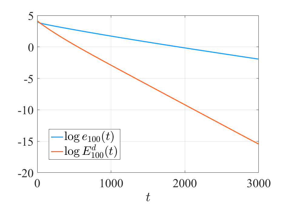
Figure 10: The trajectories of $\log E_{100}^{d}(t)$ and $e_{100}(t)$, respectively.

For a complete graph, taking the zero matrix as the initial value, we plot in Fig. 10 the trajectories of $E_{100}^{d}(t)$ and $e_{100}(t)$ defined in (13) in logarithmic scales for $\mathbf{x}_{i_{j}}(t)$ evolving along (19) and $\mathbf{x}_{i}(t)$ along (8), respectively. Fig. 10 shows that $\mathbf{x}_{i_{j}}(t)$ along the flow (19) converges exponentially and the convergence rate of clustering block partition is much faster than that of partial $\mathbf{B}$-$\mathbf{C}$ Column Partition in Section 3. With different values of $K,$ we can also calculate $r^{*}(K)$ and plot the trajectory of $r^{*}(K)$ over $K$ in Fig. 11, which shows that the rate of exponential convergence is a non-decreasing function with respect to $K$. Results in these figures are consistent with Theorem 4.

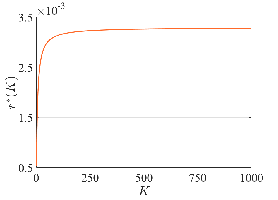
Figure 11: The trajectory of $r^{*}(K)$ over the parameter $K$.

6 Conclusion

This paper has focused on the distributed computation of the multi-agent network for Sylvester matrix equations. We have proposed several network flows for partitions of partial row/column, full row/column and clustering block about the data matrices, inspired by the computation for linear algebraic equations. We have remarked on a special case for symmetric solutions and discussed the general Sylvester equation and others with examples. Accordingly, appropriate partitions could be selected based on actual conditions. The convergence and the limitation of convergence rate have been established in view of matrix theory and linear system theory, which also have been verified by typical numerical examples. Future work includes characterizing the performance of the proposed solutions for general directed and switching networks, as well as methods for accelerating the flows by optimizing network structures.

Appendices

Appendix A Preliminaries

In this appendix, we present some preliminaries on matrix analysis, affine spaces, and exponential stability of dynamical systems.

For a matrix $\mathbf{A}\in\mathbb{R}^{n\times m},$ a M-P pseudoinverse [31] of $\mathbf{A}$ is defined as a matrix $\mathbf{A}^{{\dagger}}\in\mathbb{R}^{m\times n}$ satisfying all of the following four equalities: $(i)\mathbf{A}\mathbf{A}^{{\dagger}}\mathbf{A}=\mathbf{A};(ii)\mathbf{A}^{{\dagger}}\mathbf{A}\mathbf{A}^{{\dagger}}=\mathbf{A}^{{\dagger}};(iii)(\mathbf{A}\mathbf{A}^{{\dagger}})^{T}=\mathbf{A}^{{\dagger}}\mathbf{A};(iv)(\mathbf{A}^{{\dagger}}\mathbf{A})^{T}=\mathbf{A}^{{\dagger}}\mathbf{A}.$ Then the following lemma about the pseudoinverse holds, as well as a lemma about the inequalities of eigenvalues.

Lemma 1 ([16]).

For any matrix $\mathbf{A}\in\mathbb{R}^{n\times m},$ the following statements hold.

1. The M-P pseudoinverse of matrix $\mathbf{A}$ is unique. The pseudoinverse of the pseudoinverse is the original matrix: $(\mathbf{A}^{{\dagger}})^{{\dagger}}=\mathbf{A};$

2. $\mathrm{rank}(\mathbf{A}^{{\dagger}})=\mathrm{rank}(\mathbf{A})=\mathrm{rank}(\mathbf{A}^{T})=\mathrm{rank}(\mathbf{A}^{{\dagger}}\mathbf{A})=\mathrm{rank}(\mathbf{A}\mathbf{A}^{{\dagger}});$

3. $\ker(\mathbf{A}^{{\dagger}})=\ker(\mathbf{A}^{T}),$ $\ker(\mathbf{A})=\ker(\mathbf{A}^{{\dagger}}\mathbf{A});$

4. $(\mathbf{A}^{{\dagger}}\mathbf{A})^{2}=\mathbf{A}^{{\dagger}}\mathbf{A}=(\mathbf{A}^{{\dagger}}\mathbf{A})^{T},$ $\mathbf{A}^{{\dagger}}\mathbf{A}$ is real symmetric and idempotent, and its eigenvalues can only be zero or one.

Lemma 2 (Weyl’s inequality [32]).

Suppose that $\mathbf{M}$ and $\mathbf{N}$ are $n\times n$ symmetric matrices. Then

$$\lambda_{j}(\mathbf{M})+\lambda_{n}(\mathbf{N})\leq\lambda_{j}(\mathbf{M}+\mathbf{N})\leq\lambda_{j}(\mathbf{M})+\lambda_{1}(\mathbf{N}).$$ (22)

Next, for a non-defective matrix, the following lemma holds, where a matrix $\mathbf{M}\in\mathbb{R}^{n\times n}$ is non-defective if it is diagonalizable.

Lemma 3 ([33]).

Let $\mathbf{M}$ be a non-defective matrix depending on a parameter $\rho.$ Suppose that the eigenvalue $\lambda_{1}$ has a multiplicity $k_{1}$ ($\lambda_{i}=\lambda_{1}$ for $i=1,\cdots,k_{1}$). Let $\mathbf{X}_{1}=[\mathbf{x}_{1},\cdots,\mathbf{x}_{k_{1}}]$ and $\mathbf{Y}_{1}=[\mathbf{y}_{1},\cdots,\mathbf{y}_{k_{1}}]$ represent the base vectors of the left and the right eigenvector space associated with the eigenvalue $\lambda_{1}$ for $\mathbf{M}(\rho_{0})$, respectively, where the chosen bases satisfy $\mathbf{X}_{1}^{T}\mathbf{Y}_{1}=\mathbf{I}_{k_{1}}$. Then, for $i=1,\cdots,k_{1},\lambda_{i}^{{}^{\prime}}=\frac{\partial\lambda_{i}(\rho)}{\partial\rho}|_{\rho=\rho_{0}}$, there holds

$$\big{(}\mathbf{X}_{1}^{T}\frac{\partial\mathbf{M}(\rho)}{\partial\rho}|_{\rho=\rho_{0}}\mathbf{Y}_{1}\big{)}\mathbf{z}=\lambda_{i}^{{}^{\prime}}\mathbf{z},$$ (23)

where $\mathbf{M}\mathbf{\varphi}=\lambda_{i}\mathbf{\varphi}$ and $\mathbf{\varphi}=\mathbf{Y}_{1}\mathbf{z}$ with some $\mathbf{z}\in\mathbb{R}^{k_{1}\times 1}.$ Equivalently, the eigenvalue derivatives $\frac{\partial\lambda_{i}}{\partial\rho},i=1,\cdots,k_{1}$ are the eigenvalues of matrix $\mathbf{X}_{1}^{T}\frac{\partial\mathbf{M}(\rho)}{\partial\rho}|_{\rho=\rho_{0}}\mathbf{Y}_{1}.$

Lemma 4 (Lemma 1 in [13]).

Let

$$\mathbf{Q}=\begin{bmatrix}\mathbf{Q}_{1}^{T}\mathbf{Q}_{1}+\mathbf{Q}_{2}&-\mathbf{Q}_{1}^{T}\mathbf{Q}_{3}\\ -\mathbf{Q}_{1}&\mathbf{Q}_{3}\end{bmatrix},$$

where all submatrices in $\mathbf{Q}$ are real matrices, and $\mathbf{Q}_{2},\mathbf{Q}_{3}$ are positive semi-definite. Then all eigenvalues of $\mathbf{Q}$ are greater than or equal to 0. Moreover, if $\mathbf{Q}$ has a zero eigenvalue, the zero eigenvalue must be non-defective.

An affine space [34] is a set $\mathcal{A}$ if $(1-\theta)\mathbf{x}+\theta\mathbf{y}\in\mathcal{A}$ for any $\mathbf{x},\mathbf{y}\in\mathcal{A}$ and $\theta\in\mathbb{R}$. A projection mapping on an affine subspace is a linear transformation, which assigns each $\mathbf{x}\in\mathcal{A}$ to the unique element $\mathcal{P}(\mathbf{x})\in\mathcal{A}$ such that $\|\mathbf{x}-\mathcal{P}_{\mathcal{A}}(\mathbf{x})\|=\min_{\mathbf{y}\in\mathcal{A}}\|\mathbf{x}-\mathbf{y}\|.$ For the affine space and projection, the following lemma holds.

Lemma 5 ([16]).

Let $\mathcal{K}:=\{\mathbf{y}\in\mathbb{R}^{m}:\mathbf{G}\mathbf{y}=\mathbf{z},\mathbf{G}\in\mathbb{R}^{n\times m},\mathbf{z}\in\mathbb{R}^{m}\}$ be an affine subspace. Denote $\mathcal{P}_{\mathcal{K}}:\mathbb{R}^{m}\to\mathcal{K}$ as the projector onto $\mathcal{K}$. Then $\mathcal{P}_{\mathcal{K}}(\mathbf{x})=(\mathbf{I}_{m}-\mathbf{G}^{{\dagger}}\mathbf{G})\mathbf{x}+\mathbf{G}^{{\dagger}}\mathbf{z}$ for all $\mathbf{x}\in\mathbb{R}^{m}$, where $\mathbf{G}^{{\dagger}}\in\mathbb{R}^{m\times n}$ is the M-P pseudoinverse of $\mathbf{G}$.

Finally, we introduce a concept about exponential convergence. A solution of the system

$$\dot{\mathbf{x}}(t)=f(\mathbf{x},t),\quad\mathbf{x}\in\mathbb{R}^{n},\ t\geq 0,$$

is termed to be exponentially convergent to $B_{\delta}$ at rate $r$ [35] if there exists $r>0$, and for any initial condition $\mathbf{x}_{0}\in\mathbb{R}^{n},$ there exists $c(\mathbf{x}_{0})>0$, such that for any solution $\mathbf{x}(t)$ with $\mathbf{x}(t_{0})=\mathbf{x}_{0}\in\mathcal{D},$ where $\mathcal{D}$ is an open set containing the origin, there holds

$$\|\mathbf{x}(t)\|\leq\delta+c(\mathbf{x}_{0})e^{-r(t-t_{0})},\quad\forall t\geq t_{0}.$$ (24)

If in addition, $\delta=0$, this solution is exponentially convergent to zero.

Appendix B Proof of Theorem 1

B.1 Preliminary Lemmas

Recall the following lemma on the flow (8) from [12].

Lemma 6 ([12]).

Let Assumption 1 hold. Assume that $y^{*}$ is an exact solution to (2) and $r>0$ is arbitrary. Define $\mathcal{M}^{*}(r):=\{\mathbf{y}\in\mathbb{R}^{n^{2}}:\|\mathbf{y}-\mathbf{y}^{*}\|\leq r\}.$ Then $(\mathcal{M}^{*}(r))^{n}=\mathcal{M}^{*}(r)\times\cdots\times\mathcal{M}^{*}(r)$ is a positively invariant set along the flow (8).

Next, we introduce the notations $O$ and $\Theta$. For two functions $g,h$ with $h(\cdot)>0$, denote

• $g(t)=O(h(t))$ as $t\to\infty$ if there exist $c,t_{0}>0$, such that $|g(t)|\leq ch(t)$ for all $t\geq t_{0}$;

• $g(t)=\Theta(h(t))$ as $t\to\infty$ if there exist $c_{1},c_{2}>0$ and $t_{0}>0$, such that $c_{1}h(t)\leq|g(t)|\leq c_{2}h(t)$ for all $t\geq t_{0}$.

Then the following lemma is based on some basic convergence properties of linear time-invariant systems.

Lemma 7.

Consider a linear time-invariant system

$$\dot{\mathbf{x}}(t)=-\mathbf{F}\mathbf{x}(t)+\alpha(t),\quad t>0,\ \mathbf{x}(t)\in\mathbb{R}^{m},$$ (25)

where $\mathbf{F}\in\mathbb{R}^{m\times m}$ is positive semidefinite and $\mathrm{rank}(\mathbf{F})=k\leq m$. Suppose that $\|\alpha(t)\|=O(e^{-rt})$ as $t\to\infty$ with $r>\min\{\lambda\in\mathrm{spec}(\mathbf{F}):\lambda\neq 0\}=\lambda_{*}.$ Then, for an initial condition $\mathbf{x}_{0}$, the following statements hold.

1. There exists a unique $\mathbf{z}^{*}(\mathbf{x}_{0})\in\ker(\mathbf{F})$, such that $\lim_{t\to\infty}\mathbf{x}(t)=\mathbf{z}^{*}(\mathbf{x}_{0})$.

2. For almost all initial conditions, $\|\mathbf{x}(t)-\mathbf{z}^{*}(\mathbf{x}_{0})\|=\Theta(e^{-\lambda_{*}t})$.

The result of Lemma 7 is trivial to establish when $\mathbf{F}$ is 1 by 1. For $m>1$, using an orthogonal matrix $\mathbf{T}$ for which $\mathbf{T}^{T}\mathbf{F}\mathbf{T}$ is diagonal can be helpful to finish the proof. The details of proof are omitted for space limitations.

Next, we establish a lemma on the convergence of $\mathbf{x}_{ave}=\frac{1}{n}\sum_{i=1}^{n}\mathbf{x}_{i}$ along the flow (8).

Lemma 8.

Along the flow (9), $\mathbf{x}(t)$ is the solution for given $\mathbf{x}_{0},$ and $\bar{\mathbf{x}}(t)=\mathbf{1}_{n}\otimes\mathbf{x}_{ave}(t)$. Then, for any $\delta>0,$ any $t_{0}>0,$ there exists $K_{\delta,t_{0}}$, such that

$$\|\mathbf{x}(t)-\bar{\mathbf{x}}(t)\|\leq\delta,\quad\forall K>K_{\delta,t_{0}},\ t>t_{0}.$$ (26)

$Proof.$ Following from Lemma 6 and [12], for given $\mathbf{x}_{0},\|\mathbf{x}(t)-\mathbf{1}_{n}\otimes\mathbf{y}^{*}(\mathbf{x}_{0})\|$ is always bounded; moreover, $\|\mathbf{x}_{i}(t)\|$ is bounded for all node $i$ and $\|\mathbf{x}(t)-\bar{\mathbf{x}}(t)\|$ is bounded as well. According to Lemma 5,

$$\mathcal{P}_{\mathcal{E}_{i}}(\mathbf{x}_{i})=(\mathbf{I}_{n^{2}}-\mathbf{H}^{{\dagger}}_{i}\mathbf{H}_{i})\mathbf{x}_{i}+\mathbf{H}^{{\dagger}}_{i}\mathbf{C}_{i},$$

it can be easily calculated that

$$\dot{\bar{\mathbf{x}}}(t)= \mathbf{1}_{n}\otimes(\frac{1}{n}\sum_{i=1}^{n}(\mathcal{P}_{\mathcal{E}_{i}}(\mathbf{x}_{i}(t))-\mathbf{x}_{i}(t)))=\mathbf{1}_{n}\otimes(\frac{1}{n}\sum_{i=1}^{n}(-\mathbf{H}^{{\dagger}}_{i}\mathbf{H}_{i}\mathbf{x}_{i}(t)+\mathbf{H}^{{\dagger}}_{i}\mathbf{C}_{i})),$$

which leads to that $\dot{\bar{\mathbf{x}}}(t)$ is bounded. Next, we consider the property of $\|\mathbf{x}(t)-\bar{\mathbf{x}}(t)\|^{2},$

$$\frac{d}{dt}\|\mathbf{x}(t)-\bar{\mathbf{x}}(t)\|^{2}=2\langle\mathbf{x}(t)-\bar{\mathbf{x}}(t),\dot{\mathbf{x}}(t)-\dot{\bar{\mathbf{x}}}(t)\rangle$$

$$= 2\langle\mathbf{x}(t)-\bar{\mathbf{x}}(t),-(K\mathbf{L}_{\mathrm{G}}\otimes\mathbf{I}_{n^{2}}+\mathbf{J})\mathbf{x}(t)+\mathbf{Q}_{\mathbf{C}}-\dot{\bar{\mathbf{x}}}(t)\rangle$$

$$= 2\langle\mathbf{x}(t)-\bar{\mathbf{x}}(t),-(K\mathbf{L}_{\mathrm{G}}\otimes\mathbf{I}_{n^{2}})(\mathbf{x}(t)-\bar{\mathbf{x}}(t))\rangle+\phi(t)$$

$$\leq -2K\lambda_{n-1}(\mathbf{L}_{\mathrm{G}})\|\mathbf{x}(t)-\bar{\mathbf{x}}(t)\|^{2}+\phi(t),$$

where $\phi(t)=2\langle\mathbf{x}(t)-\bar{\mathbf{x}}(t),\mathbf{J}\mathbf{x}(t)+\mathbf{Q}_{\mathbf{C}}-\dot{\bar{\mathbf{x}}}(t)\rangle$ is bounded, and denoted by $|\phi(t)|\leq\Phi(\mathbf{x}_{0}).$ It is easy to obtain that

$$\|\mathbf{x}(t)-\bar{\mathbf{x}}(t)\|\leq \|\mathbf{x}_{0}-\bar{\mathbf{x}}(0)\|e^{-K\lambda_{n-1}(\mathbf{L}_{\mathrm{G}})t}+\sqrt{\frac{\Phi(\mathbf{x}_{0})}{2\lambda_{n-1}(\mathbf{L}_{\mathrm{G}})}}\frac{1}{\sqrt{K}}.$$ (27)

From (24), $\|\mathbf{x}(t)-\bar{\mathbf{x}}(t)\|$ is exponentially convergent to $B_{\delta}$ with

$$\delta=\sqrt{\frac{\Phi(\mathbf{x}_{0})}{2\lambda_{n-1}(\mathbf{L}_{\mathrm{G}}))}}\frac{1}{\sqrt{K}}$$

at a rate of $K\lambda_{n-1}(\mathbf{L}_{\mathrm{G}})$. In other words, when $K$ is large enough, $\|\mathbf{x}(t)-\bar{\mathbf{x}}(t)\|$ is exponentially convergent to an arbitrarily small neighborhood of the origin at a very fast rate. Moreover, it can be concluded that for any $\delta>0,t_{0}>0,$ there exists $K_{\delta,t_{0}}$, such that

$$\|\mathbf{x}(t)-\bar{\mathbf{x}}(t)\|\leq\delta,\quad\forall K>K_{\delta,t_{0}},t>t_{0}.$$ (28)

This completes the proof. $\Box$

B.2 Proof of Theorem 1

Note that $\dot{\mathbf{x}}=-\mathbf{J}_{\mathbf{L}}\mathbf{x}+\mathbf{Q}_{\mathbf{C}}$ has at least one equilibrium point because of Assumption 1, and $\mathbf{J}_{\mathbf{L}}$ is positive semidefinite because $K\mathbf{L}_{\mathrm{G}}\otimes\mathbf{I}_{n^{2}}$ and $\mathbf{J}$ are positive semidefinite. Then, for any initial value $\mathbf{x}_{0},$ there exists $\mathbf{X}^{*}(\mathbf{x}_{0})=\mathrm{vec}^{-1}(\mathbf{y}^{*}(\mathbf{x}_{0}))\in\mathbb{R}^{n\times n}$, such that $\mathrm{vec}^{-1}(\mathbf{x}_{i}(t))$ converges to $\mathbf{X}^{*}(\mathbf{x}_{0})$ exponentially, for any $i\in\mathrm{V}$. Moreover, the rate of the exponential convergence is the minimum non-zero eigenvalue of $\mathbf{J}_{\mathbf{L}},$ denoted by $r(K).$

(i) Based on a direct application of the convergence theorem for “consensus + projection” flow (Theorem 1, 3 and 5 in[12]), we conclude that, for any initial value $\mathbf{x}_{0},$ any $i\in\mathrm{V},$

$$\lim\limits_{t\to\infty}\mathrm{vec}^{-1}(\mathbf{x}_{i}(t))=\mathbf{X}^{*}(\mathbf{x}_{0})=\mathrm{vec}^{-1}\Big{(}\frac{1}{n}\sum_{i=1}^{n}\mathcal{P}_{\cap_{i=1}^{n}\mathcal{E}_{i}}(\mathbf{x}_{i}(0))\Big{)},$$

which is a solution to (1).

(ii) (a) For all $t\geq 0,$

$$\sum_{i=1}^{n}\|\mathrm{vec}^{-1}(\mathbf{x}_{i}(t))-\mathbf{X}^{*}(\mathbf{x}_{0})\|_{F}^{2}=\|\mathbf{x}(t)-\mathbf{1}_{n}\otimes\mathbf{y}^{*}(\mathbf{x}_{0})\|^{2}\leq(\sum_{i=1}^{n}\|\mathbf{x}_{i}(0)-\mathbf{y}^{*}(\mathbf{x}_{0})\|^{2})e^{-2r(K)t}.$$ (29)

Because $\mathbf{J}_{\mathbf{L}}$ is symmetric, the left eigenvector space of its eigenvalue $r(K)$ is the same as the right eigenvector space, where the base matrix is denoted as $\Psi_{r}$. As a special case of Lemma 3, we obtain

$$\Psi_{r}^{T}\frac{\partial\mathbf{J}_{\mathbf{L}}}{\partial K}\Psi_{r}=\Psi_{r}^{T}(\mathbf{L}_{\mathrm{G}}\otimes\mathbf{I}_{n^{2}})\Psi_{r},$$

which is a positive semidefinite matrix and has eigenvalues in the form of $\partial r(K)/\partial K\geq 0$. Then, $r(K)$ is a continuous monotonically non-decreasing function with respect to $K.$

(b) $\mathbf{L}_{\mathrm{G}}$ is a symmetric positive semidefinite matrix with a single zero eigenvalue, which implies that $\lambda_{i}(K\mathbf{L}_{\mathrm{G}}\otimes\mathbf{I}_{n^{2}})$ has all non-negative eigenvalues with $n^{2}$ zero. Denote

$$p:=\mathrm{rank}(\mathbf{J})=\sum_{i=1}^{n}\mathrm{rank}(\mathbf{H}_{i}^{{\dagger}}\mathbf{H}_{i})=\sum_{i=1}^{n}\mathrm{rank}(\mathbf{H}_{i})\leq n^{2}.$$

Following from Lemma 1, $\mathbf{J}$ is real symmetric and idempotent, and its eigenvalues can only be zero or one. Thus, $1=\lambda_{1}(\mathbf{J})=\cdots=\lambda_{p}(\mathbf{J})>\lambda_{p+1}(\mathbf{J})=\cdots=\lambda_{n^{3}}(\mathbf{J})=0.$ Due to Lemma 2,

$$\lambda_{n^{3}-n^{2}}(\mathbf{J}_{\mathbf{L}}) \geq\lambda_{n^{3}-n^{2}}(K\mathbf{L}_{\mathrm{G}}\otimes\mathbf{I}_{n^{2}})+\lambda_{n^{3}}(\mathbf{J})=K\lambda_{n-1}(\mathbf{L}_{\mathrm{G}})>0,$$

$$\lambda_{n^{3}-n^{2}+k}(\mathbf{J}_{\mathbf{L}}) \leq\lambda_{n^{3}-n^{2}+k}(K\mathbf{L}_{\mathrm{G}}\otimes\mathbf{I}_{n^{2}})+\lambda_{1}(\mathbf{J})=1,\ k=1,\cdots,n^{2}.$$

Because $\mathrm{ker}(\mathbf{L}_{\mathrm{G}})=\{k\mathbf{1}_{n}:k\in\mathbb{R}\},$

$$\mathrm{ker}(K\mathbf{L}_{\mathrm{G}}\otimes\mathbf{I}_{n^{2}})=\{\mathrm{col}\{\mathbf{w}_{1},\cdots,\mathbf{w}_{n}\}:\mathbf{w}_{1}=\cdots=\mathbf{w}_{n}\in\mathbb{R}^{n^{2}}\},$$

and $\dim(\mathrm{ker}(K\mathbf{L}_{\mathrm{G}}\otimes\mathbf{I}_{n^{2}}))=n^{2}.$ Also,

$$\mathrm{ker}(\mathbf{J}_{\mathbf{L}})=\mathrm{ker}(K\mathbf{L}_{\mathrm{G}}\otimes\mathbf{I}_{n^{2}})\cap\mathrm{ker}(\mathbf{J})$$

because of positive semidefinite matrices $K\mathbf{L}_{\mathrm{G}}\otimes\mathbf{I}_{n^{2}}$ and $\mathbf{J}$. Therefore, $\mathbf{w}:=\mathrm{col}\{\mathbf{w}_{1},\cdots,\mathbf{w}_{n}\}\in\mathrm{ker}(\mathbf{J}_{\mathbf{L}})$ if and only if $\mathbf{w}_{1}=\cdots=\mathbf{w}_{n}$ and

$$\mathbf{J}\mathbf{w} =\sum_{i=1}^{n}\mathbf{H}^{{\dagger}}_{i}\mathbf{H}_{i}\mathbf{w}_{i}=0;$$

$$\mathbf{w}_{1} =\cdots=\mathbf{w}_{n}\in\mathrm{ker}(\sum_{i=1}^{n}\mathbf{H}^{{\dagger}}_{i}\mathbf{H}_{i}).$$

Hence, from Lemma 1,

$$\dim(\mathrm{ker}(\mathbf{J}_{\mathbf{L}}))=\dim(\ker(\sum_{i=1}^{n}\mathbf{H}^{{\dagger}}_{i}\mathbf{H}_{i})=\dim(\bigcap_{i=1}^{n}\ker(\mathbf{H}^{{\dagger}}_{i}\mathbf{H}_{i}))=\dim(\bigcap_{i=1}^{n}\ker(\mathbf{H}_{i}))=\dim(\ker(\mathbf{H})).$$

Then

$$\mathrm{rank}(\mathbf{J}_{\mathbf{L}}) =n^{3}-\dim(\ker(\mathbf{H}))=n^{3}-n^{2}+\mathrm{rank}(\mathbf{H})>n^{3}-n^{2},\quad\text{if}\ \mathrm{rank}(\mathbf{H})\neq 0.$$

Now we can conclude that, $r(K)=\lambda_{\mathrm{rank}(\mathbf{J}_{\mathbf{L}})}(\mathbf{J}_{L})=\lambda_{n^{3}-n^{2}+\mathrm{rank}(\mathbf{H})}(\mathbf{J}_{\mathbf{L}})\leq 1$, is always bounded.

(c) It has been proved that $r(K)$ is always upper bounded and $r(K)\leq 1$. Since also $r(K)$ increases with increasing $K,$ there must exist a limit $r^{*}=\lim\limits_{K\to\infty}r(K)$. To prove $r^{*}=\lambda_{\mathrm{rank}(\mathbf{H})}((\sum\nolimits_{i=1}^{n}\mathbf{H}^{{\dagger}}_{i}\mathbf{H}_{i})/n),$ we take four steps. For convenience below, we define $r_{0}=\lambda_{\mathrm{rank}(\mathbf{H})}((\sum\nolimits_{i=1}^{n}\mathbf{H}^{{\dagger}}_{i}\mathbf{H}_{i})/n).$

Step 1: In this step, we prove

$$\|\mathbf{x}_{ave}(t)-\mathbf{y}^{*}(\mathbf{x}_{0})\|\leq c_{1}e^{-r(K)t}$$

for some $c_{1}>0.$ Combining $\mathbf{x}_{ave}(t)=\frac{1}{n}\sum_{i=1}^{n}\mathbf{x}_{i}(t)$ and (29), we get the convergence of $\mathbf{x}_{ave}(t),$

$$\|\mathbf{x}_{ave}(t)-\mathbf{y}^{*}(\mathbf{x}_{0})\|^{2}=\frac{1}{n^{2}}\|\sum_{i=1}^{n}\mathbf{x}_{i}(t)-n\mathbf{y}^{*}(\mathbf{x}_{0})\|^{2}\leq\frac{1}{n^{2}}\sum_{i=1}^{n}\|\mathbf{x}_{i}(t)-\mathbf{y}^{*}(\mathbf{x}_{0})\|^{2}\leq c_{1}^{2}(\mathbf{x}_{0})e^{-2r(K)t},$$ (30)

where $c_{1}(\mathbf{x}_{0})=1/n\|\mathbf{x}_{0}-\mathbf{1}_{n}\otimes\mathbf{y}^{*}(\mathbf{x}_{0})\|$ and $c_{1}(\mathbf{x}_{0})$ is denoted as $c_{1}$ for simplicity. Then $\mathbf{x}_{ave}(t)$ converges to $\mathbf{y}^{*}(\mathbf{x}_{0})$ exponentially at the rate $r(K).$

Step 2: In this step, we prove $r^{*}\leq r_{0}$. Summing equations in (8) from $i=1$ to $i=n$, we obtain $\sum_{i=1}^{n}\dot{\mathbf{x}}_{i}(t)=\sum_{i=1}^{n}(\mathcal{P}_{\mathcal{E}_{i}}(\mathbf{x}_{i}(t))-\mathbf{x}_{i}(t)).$ Next, there holds

$$\dot{\mathbf{x}}_{ave}(t)= \frac{1}{n}\sum_{i=1}^{n}(\mathcal{P}_{\mathcal{E}_{i}}(\mathbf{x}_{i}(t))-\mathbf{x}_{i}(t))$$ (31)

$$= \frac{1}{n}\sum_{i=1}^{n}(-\mathbf{H}^{{\dagger}}_{i}\mathbf{H}_{i}\mathbf{x}_{i}(t)+\mathbf{H}^{{\dagger}}_{i}\mathbf{C}_{i})$$

$$= -\frac{1}{n}(\sum_{i=1}^{n}\mathbf{H}^{{\dagger}}_{i}\mathbf{H}_{i})\mathbf{x}_{ave}(t)+\frac{1}{n}\sum_{i=1}^{n}\mathbf{H}^{{\dagger}}_{i}\mathbf{C}_{i}+\frac{1}{n}\sum_{i=1}^{n}(\mathbf{H}^{{\dagger}}_{i}\mathbf{H}_{i}(\mathbf{x}_{ave}(t)-x_{i}(t))).$$

Denoting $\sigma=\max_{i\in\{1,\cdots,n\}}\lambda_{1}(\mathbf{H}^{{\dagger}}_{i}\mathbf{H}_{i}),$ we rewrite (31) as

$$\frac{d}{dt}(\mathbf{x}_{ave}(t)-\mathbf{y}^{*}(\mathbf{x}_{0}))= -\frac{1}{n}(\sum_{i=1}^{n}\mathbf{H}^{{\dagger}}_{i}\mathbf{H}_{i})(\mathbf{x}_{ave}(t)-\mathbf{y}^{*}(\mathbf{x}_{0}))+\underbrace{\frac{1}{n}\sum_{i=1}^{n}(\mathbf{H}^{{\dagger}}_{i}\mathbf{H}_{i}(\mathbf{x}_{ave}(t)-x_{i}(t)))}_{\nu(t)}.$$

We have $\|\nu(t)\|=O(e^{-r(K)t})$ because

$$\|\mathbf{H}^{{\dagger}}_{i}\mathbf{H}_{i}(\mathbf{x}_{ave}(t)-\mathbf{x}_{i}(t))\|=O(e^{-r(K)t}),$$

which is owing to

• $\|\mathbf{H}^{{\dagger}}_{i}\mathbf{H}_{i}(\mathbf{x}_{ave}(t)-\mathbf{x}_{i}(t))\|\leq\sigma\|\mathbf{x}_{ave}(t)-\mathbf{x}_{i}(t)\|\leq\sigma\|\mathbf{x}_{ave}(t)-\mathbf{y}^{*}(\mathbf{x}_{0})\|+\sigma\|\mathbf{y}^{*}(\mathbf{x}_{0})-\mathbf{x}_{i}(t)\|;$

• $\|\mathbf{x}_{ave}(t)-\mathbf{y}^{*}(\mathbf{x}_{0})\|=O(e^{-r(K)t})$ from (30);

• $\|\mathbf{y}^{*}(\mathbf{x}_{0})-\mathbf{x}_{i}(t)\|=O(e^{-r(K)t})$ from (29).

Now we prove that $r^{*}\leq r_{0}$ by contradiction. Suppose $r^{*}>r_{0},$ there exist $\epsilon>0$ and $K_{\epsilon}>0$, such that $r(K_{\epsilon})=r_{0}+\epsilon<r^{*}$ and $\|\mathbf{x}_{ave}(t)-\mathbf{y}^{*}(\mathbf{x}_{0})\|=O(e^{-(r_{0}+\epsilon)t})$ due to (30). Considering Lemma 7 and $\|\nu(t)\|=O(e^{-r(K_{\epsilon})t})=O(e^{-(r_{0}+\epsilon)t})$, we get $\|\mathbf{x}_{ave}(t)-\mathbf{y}^{*}(\mathbf{x}_{0})\|=\Theta(e^{-r_{0}t})$, which leads to a contradiction.

Step 3: In this step, we prove

$$\|\mathbf{x}_{ave}(t)-\mathbf{y}^{*}(\mathbf{x}_{0})\|\leq c_{2}e^{-r_{0}t}+\mu$$

for some $c_{2}>0$ and any $\mu>0$. From the elementary inequality

$$\frac{\sum_{i=1}^{n}x_{i}}{n}\leq\sqrt{\frac{\sum_{i=1}^{n}x_{i}^{2}}{n}}$$

and Lemma 8, for any $\delta,t_{0}>0,$ there exists $K_{\delta,t_{0}}$, such that

$$\sum_{i=1}^{n}\|\mathbf{x}_{ave}(t)-\mathbf{x}_{i}(t)\|\leq(n\sum_{i=1}^{n}\|\mathbf{x}_{ave}(t)-\mathbf{x}_{i}(t)\|^{2})^{\frac{1}{2}}=\left(n\|\mathbf{x}(t)-\bar{\mathbf{x}}(t)\|^{2}\right)^{\frac{1}{2}}\leq\sqrt{n}\delta,\quad\forall K>K_{\delta,t_{0}},t>t_{0}.$$

Due to $\|\mathbf{x}_{ave}(t)-\mathbf{y}^{*}(\mathbf{x}_{0})\|<c_{1}e^{-r(K)t}$ in Step 1 and Lemma 8, for any $\delta,t_{0}>0,$ any $K>K_{\delta,t_{0}},t>t_{0}$, denoting $\omega(t)=2\big{\langle}\mathbf{x}_{ave}(t)-\mathbf{y}^{*}(\mathbf{x}_{0}),\nu(t)\big{\rangle}$, we have

$$|\omega(t)|= |\frac{2}{n}(\mathbf{x}_{ave}(t)-\mathbf{y}^{*}(\mathbf{x}_{0}))^{T}(\sum_{i=1}^{n}(\mathbf{H}^{{\dagger}}_{i}\mathbf{H}_{i}(\mathbf{x}_{ave}(t)-\mathbf{x}_{i}(t)))|$$ (32)

$$\leq \frac{2}{n}\|\mathbf{x}_{ave}(t)-\mathbf{y}^{*}(\mathbf{x}_{0})\|\sigma(\sum_{i=1}^{n}\|\mathbf{x}_{ave}(t)-\mathbf{x}_{i}(t)\|)\leq\frac{2\sigma}{n}c_{1}e^{-r(K)t}\sqrt{n}\delta\leq(\frac{2\sigma}{\sqrt{n}}c_{1})\delta.$$

Thus, we obtain $|\omega(t)|\to 0$ as $\delta\to 0,$ for any $K>K_{\delta,t_{0}},t>t_{0}$. Because of the arbitrariness of $t_{0},$ it easy to prove that $\omega(t)$ is always bounded for all $t>0.$ Then we think about $\|\mathbf{x}_{ave}(t)-\mathbf{y}^{*}(\mathbf{x}_{0})\|^{2},$

$$\frac{d}{dt}\|\mathbf{x}_{ave}(t)-\mathbf{y}^{*}(\mathbf{x}_{0})\|^{2}\leq-2r_{0}\|\mathbf{x}_{ave}(t)-\mathbf{y}^{*}(\mathbf{x}_{0})\|^{2}+\omega(t).$$ (33)

With the help of the Gr$\ddot{\mathrm{o}}$nwall Inequality, we obtain

$$\|\mathbf{x}_{ave}(t)-\mathbf{y}^{*}(\mathbf{x}_{0})\|^{2}\leq \|\mathbf{x}_{ave}(0)-\mathbf{y}^{*}(\mathbf{x}_{0})\|^{2}e^{-2r_{0}t}+\int_{0}^{t}e^{-2r_{0}(t-s)}\omega(s)ds.$$ (34)

Thus, with $\beta_{t_{0}}:=\max_{0<t\leq t_{0}}|\omega(t)|$, for $t>0,$

$$\int_{0}^{t}e^{-2r_{0}(t-s)}\omega(s)ds <\frac{\beta_{t_{0}}e^{2r_{0}t_{0}}}{2r_{0}}e^{-2r_{0}t}+\frac{\sigma c_{1}\delta}{r_{0}\sqrt{n}},~{}t>t_{0};$$

$$\int_{0}^{t}e^{-2r_{0}(t-s)}\omega(s)ds \leq\int_{0}^{t_{0}}e^{-2r_{0}(t-s)}\omega(s)ds<\frac{\beta_{t_{0}}e^{2r_{0}t_{0}}}{2r_{0}}e^{-2r_{0}t},~{}t\leq t_{0}.$$

That is, for all $t>0,$

$$\int_{0}^{t}e^{-2r_{0}(t-s)}\omega(s)ds<\frac{\beta_{t_{0}}e^{2r_{0}t_{0}}}{2r_{0}}e^{-2r_{0}t}+\frac{\sigma c_{1}\delta}{r_{0}\sqrt{n}}.$$

Specifically, setting $t_{0}=1,$ the inequality (34) implies that, for all $t>0$,

$$\|\mathbf{x}_{ave}(t)-\mathbf{y}^{*}(\mathbf{x}_{0})\|^{2}\leq (\|\mathbf{x}_{ave}(0)-\mathbf{y}^{*}(\mathbf{x}_{0})\|^{2}+\frac{\beta_{1}e^{2r_{0}}}{2r_{0}})e^{-2r_{0}t}+\frac{\sigma c_{1}\delta}{r_{0}\sqrt{n}}.$$

Then, for any $\mu>0$ with $\delta=r_{0}\sqrt{n}\mu^{2}/(\sigma c_{1}),$ for all $K>K_{\delta,1},$ there holds

$$\|\mathbf{x}_{ave}(t)-\mathbf{y}^{*}(\mathbf{x}_{0})\|^{2}\leq c_{2}^{2}(\mathbf{x}_{0})e^{-2r_{0}t}+\mu^{2},\quad\text{with}~{}c_{2}:=c_{2}^{2}(\mathbf{x}_{0})=\|\mathbf{x}_{ave}(0)-\mathbf{y}^{*}(\mathbf{x}_{0})\|^{2}+\frac{\beta_{1}e^{2r_{0}}}{2r_{0}}.$$

Further, for all $K>K_{\delta,1},t>0$,

$$\|\mathbf{x}_{ave}(t)-\mathbf{y}^{*}(\mathbf{x}_{0})\|\leq(c_{2}^{2}e^{-2r_{0}t}+\mu^{2})^{\frac{1}{2}}<c_{2}e^{-r_{0}t}+\mu.$$ (35)

Step 4: Let us complete the proof of $r_{0}=r^{*}$, while $r_{0}\geq r^{*}$ has been shown in Step 2. We now prove $r_{0}\leq r^{*}$ by contradiction. Assume $r_{0}>r^{*}=\sup_{K>0}r(K).$ Then there exists $\eta>0$ satisfying $r_{0}>r^{*}+\eta,$ such that for all $K\geq K_{\delta,1},t>0,$

$$\|\mathbf{x}_{ave}(t)-\mathbf{y}^{*}(\mathbf{x}_{0})\|<c_{2}e^{-r_{0}t}+\mu<c_{2}e^{-(r^{*}+\eta)t}+\mu.$$

Following from (27), there holds,

$$\|\mathbf{x}(t)-\mathbf{1}_{n}\otimes\mathbf{y}^{*}(\mathbf{x}_{0})\|$$ (36)

$$= \|\mathbf{x}(t)-\bar{\mathbf{x}}(t)+\mathbf{1}_{n}\otimes(\mathbf{x}_{ave}(t)-\mathbf{y}^{*}(\mathbf{x}_{0}))\|$$

$$\leq \|\mathbf{x}_{0}-\bar{\mathbf{x}}(0)\|e^{-K\lambda_{n-1}(\mathbf{L}_{\mathrm{G}})t}+\sqrt{\frac{\Phi(\mathbf{x}_{0})}{2\lambda_{n-1}(\mathbf{L}_{\mathrm{G}})}}\frac{1}{\sqrt{K}}+n(c_{2}e^{-(r^{*}+\eta)t}+\mu).$$

When $K_{m}=\max\{K_{\delta,1},\frac{r^{*}+\eta}{\lambda_{n-1}(\mathbf{L}_{\mathrm{G}})}\}$, for all $K>K_{m},$ we have

$$\|\mathbf{x}(t)-\mathbf{1}_{n}\otimes\mathbf{y}^{*}(\mathbf{x}_{0})\|\leq c_{3}e^{-(r^{*}+\eta)t}+g(K,\mu),\quad t>0,$$ (37)

where $c_{3}=\|\mathbf{x}_{0}-\bar{\mathbf{x}}(0)\|+nc_{2}$ and

$$g(K,\mu)=\sqrt{\frac{\Phi(\mathbf{x}_{0})}{2\lambda_{n-1}(\mathbf{L}_{\mathrm{G}})}}\frac{1}{\sqrt{K}}+n\mu.$$

By Lemma 7, $\|\mathbf{x}(t)-\mathbf{1}_{n}\otimes\mathbf{y}^{*}(\mathbf{x}_{0})\|=\Theta(e^{-r(K)t}).$ There is $t^{\prime}>0$ and a positive constant $p(\mathbf{x}_{0})$ depending on $\mathbf{x}_{0}$, such that, for all $K>0,t>t^{\prime},$

$$\|\mathbf{x}(t)-\mathbf{1}_{n}\otimes\mathbf{y}^{*}(\mathbf{x}_{0})\|\geq p(\mathbf{x}_{0})e^{-r(K)t}.$$

Then, for any $\mu>0$, for all $K\geq K_{m},t>t^{\prime}$, there holds

$$p(\mathbf{x}_{0})e^{-r^{*}t} \leq p(\mathbf{x}_{0})e^{-r(K)t}\leq\|\mathbf{x}(t)-\mathbf{1}_{n}\otimes\mathbf{y}^{*}(\mathbf{x}_{0})\|<c_{3}e^{-(r^{*}+\eta)t}+g(K,\mu).$$ (38)

Equivalently, $p(\mathbf{x}_{0})e^{-r^{*}t}<c_{2}e^{-(r^{*}+\eta)t}+g(K,\mu)$ for any $\mu>0$ and all $K\geq K_{m},t>t^{\prime}.$ However, the positive term $g(K,\mu)$ can be arbitrarily small with $K$ large enough and $\mu$ small enough, which leads to a contradiction. Therefore, $r^{*}=r_{0}=\lambda_{\mathrm{rank}(\mathbf{H})}(\frac{1}{n}(\sum_{i=1}^{n}\mathbf{H}^{{\dagger}}_{i}\mathbf{H}_{i})).$ The proof has been completed. ∎

Appendix C Proof of Theorem 2

Denote by $\mathbb{S}^{n}$ the set of all $n\times n$ real symmetric matrices. Then $\mathbb{S}^{n}$ is convex. The projector onto $\mathbb{S}^{n}$, $\mathcal{P}_{\mathbb{S}^{n}}(\cdot):\mathbb{R}^{n\times n}\to\mathbb{S}^{n}$ is an orthogonal projection with concrete expression $\mathcal{P}_{\mathbb{S}^{n}}(\mathbf{X})=(\mathbf{X}+\mathbf{X}^{T})/2.$ In order to vectorize it, we define $\mathbb{S}_{nn}=\{\mathbf{y}\in\mathbb{R}^{n^{2}}:\mathbf{y}=\mathrm{vec}(\mathbf{X}),\ \mathrm{for\ some\ }\mathbf{X}\in\mathbb{S}^{n}\}.$ As a result, a projection mapping $\mathcal{P}_{\mathbb{S}_{nn}}$ satisfies

$$\mathcal{P}_{\mathbb{S}_{nn}}(\mathbf{y})=\mathrm{vec}\Big{(}\mathcal{P}_{\mathbb{S}^{n}}(\mathrm{vec}^{-1}(\mathbf{y}))\Big{)}=\mathrm{vec}\left(\frac{1}{2}(\mathrm{vec}^{-1}(\mathbf{y})+(\mathrm{vec}^{-1}(\mathbf{y}))^{T}\right)=\frac{1}{2}(\mathbf{y}+\mathbf{P}_{n^{2}}\mathbf{y}),$$

where $\mathbf{P}_{n^{2}}\in\mathbb{R}^{n^{2}}$ is an elementary matrix obtained by swapping row $(k-1)n+j$ and row $(j-1)n+k$ for every $k=1,\cdots,n$ and $k<j\leq n$ of the identity matrix. Then the flow (11) can be represented as

$$\dot{\mathbf{x}}_{i}= K\Big{(}\sum_{j\in\mathrm{N}_{i}}(\mathbf{x}_{j}-\mathbf{x}_{i})\Big{)}-\mathbf{H}_{i}^{{\dagger}}\mathbf{H}_{i}\mathbf{x}_{i}+\mathbf{H}_{i}^{{\dagger}}\mathbf{C}_{i}+\frac{K_{s}}{2}(\mathbf{P}_{n^{2}}-\mathbf{I}_{n^{2}})\mathbf{x}_{i},\quad i\in\mathrm{V}.$$ (39)

The compact form of (39) is

$$\dot{\mathbf{x}}=-\underbrace{(K\mathbf{L}_{\mathrm{G}}\otimes\mathbf{I}_{n^{2}}+\mathbf{J}_{p})}_{\mathbf{J}_{LP}}\mathbf{x}+\mathbf{Q}_{\mathbf{C}},$$ (40)

where $\mathbf{L}_{\mathrm{G}}$ is the Laplacian matrix,

$$\mathbf{J}_{p} =\mathrm{diag}\{\mathbf{H}^{{\dagger}}_{i}\mathbf{H}_{i}+\frac{K_{s}}{2}(\mathbf{I}_{n^{2}}-\mathbf{P}_{n^{2}}),i\in\mathrm{V}\}\in\mathbb{R}^{n^{3}\times n^{3}},$$

$$\mathbf{Q}_{\mathbf{C}} =\mathrm{col}\{\mathbf{H}^{{\dagger}}_{1}\mathbf{C}_{1},\cdots,\mathbf{H}^{{\dagger}}_{n}\mathbf{C}_{n}\}.$$

Besides, we know that both $\mathbf{H}^{{\dagger}}_{i}\mathbf{H}_{i}$ and $\frac{1}{2}\mathbf{I}_{n}\otimes(\mathbf{I}_{n^{2}}-\mathbf{P}_{n^{2}})$ only have eigenvalues $1$ and $0.$

Note that system (40) has at least one equilibrium point and $(\cap_{i=1}^{n}\mathcal{E}_{i})\bigcap\mathbb{S}_{nn}\neq\emptyset$ because of the existence of a symmetric solution. Since the matrix $\mathbf{J}_{LP}$ is positive semidefinite, we conclude that, for any initial value $\mathbf{x}_{0}$, there exists $\mathbf{X}_{s}^{*}(\mathbf{x}_{0})\in\mathbb{S}^{n\times n}$, such that $\mathrm{vec}^{-1}(\mathbf{x}_{i}(t))$ along the flow (39) converges to $\mathbf{X}_{s}^{*}(\mathbf{x}_{0})$ exponentially, for any $i\in\mathrm{V}$. Moreover, the rate of the exponential convergence is the minimum non-zero eigenvalue of $\mathbf{J}_{LP},$ denoted by $r_{s}(K,K_{s})=\min\{\lambda:\lambda\in\mathrm{spec}(\mathbf{J}_{LP}),\lambda\neq 0\}.$

Because $\mathrm{rank}(\mathbf{H}_{i}^{{\dagger}}\mathbf{H}_{i})=\mathrm{rank}(\mathbf{H}_{i})$ and $\mathrm{rank}(\mathbf{I}_{n^{2}}-\mathbf{P}_{n^{2}})=n(n-1)/2,$ we have

$$\mathrm{rank}(\mathbf{J}_{p})\leq n\big{(}\mathrm{rank}(\mathbf{H}_{i}^{{\dagger}}\mathbf{H}_{i})+\mathrm{rank}(\frac{K_{s}}{2}(\mathbf{I}_{n^{2}}-\mathbf{P}_{n^{2}}))\big{)}\leq n(n+\frac{n^{2}-n}{2})=\frac{n^{3}+n^{2}}{2}<n^{3},\ \text{if}\ n\geq 2.$$

What’s more, $\lambda_{n^{3}}(\mathbf{J}_{p})=0$, $\lambda_{1}(\mathbf{J}_{p})\leq 1+K_{s}$ following from

$$\lambda_{1}(\mathbf{J}_{p})\leq \lambda_{1}(\mathrm{diag}\{\mathbf{H}_{i}^{{\dagger}}\mathbf{H}_{i},i\in\mathrm{V}\})+\lambda_{1}(\frac{K_{s}}{2}\mathbf{I}_{n}\otimes(\mathbf{I}_{n^{2}}-\mathbf{P}_{n^{2}})).$$

Therefore, if $\mathrm{rank}(\mathbf{H})\neq 0$,

$$\mathrm{rank}(\mathbf{J}_{LP}) =n^{3}-\dim(\ker(\mathbf{J}_{LP}))\geq n^{3}-(n^{2}-\text{rank}(\mathbf{H}))>n^{3}-n^{2},$$

since

$$\dim(\ker(\mathbf{J}_{LP}))= \dim\Big{(}(\cap_{i=1}^{n}\ker(\mathbf{H}_{i}^{{\dagger}}\mathbf{H}_{i}))\cap\ker(\frac{K_{s}}{2}(\mathbf{I}_{n^{2}}-\mathbf{P}_{n^{2}}))\Big{)}$$

$$= \dim\Big{(}(\cap_{i=1}^{n}\ker(\mathbf{H}_{i}))\cap\ker(\mathbf{I}_{n^{2}}-\mathbf{P}_{n^{2}})\Big{)}$$

$$\leq \min\{\dim(\ker(\mathbf{H})),\dim(\ker(\mathbf{I}_{n^{2}}-\mathbf{P}_{n^{2}}))\}$$

$$\leq \min\{n^{2}-\text{rank}(\mathbf{H}),\frac{n^{2}+n}{2}\}.$$

Now we can conclude that, for all $K>0,$

$$\lambda_{n^{3}-n^{2}+k}(\mathbf{J}_{LP})\leq\lambda_{n^{3}-n^{2}+k}(K\mathbf{L}_{\mathrm{G}}\otimes\mathbf{I}_{n^{2}})+\lambda_{1}(\mathbf{J}_{p})=0+\lambda_{1}(\mathbf{J}_{p})\leq 1+K_{s},\text{\ for\ all}\ k=1,\cdots,n^{2}.$$

Similarly, we also have

$$\lambda_{n^{3}-n^{2}+k}(\mathbf{J}_{LP})\leq \lambda_{n^{3}-n^{2}+k}(\mathrm{diag}\{\frac{K_{s}}{2}(\mathbf{I}_{n^{2}}-\mathbf{P}_{n^{2}}),i\in\mathrm{V}\})+\lambda_{1}(K\mathbf{L}_{\mathrm{G}}\otimes\mathbf{I}_{n^{2}})+\lambda_{1}(\mathrm{diag}\{\mathbf{H}_{i}^{{\dagger}}\mathbf{H}_{i},i\in\mathrm{V}\})$$

$$= 0+K\lambda_{1}(\mathbf{L}_{\mathrm{G}})+1\quad\text{for all}\ k=1,\cdots,n^{2},$$

due to

$$\mathrm{rank}(\frac{K_{s}}{2}(\mathbf{I}_{n^{2}}-\mathbf{P}_{n^{2}}),i\in\mathrm{V}\})=(n^{3}-n^{2})/2\leq n^{3}-n^{2}.$$

As a result,

$$r_{s}(K,K_{s})\leq\min\{1+K_{s},1+K\lambda_{1}(\mathbf{L}_{\mathrm{G}})\}$$

for all $K,K_{s}>0.$ The proof of Theorem 2 has been completed. ∎

Appendix D Proof of Theorem 3

Under the $\mathbf{A}$ Row/$\mathbf{B}$-$\mathbf{C}$ Column Partition, the equation (1) is equivalent to ([20])

$$\mathbf{e}_{i}(\mathbf{A}^{T})_{i}^{T}\mathbf{X}+\mathbf{X}\mathbf{B}_{i}\mathbf{e}_{i}^{T}-((\mathbf{L}_{\mathrm{G}}^{T})_{i}^{T}\otimes\mathbf{I}_{n})\mathbf{Z}=\mathbf{C}_{i}\mathbf{e}_{i}^{T},\ i\in\mathrm{V},\ \text{for\ some}\ \mathbf{Z}\in\mathbb{R}^{n^{2}\times n},$$ (41)

where $(\mathbf{L}_{\mathrm{G}}^{T})_{i}^{T}$ represents the $i$-th row of the Laplacian matrix $\mathbf{L}_{\mathrm{G}}$. Taking advantage of Kronecker product, we rewrite (41), for all $i\in\mathrm{V},$

$$\mathrm{vec}(\mathbf{C}_{i}\mathbf{e}_{i}^{T})= \big{(}\mathbf{I}_{n}\otimes(\mathbf{e}_{i}(\mathbf{A}^{T})_{i}^{T})+(\mathbf{e}_{i}\mathbf{B}_{i}^{T})\otimes\mathbf{I}_{n}\big{)}\mathrm{vec}(\mathbf{X})-\mathbf{I}_{n}\otimes((\mathbf{L}_{\mathrm{G}}^{T})_{i}^{T}\otimes\mathbf{I}_{n})\mathrm{vec}(\mathbf{Z})$$ (42)

$$= [\mathbf{I}_{n}\otimes(\mathbf{e}_{i}(\mathbf{A}^{T})_{i}^{T})+(\mathbf{e}_{i}\mathbf{B}_{i}^{T})\otimes\mathbf{I}_{n},-\mathbf{I}_{n}\otimes((\mathbf{L}_{\mathrm{G}}^{T})_{i}^{T}\otimes\mathbf{I}_{n})]\mathbf{y}$$

with $\mathbf{y}=\mathrm{vec}([\mathbf{X},\mathbf{Z}]).$ Therefore, the flow (18) is an extended form of the “consensus $+$ projection” flow (8) with respect to the augmented variable $\mathbf{y}_{i}=\mathrm{col}\{\mathbf{x}_{i},\mathbf{z}_{i}\}$.

Since Assumption 1 holds, (41) has at least one solution. We replace $\mathbf{x}_{i}(t)$ in Theorem 1 with $\mathbf{y}_{i}(t)$ and then conclude that $\mathbf{y}_{i}(t)$ along the flow (18) converges to $1/n\sum_{i=1}^{n}\mathcal{P}_{\cap_{i=1}^{d}\mathcal{E}_{i}^{\text{Aug}}}(\mathbf{y}_{i}(0))$ exponentially, which is a solution to (42). Moreover, we can conclude that, there exists $\mathbf{X}^{*}(\mathbf{y}_{0})\in\mathbb{R}^{n\times n},$ such that $\mathrm{vec}^{-1}(\mathbf{x}_{i}(t))$ converges to $\mathbf{X}^{*}(\mathbf{y}_{0})$ exponentially, for all $i\in\mathrm{V}$. ∎

Appendix E Proof of Theorem 4

E.1 Key Lemma

Rewrite (21) as a compact form:

$$\begin{bmatrix}\dot{\mathbf{x}}\\ \dot{\mathbf{z}}\end{bmatrix}=-\mathbf{G}\begin{bmatrix}\mathbf{x}\\ \mathbf{z}\end{bmatrix}+\begin{bmatrix}\bar{\mathbf{M}}^{T}\bar{\mathbf{C}}\\ -\bar{\mathbf{C}}\end{bmatrix}.$$ (43)

Denote $\mathbf{M}_{\mathbf{L}}:=[\bar{\mathbf{M}},-\bar{\mathbf{L}}],$ and then

$$\bar{\mathbf{G}}:= \begin{bmatrix}\mathbf{I}_{n^{3}}&\mathbf{0}\\ \mathbf{0}&\bar{\mathbf{L}}\end{bmatrix}\mathbf{G}=\mathbf{M}_{\mathbf{L}}^{T}\mathbf{M}_{\mathbf{L}}+\mathrm{diag}\{K(\mathbf{L}_{\mathrm{G}}\otimes\mathbf{I}_{n^{2}}),\mathbf{0}_{n^{3}\times n^{3}}\}.$$ (44)

So $\bar{\mathbf{G}}$ is positive semi-definite as the sum of two positive semi-definite matrices. The following lemma is a generalization of Lemma 4.

Lemma 9.

Suppose that $\mathbf{G}$ and $\bar{\mathbf{G}}$ are defined as in (43) and (44). Then they obtain following properties.

1. $\mathbf{G}$ is a non-defective matrix with all eigenvalues being real non-negative;

2. $\ker(\mathbf{G})=\ker(\bar{\mathbf{G}})$ and $\mathrm{rank}(\mathbf{G})=\mathrm{rank}(\bar{\mathbf{G}}).$

$Proof.$ (i) Using Lemma 4 and the fact that the matrices $K(\mathbf{L}_{\mathrm{G}}\otimes\mathbf{I}_{n^{2}})$ and $\bar{\mathbf{L}}$ are positive semi-definite, we conclude that all eigenvalues of $\mathbf{G}$ are greater than or equal to 0. Moreover, the possible zero eigenvalue must be non-defective. We prove that any positive eigenvalue $\lambda$ is non-defective by contradiction. Suppose that $\lambda>0$ is defective, namely, there exists a non-zero vector $\mathrm{col}\{\mathbf{v}_{1},\mathbf{v}_{2}\}$ such that

$$(\mathbf{G}-\lambda\mathbf{I}_{2n^{3}})\begin{bmatrix}\mathbf{v}_{1}\\ \mathbf{v}_{2}\end{bmatrix}=\begin{bmatrix}\mathbf{u}_{1}\\ \mathbf{u}_{2}\end{bmatrix}\neq 0,\ (\mathbf{G}-\lambda\mathbf{I}_{2n^{3}})\begin{bmatrix}\mathbf{u}_{1}\\ \mathbf{u}_{2}\end{bmatrix}=0.$$ (45)

Premultiplying the first equation in (45) by $[\mathbf{u}_{1}^{T},\mathbf{u}_{2}^{T}]\begin{bmatrix}\mathbf{I}_{n^{3}}&\mathbf{0}\\ \mathbf{0}&\bar{\mathbf{L}}\end{bmatrix}$, we have

$$[\mathbf{u}_{1}^{T},\mathbf{u}_{2}^{T}](\bar{\mathbf{G}}-\lambda\begin{bmatrix}\mathbf{I}_{n^{3}}&\mathbf{0}\\ \mathbf{0}&\bar{\mathbf{L}}\end{bmatrix})\begin{bmatrix}\mathbf{v}_{1}\\ \mathbf{v}_{2}\end{bmatrix}=\mathbf{u}_{1}^{T}\mathbf{u}_{1}+\mathbf{u}_{2}^{T}\bar{\mathbf{L}}\mathbf{u}_{2}.$$ (46)

For the second equation in (45),

$$\begin{bmatrix}\mathbf{I}_{n^{3}}&\mathbf{0}\\ \mathbf{0}&\bar{\mathbf{L}}\end{bmatrix}(\mathbf{G}-\lambda\mathbf{I}_{2n^{3}})\begin{bmatrix}\mathbf{u}_{1}\\ \mathbf{u}_{2}\end{bmatrix}=(\bar{\mathbf{G}}-\lambda\begin{bmatrix}\mathbf{I}_{n^{3}}&\mathbf{0}\\ \mathbf{0}&\bar{\mathbf{L}}\end{bmatrix})\begin{bmatrix}\mathbf{u}_{1}\\ \mathbf{u}_{2}\end{bmatrix}=0.$$ (47)

Because $\bar{\mathbf{G}}$ and $\bar{\mathbf{L}}$ are symmetric, substituting the transpose of (47) into (46) yields $\mathbf{u}_{1}^{T}\mathbf{u}_{1}+\mathbf{u}_{2}^{T}\bar{\mathbf{L}}\mathbf{u}_{2}=0.$ Because of positive semi-definite matrix $\bar{\mathbf{L}}$, there hold

$$\mathbf{u}_{1}=\mathbf{0},\quad\bar{\mathbf{L}}\mathbf{u}_{2}=\mathbf{0}.$$ (48)

Rewriting the second equation in (45) according to the definition of $\mathbf{G}$, we have

$$\begin{cases}\left(\bar{\mathbf{M}}^{T}\bar{\mathbf{M}}+K(\mathbf{L}_{\mathrm{G}}\otimes\mathbf{I}_{n^{2}})-\lambda\mathbf{I}_{n^{3}}\right)\mathbf{u}_{1}-\bar{\mathbf{M}}^{T}\bar{\mathbf{L}}\mathbf{u}_{2}=\mathbf{0},\\ -\bar{\mathbf{M}}\mathbf{u}_{1}+(\bar{\mathbf{L}}-\lambda\mathbf{I}_{n^{3}})\mathbf{u}_{2}=\mathbf{0}.\end{cases}$$ (49)

Substitution of (48) into (49) yields $\lambda\mathbf{I}_{n^{3}}\mathbf{u}_{2}=\mathbf{0},$ then $\mathbf{u}_{2}=\mathbf{0}$ since $\lambda>0.$ Clearly, $\mathrm{col}\{\mathbf{u}_{1},\mathbf{u}_{2}\}=\mathbf{0}$ leads to a contradiction. Thus, any non-zero eigenvalue $\lambda$ of $\mathbf{G}$ is non-defective and $\mathbf{G}$ is a non-defective matrix.

(ii) Note that $\ker(\mathbf{G})\subset\ker(\bar{\mathbf{G}})$ follows from the definition of $\bar{\mathbf{G}}$. On the other hand, with any $\mathrm{col}\{\bar{\mathbf{v}}_{1},\bar{\mathbf{v}}_{2}\}\in\ker(\bar{\mathbf{G}})$, (44) yields

$$\begin{cases}\bar{\mathbf{M}}\bar{\mathbf{v}}_{1}-\bar{\mathbf{L}}\bar{\mathbf{v}}_{2}=\mathbf{0},\\ K(\mathbf{L}_{\mathrm{G}}\otimes\mathbf{I}_{n^{2}})\bar{\mathbf{v}}_{1}=\mathbf{0}.\end{cases}$$ (50)

$\mathbf{G}\mathrm{col}\{\bar{\mathbf{v}}_{1},\bar{\mathbf{v}}_{2}\}=\mathbf{0}$ holds as a consequence of (50). Thus, $\mathrm{col}\{\bar{\mathbf{v}}_{1},\bar{\mathbf{v}}_{2}\}\in\ker(\mathbf{G})$ and $\ker(\bar{\mathbf{G}})\subset\ker(\mathbf{G}).$ As a result, $\ker(\bar{\mathbf{G}})=\ker(\mathbf{G}),$ and moreover $\mathrm{rank}(\mathbf{G})=\mathrm{rank}(\bar{\mathbf{G}}).$ $\Box$

E.2 Proof of Theorem 4

The convergence of the flow (19) as a direct application of Theorem 1 in [13]. Now we prove the properties of the exponential convergence rate $r^{*}(K)$. Following from Lemma 9, $\mathbf{G}$ is a non-defective matrix with non-negative eigenvalues, then the rate of exponential convergence is $r^{*}(K)=\min\{\lambda\in\mathrm{spec}(\mathbf{G}),\lambda\neq 0\},$ namely, $r^{*}(K)=\lambda_{\mathrm{rank}(\mathbf{G})}(\mathbf{G}).$ Assume that $r^{*}(K)$ is a eigenvalue of $\mathbf{G}$ with multiplicity $k_{r}$ and $\mathrm{col}\{\mathbf{\varphi}_{1},\mathbf{\varphi}_{2}\}$ (with $\mathbf{\varphi}_{1},\mathbf{\varphi}_{2}\in\mathbb{R}^{n^{3}}$) is a right eigenvector associated with $r^{*}(K)$. Then $\mathrm{col}\{\mathbf{\varphi}_{1},\bar{\mathbf{L}}\mathbf{\varphi}_{2}\}$ is a corresponding left eigenvector, which can be proved by direct calculation and the fact $\bar{\mathbf{L}}(\bar{\mathbf{L}}-r^{*}(K)\mathbf{I}_{n^{3}})=(\bar{\mathbf{L}}-r^{*}(K)\mathbf{I}_{n^{3}})\bar{\mathbf{L}}$. Specifically, denote $\mathrm{col}\{\mathbf{\theta}_{1},\mathbf{\theta}_{2}\}:=\mathrm{col}\{\mathbf{\varphi}_{1},\bar{\mathbf{L}}\mathbf{\varphi}_{2}\}$ and

$$\mathbf{G}\begin{bmatrix}\mathbf{\varphi}_{1}\\ \mathbf{\varphi}_{2}\end{bmatrix}=r^{*}(K)\begin{bmatrix}\mathbf{\varphi}_{1}\\ \mathbf{\varphi}_{2}\end{bmatrix},\qquad\begin{bmatrix}\mathbf{\theta}_{1}\\ \mathbf{\theta}_{2}\end{bmatrix}^{T}\mathbf{G}=r^{*}(K)\begin{bmatrix}\mathbf{\theta}_{1}\\ \mathbf{\theta}_{2}\end{bmatrix}^{T}.$$

Thus, we find two base matrices $\Psi_{r}=\mathrm{col}\{\Psi_{r1},\Psi_{r2}\}$ and $\Theta_{r}=\mathrm{col}\{\Theta_{r1},\Theta_{r2}\}=\mathrm{col}\{\Psi_{r1},\bar{\mathbf{L}}\Psi_{r2}\}$ as the right and the left eigenvector space, respectively, and there holds $\Theta_{r}^{T}\Psi_{r}=\mathbf{I}_{k_{r}}$. Consider the matrix

$$\Theta^{T}_{r}\frac{\partial\mathbf{G}}{\partial K}\Psi_{r} =[\Theta^{T}_{r1},\Theta^{T}_{r2}]\begin{bmatrix}\mathbf{L}_{\mathrm{G}}\otimes\mathbf{I}_{n^{2}}&\mathbf{0}_{n^{3}\times n^{3}}\\ \mathbf{0}_{n^{3}\times n^{3}}&\mathbf{0}_{n^{3}\times n^{3}}\end{bmatrix}\begin{bmatrix}\Psi_{r1}\\ \Psi_{r2}\end{bmatrix}$$

$$=\Theta^{T}_{r1}(\mathbf{L}_{\mathrm{G}}\otimes\mathbf{I}_{n^{2}})\Psi_{r1}=\Psi_{r1}^{T}(\mathbf{L}_{\mathrm{G}}\otimes\mathbf{I}_{n^{2}})\Psi_{r1},$$

which is a positive semidefinite matrix. By Lemma 3, $\partial r^{*}(K)/\partial K\geq 0$. As a result, $r^{*}(K)$ is a monotonically non-decreasing function with respect to $K$.

Next from (44), we obtain

$$\ker(\bar{\mathbf{G}})\supseteq\begin{bmatrix}\ker\bar{\mathbf{M}}\cap\ker(\mathbf{L}_{\mathrm{G}}\otimes\mathbf{I}_{n^{2}})\\ \ker(\bar{\mathbf{L}})\end{bmatrix}=\begin{bmatrix}\cap_{i=1}^{n}\ker(\mathbf{M}_{i})\\ \ker(\bar{\mathbf{L}})\end{bmatrix}.$$

Then due to Lemma 9,

$$k= \mathrm{rank}(\mathbf{G})=\mathrm{rank}(\bar{\mathbf{G}})=2n^{3}-\dim(\ker(\bar{\mathbf{G}}))\leq 2n^{3}-n^{2}-\dim(\cap_{i=1}^{n}\ker(\mathbf{M}_{i})),$$

which implies the conclusion. $\Box$

References

- [1] M. Rabbat and R. Nowak, “Distributed optimization in sensor networks,” in Proc. IPSN, pp. 20–27, 2004.
- [2] A. Nedic and A. Ozdaglar, “Distributed subgradient methods for multi-agent optimization,” IEEE Trans. Autom. Control, vol. 54, no.1, pp. 48–61, 2009.
- [3] S. Martinez, J. Cortés and F. Bullo, “Motion coordination with distributed information,” IEEE Control Syst. Mag., vol. 27, no. 4, pp. 75–88, 2007.
- [4] S. Kar, J. M. Moura, and K. Ramanan, “Distributed parameter estimation in sensor networks: Nonlinear observation models and imperfect communication,” IEEE Trans. Inf. Theory, vol. 58, no. 6, pp. 3575–3605, 2012.
- [5] A. G. Dimakis, S. Kar, J. M. Moura, G. Michael and A. Scaglione, “Gossip algorithms for distributed signal processing,” Proc. IEEE, vol. 98, no. 11, pp. 1847–1864, 2010.
- [6] M. Isard, M. Budiu, Y. Yu, A. Birrell and D. Fetterly, “Dryad: distributed data-parallel programs from sequential building blocks,” ACM SIGOPS Operating Systems Review, vol. 41, no. 3, pp. 59–72, 2007.
- [7] M. Li, D. G. Andersen, J. W. Park, A. J. Smola, A. Ahmed, V. Josifovski, J. Long, E. J. Shekita and B.-Y. Su, “Scaling distributed machine learning with the parameter server,” in OSDI, vol. 14, pp. 583–598, 2014.
- [8] J. Lu and C. Y. Tang, “Distributed asynchronous algorithms for solving positive definite linear equations over networks—Part I: Agent networks,” IFAC Proceedings Volumes, vol. 42, no. 20, pp. 252–257, 2009.
- [9] J. Lu and C. Y. Tang, “Distributed asynchronous algorithms for solving positive definite linear equations over networks—Part II: Wireless networks,” IFAC Proceedings Volumes, vol. 42, no. 20, pp. 258–263, 2009.
- [10] J. Wang and N. Elia, “Solving systems of linear equations by distributed convex optimization in the presence of stochastic uncertainty,” IFAC Proceedings Volumes, vol. 47, no. 3, pp. 1210–1215, 2014.
- [11] B. D. Anderson, S. Mou, A. S. Morse and U. Helmke, “Decentralized gradient algorithm for solution of a linear equation,” Numerical Algebra, Control and Optimisation, vol. 6, no. 3, pp. 319–326, 2016.
- [12] G. Shi, B. D. Anderson and U. Helmke, “Network flows that solve linear equations,” IEEE Trans. Autom. Control, vol. 62, no. 6, pp. 2659–2674, 2017.
- [13] X. Wang, S. Mou, and B. D. Anderson, “Scalable, distributed algorithms for solving linear equations via double-layered networks,” IEEE Trans. Autom. Control, 10.1109/TAC.2019.2919101, 2019.
- [14] Y. Liu, C. Lageman, B. D. Anderson and G. Shi, “An Arrow–Hurwicz–Uzawa type flow as least squares solver for network linear equations,” Automatica, vol. 100, pp. 187–193, 2019.
- [15] K. Zhou, J. C. Doyle, K. Glover, Robust and Optimal Control. New Jersey: Prentice Hall, 1996.
- [16] D. S. Bernstein, Matrix Mathematics: Theory, Facts, and Formulas with Application to Linear Systems Theory, vol. 41, Princeton University Press, 2005.
- [17] V. Simoncini, “Computational methods for linear matrix equations,” SIAM Rev., vol. 58, no. 3, pp. 377–441, 2016.
- [18] Y. Kim, H.-S. Kim and J. L. Junkins, “Eigenstructure assignment algorithm for mechanical second-order systems,” Journal of Guidance, Control, and Dynamics, vol. 22, no. 5, pp. 729–731, 1999.
- [19] H. L. Trentelman, A. A. Stoorvogel, and M. Hautus, Control Theory for Linear Systems. Springer Science & Business Media, 2012.
- [20] X. Zeng, S. Liang, Y. Hong, and J. Chen, “Distributed computation of linear matrix equations: An optimization perspective,” IEEE Trans. Autom. Control, vol. 64, no. 5, pp. 1858–1873, 2018.
- [21] R. A. Horn and C. R Johnson, Matrix Analysis. Cambridge University Press, 1990.
- [22] P. A. Fuhrmann and U. Helmke, The Mathematics of Networks of Linear Systems. Springer, 2015.
- [23] J. Trumpf and H. L. Trentelman, “Controllability and stabilizability of networks of linear systems,” IEEE Trans. Autom. Control, vol. 64, no. 8, pp. 3391–3398, 2019.
- [24] J. A. Fax, and R. M. Murray, “Information flow and cooperative control of vehicle formations,” IEEE Trans. Autom. Control, vol. 49, no. 9, pp. 1465–1476, 2004.
- [25] K.-K. Oh, M.-C. Park, and H.-S. Ahn, “A survey of multi-agent formation control,” Automatica, vol.53, pp. 424–440, 2015.
- [26] L. Blackhall and D. J. Hill, “On the structural controllability of networks of linear systems,” IFAC Proceedings Volumes, vol.43, no. 19, pp. 245–250, 2010.
- [27] H. K. Khalil, Nonlinear Systems, 3rd ed. Upper Saddle River, NJ: Prentice Hall, 2002.
- [28] A. Nedic, A. Ozdaglar and P. A. Parrilo, “Constrained consensus and optimization in multi-agent networks,” IEEE Trans. Autom. Control, vol. 55, no. 4, pp. 922–938, 2010.
- [29] B. Mirzasoleiman, A. Karbasi, R. Sarkar and A. Krause, “Distributed submodular maximization,” The Journal of Machine Learning Research, vol. 17, no. 1, pp. 8330–8373, 2016.
- [30] G. Shi, K. H. Johansson and Y. Hong, “Reaching an optimal consensus: Dynamical systems that compute intersections of convex sets,” IEEE Trans. Autom. Control, vol. 58, no. 3, pp. 610–622, 2013.
- [31] R. Penrose, “A generalized inverse for matrices,” Mathematical Proceedings of the Cambridge Philosophical Society, vol. 51, no. 3, pp. 406–413, 1955.
- [32] J. N. Franklin, Matrix Theory. Courier Corporation, 2012.
- [33] J. N. Juang, P. Ghaemmaghami and K. B. Lim, “Eigenvalue and eigenvector derivatives of a nondefective matrix,” Journal of Guidance, Control, and Dynamics, vol. 12, no. 4, pp. 480–486, 1989.
- [34] R. T. Rockafellar, Convex Analysis. Princeton University Press, 2015.
- [35] M. Corless, “Guaranteed rates of exponential convergence for uncertain systems,” Journal of Optimization Theory and Applications, vol. 64, no. 3, pp. 481–494, 1990.