Robust Inference on Infinite and Growing Dimensional Time Series Regression

Abstract.

We develop a class of tests for time series models such as multiple regression with growing dimension, infinite-order autoregression and nonparametric sieve regression. Examples include the Chow test and general linear restriction tests of growing rank $p$. Employing such increasing $p$ asymptotics, we introduce a new scale correction to conventional test statistics which accounts for a high-order long-run variance (HLV) that emerges as $p$ grows with sample size. We also propose a bias correction via a null-imposed bootstrap to alleviate finite sample bias without sacrificing power unduly. A simulation study shows the importance of robustifying testing procedures against the HLV even when $p$ is moderate. The tests are illustrated with an application to the oil regressions in Hamilton (2003).

Keywords: Growing number of restrictions, High-order Long-run Variance (HLV), Nonparametric regression, Infinite-order autoregression.

1. Introduction

This paper develops asymptotically valid tests for inference on infinite-order and growing dimensional time series regression models, revealing the presence of an hitherto undetected nonlinear serial dependence or high-order long-run variance (HLV) factor. This factor depends on the model error and regressors in a nonlinear fashion, and can appear in limit distributions when the data exhibit dependence and the number of restrictions grows. Chow tests and tests for linear restrictions are both covered. Our theory, simulations and empirical results show the deleterious effect of ignoring the HLV term, and we propose a testing procedure that is robust to its presence. This is shown to possess desirable finite sample properties. While the HLV factor is revealed by our increasing dimension asymptotics, it can contaminate inference even in multiple regressions with a moderate number of covariates. Such specifications are ubiquitous in practice. Thus, the findings and recommendations of this paper are important for practitioners wishing to make correct inferences when data are dependent.

Models of infinite or growing dimension have been widely studied in the recent econometric literature, reflecting modern applications with rich sets of variables. For example, the asset pricing literature has suggested hundreds of potential risk factors to explain returns, see Feng et al. (2020). With a larger number of observations accumulating over time, it is natural to include more of these variables as covariates even without resorting to penalized estimation methods. In fact, an attitude that permits the number of covariates to grow as a function of sample size is tacitly adopted in the literature. In a survey, Koenker (1988) observed that the number of regressors in empirical work increases as the sample size $n$ increases, roughly like $n^{1/4}$, suggesting that practitioners implicitly treat model complexity as a function of sample size. Finally, nonparametric methods such as series estimation have found wide applications in the economics and finance literature, see e.g. Jordà (2005), Chen (2007), Chen and Christensen (2015). These methods involve the approximation of an infinite-order model with a sequence of growing dimensional models. Taken together, this proliferation of models highlights the importance of developing appropriate techniques for their study.

Our approach is to develop tests for null hypotheses that involve a growing number of restrictions $p$ in time series regression, with $p$ increasing slower than sample size. As a leading example, we consider the Chow test, due to Chow (1960), to test for a structural break at a prescribed time. This has the advantage of being a simple exclusion restriction test with wide applicability. After examining the key issues in this simple context, we present results for the testing of general linear restrictions. This extends specification tests with slowly growing $p$, see e.g. Hong and White (1995) and Gupta (2018), to time series regression. However, our testing problem is distinct from the so-called ‘many restrictions’ setting in e.g. Calhoun (2011), Anatolyev (2012, 2019), Kline et al. (2020), amongst others, where the number of restrictions grows proportionally to sample size.

We derive the asymptotic distribution of the Chow test Wald statistic centered by $p$ and normalized by $\sqrt{2p}$. This yields asymptotic normality with an unknown asymptotic variance $\mathcal{V}$, which we term the HLV, provided that $p$ meets certain growth conditions. The HLV factor $\mathcal{V}$ captures high-order autocovariances of the regressors and disturbances, echoing the long-run variance that appears in fixed dimensional time series regression, and vanishes under simplifying assumptions that remove these high-order autocovariances. The new HLV factor $\mathcal{V}$ does not appear in fixed $p$ asymptotic regimes, nor does it appear in the independent data setting of Hong and White (1995), who use the same transformation and obtain asymptotic standard normality.

We robustify the Chow test against the HLV by a random scaling because of numerical evidence that asymptotic normal inference based on consistent estimators of HLV performs poorly in finite samples, reported in Section 6. The random scaling is motivated by heteroskedasticity autocorrelation robust (HAR) inference, see e.g. Kiefer and Vogelsang (2002), Sun (2014), and Lazarus et al. (2018), just to name a few. The resulting asymptotic distribution is pivotal. However, unlike conventional HAR inference, where the standard Wiener process characterizes mixed normality, our limit distribution is represented by two dependent centered Gaussian processes $W(r)$ and $\bar{W}(r)$ such that $EW(r)^{2}=r^{2}$ and $E\bar{W}(r)^{2}=(1-r)^{2}$. Although pivotal, the asymptotic distribution depends on the location of the hypothesized break date and thus we provide R code to compute the p-values. Similarly, we robustify the general linear restrictions Wald test to the HLV and provide suitable R code.

Finite sample bias in the Wald statistic, or in quadratic statistics more generally, is a serious issue when $p$ is large. See e.g. Kline et al. (2020) for more discussion and a bias correction proposal that works well even when $p$ is proportional to the sample size but under independent sampling. Our simulations document that the problem is even worse in time series regression. Thus, we propose a bootstrap bias correction which imposes the null hypothesis in the resampling so as not to sacrifice power unduly. Even a small number of bootstrap iterations appear sufficient to reduce the bias, making computation easily manageable. Based on these findings, we recommend a bias-corrected and HLV-robust test to practitioners.

In simulations for a range of settings across regression with many covariates, long AR fits and sieve regression, we demonstrate that our statistic exhibits excellent size control without sacrificing power excessively. Failure to correct for the HLV can seriously affect inference, in general leading to over-rejection and often severely so. Such a pattern is shown to persist for the two types of tests that we provide: Chow tests and exclusion restrictions. In an empirical example based on Hamilton (2003, 2009), we show that using our bias-corrected and HLV-robust tests can yield inferences that lead to new conclusions when considering the relation between oil prices and economic activity.

The paper is organized as follows. Section 2 introduces the model and the Chow test, along with some basic assumptions and examples. In Section 3 we provide an asymptotic theory while Section 4 introduces our HLV-robust and bias-corrected test statistic. The testing of general linear restrictions is covered in Section 5. Section 6 contains a Monte Carlo study of finite sample performance, and Section 7 demonstrates our test with real data. All the proofs of theorems and lemmas are collected in two further appendices, the second of which is available online. Throughout the paper, cross-referenced items prefixed with ‘S’ can be found in this online supplementary appendix. An R-package to reproduce the simulations and empirical example is available in the replication files.

2. Chow Test in Growing and Infinite-Order Regression

We consider the issue of testing for a structural break at a known point in the conditional mean function of $y_{t}$ given the information available up to $t-1$, ie $E\left(y_{t}|\mathcal{F}_{t-1}\right),$ where $\mathcal{F}_{t-1}$ denotes the filtration up to time $t-1$. In nonparametric regression, $\mathcal{F}_{t-1}$ typically consists of a finite number of observable covariates $z_{t}$. In the context of the infinite order autoregressive AR$\left(\infty\right)$ model, $\mathcal{F}_{t-1}$ is the collection of all the lagged dependent variables, $\left\{y_{t-j}\right\}_{j\geq 1}$. Alternatively, it can be viewed as a genuine high-dimensional regression model which may contain an infinite number of covariates and their lags. We allow for array structure but we do not introduce further notation to denote it unless necessary.

Given a sample of size $n$, we estimate the unknown regression function via a growing-dimensional (or truncated) linear regression

(2.1) $$y_{t}=x_{nt}^{\prime}\beta_{n}+e_{nt},$$

where $x_{nt}$ and $\beta_{n}$ are $p$-dimensional vectors and $p\rightarrow\infty$ as $n\rightarrow\infty$ to estimate $E\left(y_{t}|\mathcal{F}_{t-1}\right)$ consistently. To be more precise, let

$$\varepsilon_{t}=y_{t}-E\left(y_{t}|\mathcal{F}_{t-1}\right),$$

$\beta_{n}$ be the best linear predictor of $y_{t}$ given $x_{nt}$, and $r_{nt}=E\left(y_{t}|\mathcal{F}_{t-1}\right)-x_{nt}^{\prime}\beta_{n}$. Then, $e_{nt}=r_{nt}+\varepsilon_{t}$. Throughout the paper, let $C$ ($c$) denote a generic positive and finite constant, arbitrarily large (small) but independent of $n$, and ‘a.s.’ stand for ‘almost surely’. Introduce the following assumptions:

Assumption 1.

The martingale difference sequence $\left\{\varepsilon_{t}\right\}$ satisfies $\sigma_{t}^{2}\leq C,$ where $E\left(\varepsilon_{t}^{2}|\mathcal{F}_{t-1}\right)=\sigma_{t}^{2},$ and $E\left(\varepsilon_{t}^{4}|\mathcal{F}_{t-1}\right)\leq C$, a.s.

The theory presented in the paper may not hold if in fact we only have $E\left(x_{nt}\varepsilon_{t}\right)=0$ as the long run variance of $x_{nt}\varepsilon_{t}$ will then appear in the type of quadratic statistics that we consider.

Assumption 2.

For $a=1,2$,

(2.2) $$\sup_{t}E\left(r_{nt}^{2a}\right)=o\left(n^{-1}\right).$$

We discuss this assumption on the negligibility of the approximation error in more detail in Section 6, where specific examples are introduced. The subscript $n$ will now usually be dropped, although we will emphasize this occasionally to remind the reader of the $n$-dependence of certain quantities.

Introduce a potential structural break for these models at a given time, say $t=[n\gamma]$, $\gamma\in\Gamma\subset(0,1)$, with $\Gamma$ compact and $[\cdot]$ denoting the integer part of the argument. That is, $\beta={\beta_{1}\ \ {\text{if }}t/n\leq\gamma}$ and $\beta={\beta_{2}\ \ {\text{if }}t/n>\gamma}.$ We write the model as

(2.3) $$y_{t}=x_{t}^{\prime}\beta_{1}1\left\{t/n\leq\gamma\right\}+x_{t}^{\prime}\beta_{2}1\left\{t/n>\gamma\right\}+e_{t}=x_{t}^{\prime}\delta_{1}+x_{t}^{\prime}\delta_{2}1\left\{t/n>\gamma\right\}+e_{t},$$

where $\delta_{1}=\beta_{1}$, $\delta_{2}=\beta_{2}-\beta_{1}$, and $1\left\{\cdot\right\}$ denotes the indicator function. Consider the Wald test for the exclusion restriction $\delta_{2}=0$, namely the Chow test for the presence of a structural break at a known date.

Let $\hat{\delta}\left(\gamma\right)$ and $\hat{e}_{t}\left(\gamma\right)$ denote the OLS estimate and the OLS residuals, respectively, and $x_{t}\left(\gamma\right):=\left(x_{t}^{\prime},x_{t}^{\prime}1\left\{t/n>\gamma\right\}\right)^{\prime}$. Also, let $\hat{M}\left(\gamma\right)={n}^{-1}\sum_{t=1}^{n}x_{t}\left(\gamma\right)x_{t}\left(\gamma\right)^{\prime},$ and $\hat{\Omega}\left(\gamma\right)$ denote an estimator of $E\varepsilon_{t}^{2}x_{t}\left(\gamma\right)x_{t}^{\prime}\left(\gamma\right)$. For instance, $\hat{\Omega}\left(\gamma\right)$ can be set as $n^{-1}\sum_{t=1}^{n}x_{t}\left(\gamma\right)x_{t}\left(\gamma\right)^{\prime}\hat{e}_{t}\left(\gamma\right)^{2}$ (the Eicker-White formula) or, assuming conditional homoskedasticity, it can be $\hat{\sigma}\left(\gamma\right)^{2}\hat{M}\left(\gamma\right)$, where $\hat{\sigma}^{2}\left(\gamma\right)=n^{-1}\sum_{t=1}^{n}\hat{e}_{t}\left(\gamma\right)^{2}$. The choice depends on the case being considered. Then, the Wald statistic for the familiar Chow test is defined as

(2.4) $$W_{n}\left(\gamma\right):=n\hat{\delta}_{2}\left(\gamma\right)^{\prime}\left(R\hat{M}\left(\gamma\right)^{-1}\hat{\Omega}\left(\gamma\right)\hat{M}\left(\gamma\right)^{-1}R^{\prime}\right)^{-1}\hat{\delta}_{2}\left(\gamma\right),$$

where $R=\left(0_{p\times p}:I_{p}\right)$ is a selection matrix.

When the dimension $p$ of $x_{t}$ grows with the sample size $n$, the Wald statistic diverges as it is approximately chi-squared distributed with $p$ degrees of freedom. Thus, a conventional approach, as used e.g. by de Jong and Bierens (1994) and Hong and White (1995) in the cross-sectional (independent data) framework is to introduce a new centering and scaling to define

(2.5) $${\mathcal{Q}}_{n}\left(\gamma\right):=\left({W_{n}\left(\gamma\right)-p}\right)/{\sqrt{2p}},$$

since the mean and variance of a chi-square distribution with $p$ degrees of freedom are $p$ and $2p$, respectively. Furthermore, it has been established that the standard normal approximation of $\mathcal{Q}_{n}$ is valid in their settings. Subsequent sections investigate how this conventional approach fails in the context of growing or infinite dimensional time series models, mirroring the failure of time series inference procedures without heteroskedasticity and autocorrelation correction or robustification.

3. Asymptotic Distribution of $\mathcal{Q}_{n}$

This section provides the asymptotic distribution of the Chow test statistic under the null and also shows that the statistic has non-trivial power against local alternatives at an appropriate nonparametric rate.

There has been some recent interest in the so-called many regressor setting where $p$ is allowed to be proportional to $n$, see e.g. Cattaneo et al. (2018) and Kline et al. (2020). We do not permit such a large $p$ as our hypothesis of interest concerns a $p$-dimensional restriction and the design matrix of time series data faces more difficulties in satisfying the rank condition. In this regard, Chen and Lockhart (2001) provide an interesting example from an ANOVA design where the weak convergence of the empirical distribution of residuals from the linear regression with growing dimension fails when the dimension $p$ is of order $n^{1/3}$. They compare various growth conditions for $p$ in the literature and conclude that $p^{3}\log^{2}p=o\left(n\right)$ is nearly necessary for a general stochastic design. Heuristically, a hypothesis represented through the empirical distribution function imposes an infinite number of restrictions, like our structural break testing also does, and valid testing of such a hypothesis demands a tighter control on the growth rate of $p$.

3.1. Asymptotic Null Distribution

Define $\left\|A\right\|=\left\{\overline{\lambda}(A^{\prime}A)\right\}^{\frac{1}{2}}$ for a generic matrix $A$, where $\underline{\lambda}$ (respectively $\overline{\lambda}$) denotes the smallest (largest) eigenvalue of a symmetric nonnegative definite matrix. Any limit stated as ‘$n\rightarrow\infty$’ is taken as both $n$ and $p$ grow to infinity simultaneously unless specified otherwise. We also introduce the $p\times p$ non-stochastic matrix sequences $M$ and $\Omega$ and define

$$M(\gamma)=\left[\begin{array}[]{cc}M&(1-\gamma)M\\ (1-\gamma)M&(1-\gamma)M\end{array}\right],\;\;\Omega(\gamma)=\left[\begin{array}[]{cc}\Omega&(1-\gamma)\Omega\\ (1-\gamma)\Omega&(1-\gamma)\Omega\end{array}\right].$$

Assumption 3.

(i) $\sup_{i,t}Ex_{ti}^{4}<\infty$.
(ii) For $r\in\Gamma\cup\{1\}$,

$$\left\|n^{-1}\sum_{t=1}^{[nr]}x_{t}x_{t}^{\prime}-rM\right\|+\left\|n^{-1}\sum_{t=1}^{[nr]}x_{t}x_{t}^{\prime}\sigma_{t}^{2}-r\Omega\right\| = O_{p}\left(\varkappa_{p}\right),$$

$$\left\|\hat{\Omega}\left(r\right)-\Omega\left(r\right)\right\| = O_{p}\left(v_{p}\right),$$

$$\underline{\lambda}\left({M}\right)>\lambda_{n}, \underline{\lambda}\left({\Omega}\right) >\lambda_{n},$$

for some positive sequences of numbers $\varkappa_{p}$, $v_{p}$ and $\lambda_{n}$ satisfying

(3.1) $$\lambda_{n}^{-4}\sqrt{p}\left(\lambda_{n}^{-1}\varkappa_{p}+v_{p}\right)\rightarrow 0\text{ and }\lambda_{n}^{6}p\to\infty.$$

(iii) $\varlimsup_{n\rightarrow\infty}\overline{\lambda}\left(M\right)<\infty$, $\varlimsup_{n\rightarrow\infty}\overline{\lambda}\left(\Omega\right)<\infty$.

Several factors determine the bound $\varkappa_{p}$ for nonparametric series regression. It is proportional to $\sqrt{p/n}$ or $p/\sqrt{n}$ up to logarithmic factors with iid data, depending on the choice of basis functions. For dependent data, the mixing decay rate also contributes to $\varkappa_{p}$. The exact rate $v_{p}$ depends on a particular example. We formally introduce our examples of multiple linear regression, AR($\infty$) and nonparametric sieve regression in Section 6. Primitive conditions and expressions for $\varkappa_{p}$ and $v_{p}$ are given in Propositions B.1 and B.2 in Appendix B, using the results of Peligrad (1982), Newey (1997), Gonçalves and Kilian (2007) and Chen and Christensen (2015).

Recall that the eigenvalues of the Kronecker product of two symmetric matrices are the products of their eigenvalues, and $\gamma$ is bounded away from zero and one. Thus, $M(\gamma)$ and $\Omega(\gamma)$ inherit the eigenvalue restrictions on $M$ and $\Omega$ in Assumption 3 $(ii)$ and $(iii)$, up to positive constants.

To develop the distributional limit of ${\mathcal{Q}}_{n}(\gamma)$ where both $n$ and $p$ diverge simultaneously, we introduce more conditions. Now, for convenience we let $\xi_{t}=\Omega^{-1/2}x_{t}\varepsilon_{t}$, $\mathcal{G}_{t}$ denote a filtration for $\xi_{t}$, $\Upsilon_{t}=E\left(\xi_{t}\xi_{t}^{\prime}|\mathcal{G}_{t-1}\right)$, and $\Xi_{s}=\sum_{t_{1}=1}^{s-1}\sum_{t_{2}=1}^{s-1}\xi_{t_{1}}\xi_{t_{2}}^{\prime}$. The filtration $\mathcal{G}_{t}$ need not be $\mathcal{F}_{t}$ but a simpler one as long as it makes $\xi_{t}$ a mds. Indeed, some conditions may be easier to verify under simpler filtrations. The next assumption introduces the HLV factor $\mathcal{V}$ formally.

Assumption 4.

Suppose that $\max_{1\leq t\leq n}\overline{\lambda}\left(\Upsilon_{t}\right)=o_{p}\left(n^{\nu}\right)$, for some $\nu\in[0,1/3)$, $\max_{1\leq t\leq n}E((\xi_{t}^{\prime}\xi_{t})^{2}|\mathcal{G}_{t-1})=o_{p}\left(n^{\omega}\right)$, for some $\omega\in[0,1-\nu)$, $\sum_{t=1}^{n}\sum_{s=1}^{t-1}\mathrm{cov}\left(\mathrm{tr}\left(\Upsilon_{t}\Xi_{t}\right),\mathrm{tr}\left(\Upsilon_{s}\Xi_{s}\right)\right)=o(n^{4}p^{2})$, and there exists $\mathcal{V}$ such that for $l=0$ or $[n\gamma]$ and for $m$ that is proportional to $n$

(3.2) $$\lim_{n\rightarrow\infty}\frac{1}{mp}tr\sum_{t_{1}=1}^{m-1}\sum_{t_{2}=1}^{m-1}E\left(\xi_{m+l}\xi_{m+l}^{\prime}\xi_{t_{1}+l}\xi_{t_{2}+l}^{\prime}\right)={\mathcal{V}}.$$

The first condition can be met if moments of $\overline{\lambda}\left(\Upsilon_{t}\right)$ of an order higher than $1/\nu$ are bounded for all $t$. The restriction on the summability rate of $\mathrm{cov}\left(\mathrm{tr}\left(\Upsilon_{t}\Xi_{t}\right),\mathrm{tr}\left(\Upsilon_{s}\Xi_{s}\right)\right)$ is related to the dimension $p$. To gain some insight, consider the case where the conditional moment $\Upsilon_{t}$ is homogeneous, so that $\Upsilon_{t}=I_{p}$ for all $t$. Then, some tedious algebra yields that $\mathrm{cov}\left(\mathrm{tr}\left(\Upsilon_{t}\Xi_{t}\right),\mathrm{tr}\left(\Upsilon_{s}\Xi_{s}\right)\right)=O(n^{2}p)$ uniformly over all $s,t$ with $s<t$. This implies that the double sum of the covariances is $O\left(n^{4}p\right)$ and thus meets the required condition as $p\to\infty$. Our assumption says that more generally this double sum over covariances must be $o\left(n^{4}p^{2}\right)$ as $n,p\rightarrow\infty$.

Also, note that under the special case where $\left\{x_{t}\varepsilon_{t}\right\}$ is an iid sequence, we have ${\mathcal{V}}=\lim_{m,p\rightarrow\infty}{m}^{-1}\sum_{t=1}^{m-1}p^{-1}{\mathrm{tr}}E\left(\xi_{m}\xi_{m}^{\prime}\right)E\left(\xi_{t}\xi_{t}^{\prime}\right)=1,$ thus ${\mathcal{V}}$ is an extra factor that appears in the limit due to nonlinear dependence in the data. In particular, it captures a high-order serial correlation of $\xi_{t}$, while $\xi_{t}$ itself does not have serial correlation since it is a martingale difference sequence.

For mean zero random variables $a_{1i},a_{2j},a_{3k},a_{4l}$, let $\mathrm{cum}_{ijkl}\left(a_{1i},a_{2j},a_{3k},a_{4l}\right)$ denote the fourth cumulant.

Assumption 5.

$\left\{x_{ti}\varepsilon_{t}\right\}_{t\in\mathbb{Z}}$ is fourth order stationary for all $i=1,\ldots,p$. Furthermore, $\sup_{i,j=1,\ldots,p}\sum_{t=-\infty}^{\infty}\left|c_{ij}(t)\right|<\infty$, where $c_{ij}(t)=E\left(x_{r,i}\varepsilon_{r}x_{r+t,j}\varepsilon_{r+t}\right)$ for integer $r$, and $\sup_{i,j,k,l=1,\ldots,p}\sum_{t_{1},t_{2},t_{3}=-n}^{n}\left|\mathrm{cum}_{ijkl}\left(x_{0,i}\varepsilon_{0},x_{t_{1},j}\varepsilon_{t_{1}},x_{t_{2},k}\varepsilon_{t_{2}},x_{t_{3},l}\varepsilon_{t_{3}}\right)\right|=O\left(n^{2}\right)$.

This assumption controls the temporal dependence in $\left\{x_{t}\varepsilon_{t}\right\}$ and is discussed in Andrews (1991b), for example, wherein sufficient conditions for it to hold are also provided. The following theorem establishes distributional convergence for a given $\gamma$.

Theorem 3.1.

Let Assumptions 1- 5 and $\mathcal{H}_{0}$ hold. Then ${\mathcal{Q}}_{n}(\gamma)\overset{d}{\rightarrow}\mathcal{N}(0,\mathcal{V})$, for a given $\gamma\in\Gamma$.

Theorem 3.1 highlights the distinctive feature of testing growing number of restrictions in time series regressions. Unlike the independent cross-sectional case, we have to robustify the test against the HLV term $\mathcal{V}$. The provenance of this term can be illustrated by some formulae, details of which are contained in the full proofs. These proofs first establish (Theorem SL.B.6) that

(3.3) $${\mathcal{Q}}_{n}\left(\gamma\right):=\frac{W_{n}(\gamma)-p}{\sqrt{2p}}=\frac{\mathcal{R}_{n}(\gamma)-p}{\sqrt{2p}}+o_{p}(1),$$

where

(3.4) $${\mathcal{R}_{n}}(\gamma)=\left[{\gamma\left(1-\gamma\right)n}\right]^{-1}\left\|\sum_{t=1}^{[n\gamma]}\xi_{t}-\gamma\sum_{t=1}^{n}\xi_{t}\right\|^{2}=\left\|n^{-1/2}\sum_{t=1}^{n}\psi_{t}(\gamma)\xi_{t}\right\|^{2},$$

and $\psi_{t}(\gamma)=\left({1}\left(t/n\leq\gamma\right)-\gamma\right)/\sqrt{\gamma(1-\gamma)}$. Also note that $n^{-1}\sum_{t=1}^{n}\psi_{t}(\gamma)^{2}\to 1$. Thus, just as for the familiar Wald statistic, we have a quadratic form structure for $\mathcal{R}_{n}(\gamma)$. When $p$ is fixed and there is no approximation error, we note that (3.3) has also been established by Andrews (1993), Cho and Vogelsang (2017) and Sun and Wang (2021).

This then yields the approximation

(3.5) $$\frac{\mathcal{R}_{n}(\gamma)-p}{\sqrt{2p}}=\mathcal{S}_{n}(\gamma)+o_{p}(1),$$

where

$$\mathcal{S}_{n}(\gamma)=\frac{2}{\sqrt{2p}}\frac{1}{n}\sum_{t=2}^{n}\psi_{t}(\gamma)\xi_{t}^{\prime}\sum_{s<t}\psi_{s}(\gamma)\xi_{s}=\frac{\sqrt{2}}{\sqrt{n}}\sum_{t=2}^{n}v_{t}(\gamma),$$

say, by Lemma SL.B.8. Then $\mathcal{V}=\lim_{n,p\rightarrow\infty}2n^{-1}\sum_{s,t=2}^{n}cov\left(v_{s}(\gamma),v_{t}(\gamma)\right)$, i.e. the limiting variance of $\mathcal{S}_{n}(\gamma)$. Note that the $v_{t}(\gamma)$ are defined as products of terms of the type $x_{t}\varepsilon_{t}$ and the cumulative sum of their lags, implying that the variances of the $v_{t}(\gamma)$ themselves contain high-order covariance terms. This explains why we call $\mathcal{V}$ a HLV despite the mds property of the $v_{t}(\gamma)$, which implies that $\{v_{t}(\gamma)\}$ is uncorrelated.

The next section establishes that the test based on $\mathcal{Q}_{n}$ has nontrivial local power under suitable sequences of local alternatives, following which we study more detailed characteristics of $\mathcal{V}$ and develop a HLV-robust test.

3.2. Local Alternatives

We consider a sequence of local alternatives that converge to the null at $p^{1/4}/\sqrt{n}$-rate to study the local power properties of the test. This is slower than the usual $1/\sqrt{n}$ parametric rate and has been employed by a number of other authors, e.g. de Jong and Bierens (1994), Hong and White (1995), Gupta (2018). It is a cost of the growing-dimensional nature of the problem. Our sequence of local alternatives is:

(3.6) $$\mathcal{H}_{\ell}:\delta_{2\ell}=2^{1/4}\tau p^{1/4}/\sqrt{n},$$

where $\tau$ is a unit length $p\times 1$ vector.

Theorem 3.2.

Suppose that Assumptions 1- 5 and $\mathcal{H}_{\ell}$ hold and let $\tau_{\infty}=\lim_{n\rightarrow\infty}\tau^{\prime}M\Omega^{-1}M\tau$. Then, ${\mathcal{Q}}_{n}(\gamma)\overset{d}{\rightarrow}\mathcal{N}\left(\tau_{\infty}{\gamma(1-\gamma)},\mathcal{V}\right)$.

Note that the noncentrality term is positive, implying nontrivial power of the test since the critical region is formed by $\mathcal{Q}_{n}(\gamma)$ being greater than equal to a critical value. Also, $\left|\tau^{\prime}M\Omega^{-1}M\tau\right|\leq\left\|\tau\right\|\left\|M\right\|^{2}\left\|\Omega^{-1}\right\|=\overline{\lambda}(M)^{2}/\underline{\lambda}(\Omega)$ for any $n$. As Assumption 3 assumes that the numerator $\bar{\lambda}(M)$ is bounded but the denominator may not be bounded away from zero, $\tau_{\infty}=\lim_{n\rightarrow\infty}\tau^{\prime}M\Omega^{-1}M\tau$ may diverge to positive infinity to imply more power.

4. $\mathcal{V}$ Robust Testing

In this section we provide a detailed study of the HLV $\mathcal{V}$ that our analysis has discovered. In particular, we present some alternative representations of $\mathcal{V}$ that shed more light on its structure.

4.1. Discussion

We first examine the relevance of $\mathcal{V}$. Specifically, we analyze the ‘pre-limiting’ quantity $\mathcal{V}_{n}=2var\left(n^{-1}\sum_{t=2}^{n}\xi_{t}^{\prime}p^{-1/2}\text{$\sum_{s=1}^{t-1}\xi_{s}$}\right)$. This can be rewritten as

$$\mathcal{V}_{n}=2n^{-1}\sum_{i=1}^{n-1}\left(\gamma\left(i,0\right)(n-i)/{n}+2\sum_{j=1}^{n-i}\gamma\left(i,j\right)(n-i-j)/{n}\right),$$

where

$$\gamma\left(i,j\right)=p^{-1}E\left(\xi_{t}^{\prime}\xi_{t-i}\xi_{t}^{\prime}\xi_{t-i-j}\right)=p^{-1}E\left(x_{t}^{\prime}\Omega^{-1}\text{$x_{t-i}$}x_{t}^{\prime}\Omega^{-1}\text{$x_{t-i-j}\varepsilon_{t}^{2}\varepsilon_{t-i}\varepsilon_{t-i-j}$}\right).$$

This is a high-order autocovariance and captures a nonlinear serial dependence in the sequence $x_{t}\varepsilon_{t}$, which disappears entirely for $j>0$ in independent cross sectional data. We encounter $\mathcal{V}_{n}\rightarrow\mathcal{V}\neq 1$ when $n^{-1}\sum_{i=1}^{n-1}\sum_{j=1}^{n-i}\gamma\left(i,j\right)(n-i-j)/{n}$ has a nonzero limit, with terms arising that are fourth-order cross-moments of the $\varepsilon_{t}$ and $x_{t}$. Thus, the behaviour of such cross-moments is the key to obtaining non-unity $\mathcal{V}$. Robinson (1991), studying time series specification testing, encountered a term of the form $E\left(\varepsilon_{t}^{2}\varepsilon_{t-i}\varepsilon_{t-i-j}\right)$, somewhat different from ours albeit also of cross-moment type, but imposed conditions that nullify it when $j>0$.

The Wald statistic is a quadratic form in the moment process. To establish the limit of the Wald statistic when the number of variables (i.e., the number of moments) grows with the sample size, we need to account for the variance of the quadratic form, hence the appearance of fourth-order dependence of a certain type in the moment process. A form of fourth-order dependence has also been encountered in HAR testing, see e.g. Lobato et al. (2002). In Section 6, we present some figures to show how $\mathcal{V}$ can vary for various designs and deviate significantly from unity.

4.2. HLV-Robust Test Statistic

This section propose a random scaling approach to robustify our test statistic against the unknown HLV term $\mathcal{V}$. We opt for this because our numerical experiments in Section 6 (specifically Figure 5 and its discussion therein) reveal poor finite sample performance of the standard sample variance of $q_{t}=\left(np\right)^{-1/2}x_{t}^{\prime}\hat{\Omega}^{-1}\hat{e}_{t}\text{$\sum_{s=1}^{t-1}x_{s}\hat{e}_{s}$}$. The presence of the cumulative sums $\sum_{s=1}^{t-1}$ and the estimated quantities $\hat{\Omega}^{-1}$ and $\hat{e}_{s}$ in the construction of $q_{t}$ are likely to contribute to poor finite sample behavior of its sample variance.

The random scaling approach has been employed when consistent estimators of the asymptotic variance perform poorly in finite samples. For instance, heteroskedasticity and autocorrelation consistent (HAC) estimators, e.g. Newey and West (1987), Andrews (1991b), to name but two examples, have been followed by the fixed-bandwidth kernel approach to obtain an asymptotically pivotal and mixed-normal test, see e.g. Kiefer et al. (2000) and Lazarus et al. (2018) for a recent review. In the machine learning literature, Lee et al. (2022) also employ the random scaling approach for computationally efficient on-line inference based on the stochastic gradient descent algorithm.

While a simple random scaling can be implemented by the integral of the square of the partial sum process of centered $q_{t}$, that is, $n^{-2}\sum_{t=1}^{n}\sum_{s=1}^{t}(q_{t}-n^{-1}\sum_{i=1}^{n}q_{i})^{2}$, we present a class of more general random scaling methods following the heteroskedasticity and autocorrelation robust (HAR) inference literature. We note that the resulting pivotal distributions differ from the HAR literature, however.

Introduce a kernel function $k(\cdot)$ that meets the following conditions.

Assumption 6.

(1) For all $x\in{\mathbb{R}}$, $k(x)=k(-x)$ and $\left|k(x)\right|\leq 1$; $k(0)=1$; $k(x)$ is continuous at zero and almost everywhere on ${\mathbb{R}}$; $\int_{{\mathbb{R}}}\left|k(x)\right|dx<\infty$. (2) For any $b\in(0,1]$ and $\rho\geq 1$, $k_{b}\left(x\right)=k\left(x/b\right)$ and $k^{\rho}\left(x\right)$ are symmetric, continuous, piecewise monotonic, and piecewise continuously differentiable on $\left[-1,1\right]$. (3) $\int_{[0,\infty)}\bar{k}(x)<\infty$, where $\bar{k}(x)=\sup_{y\geq x}\left|k(y)\right|$.

Since $\varepsilon_{t}$ and $\Omega$ are not directly observable in practice, we replace them with the least squares estimates as in Section 2 and introduce $q_{t}=\left(np\right)^{-1/2}x_{t}^{\prime}\hat{\Omega}^{-1}\hat{e}_{t}\text{$\sum_{s=1}^{t-1}x_{s}\hat{e}_{s}$}$ and its demeaned version, $\bar{q}_{t}=q_{t}-n^{-1}\sum_{t=2}^{n}q_{t}$. Then, define a feasible estimate of $\mathcal{V}$ by

(4.1) $$\hat{\mathcal{V}}=\frac{2}{n}\text{$\sum_{t=2}^{n}\text{$\sum_{s=2}^{n}k\left(\frac{t-s}{nb}\right)\bar{q}_{s}$}\bar{q}_{t}$}.$$

Thus, we have a seemingly long-run variance estimate, analogous to traditional HAC/HAR inference, of a nonlinear transformation of the primitive variables.

The choice of bandwidth $b$ has been a topic of much discussion in the HAC literature. Since $\mathcal{V}$ captures high-order autocovariances in the growing dimensional vector $x_{t}\varepsilon_{t}$, the finite sample variation in the estimate $\hat{\mathcal{V}}$ is generally larger than in more familiar long-run variances, and the moment condition is more expensive. Motivated by this, we follow a fixed bandwidth approach, as in Sun (2014).

Our estimator is based on the weighting function $K_{h}\left(r,s\right)=k\left(h\left(r-s\right)\right)$, where $h=1/b$. We present numerical results in this paper with $k\left(u\right)=\left(1-\left|u\right|\right)^{h}1\left\{\left|u\right|<1\right\}$, employing the Bartlett kernel case with $h=1$. Sun (2014) terms this the sharp kernel estimator. Other options include the steep quadratic kernel estimator and the orthonormal series estimator with $K$ basis function, of which Sun (2014) contains a more detailed discussion. Sun (2014) also shows that the centering in $\bar{q}_{t}$ can be conveniently represented through a centered version of $K_{h}(\cdot)$, that is, $K_{h}^{*}\left(r,s\right)=K_{h}\left(r,s\right)-\int_{0}^{1}K_{h}\left(\tau,s\right)d\tau-\int_{0}^{1}K_{h}\left(r,\tau\right)d\tau+\int_{0}^{1}\int_{0}^{1}K_{h}\left(\tau_{1},\tau_{2}\right)d\tau_{1}d\tau_{2}$.

Building on the representation in Lemma 1 of Sun (2014), where the estimate $\hat{\mathcal{V}}$ is not consistent, we characterize the joint weak limit of $\hat{\mathcal{V}}$ and $\mathcal{Q}_{n}(\gamma)$. For real numbers $a$ and $b$, let $a\vee b$ ($a\wedge b$) denote their maximum (minimum), and introduce a process

(4.2) $$\mathcal{Q}(\gamma)=\frac{W(\gamma)}{\gamma}+\frac{\bar{W}\left(\gamma\right)}{\left(1-\gamma\right)}-W(1),$$

where $\left(W\left(r\right),\bar{W}\left(r\right)\right)^{\prime}$, $r\in[0,1]$, is a bivariate Gaussian process that does not depend on any model parameters including the break point $\gamma$, and has covariance kernel

(4.3) $${\mathcal{C}}\left(r_{1},r_{2}\right)=\left(\begin{array}[]{cc}\left(r_{1}\wedge r_{2}\right)^{2}&1\left\{r_{1}>r_{2}\right\}\left(r_{1}-r_{2}\right)^{2}\\ 1\left\{r_{1}<r_{2}\right\}\left(r_{1}-r_{2}\right)^{2}&\left(1-\left(r_{1}\vee r_{2}\right)\right)^{2}\end{array}\right).$$

For any given $\gamma\in\Gamma$, the marginal distribution of $\mathcal{Q}(\gamma)$ is standard normal. Thus, the conclusion of Theorem 3.1 can be expressed as $\mathcal{Q}_{n}(\gamma)\overset{d}{\rightarrow}\sqrt{\mathcal{V}}\mathcal{Q}(\gamma)$, pointwise in $\gamma\in\Gamma$. By taking a suitable ratio, we obtain a pivotal variable as in the following theorem, which is the basis of our test statistic.

Theorem 4.1.

Let Assumptions 1-6 hold, together with

(4.4) $$\lambda_{n}^{-2}p\left(v_{p}+\frac{p}{\sqrt{n}}\right)\rightarrow 0{\text{ as }}n\rightarrow\infty.$$

Under $\mathcal{H}_{0}$, we have $\hat{\mathcal{V}}\overset{d}{\rightarrow}\mathcal{V}\int_{0}^{1}\int_{0}^{1}K_{h}^{*}\left(r,s\right)dW\left(r\right)dW\left(s\right)$ and

$$\mathcal{T}_{n}(\gamma):=\frac{\mathcal{Q}_{n}(\gamma)}{\sqrt{\hat{\mathcal{V}}}}\overset{d}{\rightarrow}\frac{\mathcal{Q}(\gamma)}{\sqrt{\int_{0}^{1}\int_{0}^{1}K_{h}^{*}\left(r,s\right)dW\left(r\right)dW\left(s\right)}}.$$

The numerator in the limit becomes $\mathcal{Q}(\gamma)+\tau_{\infty}{\gamma(1-\gamma)}$ under $\mathcal{H}_{\ell}$.

The asymptotic null distribution is mixed normal and pivotal. The critical values can be tabulated for each $\gamma$ via Monte Carlo simulation and the replication files provide R code. Note that the same Gaussian process $W(\cdot)$ occurs in both the limiting numerator and denominator, and this process is different from the Brownian motion in Sun (2014). In fact, it can be represented by the partial sum of $\sqrt{t/n}$ times an iid normal sequence. Since the limit also involves another variable $\bar{W}(\cdot)$, the critical values will be different from those previously tabulated in the literature.

4.3. Bias Correction

The degrees of freedom $p$ provide a correct centering for $W_{n}(\gamma)$ in first order asymptotic analysis. However, in the finite sample experiments given in Section 6, e.g. Figure 2 and Figure 6, we find that the bias in $\mathcal{Q}_{n}(\gamma)$ gets bigger for typical values of $p$ in nonparametric regression. Therefore, we propose a bootstrap bias correction of $\mathcal{Q}_{n}(\gamma)$. To estimate the bias, we implement the null-imposed wild bootstrap by generating

(4.5) $$y_{t}^{\star}=x_{t}^{\prime}\hat{\delta}_{1}(\gamma)+\hat{e}_{t}(\gamma)u_{t},\quad t=1,...,n,$$

where $u_{t}$ is an iid sequence of centered and normalized variables, e.g. the Rademacher variables, to compute $\mathcal{Q}_{n}^{\star}(\gamma)$. It is worthwhile to note that the bootstrap DGP (4.5) imposes the null hypothesis $\delta_{2}=0,$ so as not to sacrifice the power of the test. See also Gonçalves and Kilian (2007) for a thorough discussion on the wild bootstrap for infinite order autoregression. Iterating this $B$ times, we obtain $\bar{\mathcal{Q}}_{n}^{\star}(\gamma)=B^{-1}\sum_{j}^{B}\mathcal{Q}_{n}^{\star,j}(\gamma)$, the bootstrap estimate of the bias. In our experiment, $B=200$ suffices and thus the bootstrap is not computationally expensive. Therefore, we suggest the following bias corrected test statistic:

(4.6) $$\mathcal{T}_{n}^{b}(\gamma):=\frac{\mathcal{Q}_{n}(\gamma)-\bar{\mathcal{Q}}_{n}^{\star}(\gamma)}{\sqrt{\hat{\mathcal{V}}}}.$$

The numerical experiments in Section 6 show that the bootstrap bias corrected test controls the type I error reliably without sacrificing power unduly. Now, with the superscript $\star$ indicating the bootstrap analogue, we have the following result.

Theorem 4.2.

Under Assumptions 1-3 and $\mathcal{H}_{0}$,

(4.7) $$\left|E^{\star}W_{n}^{\star}(\gamma)-p\right|=o_{p}\left(p^{1/2}\right),$$

and

(4.8) $$\mathcal{T}^{b}_{n}(\gamma)\overset{d}{\rightarrow}\frac{\mathcal{Q}(\gamma)}{\sqrt{\int_{0}^{1}\int_{0}^{1}K_{h}^{*}\left(r,s\right)dW\left(r\right)dW\left(s\right)}}.$$

Theorem 4.2 implies that the bootstrap bias correction is first-order correct but does not imply any higher-order improvement. We demonstrate its merits not analytically but numerically in Section 6, which is common with the wild bootstrap, see e.g. Gonçalves and Kilian (2004) and references therein. Details of the components of $W_{n}^{\star}(\gamma)$ are left to Section S.C of the online supplement.

5. Wald test for general linear restrictions of growing rank

For a linear regression model $y_{t}=x_{t}^{\prime}\beta+\varepsilon_{t}$, we consider testing linear restrictions $\mathcal{H}_{0}^{e}:R^{e}\beta=r$, where $R^{e}$ is a matrix of rank $p\leq dim(\beta)$. For the usual Wald statistic

(5.1) $$W^{e}_{n}:=n\left(R^{e}\hat{\beta}-r\right)^{\prime}\left(R^{e}\hat{M}^{-1}\hat{\Omega}\hat{M}^{-1}R^{\prime e}\right)^{-1}\left(R^{e}\hat{\beta}-r\right),$$

$\hat{M}=n^{-1}\sum_{t}x_{t}x_{t}^{\prime}$ and $\hat{\Omega}$ is an estimator of $E\varepsilon_{t}^{2}x_{t}x_{t}^{\prime}$, define ${\mathcal{Q}}_{n}^{e}:=\left({W_{n}^{e}-p}\right)/{\sqrt{2p}}$. Although the test statistic appears to be very similar to the Chow test, the next theorem shows that the numerator and denominator in our corrected test statistic are related differently, calling for different critical values. Furthermore, the HLV is now obtained by replacing $\Omega^{-1}$ in Assumption 4 with $L=M^{-1}R^{e\prime}\left(R^{e}M^{-1}\Omega M^{-1}R^{e\prime}\right)^{-1}R^{e}M^{-1}$, and the resulting limit denoted $\mathcal{V}^{e}$.

To estimate $\mathcal{V}^{e}$ and employ bootstrap bias correction, it is convenient to reformulate the restriction as an exclusion restriction of growing dimension, without loss of generality. Indeed, let $S$ be the orthogonal complement of $R^{e}$ and $Q=(S,R^{e})$. Then, let $\mathring{x}_{t}=Q^{\prime-1}x_{t}$, $\delta=Q\beta-(0^{\prime},r^{\prime})^{\prime}$ such that $\delta=(\delta_{1}^{\prime},\delta_{2}^{\prime})^{\prime}$, with $\mathring{x}_{t}=\left(\mathring{x}_{1t}^{\prime},\mathring{x}_{2t}^{\prime}\right)^{\prime}$ conformably partitioned, $\delta_{2}=R^{e}\beta-r$ and $\tilde{y}_{t}=y_{t}-\mathring{x}_{2t}^{\prime}r$. We can now test the null hypothesis $\mathcal{H}_{0}^{e}:\delta_{2}=0$ in the regression of $\tilde{y}_{t}$ on $\mathring{x}_{t}$.

This transformation makes it particularly convenient to impose the null in the bootstrap resampling at the bias correction stage. Let $\bar{\mathcal{Q}}_{n}^{\star}$ denote the bootstrap bias correction factor for $W_{n}^{e}$. This yields the bias-corrected statistic $\mathcal{T}_{n}^{e,b}={\left(\mathcal{Q}_{n}^{e}-\bar{\mathcal{Q}}_{n}^{\star}\right)}/{\sqrt{\hat{\mathcal{V}^{e}}}}$, where $\hat{\mathcal{V}}^{e}$ is defined analogously to $\hat{\mathcal{V}}$, but now with $q_{t}=\left(np\right)^{-1/2}\tilde{x}_{2t}^{\prime}\hat{\Omega}^{e-1}\hat{e}_{t}\text{$\sum_{s=1}^{t-1}\tilde{x}_{2t}\hat{e}_{s}$}$, where $\tilde{x}_{2t}$ denotes the residuals from the regression of $\mathring{x}_{2t}$ on $\mathring{x}_{1t}$ and $\hat{\Omega}^{e}=n^{-1}\sum_{t}\tilde{x}_{2t}\tilde{x}_{2t}^{\prime}\hat{e}_{t}^{2}$. Then, with $W(\cdot)$ defined in (4.3), we have the following theorem:

Theorem 5.1.

Let Assumptions 1-6 hold with the following modifications: (1) $L$ replacing $\Omega^{-1}$ in Assumption 4 and the resulting limit denoted $\mathcal{V}^{e}$, (2) The conditions in Assumption 3$(ii)$ hold for $r=1$. Also suppose that (4.4) holds. Then, under $\mathcal{H}_{0}^{e}$,

(5.2) $$\mathcal{T}_{n}^{e,b}=\frac{\mathcal{Q}_{n}^{e}-\bar{\mathcal{Q}}_{n}^{\star}}{\sqrt{\hat{\mathcal{V}^{e}}}}\overset{d}{\to}\frac{W(1)}{\sqrt{\int_{0}^{1}\int_{0}^{1}K_{h}^{*}\left(r,s\right)dW\left(r\right)dW\left(s\right)}}.$$

Under $\mathcal{H}_{\ell}^{e}:R^{e}\beta-r=2^{1/4}\tau p^{1/4}/\sqrt{n}$, the numerator in the limit becomes $W(1)+\tau_{\infty}^{e}$, where $\tau_{\infty}^{e}=\lim_{n\rightarrow\infty}\tau^{\prime}\left(R^{e}M^{-1}\Omega M^{-1}R^{e\prime}\right)^{-1}\tau$.

The limiting distribution is mixed normal and pivotal but different from the limit in Theorem 3.1. This is because the Chow test considers a quadratic form in $n^{-1/2}\sum_{t=1}^{n}\psi_{t}(\gamma)\xi_{t}$, which differs from this section by introducing a trend into the regressors via the factor $\psi_{t}(\gamma)$. Due to this difference, the partial sum processes converge to Gaussian processes with different covariance kernels. An R code to compute the critical values is available in the replication files.

6. Monte Carlo Experiments

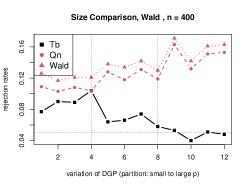
This section examines the finite sample properties of our bias corrected HLV-robust test $\mathcal{T}_{n}^{b}$ compared to the standard chi-square test $W_{n}$, which does not account for growing $p$, and the unscaled $\mathcal{Q}_{n}$ statistic with standard normal critical values, which does not account for $\mathcal{V}$, in terms of bias, size and power.

We will consider the examples below in our Monte Carlo experiments. In Appendix B we check our assumptions for these settings.

E1 (Multiple Regression of Growing Dimension).

Koenker (1988) found through his metastudy that it is common practice in econometrics to increase the number of regressors as the sample size $n$ grows, at a rate of roughly $O\left(n^{1/4}\right)$. In this case, the approximation error $r_{t}$ is not explicitly modeled and may be set as zero. Practitioners thus adopt a flexible approach to modelling, where the assumed model becomes richer with more covariates and with more lagged terms to account for the dynamic effect in the spirit of the distributed lag model, as illustrated in e.g. Stock and Watson (2015).

E2 (Infinite-Order Autoregression).

This model is one of the most fundamental models in time series analysis, see e.g. Brockwell et al. (1991) or Hamilton (2020). For the process to be stationary, the coefficients $\left\{b_{j}\right\}$ in the AR$\left(\infty\right)$ model $y_{t}=b_{0}+\sum_{j=1}^{\infty}b_{j}y_{t-j}+\varepsilon_{t}$ are assumed to obey a certain decay rate. Specifically, the tail sum of the coefficients satisfies Assumption 2 if $\sum_{j=p}^{\infty}\left|b_{j}\right|=o\left(n^{-1/2}\right)$. While we take $p$ as given in our analysis, for practical purposes various methods based on information criteria are available to choose the truncation lag $p$, see e.g. Shibata (1980) and references therein. Wang et al. (2007) propose a lasso-based autoregressive order selection rule while Lee et al. (2018) propose a lag selection rule in an infinite order panel autoregression. For expositional ease, we assume that the observations begin from $t=1-p$ and $x_{1}=(1,y_{0},...,y_{1-p})$.

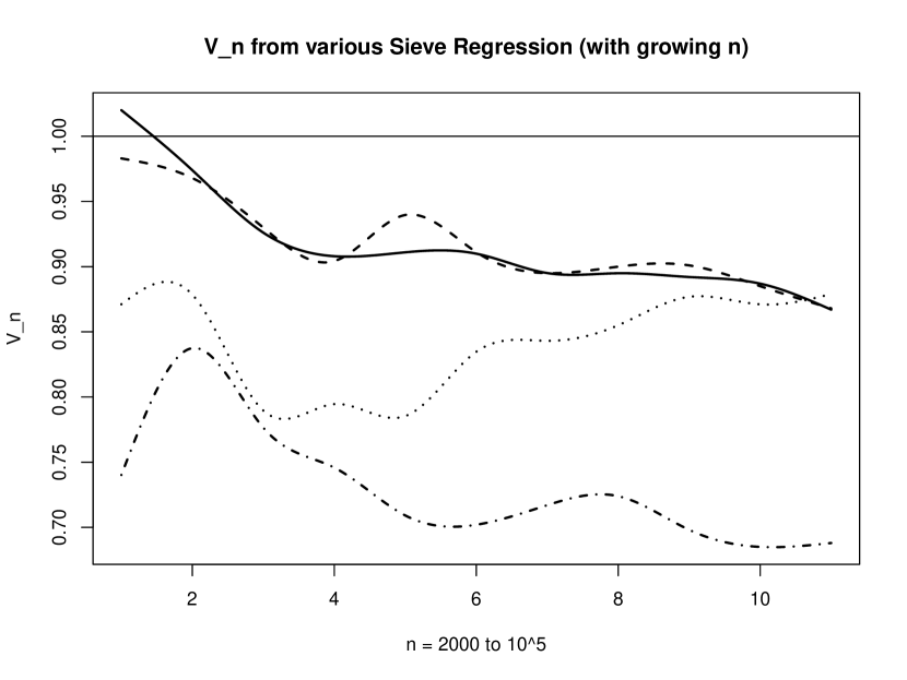
E3 (Nonparametric Series Regression).

In case of the nonparametric series least squares estimation of $E\left(y_{t}|z_{t}\right)$, there exists a sequence of transformations of the covariates $z_{t}$ given by $x_{nt}:=x_{n}\left(z_{t}\right):{\mathbb{R}}^{k}\mapsto{\mathbb{R}}^{p},$ and coefficients $\beta_{n}$ such that $E\left(y_{t}|\mathcal{F}_{t-1}\right)=f\left(z_{t}\right)=x_{nt}^{\prime}\beta_{n}+r_{n}\left(z_{t}\right),$ where $r_{nt}=r_{n}\left(z_{t}\right)$ meets Assumption 2 for a broad class of functions $f$, see e.g. Andrews (1991a), Newey (1997), Chen (2007) and Lee and Robinson (2016). By Lemma 1 of Lee and Robinson (2016), it is met if $|r_{t}|_{\infty}=O(p^{\alpha})$ for some $\alpha<0$ and $p^{2\alpha}\leq n^{-1}$. Depending on the smoothness of the nonparametric function $f(\cdot)$, the regressor support dimension $k$, and the type of basis functions used, different values of $\alpha$ may be implied, see e.g. Newey (1997), Chen (2007), p. 5573, for examples and further references. Often, the condition (2.2) holds under the so-called undersmoothing selection of $p$. Another closely related example is the partially linear regression model, e.g. Engle et al. (1986) and Robinson (1988). Again, while we do not consider data-dependent $p$, for practical purposes the literature proposes methods for the choice of $p$ using cross validation or information criteria, see e.g. p. 5623 of Chen (2007) for a list of references.

The tests are applied to the setting of the Chow test and testing general linear restrictions. We consider various sample sizes $n$ and dimensions $p$ from the three examples, E1-E3, with the error generated from a bounded ARCH process

(6.1) $$\varepsilon_{t}=\sigma_{t}\eta_{t},\;\;\;\;\;\;\;\;\;\;\;\;\;\sigma_{t}^{2}=\left(1-\alpha\right)+\alpha\phi(\varepsilon_{t-1}),$$

where $\phi(x)=x^{2}1\{|x|\leq c\}+c^{2}1\{|x|>c\}$, $\eta_{t}=\left(u_{t}-Eu_{t}\right)/\sqrt{var\left(u_{t}\right)}$, and $\left\{u_{t}\right\}$ is an iid sequence from the Marron and Wand (1992) normal mixture distributions of type 1-3, which we refer to as error 1, 2 and 3. Their error 1 is standard normal. For a standard normal vector $\left(Z_{1},...,Z_{k}\right)$ and multinomial vector $\left(d_{1},...,d_{k}\right)$ with probability $\left(1/5,1/5,3/5\right)$, error 2 skewed unimodal variate is $u_{t}=Z_{1}d_{1}+\left(2Z_{2}/3+1/2\right)d_{2}+d_{3}\left(5Z_{3}/9+13/12\right)$, while error 3 strongly skewed variate is $u_{t}=\sum_{l=0}^{7}d_{l+1}\left(Z_{l+1}\left(2/3\right)^{l}+3\left(\left(2/3\right)^{l}-1\right)\right)$ with equally likely $d_{i}$’s. We report results using (6.1) with $\alpha\in\left\{0.3,0.4,0.5,0.55,0.57\right\}$ and $c=2.5$. Results from $c=3$ and $\infty$ are similar and omitted.

More specifically, for multiple regression, E1, the regressors $x_{t}$ consist of independent AR(1) processes with coefficient $\alpha_{x}$ and ARCH innovation as in (6.1) and their lags of order up to 3. That is, we consider the distributed lag model with a growing number of variables. The first five elements of $\beta$ in (2.1) are set as $d_{0}\left(5^{-1/2},...,5^{-1/2}\right)p^{1/4}n^{-1/2}$ and the others as zeros. When there is a break, all the values become zero after the break so that the value $d_{0}$ controls the magnitude of the change. We vary $p\in\{5,9,13\}$ to examine the effect of the dimension on our tests.

For the infinite order AR regression, E2, we generate the sample from the MA(1) model $y_{t}=\varepsilon_{t}+\theta 1\left\{t\leq\mu\right\}\varepsilon_{t-1}$, with $\mu=n$ for the size experiment and $\mu=[n\gamma]$ for the power evaluation, and estimate the AR($p$) model with $p=9$ for $n=250$ and $p=13$ for $n=500$. For the sieve regression, E3, we consider two variables $\zeta_{1t}$ and $\zeta_{2t}$ and their lags $\zeta_{1,t-1}$ and $\zeta_{2,t-1}$ as regressors, denoted by $z_{1t},\cdots,z_{4t}$, after transforming them as $2\arctan\left(\zeta_{it}\right)/\pi$. Each $\zeta_{it}$ follows an AR(1) process with ARCH error. The regression function is set as $f\left(z_{1},\cdots,z_{4}\right)=d_{0}\left(1,z_{1},\cdots,z_{4},z_{1}^{2},...,z_{4}^{p_{1}}\right)\left(1^{-2},...,p_{2}^{-2}\right)^{\prime}+\sqrt{\left|z_{1}\right|/n}$ with $p_{1}=\left\lfloor n^{1/4}\right\rfloor$ and $p_{2}=1+4(p_{1}-1)$. To estimate the regression function, we construct $x_{t}$ from polynomial basis functions and its dimension $p=p_{2}$.

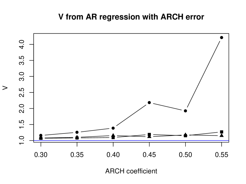
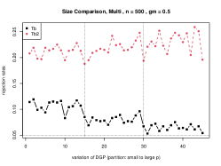
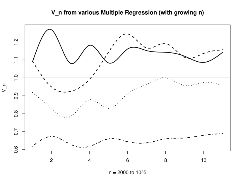
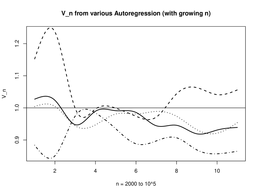
We first employ these DGPs to simulate pre-limit values of $\mathcal{V}$ in (3.2) with $n=m=500,l=0$ and $p$ as described above for each case, which are plotted in Figure 1, reporting averages from 10000 iterations. This serves as a useful illustration to observe visually that pre-limiting $\mathcal{V}$ deviates from unity for various specifications. A broad observation we make is that the deviation is bigger with larger ARCH coefficients and bigger autocorrelation in $x_{t}$, although this feature is not always monotone. To conclude, we observe that the nonlinear serial autocorrelation factor can induce serious distortion in inference without a suitable robustifying treatment, as we provide in section 4.2.

Also, Appendix B gives the verification of the high-level conditions in Assumptions 1-4 for these examples.

6.1. Chow Test

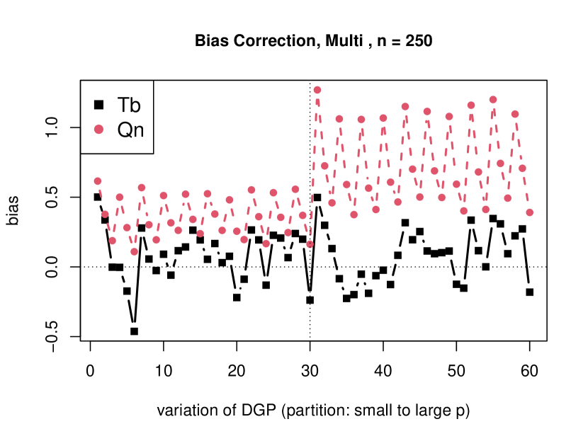
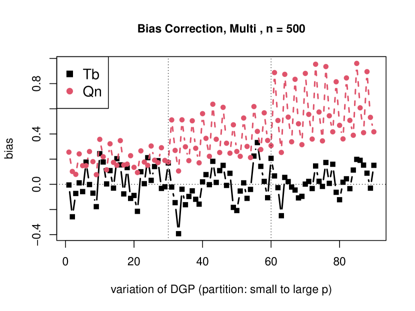
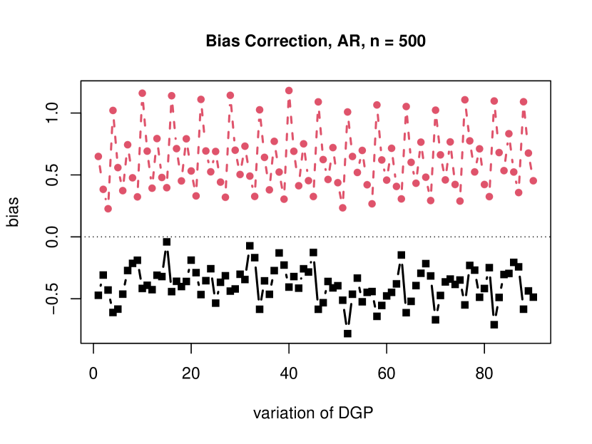
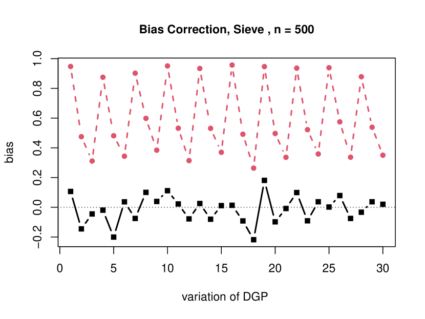
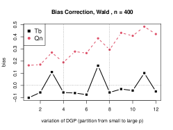
We consider three candidate break points as proportions of the sample sizes, $\gamma\in\{0.2,0.3,0.5\}$. We begin by examining the bias of $\mathcal{Q}_{n}(\gamma)$, conventionally centered by the degrees of freedom $p$, under the null hypothesis. Note that a severe bias in $\mathcal{Q}_{n}(\gamma)$ also implies that the size of the Wald test $W_{n}(\gamma)$ can be distorted severely. We report the results in Figure 2, in which the line with dot markers shows the bias in $\mathcal{Q}_{n}(\gamma)$ for $n=250$ and $n=500$. For E1, (Figures 2(a), 2(d)), each vertical partition (marked by a dotted vertical line) corresponds to a specific value of $p$. Within each vertical partition the DGP parameters change along the horizontal axes as $(\text{error type},\alpha)$, in lexicographic order. As $p$ grows, we observe that the $\mathcal{Q}_{n}\left(\gamma\right)$ statistic exhibits severe finite sample bias for all values of the DGP parameters.

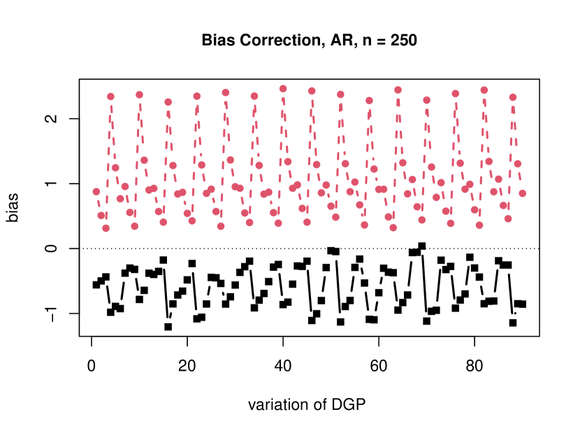
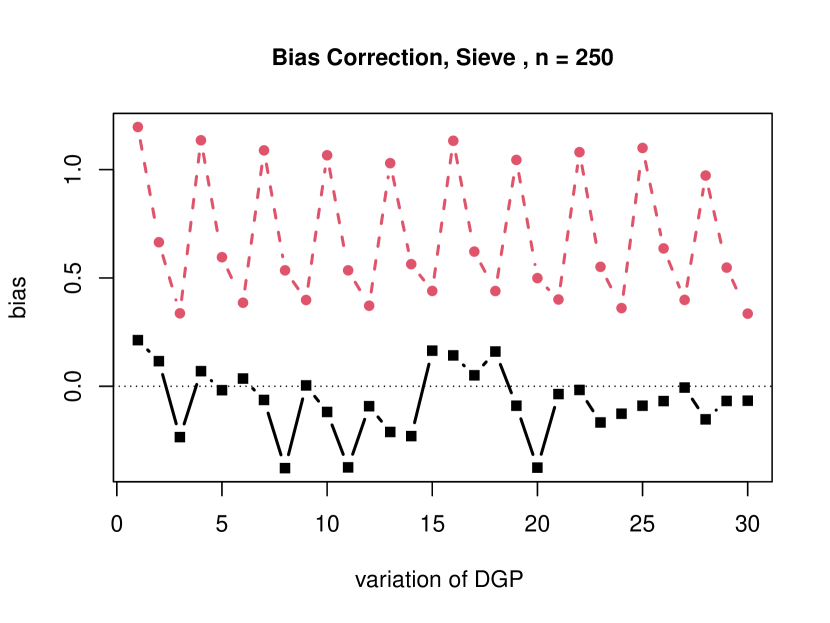
A similar visualization of bias in $\mathcal{Q}_{n}(\gamma)$ for E2 is presented in Figures 2(b), 2(e). Rather than report values for different $p$, here we focus on the case $p=9$ for $n=250$ and $p=13$ for $n=500$ and allow the values of $\alpha$ and $\theta$ to vary along the horizontal axis lexicographically as $(\text{error type},\alpha\text{ or }\theta)$, as detailed in the caption. A substantial bias in $\mathcal{Q}_{n}(\gamma)$ is observed for all cases, regardless of $n=250$ or $n=500$, albeit the biases are generally smaller in the latter case. Finally, Figures 2(c), 2(f) show the bias in $\mathcal{Q}_{n}(\gamma)$ for E3, with the same $p$ as for E2, to mimic the asymptotic regime of a sieve regression, and parameters as in E2. We observe a similar pattern of substantial bias for both sample sizes.

As discussed above, Figures 2(a)-2(f) clearly show that the biases present in $\mathcal{Q}_{n}\left(\gamma\right)$ are severe. In these figures we also plot the bias of the bias-corrected HLV-robust statistic $\mathcal{T}^{b}_{n}(\gamma)$, shown in black with square markers. The bootstrap bias correction seems to work well for all the cases, substantially alleviating bias. In Figure 2, we observe that $\mathcal{T}^{b}_{n}(\gamma)$ can still exhibit some bias for specific cases but for E1 and E3, unlike the bias of $\mathcal{Q}_{n}(\gamma)$, this is centered around zero, while for E2 it is generally smaller in absolute value. Thus we recommend the use of the bootstrap bias correction in practice especially when faced with large values of $p$.

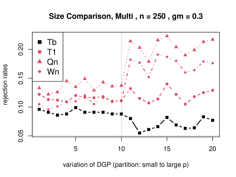
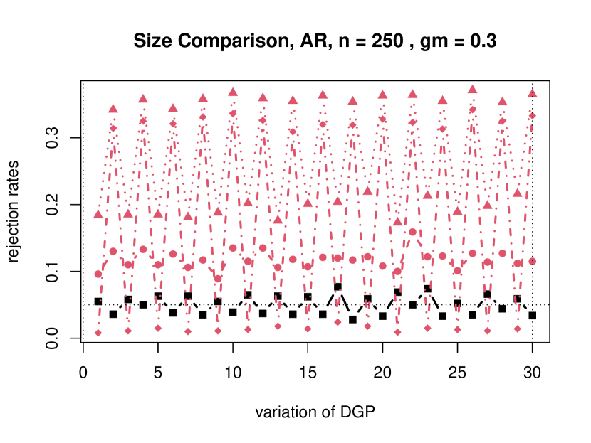
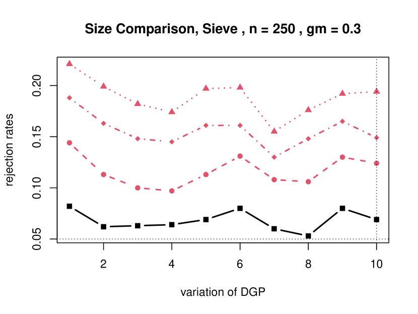
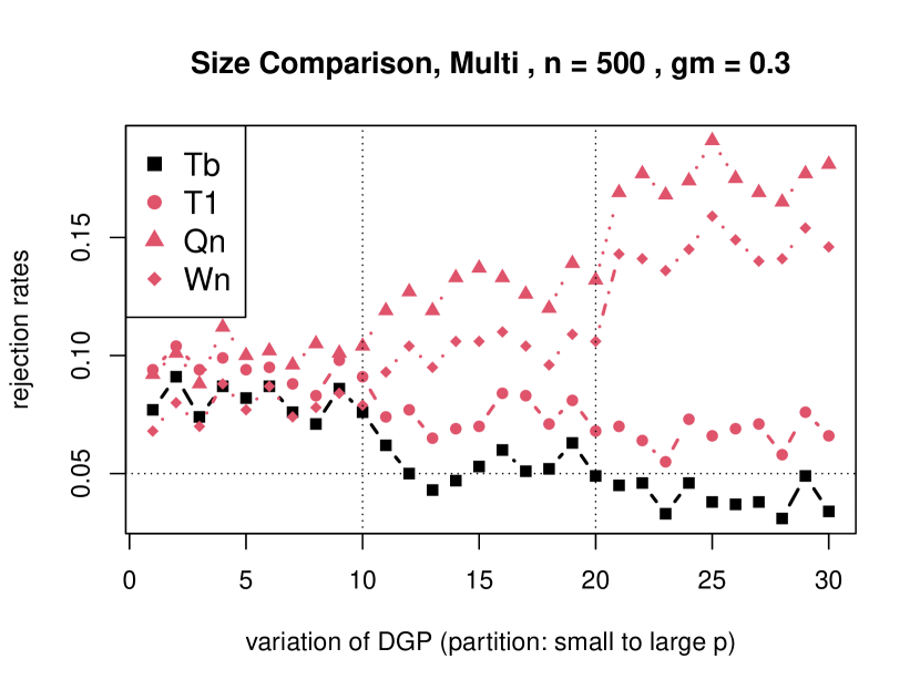
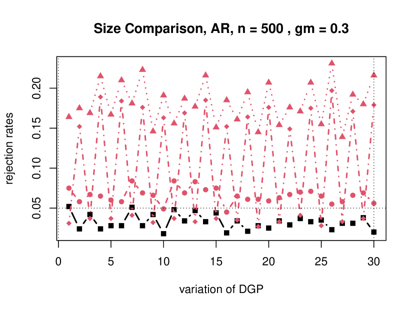
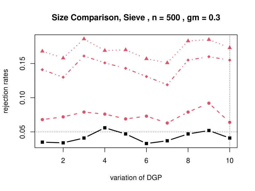
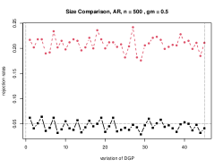
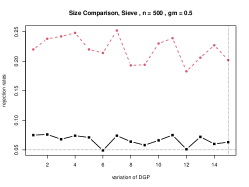
We now study the finite sample rejection frequencies of four competing tests: $\mathcal{T}_{n}^{b}(\gamma),\mathcal{T}_{n}(\gamma),\mathcal{Q}_{n}(\gamma),$ and $W_{n}(\gamma)$, with specific parameter values as given in the respective figure captions. As shown earlier, the unknown HLV scaling factor $\mathcal{V}$ varies along different ARCH parameters. This motivates our approach of experimenting with different $\alpha$ values and innovations. The Monte Carlo sizes resulting from the experiment are plotted in Figure 3, wherein we place a horizontal dotted line to mark the nominal size of 5%. We report results for $\gamma=0.3$. The vertical partitions in each panel of Figure 3 correspond, as discussed earlier, to increasing values of $p$ from left to right in E1. We cover multiple regression (Figures 3(a), 3(d)), AR fits (Figures 3(b), 3(e)) and sieve regression (Figures 3(c), 3(f)) for $n=250,500$.

For all DGPs, the usual Wald statistic $W_{n}(\gamma)$ (diamond markers) over-rejects. Simply standardizing the test statistic $W_{n}(\gamma)$ to $\mathcal{Q}_{n}(\gamma)$, hence ignoring the HLV $\mathcal{V}$, does not improve matters. In fact, it usually worsens the problem of over-rejection. This can be seen in the lines with triangle markers. Our HLV-robust statistic $\mathcal{T}_{n}(\gamma)$ does much better, as the lines with dot markers indicate. While this shows the importance of the correction for $\mathcal{V}$ that we stress in the paper, there is still a tendency to over-reject. On the other hand, applying the bootstrap bias correction and using the bias corrected HLV-robust statistic $\mathcal{T}_{n}^{b}(\gamma)$ achieves excellent size control, as can be seen in the line with square markers. The discussion holds regardless of whether $n=250$ or $n=500$. Thus the importance of our proposed testing procedure is clearly visible.

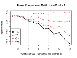
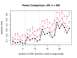
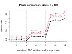
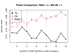
We now analyze the power features of the competing test statistics for the proposed DGPs, allowing for breaks of different magnitudes and setting $\gamma=0.5$. After the break all the coefficients become zero so that the values of $d_{0}$ govern the size of the breaks in E1 and E3, while the values of $\theta$ do so for E2. The power performance is plotted in Figure 4, where to conserve space we report results only for $n=400$. Again, we use $p=9$ for E2 and E3, while a range of $p$ is employed for E1. The line marker schemes for each of the competing tests are as described earlier. Examining the figure, the power of our HLV-robust statistics $\mathcal{T}_{n}(\gamma)$ (dots) and $\mathcal{T}_{n}^{b}(\gamma)$ (squares) tracks that of the uncorrected ones as the break size increases for both E2 (center panel) and E3 (right panel). For E1 (left panel), we only report results for $d_{0}=2$ for clarity. We observe that $W_{n}(\gamma)$ tends to have the highest power but our statistics still perform reasonably well with power in excess of 80% even for large $p$. Recall that our size experiments earlier indicate that $W_{n}(\gamma)$ over-rejects, a phenomenon of which high power is likely an artefact. Thus we conclude that our test is able to control size without sacrificing power to an undue extent.

Finally, Figure 5 reports the size distortions when the sample variance of $q_{t}$ multiplied by 2 is employed instead of $\hat{\mathcal{V}}$, noting that $q_{t}$ is a martingale difference array. While we discussed the potential reasons for this severe size distortion in Section 4.2, the investigation on a more precise approximation to the finite sample distribution of this statistic is an interesting issue but out of the scope of this paper due to the complex nature of the statistic. Nevertheless, Figure 5 provides numerical evidence that the typical scaling by variance is not sufficient to control size. Specifically, define the test statistic $\mathcal{T}_{n}^{b,2}(\gamma)$ exactly like $\mathcal{T}_{n}^{b}(\gamma)$ but with random scaling replaced by twice the variance of $q_{t}$ and the standard normal approximation. It is clear that the test (triangle markers) is oversized relative to our recommended test $\mathcal{T}_{n}^{b}(\gamma)$.

6.2. Testing Linear Restrictions

This section presents the outcomes of bias, size and power experiments for testing general linear restrictions, analogous to those for the Chow test in the preceding discussion. We use the reparameterization of the linear restrictions to the exclusion restrictions ${\delta}_{2}=0$, as discussed in Section 5. We focus on E1 with $n=400$, $p=8,12,16$, $d_{0}=1$, error 1 and 2 disturbances and $\alpha=0.4,0.55$. The results are displayed in Figure 6, with the same marking scheme as before and three test statistics employed: $W_{n}^{e}$, $\mathcal{Q}_{n}^{e}$ and $\mathcal{T}_{n}^{e,b}$. In all three figures, each vertical partition marks a different value of $p$, increasing from left to right.

The left panel of Figure 6 shows that the bootstrap bias correction indeed improves matters, as was the case for the Chow test. The center panel again demonstrates the importance of our proposed corrections for size control. $W_{n}^{e}$ and $\mathcal{Q}_{n}^{e}$ tend to over-reject, becoming worse as $p$ increases. $\mathcal{T}_{n}^{e,b}$ controls size very well for medium to large $p$, while still outperforming $W_{n}^{e}$ and $\mathcal{Q}_{n}^{e}$ for smaller $p$. The right panel shows that $\mathcal{T}_{n}^{e,b}$ sacrifices some power relative to $W_{n}^{e}$ and $\mathcal{Q}_{n}^{e}$, but not unduly so.

7. Empirical example

We revisit structural stability in the Hamilton (2003) study of the effect of oil shocks on economic activities. The autoregressive distributed lag model, ADL$(p,p)$, with quarterly time series of outputs and several oil price measures is employed. For real output, the quarterly growth rate of chain-weighted real GDP is used, while the oil price is the nominal crude oil producer price index, seasonally unadjusted. As in Hamilton, three oil price measures were considered: the growth rate $o_{t}$ from the previous quarter, the rectified linear unit, $o_{t}^{+}=o_{t}1\left\{o_{t}>0\right\}$, and the net oil price increase, $o_{t}^{n}$, defined as the amount by which log oil prices in quarter $t$ exceed their peak value over the previous 12 months. If it does not exceed the previous peak, then $o_{t}^{n}$ is taken to be zero. We extend the original sample using the FRED database at the St. Louis Fed to obtain a sample from January 1949 to October 2019.

First, we re-evaluate structural stability of the GDP dynamics using AR$(p)$ fits, and that of the regression function of GDP growth on oil price change using an ADL$(p,p)$ model with the three alternative measures of oil price change. Following Table 4 in Hamilton (2003), we investigate four exogenous disruptions in world petroleum supply. These are: the Arab–Israel War (November 1973), the Iranian Revolution (November 1978), the Iran–Iraq War (October 1980) and the Persian Gulf War (August 1990).

The p-values of the tests are reported in sub-tables (a) and (b) in Table 1, where for $W(\gamma)$ these are computed using the ordinary Chow test. We observe that in many cases the usual Chow test supports a structural break in both regressions more strongly than our recommended $\mathcal{T}^{b}_{n}(\gamma)$ test. Thus, the evidence for structural instability is often no longer as strong. In fact, the p-values that we calculate using our test exceed those of the standard Chow test in 22 out of 32 cases.

	Stability test								Exclusion test
	(a) AR($p$)		(b) ADL($p,p$)						(c) ADL($p,p$)
GDP			$o_{t}$		$o_{t}^{+}$		$o_{t}^{n}$		all oil			NL
lags $p$	4	6	4	6	4	6	4	6		4	6	4	6
	Arab-Israel War, November 1973
$\mathcal{T}_{n}^{b}(\gamma)$	51.3	43.9	3.5	0.52	1.64	1.33	1.58	0	$\mathcal{T}_{n}^{e,b}$	8.7	26.9	7.6	19
${W}_{n}(\gamma)$	52.9	38	0.5	0	0.58	0	0.7	0	$W_{n}^{e}$	9	4.4	2.8	4.4
	Iranian Revolution, November 1978
$\mathcal{T}_{n}^{b}(\gamma)$	41.8	52.8	1.04	0.03	7	0.1	0	0
${W}_{n}(\gamma)$	48.5	53.2	0.6	0	7.57	0	0.1	0
	Iran-Iraq War, October 1980
$\mathcal{T}_{n}^{b}(\gamma)$	13.1	28.2	0.3	0.4	0.33	0.64	0.33	0
${W}_{n}(\gamma)$	10.6	19.7	0	0	0.1	0	0	0
	Persian Gulf War, August 1990
$\mathcal{T}_{n}^{b}(\gamma)$	54.6	53.6	73.3	43.7	17.8	31.2	4.53	4.85
${W}_{n}(\gamma)$	56.2	65	39.5	16	17.1	14.4	1.9	1.17

Table 1. $100\times$p-values of Chow tests and exclusion restriction tests for full sample. (a) Tests for stability of GDP dynamics via AR$(p)$ fits. (b) Tests for stability of ADL$(p,p)$ regressions of GDP on $o_{t}$, $o_{t}^{+}$ or $o_{t}^{n}$. (c) Tests for exclusion restrictions on all oil price measures ($o_{t}$, $o_{t}^{+}$, $o_{t}^{n}$) or nonlinear oil price measures ($o_{t}^{+}$, $o_{t}^{n}$.) in ADL$(p,p)$ regressions of GDP on oil prices.

	Stability test								Exclusion test
	(a) AR($p$)		(b) ADL($p,p$)						(c) ADL($p,p$)
IP			$o_{t}$		$o_{t}^{+}$		$o_{t}^{n}$		all oil			NL
lags $p$	12	18	12	18	12	18	12	18		12	18	12	18
	Arab-Israel War, November 1973
$\mathcal{T}_{n}^{b}(\gamma)$	20.9	32.9	33.9	28.4	24.9	18.9	10.6	17.8	$\mathcal{T}_{n}^{e,b}$	27	30.9	11.9	18.5
${W}_{n}(\gamma)$	8.46	26.4	5.18	1.71	3.93	0.78	1.23	1.65	$W_{n}^{e}$	1.7	0.8	0.5	0.5
	Iranian Revolution, November 1978
$\mathcal{T}_{n}^{b}(\gamma)$	11	21.5	1.39	0.74	0.7	0.26	0.15	0.04
${W}_{n}(\gamma)$	0.96	4.3	0	0	0	0	0	0
	Iran-Iraq War, October 1980
$\mathcal{T}_{n}^{b}(\gamma)$	3.31	9.34	1.96	1.87	1.15	1.68	0.08	0.46
${W}_{n}(\gamma)$	0	0.04	0	0	0	0	0	0
	Persian Gulf War, August 1990
$\mathcal{T}_{n}^{b}(\gamma)$	5.82	14.6	3.95	19.4	2.03	12.8	0.94	8.04
${W}_{n}(\gamma)$	0.08	1.13	0.21	2.98	0.23	2.43	0.02	0.22

Table 2. $100\times$p-values of Chow tests and exclusion restriction tests for full sample. (a) Tests for stability of IP dynamics via AR$(p)$ fits. (b) Tests for stability of ADL$(p,p)$ regressions of IP on $o_{t}$, $o_{t}^{+}$ or $o_{t}^{n}$. (c) Tests for exclusion restrictions on all oil price measures ($o_{t}$, $o_{t}^{+}$, $o_{t}^{n}$) or nonlinear oil price measures ($o_{t}^{+}$, $o_{t}^{n}$.) in ADL$(p,p)$ regressions of IP on oil prices.

Second, we explore the relevance of the oil price measures and of the nonlinear transformations ($o_{t}^{+}$, $o_{t}^{n}$) by testing two exclusion restrictions in the ADL$(p,p)$ regression that include all the three oil price measures as covariates. The first exclusion restriction is to set the coefficients of all the measures as zero and the second is to set those of the nonlinear transformations ($o_{t}^{+}$, $o_{t}^{n}$) to zero. This yields 12 and 8 df, respectively, when $p=4$ and 18 and 12 df, respectively, when $p=6$. As shown in sub-table (c) of Table 1, our recommended test $T^{e,b}_{n}$ produces p-values bigger than 5% for all cases, suggesting the effect of oil price as measured by these transformations is not statistically significant, nor are the nonlinear transformations. The standard Wald test for the exclusion restrictions is more supportive of their inclusion but may lack robustness with large df. Overall, our tests produce larger p-values than the standard Chow or Wald tests in 72% of cases (26 out of 36) cases in Table 1.

As another measure of economic activity we now consider the industrial production (IP) index. This is available at monthly frequency and thus we consider ADL(12,12) and ADL(18,18) to include lags of one year and one and a half years, respectively. With monthly data, the dimensionality becomes more important: the number of restrictions we test varies from 13 and 25 in the structural break test for the AR(12) and ADL(12,12) regressions to 36 and 48 for the exclusion tests in the ADL(18,18) regression.

The results in Table 2 illustrate much stronger differences in the conclusions of our test versus the standard Chow test, compared to the GDP study in Table 1. The rejection of the null of no structural break is now often overturned at reasonable significance levels. For example, for the Arab-Israel War, the ADL$(p,p)$ model fails to reject the null of no structural break for any significance level below 10.6% when using our test $\mathcal{T}^{b}_{n}(\gamma)$, in contrast to the standard Chow test ${W}_{n}(\gamma)$. Conclusions are likewise overturned for the AR$(p)$ model and the Iranian Revolution and Iran-Iraq War, and indeed for both the ADL$(p,p)$ and AR$(p)$ in several cases for the Persian Gulf War.

The results in Tables 1 and 2 are not surprising given our simulation evidence. Indeed, our Monte Carlo simulation illustrates the effect of the degrees of freedom (df) on finite sample properties of the two tests, $W_{n}(\gamma)$ tends to have larger p values in the AR case ($p+1$ df) than in the ADL case ($2p+1$ df), while $\mathcal{T}^{b}_{n}(\gamma)$ would be the opposite. These are exactly the patterns that we also observe. Finally, sub-table (c) of Table 2 shows even stronger differences than Table 1(c), with all conclusions on the exclusion restrictions overturned at significance levels below 11.6%. Overall, our tests produce larger p-values in every single case considered in Table 2 when compared to the standard Chow or Wald tests.

(a) E1 with $p=12,\alpha_{x}=0.7$

(b) E2 with $p=12,\theta=-0.5$.

(c) E3 with $p=13,\alpha_{x}=0.7$

Figure 1. Simulated pre-limit of $\mathcal{V}$ for $n=m=500$ and $l=0$. Error 1: square; Error 2: dot; Error 3: triangle.

(a) Chow test bias, E1: $n=250$.

(b) Chow test bias, E2: $n=250$.

(c) Chow test bias, E3: $n=250$.

(d) Chow test bias, E1: $n=500$.

(e) Chow test bias, E2: $n=500$.

(f) Chow test bias, E3: $n=500$.

Figure 2. Bias in $\mathcal{Q}_{n}(\gamma)$ (dot) and $\mathcal{T}_{n}^{b}(\gamma)$ (square, black). For E1, the vertical partitions in (a) and (d) correspond to $p=5,9$ and $p=5,9,13$, respectively. Within each vertical partition results are ordered lexicographically as $(\gamma\in\{0.2,0.3,0.5\},\text{error }\in\{1,2\},\alpha\in\{0.3,0.57\})$. E2 and E3: $p=9$ for $n=250$ and $p=13$ for $n=500$. Results horizontally ordered lexicographically as $(\gamma,\text{error },\alpha\text{ or }\theta)$.

(a) Chow test size, E1: $n=250$, $\gamma=0.3$.

(b) Chow test size, E2: $n=250$, $\gamma=0.3$.

(c) Chow test size, E3: $n=250$, $\gamma=0.3$.

(d) Chow test size, E1: $n=500$, $\gamma=0.3$.

(e) Chow test size, E2: $n=500$, $\gamma=0.3$.

(f) Chow test size, E3: $n=500$, $\gamma=0.3$.

Figure 3. Size of Chow tests with $\gamma=0.3$ : ${W}_{n}(\gamma)$ (diamond), $\mathcal{Q}_{n}(\gamma)$ (triangle), $\mathcal{T}_{n}(\gamma)$ (dot) and $\mathcal{T}_{n}^{b}(\gamma)$ (square, black). Nominal size is 5%. For E1, vertical partitions in (a) correspond to $n=250$ and $p=5,9$ and those in (d) correspond to $n=500$ and $p=5,9,13$. Within each vertical partition results are ordered lexicographically as $(\text{error }\in\{1,2\},\alpha\in\{0.3,0.57\})$. For E2, $p=9$ for $n=250$ and $p=13$ for $n=500$. Results horizontally ordered lexicographically as $(\text{error }\in\{1,2\},\alpha\in\{0.3,0.57\}\text{ or }\theta\in\{-0.5,-0.1,0.5\})$. For E3, $p=9$ for $n=250$ and $p=13$ for $n=500$. Results horizontally ordered lexicographically as $(\text{error }\in\{1,2\},\alpha\in\{0.3,...,0.57\})$.

Figure 4. Power of Chow tests, ${W}_{n}(\gamma)$ (diamond), $\mathcal{Q}_{n}(\gamma)$ (triangle), $\mathcal{T}_{n}(\gamma)$ (dot) and $\mathcal{T}_{n}^{b}(\gamma)$ (square, black): E1 (left), E2 (center) and E3 (right), $n=400$, $\gamma=0.5$. Vertical partitions correspond to $p=5,9,13$ (left), $\theta=0.2,0.4,0.6,0.8$ (center) and $\delta=0.5p^{1/4}/n^{1/2}(1,5,10)$ (right). Within each vertical partition results are ordered lexicographically as $(\text{error }\in\{1,2,3\},\alpha\in\{0.3,0.5\})$ for E1 and $(\text{error }\in\{1,2,3\},\alpha\in\{0.3,0.5\}\text{ or }\theta)$ for E2 and E3.

Figure 5. Size distortions in the test based on $\mathcal{T}_{n}^{b,2}(\gamma)$, which is computed exactly like $\mathcal{T}_{n}^{b}(\gamma)$ except that the scaling is done by the sample variance of $q_{t}$ along with the standard normal approximation.

Figure 6. Bias, Size, and Power of Exclusion Tests in E1: $\mathcal{Q}_{n}^{e}$ (dot) and $\mathcal{T}_{n}^{e,b}$ (square, black). Left to right: vertical partitions correspond to $p=8,12,16$. Within each vertical partition results are ordered lexicographically as $(\text{error }\in\{1,2\},\alpha\in\{0.4,0.55\})$.

Appendix A Proofs of theorems

We begin with some notation. Let

$$A(\gamma)=\left(X^{\ast}(\gamma)^{\prime}M_{X}X^{\ast}(\gamma)\right)^{-1}X^{\ast}(\gamma)^{\prime}M_{X}$$

with $X^{\ast}(\gamma)$ having $t$-th row $x_{t}^{\ast}(\gamma)^{\prime}=x_{t}^{\prime}1\left\{t/n>\gamma\right\}$, $M_{X}$ the residual maker for the matrix $X$ with $t$-th row $x_{t}^{\prime}$, and

$$B(\gamma)=RM(\gamma)^{-1}\Omega(\gamma)M(\gamma)^{-1}R^{\prime}.$$

Also, let $\bar{\Omega}(\gamma)=n^{-1}\sum_{t=1}^{n}x_{t}(\gamma)x_{t}^{\prime}(\gamma)\sigma_{t}^{2}$ and $x_{t}(\gamma)=\left(x_{t}^{\prime},x_{t}^{\prime\ast}(\gamma)\right)^{\prime}$. It is also convenient to recall that $\hat{M}=n^{-1}X^{\prime}X$ and define $\hat{S}(\gamma)=n^{-1}X^{\prime\ast}(\gamma)X(\gamma)$. Recall that cross-referenced items prefixed with ‘S’ can be found in the online supplementary appendix.

A.1. Proofs for Section 3

Proof of Theorem 3.1 and 3.2.

For the convenience of exposition, these are combined with the proof of Theorem 4.1 in the next section.    

A.2. Proof of Theorem 4.1:

For the result under the null, Section A.2.1 first establishes the asymptotic normality for ${\mathcal{Q}}_{n}(\gamma),$ and then Section A.2.2 proves $\hat{\mathcal{V}}\overset{d}{\to}\int_{0}^{1}\int_{0}^{1}K_{h}^{*}\left(r,s\right)dW\left(r\right)dW\left(s\right)$, where $W(r)$ denotes the same limit Gaussian process as in Theorem ST.B.2. Then, the claim follows by Theorem ST.B.2 and the continuous mapping theorem. After completing the proof under the null, we prove convergence under the local alternative in Section A.2.4.

A.2.1. Asymptotic normality of ${\mathcal{Q}}_{n}(\gamma)$ under $\mathcal{H}_{0}$.

Proof.

This step is quite involved and we delegate proofs of many intermediate steps to Section S.B. Summarizing these steps, Theorem ST.B.1 therein develops the initial approximation ${\mathcal{Q}}_{n}(\gamma)=\left({{\mathcal{R}}_{n}(\gamma)-p}\right)/{\sqrt{2p}}+o_{p}(1)$, where $\mathcal{R}_{n}(\gamma)$ is defined in (3.4). Then, (SB.45) and Lemma SL.B.8 yield the second approximation

$$\frac{{\mathcal{R}}_{n}(\gamma)-p}{\sqrt{2p}}={{\mathcal{S}}_{n}(\gamma)}+o_{p}(1),$$

where

(A.1) $${\mathcal{S}}_{n}(\gamma)=\frac{n^{-1}\sum_{s\neq t}g_{t}(\gamma)^{\prime}\Omega^{-1}g_{s}(\gamma)\varepsilon_{t}\varepsilon_{s}}{\gamma\left(1-\gamma\right)\sqrt{2p}},$$

and $g_{t}(\gamma)=x_{t}1\left\{t/n\leq\gamma\right\}-\gamma x_{t}$. The claim now follows by a CLT for $\mathcal{S}_{n}(\gamma)$ established in Theorem ST.B.2.    

A.2.2. Weak convergence of $\hat{\mathcal{V}}$

Proof.

First, we establish tightness of the stochastic process

$$\mathcal{A}_{n}(\gamma)=\frac{1}{n\sqrt{p}}{\sum_{s=2}^{[n\gamma]}}{\sum_{t=1}^{s-1}}\xi_{t}^{\prime}\xi_{s},$$

with $\xi_{t}=\left\{\xi_{ti}\right\}_{i=1}^{p}=\Omega^{-1/2}x_{t}\varepsilon_{t}$ being an mds.

Note that $\mathcal{A}_{n}\left(\gamma\right)$ is a partial sum process of a heterogeneous martingale difference array $w_{ns}=\xi_{s}^{\prime}{\sum_{t=1}^{s-1}}\xi_{t}/\sqrt{np}$, and thus it is sufficient to show

$$E\left|\mathcal{A}_{n}\left(\gamma_{1}\right)-\mathcal{A}_{n}\left(\gamma_{2}\right)\right|^{4} = E\left|\frac{1}{\sqrt{n}}{\sum_{s=\left[n\gamma_{1}\right]+1}^{[n\gamma_{2}]}}w_{ns}\right|^{4}$$

$$\leq E\left(\sum_{s}\mathrm{E}\left(w_{ns}^{2}|\mathcal{G}_{s-1}\right)/n\right)^{2}+n^{-1}\max_{s}E\left|w_{ns}\right|^{4}O\left(\left|\gamma_{2}-\gamma_{1}\right|\right)$$

$$= O\left(\left|\gamma_{2}-\gamma_{1}\right|\right),$$

where we apply the Rosenthal inequality, e.g. Hall and Heyde (1980), for the inequality and a calculation similar to (SB.11) and (SB.14) for the last equality. Specifically,

(A.3) $$n^{-1}\max_{s}E\left|w_{ns}\right|^{4}\leq\max_{s}E\left(E((\xi_{s}^{\prime}\xi_{s})^{2}|\mathcal{G}_{s-1})\left(\sum_{t_{1},t_{2}<s}\xi_{t_{1}}^{\prime}\xi_{t_{2}}\right)^{2}\right)n^{-3}p^{-2}=o(1),$$

by Assumption 4 and the same reasoning as for (SB.12) and (SB.14).

Having established tightness, by Lemma 1 (c) of Sun (2014) weak convergence follows if

(A.4) $$\hat{\mathcal{V}}-\tilde{\mathcal{V}}=o_{p}(1),$$

where $\tilde{\mathcal{V}}=\frac{2}{n}\text{$\sum_{t=2}^{n}\text{$\sum_{s=2}^{n}k\left(\frac{t-s}{n/h}\right)\bar{q}^{\star}_{s}$}\bar{q}^{\star}_{t}$},$ $q^{\star}_{t}=\left(np\right)^{-1/2}x_{t}^{\prime}{\Omega}^{-1}{\varepsilon}_{t}\text{$\sum_{s=1}^{t-1}x_{s}{\varepsilon}_{s}$}$, $\bar{q}^{\star}_{t}=q^{\star}_{t}-n^{-1}\sum_{t=2}^{n}q^{\star}_{t}$. Strictly speaking, Sun’s Lemma 1 (c) is stated for the case where the partial sums of $q_{t}$ are approximated by the partial sums of $e_{t}$, which is iid normal, but it also holds when it is approximated by the partial sums of $a_{nt}e_{t}$ for any real bounded array $a_{nt}$ by repeating the same argument in the proof. In our case, $a_{nt}=\sqrt{t/n}$.

Let $\varsigma=n/h$, $\hat{\zeta}_{t}=\hat{h}_{t}^{\prime}\sum_{s<t}\hat{h}_{s}/\sqrt{p}=\sqrt{n}q_{t}$, $\hat{h}_{t}=\hat{\Omega}^{-1/2}x_{t}\hat{e}_{t}$, $\bar{\hat{\zeta}}/\sqrt{n}=n^{-1}\sum_{t=2}^{n}q_{t}=n^{-1}\sum_{t=2}^{n}\hat{\zeta}_{t}/\sqrt{n}$, with analogous definitions using $\Omega$ and $\varepsilon_{t}$ for $\zeta_{t}$, $h_{t}$ and $\bar{\zeta}$. Then

(A.5) $$\hat{{\mathcal{V}}}-\tilde{{\mathcal{V}}} = n^{-2}\sum_{j=-(n-1)}^{n-1}k\left(j/\varsigma\right)n^{-1}\sum_{t=1+\left(j\vee 0\right)}^{n-\left|j\wedge 0\right|}\left\{\left(\hat{\zeta}_{t}\hat{\zeta}_{t+|j|}-\zeta_{t}\zeta_{t+|j|}\right)+2\bar{\hat{\zeta}}\left(\hat{\zeta}_{t}-\zeta_{t}\right)\right.$$

$$+ \left.\left(\bar{\hat{\zeta}}-\bar{\zeta}\right)\hat{\zeta}_{t}+\left(\bar{\hat{\zeta}}^{2}-\bar{\zeta}^{2}\right)\right\}.$$

We obtain a bound for

(A.6) $$\hat{\zeta}_{t}\hat{\zeta}_{t+|j|}-\zeta_{t}\zeta_{t+|j|}=\left(\hat{\zeta}_{t}-\zeta_{t}\right)\hat{\zeta}_{t+|j|}+\left(\hat{\zeta}_{t+|j|}-\zeta_{t+|j|}\right)\hat{\zeta}_{t},$$

while omitting similar details for the other three terms. To find a bound for (A.6), first note that $\left\|\hat{h}_{t}\right\|=O_{p}\left(\left\|x_{t}\right\|\right)=O_{p}\left(\sqrt{p}\right)$, by Assumption 3$(ii)$ and finite fourth moments of $x_{t}$ components (Assumption 3$(i)$), and because

(A.7) $$\hat{e}_{t}=y_{t}-x_{t}^{\prime}\hat{\delta_{1}}(\gamma)=x_{t}^{\prime}\left(\hat{\delta}_{1}(\gamma)-\delta_{1}\right)+x_{t}^{\prime}1\left(t/n>\gamma\right)\delta_{2\ell}+r_{t}+\varepsilon_{t}=O_{p}(1).$$

Hence

(A.8) $$\hat{\zeta}_{t}=\hat{h}_{t}^{\prime}\sum_{s<t}\hat{h}_{s}/\sqrt{p}=O_{p}\left(n\sqrt{p}\right).$$

By the same argument, $\left\|h_{t}\right\|=O_{p}(\sqrt{p})$ and $\zeta_{t}=O_{p}\left(n\sqrt{p}\right)$ as well.

Now recall that $\hat{e}_{t}-\varepsilon_{t}=x_{t}^{\prime}\left(\hat{\delta}_{1}(\gamma)-\delta_{1}\right)+x_{t}^{\prime}1\left(t/n>\gamma\right)\delta_{2\ell}+r_{t}$ and $\left\|\hat{\delta}_{1}(\gamma)-\delta_{1}\right\|=O_{p}\left(\left\|\hat{\delta}(\gamma)-\delta\right\|\right)=O_{p}\left(\lambda_{n}^{-1}\sqrt{p}/\sqrt{n}\right)$ implying that

(A.9) $$\hat{e}_{t}-\varepsilon_{t}=O_{p}\left(\max\left\{\lambda_{n}^{-1}p/\sqrt{n},p^{3/4}/\sqrt{n}\right\}\right).$$

Thus we obtain

(A.10) $$\left\|\hat{h}_{t}-h_{t}\right\|=\left\|\Omega^{-1}\left(\Omega-\hat{\Omega}\right)\hat{\Omega}^{-1}x_{t}\hat{e}_{t}+\Omega^{-1}x_{t}\left(\hat{e}_{t}-\varepsilon_{t}\right)\right\|=O_{p}\left(\lambda_{n}^{-2}\sqrt{p}\max\left\{v_{p},p/\sqrt{n}\right\}\right),$$

using Assumption 3$(iii)$. Using (A.10), we get

(A.11) $$\hat{\zeta}_{t}-\zeta_{t}=\left(\hat{h}_{t}-h_{t}\right)^{\prime}\sum_{s<t}\hat{h}_{s}/\sqrt{p}+\hat{h}_{t}^{\prime}\sum_{s<t}\left(\hat{h}_{s}-h_{s}\right)/\sqrt{p}=O_{p}\left(\lambda_{n}^{-2}n\sqrt{p}\max\left\{v_{p},p/\sqrt{n}\right\}\right).$$

Using (A.8) and (A.11) in (A.6), we obtain $\hat{\zeta}_{t}\hat{\zeta}_{t+|j|}-\zeta_{t}\zeta_{t+|j|}=O_{p}\left(\lambda_{n}^{-2}n^{2}p\max\left\{v_{p},p/\sqrt{n}\right\}\right)$. This, along with similarly obtained bounds for the remaining terms in (A.5) and Lemma 1 of Jansson (2002), yield

$$\hat{{\mathcal{V}}}-\tilde{{\mathcal{V}}}=O_{p}\left(\varsigma\left(\int_{{\mathbb{R}}}\left|k(x)\right|dx\right)\lambda_{n}^{-2}p\max\left\{v_{p},p/\sqrt{n}\right\}\right)=O_{p}\left(\lambda_{n}^{-2}\max\left\{pv_{p},p^{2}/\sqrt{n}\right\}\right),$$

which is negligible by (4.4).    

A.2.3. Characterize the relationship between the numerator and denominator

For this, we derive the covariance kernel of $\left(\mathcal{A}_{n}\left(\gamma\right),\bar{\mathcal{A}}_{n}\left(\gamma\right)\right)^{\prime}$, where

$$\bar{\mathcal{A}}_{n}(\gamma)=\frac{1}{n\sqrt{p}}{\sum_{s=[n\gamma]+1}^{n}\sum_{t=[n\gamma]+1}^{s-1}}\xi_{t}^{\prime}\xi_{s}.$$

Note that $E\left(\mathcal{A}_{n}\left(\gamma_{2}\right)-\mathcal{A}_{n}\left(\gamma_{1}\right)\right)\mathcal{A}_{n}\left(\gamma_{1}\right)=0$ for any $\gamma_{1}<\gamma_{2}$. From the proof of Theorem ST.B.2 in the supplementary material, we have

$$E\left|\mathcal{A}_{n}\left(\gamma\right)\right|^{2} =\frac{\gamma^{2}{\mathcal{V}}}{2}+o\left(1\right),$$

$$E\left|\bar{\mathcal{A}}_{n}\left(\gamma\right)\right|^{2} =\frac{\left(1-\gamma\right)^{2}{\mathcal{V}}}{2}+o\left(1\right),$$

where ${\mathcal{V}}$ is given in (3.2). Thus

$$E\left(\mathcal{A}_{n}\left(\gamma_{1}\right)\mathcal{A}_{n}\left(\gamma_{2}\right)\right)\rightarrow\frac{\left(\gamma_{1}\wedge\gamma_{2}\right)^{2}}{2}{\mathcal{V}},$$

and, similarly noting that $E\left(\bar{\mathcal{A}}_{n}\left(\gamma_{2}\right)-\bar{\mathcal{A}}_{n}\left(\gamma_{1}\right)\right)\bar{\mathcal{A}}_{n}\left(\gamma_{1}\right)=0$ for any $\gamma_{1}>\gamma_{2}$, we have

$$E\left(\bar{\mathcal{A}}_{n}\left(\gamma_{1}\right)\bar{\mathcal{A}}_{n}\left(\gamma_{2}\right)\right)\rightarrow\frac{\left(1-\left(\gamma_{1}\vee\gamma_{2}\right)\right)^{2}}{2}{\mathcal{V}}.$$

Finally

$$E\left(\mathcal{A}_{n}\left(\gamma_{1}\right)\bar{\mathcal{A}}_{n}\left(\gamma_{2}\right)\right) =\frac{1\left\{\gamma_{1}>\gamma_{2}\right\}}{n^{2}p}\sum_{s=\left[n\gamma_{2}\right]+1}^{\left[n\gamma_{1}\right]}{\mathrm{tr}}E\left(\xi_{s}\xi_{s}^{\prime}\sum_{t=1}^{s-1}\sum_{u=\left[n\gamma_{2}\right]+1}^{s-1}\xi_{t}\xi_{u}^{\prime}\right)$$

$$=\frac{1\left\{\gamma_{1}>\gamma_{2}\right\}}{n^{2}}\sum_{s=\left[n\gamma_{2}\right]+1}^{\left[n\gamma_{1}\right]}\left(s-1-\left[n\gamma_{2}\right]\right){\mathcal{V}}+o\left(1\right)$$

$$=\frac{1\left\{\gamma_{1}>\gamma_{2}\right\}}{2}\left(\gamma_{1}-\gamma_{2}\right)^{2}{\mathcal{V}}+o\left(1\right).$$

A.2.4. Under the alternative

Proof.

We present a general proof where the true break point is $\gamma_{0}$, and setting $\gamma=\gamma_{0}$ gives our claim in the paper. Under $\mathcal{H}_{\ell}$, we have $\hat{\delta}_{2}(\gamma)=A(\gamma)X^{\ast}\left(\gamma_{0}\right)\delta_{2\ell}+A(\gamma)\varepsilon+A(\gamma)r$, so that, writing $D\left(\gamma,\gamma_{0}\right)=A(\gamma)X^{\ast}\left(\gamma_{0}\right)$ and $\hat{B}(\gamma)=R\hat{M}(\gamma)^{-1}\hat{\Omega}(\gamma)\hat{M}(\gamma)^{-1}R^{\prime}$, similar algebra to that used in the online appendix and Lemmas SL.B.6-SL.B.10 yields

$${\mathcal{Q}}_{n}(\gamma) = {{\mathcal{S}}_{n}(\gamma)}+\frac{2n\delta_{2\ell}^{\prime}D\left(\gamma,\gamma_{0}\right)^{\prime}\hat{B}(\gamma)^{-1}A(\gamma)\varepsilon}{\sqrt{2p}}+\frac{2n\delta_{2\ell}^{\prime}D\left(\gamma,\gamma_{0}\right)^{\prime}\hat{B}(\gamma)^{-1}A(\gamma)r}{\sqrt{2p}}$$

$$+ \frac{n\delta_{2\ell}^{\prime}D\left(\gamma,\gamma_{0}\right)^{\prime}\left(\hat{B}(\gamma)^{-1}-{B}(\gamma)^{-1}\right)D\left(\gamma,\gamma_{0}\right)\delta_{2\ell}}{\sqrt{2p}}$$

$$+ \frac{n\delta_{2\ell}^{\prime}D\left(\gamma,\gamma_{0}\right)^{\prime}\hat{B}(\gamma)^{-1}D\left(\gamma,\gamma_{0}\right)\delta_{2\ell}}{\sqrt{2p}}+o_{p}(1).$$

For the second term on the RHS of (A.2.4), note that this equals

$$\frac{2n\delta_{2\ell}^{\prime}D\left(\gamma,\gamma_{0}\right)^{\prime}{B}(\gamma)^{-1}A(\gamma)\varepsilon}{\sqrt{2p}}+\frac{2n\delta_{2\ell}^{\prime}D\left(\gamma,\gamma_{0}\right)^{\prime}\left(\hat{B}(\gamma)^{-1}-{B}(\gamma)^{-1}\right)A(\gamma)\varepsilon}{\sqrt{2p}}$$

$$= \frac{2n\delta_{2\ell}^{\prime}D\left(\gamma,\gamma_{0}\right){B}(\gamma)^{-1}A(\gamma)\varepsilon}{\sqrt{2p}}+O_{p}\left(\lambda_{n}^{-2}n\left\|\delta_{2\ell}\right\|\left\|n^{-1}X^{\prime}\varepsilon\right\|\left\|\hat{B}(\gamma)-{B}(\gamma)\right\|/\sqrt{p}\right)$$

$$= \frac{2n\delta_{2\ell}^{\prime}D\left(\gamma,\gamma_{0}\right)^{\prime}{B}(\gamma)^{-1}A(\gamma)\varepsilon}{\sqrt{2p}}+O_{p}\left(\lambda_{n}^{-4}p^{1/4}\max\left\{\lambda_{n}^{-1}\varkappa_{p},v_{p}\right\}\right),$$

proceeding like (SB.39), the second stochastic order above being negligible by (3.1). By Assumption 1, the first term has mean zero and variance equal to a constant times

$$\frac{\tau^{\prime}D\left(\gamma,\gamma_{0}\right)^{\prime}B(\gamma)^{-1}A(\gamma)A(\gamma)^{\prime}B(\gamma)^{-1}D\left(\gamma,\gamma_{0}\right)\tau}{\sqrt{p}}=O_{p}(1/\sqrt{p}),$$

uniformly in $\gamma$ by Lemmas SL.B.4 and SL.B.5 and the calculations therein.

By Assumption 2, the third term on the RHS of (A.2.4) is

$$O_{p}\left(n\left\|\delta_{2\ell}\right\|\left\|n^{-1}X^{\prime}r\right\|/\sqrt{p}\right)=O_{p}\left(p^{-1/4}\right).$$

The fourth term on the RHS of (A.2.4) is readily seen to be $O_{p}\left(\left\|\hat{B}(\gamma)^{-1}-{B}(\gamma)^{-1}\right\|\right)=O_{p}\left(\lambda_{n}^{-4}\max\left\{\lambda_{n}^{-1}\varkappa_{p},v_{p}\right\}\right)$, which is negligible by (3.1). Thus, using similar steps to replace $\hat{B}(\gamma)^{-1}$ by ${B}(\gamma)^{-1}$ in the fifth term on the RHS and by (SB.29), (A.2.4) becomes

$${\mathcal{Q}}_{n}(\gamma) = {\mathcal{S}}_{n}(\gamma)+\frac{n\delta_{2\ell}^{\prime}D\left(\gamma,\gamma_{0}\right)^{\prime}{B}(\gamma)^{-1}D\left(\gamma,\gamma_{0}\right)\delta_{2\ell}}{\sqrt{2p}}+o_{p}(1)$$

$$= {{\mathcal{S}}_{n}(\gamma)}+\gamma(1-\gamma){\tau^{\prime}D\left(\gamma,\gamma_{0}\right)^{\prime}M\Omega^{-1}MD\left(\gamma,\gamma_{0}\right)\tau}+o_{p}(1).$$

Now, by the definition of its components and steps similar to those elsewhere in the paper, it is readily seen that $\left\|D\left(\gamma,\gamma_{0}\right)-\left\{{\left(\gamma+\gamma_{0}(1-\gamma)-\left(\gamma\vee\gamma_{0}\right)\right)}/{\gamma(1-\gamma)}\right\}I_{p}\right\|=o_{p}(1),$ uniformly on $\Gamma$ and that $\gamma+\gamma_{0}(1-\gamma)-\left(\gamma\vee\gamma_{0}\right)=-\gamma\gamma_{0}+\left(\gamma\wedge\gamma_{0}\right)$ as $\gamma+\gamma_{0}-\left(\gamma\vee\gamma_{0}\right)=\left(\gamma\wedge\gamma_{0}\right).$ Thus,

(A.13) $${\mathcal{Q}}_{n}(\gamma)\overset{d}{\rightarrow}Q(\gamma)+\frac{\left(\gamma\gamma_{0}-\left(\gamma\wedge\gamma_{0}\right)\right)^{2}}{\gamma(1-\gamma)}\lim_{n\rightarrow\infty}{\tau^{\prime}M\Omega^{-1}M\tau},$$

by Theorem ST.B.2, which gives the distribution of ${\mathcal{Q}}_{n}(\gamma)$ under $\mathcal{H}_{\ell}$.    

Proof of Theorem 4.2.

In Section S.C of the online supplement.    

A.3. Proofs for Section 5

Proof of Theorem 5.1.

The proof proceeds exactly as that of Theorem 4.1, but without $\gamma$. We give a brief summary and omit the details. Because $R^{e}\hat{\beta}-r=Rn^{-1}\hat{M}^{-1}\sum_{t=1}^{n}x_{t}\varepsilon_{t}$ under $\mathcal{H}_{0}^{e}$, we can obtain the approximation

$$\mathcal{Q}_{n}^{e}=\frac{n^{-1}\left(\sum_{t=1}^{n}x_{t}\varepsilon_{t}\right)^{\prime}L\left(\sum_{t=1}^{n}x_{t}\varepsilon_{t}\right)-p}{\sqrt{2p}}+o_{p}(1).$$

Then, the proof of asymptotic normality follows with $w_{ns}=\xi_{s}^{\prime}\sum_{t=1}^{s-1}\xi_{t}/\sqrt{np}$ as in Theorem ST.B.2, but now defining $\xi_{t}=\left(R^{e}M^{-1}\Omega M^{-1}R^{e\prime}\right)^{-1/2}R^{e}M^{-1}x_{t}\varepsilon_{t}$. From this it is readily seen that $E\left(\sum_{s=1}^{n}w_{ns}\right)^{2}=\mathcal{V}^{e}+o(1)$.    

Appendix B Verification of high-level conditions for Examples E1, E2, and E3

This section verifies some of the high level conditions for our examples analytically, while others are verified numerically.

First, we show that Assumptions 1 and 2 are satisfied for all the examples. For this, note that the innovations $\eta_{t}$ in the DGPs are mixed-normal with finite moments of all order. Recall that an AR(1) or MA(1) process with bounded ARCH innovations whose AR or MA coefficients satisfy $\left|\alpha\right|<1$ and $\left|\alpha_{x}\right|<1$ (as in our DGP for $x_{it}$) is strictly stationary and $\beta$-mixing, see e.g. Theorem 15.0.1 of Meyn and Tweedie (1993). Thus, $x_{it}$ is strictly stationary and $\beta$-mixing with a finite moment generating function. This implies that Assumptions 1 and 2 are met for all the examples.

Figure 7. Simulated $\mathcal{V}_{n}$ for various DGPs with increasing $n=m=2000,\ldots,10^{5}$ on horizontal axis

E1: Multivariate Regression

The regressor $x_{t}$ is a collection of independent centered stationary AR(1) processes $x_{it}$ and their lags up to order 3. Thus, Assumption 3 (i) is trivially satisfied. For (ii), we note that $M$ and $\Omega$ are block diagonal, implying that the minimum eigenvalues are bounded away from zero. As for Assumption 3 (iii), the usual maximal inequality for mixing, as in e.g. Lemma 7 in Linton et al. (2022), holds to yield the bounds $O_{p}\left(pn^{-1/2}\log n\right)$ on $\left\|n^{-1}\sum_{t=1}^{\left[nr\right]}x_{t}x_{t}^{\prime}-rM\right\|$ and $\left\|n^{-1}\sum_{t=1}^{\left[nr\right]}x_{t}x_{t}^{\prime}\sigma_{t}^{2}-r\Omega\right\|$.

Turning to Assumption 4, first recall that the maximum of $n$ random variables is $O_{p}(\log n)$ if the moment generating function of each random variable exists. Thus,

(B.1) $$E\max_{1\leq t\leq n}\bar{\lambda}(\xi_{t}\xi_{t}^{\prime})\leq E\max_{1\leq t\leq n}(\xi_{t}^{\prime}\xi_{t})\leq\sum_{i=1}^{p}E\max_{1\leq t\leq n}\xi_{it}^{2}=pO(\log n),$$

as desired for $p=o\left(n^{1/3}/\log n\right)$ and similarly we can duduce the bound for $E\left|E\left(\max_{1\leq t\leq n}(\xi_{t}^{\prime}\xi_{t})^{2}|\mathcal{G}_{t-1}\right)\right|$, which equals $E\left(\max_{1\leq t\leq n}(\xi_{t}^{\prime}\xi_{t})^{2}\right)=p^{2}O(\log n)$, due to the non-negativity of the square and the law of iterated expectations.

Next, the two conditions on convergence in Assumption 4 are difficult to derive analytically, so we present some numerical evidence in Figure 7 and Table S.Tab.D.1 in the online appendix. The coefficient $\alpha$ is chosen from $0,0.3$ or $0.8$ for the experiments. The AR coefficient in E1 is set as $-0.5$ or $0.5$, the MA coefficient in E2 as $-0.5$ or $-0.1$, and the AR coefficient in E3 as 0.3, 0.5, or 0.7. The expectations in (3.2) are approximated by the average of 10000 iterations. For each coefficient combination, we experiment with growing sample sizes from $n=m=2000$ to $10^{5}$, $l=0$, and $p=n^{1/3}$ for E1 and E2 and $p=2n^{1/4}$ for E3. The results are plotted as lines in the figure. We note that the values do not diverge even for the most persistent case of $\alpha=0.8$ and tend to stabilize for larger $n$. On the other hand, the degeneracy of $(n^{4}p^{2})^{-1}\sum_{t=1}^{n}\sum_{s=1}^{t-1}cov\left(tr\left(\Upsilon_{t}\Xi_{t}\right),tr\left(\Upsilon_{s}\Xi_{s}\right)\right)$ in Assumption 4 is given in Table S.Tab.D.1 for various parameter vales and error types. The table shows clear evidence of decaying covariances.

Finally, Assumption 5 is rather trivially met given that $\varepsilon_{t}$ is mds and all the moments exist for $\varepsilon_{t}\$ and $x_{it}$ for all $i=1,...,p$.

E2: Infinite-order AR

A set of primitive conditions is given in the next Proposition. Gonçalves and Kilian (2007) has emphasized the empirical relevance of allowing for conditional heteroskedasticity in autoregressive models, which is allowed below by relaxing Berk (1974)’s condition of an iid error to an mds process. Let $L$ be the lag operator and $b\left(L\right)=\sum_{j=1}^{\infty}b_{j}L^{j}$ denote the lag polynomial. The MA(1) with the coefficient less than the unity in modulus satisfies the conditions in the next Proposition.

Proposition B.1.

Suppose that (1) $b\left(z\right)\neq 0$ for any $\left|z\right|\leq 1$ and $b^{-1}(e^{i\lambda})$ exists and is nonzero for $-\pi<\lambda\leq\pi$. (2) $\left\{\varepsilon_{t}\right\}$ is a stationary mds that possesses a density of bounded variation, $E\varepsilon_{t}=0\$and $E\left|\varepsilon_{t}\right|^{\kappa}<C$ for some $\kappa\geq 4$ and $E(\varepsilon_{t}^{2}|\mathcal{F}_{t-1})$ is bounded and bounded away from zero. (3) $p^{3}=o\left(n\right)$. (4) $\sum_{j=p}^{\infty}\left|b_{j}\right|=o\left(n^{-1/2}\right)$. (5) $(\sigma_{t},y_{t-1})$ is $\rho$-mixing with $\sum_{j=1}^{\infty}\rho(2^{j})<\infty$. Then, Assumptions 1 - 3 are satisfied with $\varkappa_{p}=v_{p}=o(p^{-1/2})$.

Proof.

Berk (1974) established that the minimum eigenvalue of the limiting autocovariance matrix $M$ is bounded away from zero, see its equation (2.7), and the deviation bound for its sample autocovariance is $o(p^{-1/2})$ in its Lemma 3. As for $\Omega$, note that for some $c>0$, which is an a.s. lower bound of $E\left(\varepsilon_{t}^{2}|\mathcal{F}_{t-1}\right)$, and any $\left|a\right|=1$

$$a^{\prime}\Omega a=E\left(a^{\prime}x_{t}\right)^{2}\varepsilon_{t}^{2}=E\left(a^{\prime}x_{t}\right)^{2}E\left(\varepsilon_{t}^{2}|\mathcal{F}_{t-1}\right)\geq cE\left(a^{\prime}x_{t}\right)^{2},$$

to conclude that the minimum eigenvalue of $\Omega$ is also bounded away from zero.

Lemma 3.4 of Peligrad (1982) yields $E|\sum_{t}^{n}(z_{t}^{2}-Ez_{t}^{2})|\leq n\sum_{i}\rho(2^{i})Ez_{t}^{4}$ for a $\rho$-mixing sequence $z_{t}$. Since $z_{t}=\sigma_{t}y_{t-j}$ for $j=1,...,p$ in the current case and $(\sigma_{t},y_{t-1})$ is $\rho$-mixing, the bound may be set as $n\sum_{i}\rho(0\vee(2^{i}-p))Ez_{t}^{4}\leq n(\sum_{i}\rho(2^{i})+\log p)E\sigma_{t}^{4}y_{t-j}^{4}$ for any $j\leq p$ Then, $\|\bar{\Omega}(\gamma)-\Omega(\gamma)\|=O_{p}(n^{-1}p^{2}\log p)$. The rest of the proof is given in Lemma SL.B.1.    

The same comments as in E1 apply for Assumptions 4 and 5.

E3: Sieve regression

Let $\mathbb{Z}\subseteq\mathbb{R}^{k}$ denote the support of $z_{t}$ in E3. The following proposition provides some more primitive conditions for E3 as given by Chen and Christensen (2015) and the dgp in our Monte Carlo simulation satisfies them with a bounded support by construction and geometric mixing rate due to Meyn and Tweedie (1993) as discussed above.

Proposition B.2.

Suppose that the following hold: (1) The sequence $\left\{z_{t}\right\}$ is strictly stationary and $\beta$-mixing with $\beta$-mixing coefficient $\beta(\cdot)$. Let $q=q\left(n\right)$ be a sequence of integers satisfying $\beta(q)n/q\rightarrow 0$ as $n\rightarrow\infty$ and $q\leq n/2$; (2) $\mathbb{Z}$ is compact and rectangular, and $\sup_{z\in{\mathbb{Z}}}\left\|x_{nt}(z)\right\|=O\left(\vartheta_{p}\right)$; (3) The $x_{t}$ are tensor-products of power series, univariate polynomial spline, trigonometric polynomial wavelet or orthogonal polynomial bases. Then, Assumptions 1 -3 are met with $\varkappa_{p}=\vartheta_{p}\sqrt{q(\log p)/n}$ and $v_{p}=\min\left\{{p^{3}}/{n},{\vartheta_{p}^{2}p}/{n}\right\}$.

Proof.

We prove that Assumption 3 is met for the partial sum only, with the result for the full sum following from Corollary 4.2 of Chen and Christensen (2015). By Assumption 3, we can normalize the $x_{t}$ so that $E\left(x_{t}x_{t}^{\prime}\right)=I_{p}$ without loss of generality. The result then follows by Corollary SC.A.1 by taking $\Xi_{t,n}=n^{-1}\left(x_{t}x_{t}^{\prime}-I_{p}\right)$, which implies that the terms in Theorem ST.A.1 have bounds: $R_{n}\leq n^{-1}\left(C\vartheta_{p}^{2}+1\right)$ and $s_{n}^{2}\leq n^{-2}\left(C\vartheta_{p}^{2}+1\right)$. The second claim follows similarly. The rest of the proof is given in Lemma SL.B.1.    

The permissible mixing decay rate depends on the dimension $p$ of $x_{t}$: larger $p$ requires faster mixing decay. Both exponential and geometric decays are allowed. See the discussions of Assumption 4 and Remark 2.3 in Chen and Christensen (2015) for more detailed discussion in relation to the sieve basis functions. The sequence $q$ depends on the mixing decay rate. For instance, if $\beta\left(q\right)$ decays at an exponential rate, $q$ can be set as $\log n$. If all elements of $x_{t}\left(\cdot\right)$ are bounded, then $\vartheta_{p}=p^{1/2}$. Under suitable conditions, it can be shown that $\vartheta_{p}=p$ for power series or orthogonal polynomials and $\vartheta_{p}=p^{1/2}$ for univariate polynomial splines, trigonometric polynomials or wavelets, see Newey (1997); Chen and Christensen (2015).

The same comments as in E1 apply for Assumptions 4 and 5.

Online supplement to “Robust Inference on Infinite and Growing Dimensional Time Series Regression”

Abhimanyu Gupta and Myung Hwan Seo

Appendix S.A An exponential inequality for partial sums of weakly dependent random matrices

We develop a stochastic order for a matrix partial sum. Closely related results can be found in Theorems 4.1 and 4.2 of Chen and Christensen (2015), who establish such bounds for full matrix sums as opposed to partial sums. Our first theorem is a Fuk-Nagaev type inequality, using a coupling approach similar to Dedecker2004, Chen and Christensen (2015) and Rio2017.

Theorem ST.A.1.

Let $\left\{\xi_{i}\right\}_{i\in{\mathbb{Z}}}$ be a $\beta$-mixing sequence with support ${\mathfrak{X}}$ and $r$-th mixing coefficient $\beta(r)$ and let $\Xi_{i,n}=\Xi_{n}\left(\xi_{i}\right)$, for each $i$, where $\Xi_{n}:{\mathfrak{X}}\rightarrow{\mathbb{R}}^{d_{1}\times d_{2}}$ is a sequence of measurable $d_{1}\times d_{2}$ matrix-valued functions. Assume $E\left(\Xi_{i,n}\right)=0$ and $\left\|\Xi_{i,n}\right\|\leq R_{n}$, for each $i$, set

$$s_{n}^{2}=\max_{1\leq i,j\leq n}\max\left\{\left\|E\left(\Xi_{i,n}\Xi_{j,n}^{\prime}\right)\right\|,\left\|E\left(\Xi_{i,n}^{\prime}\Xi_{j,n}\right\|\right)\right\},$$

and define $S_{k}=\sum_{l=1}^{k}\Xi_{l,n}$. Then, for any integer $q$ such that $1<q\leq n/2$ and $\varrho\geq qR_{n}$,

$$P\left(\sup_{1\leq k\leq n}\left\|S_{k}\right\|>4\varrho\right)\leq\left(\left[\frac{n}{q}\right]+1\right)\beta(q)+2\left(d_{1}+d_{2}\right)\mathop{\mathrm{e}xp}\left(\frac{-\varrho^{2}/2}{nqs_{n}^{2}+qR_{n}\varrho/3}\right).$$

The required stochastic order now follows by a choice of $\varrho$ in Theorem ST.A.1:

Corollary SC.A.1.

Under the conditions of Theorem ST.A.1, if $q$ is chosen as a function of $n$ such that $\left(n/q\right)\beta(q)=o(1)$ and $R_{n}\sqrt{q\log\left(d_{1}+d_{2}\right)}=o\left(s_{n}\sqrt{n}\right)$ then

$$\sup_{1\leq k\leq n}\left\|S_{k}\right\|=O_{p}\left(s_{n}\sqrt{nq\log\left(d_{1}+d_{2}\right)}\right)$$

Proof of Theorem ST.A.1.

For $i=1,\ldots,[n/q]$, define $U_{i}=\sum_{j=iq-q+1}^{iq}\Xi_{j,n}$ and $U_{[n/q]+1}=\sum_{j=[n/q]q}^{n}\Xi_{j,n}$. Now, for an integer $j$ that differs from an integer multiple of $q$ by at most $[q/2]$, we have $\sup_{1\leq k\leq n}\left\|S_{k}\right\|\leq 2[q/2]R_{n}+\sup_{j>0}\left\|\sum_{i=1}^{j}U_{i}\right\|.$ If $q$ is even (respectively odd) then $q=2k$ (resp. $q=2k+1$) for some positive integer $k$, implying $[q/2]=[2k/2]=k$ (resp. $[q/2]=[(2k+1)/2]=k$) whence $2[q/2]R_{n}\leq qR_{n}$ (resp. $2[q/2]R_{n}\leq(q-1)R_{n}$). Thus, because $\varrho\geq qR_{n}$,

(SA.1) $$P\left(\sup_{1\leq k\leq n}\left\|S_{k}\right\|>4\varrho\right) \leq P\left(2[q/2]R_{n}>\varrho\right)+P\left(\sup_{j>0}\left\|\sum_{i=1}^{j}U_{i}\right\|\geq 3\varrho\right)$$

$$= P\left(\sup_{j>0}\left\|\sum_{i=1}^{j}U_{i}\right\|\geq 3\varrho\right),$$

so it suffices to prove that

$$P\left(\sup_{j>0}\left\|\sum_{i=1}^{j}U_{i}\right\|\geq 3\varrho\right)\leq\left(\left[\frac{n}{q}\right]+1\right)\beta(q)+2\left(d_{1}+d_{2}\right)\mathop{\mathrm{e}xp}\left(\frac{-\varrho^{2}/2}{nqs_{n}^{2}+qR_{n}\varrho/3}\right).$$

Enlarging the probability space as needed, by Lemma 5.1 (Berbee’s Lemma) of Rio2017 there is a sequence $\xi_{i}^{\ast}$, $1\leq i\leq[n/q]+1$, such that

1. The random variable $x_{i}^{\ast}$ is distributed as $x_{i}$ for each $1\leq i\leq[n/q]+1$.

2. The sequences $\xi_{2i}^{\ast}$, $1\leq 2i\leq[n/q]+1$, and $\xi_{2i-1}^{\ast}$, $1\leq 2i-1\leq[n/q]+1$, comprise of independent random variables.

3. $P\left(\xi_{i}\neq\xi_{i}^{\ast}\right)\leq\beta(q+p)$ for $1\leq i\leq[n/q]+1$.

Denote $\Xi_{i,n}^{\ast}=\Xi_{n}\left(\xi_{i}^{\ast}\right)$, and define $U_{i}^{\ast}$ in the obvious manner. Then, we have

(SA.2) $$\sup_{j>0}\left\|\sum_{i=1}^{j}U_{i}\right\|\leq\sum_{i=1}^{[n/q]+1}\left\|U_{i}-U_{i}^{\ast}\right\|+\sup_{j>0}\left\|\sum_{i=1}^{j}U_{2i}^{\ast}\right\|+\sup_{j>0}\left\|\sum_{i=1}^{j}U_{2i-1}^{\ast}\right\|.$$

Now, by (c), we have

$$P\left(\sum_{i=1}^{[n/q]+1}\left\|U_{i}-U_{i}^{\ast}\right\|\geq\varrho\right) = P\left(\sum_{i=1}^{[n/q]+1}\left\|U_{i}-U_{i}^{\ast}\right\|\geq\left[\sum_{i=1}^{[n/q]+1}\varrho/\left([n/q]+1\right)\right]\right)$$

$$\leq \sum_{i=1}^{[n/q]+1}P\left(\left\|U_{i}-U_{i}^{\ast}\right\|\geq\varrho/\left([n/q]+1\right)\right)$$

$$\leq \left([n/q]+1\right)\beta(q+p),$$

while for all $1\leq i\leq[n/q]+1$ the matrices $U_{i}^{\ast}=\sum_{j=iq-q+1}^{iq}\Xi_{j,n}^{\ast}$ satisfy $\left\|U_{i}^{\ast}\right\|\leq qR_{n}$ and

$$\max_{1\leq j\leq n}\max\left\{\left\|E\left(\sum_{i=1}^{j}U_{i}U_{i}^{\ast^{\prime}}\right)\right\|,\left\|E\left(\sum_{i=1}^{j}U_{i}^{\ast^{\prime}}U_{i}^{\ast}\right)\right\|\right\}\leq nqs_{n}^{2}.$$

Furthermore, the sequence ${\mathcal{U}}_{j}=\sum_{i=1}^{j}U_{2i}^{\ast}$ is a matrix martingale (because $U_{2i}^{\ast}$ is an independent sequence and $E{\mathcal{U}}_{j}=0$) with difference sequence ${\mathcal{U}}_{j}-{\mathcal{U}}_{j-1}=U_{2j}^{\ast}$. Thus, by Corollary 1.3 of Tropp2011,

(SA.3) $$P\left(\sup_{j>0}\left\|\sum_{i=1}^{j}U_{2i}^{\ast}\right\|\geq\varrho\right)\leq\left(d_{1}+d_{2}\right)\mathop{\mathrm{e}xp}\left(\frac{-\varrho^{2}/2}{nqs_{n}^{2}+qR_{n}\varrho/3}\right).$$

The third term on the RHS of (SA.2) is bounded similarly, whence the claim follows.    

Proof of Corollary SC.A.1.

In Theorem ST.A.1, take $\varrho=Cs_{n}\sqrt{nq\log\left(d_{1}+d_{2}\right)}$ for a sufficiently large constant $C$. Then the claim follows by the condition $\left(n/q\right)\beta(q)=o(1)$ and because $R_{n}\sqrt{q\log\left(d_{1}+d_{2}\right)}=o\left(s_{n}\sqrt{n}\right)$. To verify that $\varrho$ satisfies that requirement of Theorem ST.A.1, note that the latter condition implies $Cs_{n}\sqrt{n}\geq R_{n}\sqrt{q\log\left(d_{1}+d_{2}\right)}$ for sufficiently large $n$, so $\varrho\geq qR_{n}\log(d_{1}+d_{2})\geq qR_{n}$ for sufficiently large $n$, assuming $d_{1}+d_{2}\geq e\approx 2.72$. The latter condition fails only if the $\Xi_{i,n}$ are scalar.    

Appendix S.B For Section 3

We first present an initial approximation of ${\mathcal{Q}}_{n}(\gamma)$.

Theorem ST.B.1.

Let Assumptions 1-3 hold, and

(SB.1) $$\lambda_{n}^{-4}\sqrt{p}\left(\lambda_{n}^{-1}\varkappa_{p}+v_{p}\right)+\lambda_{n}^{-6}p^{-1}\rightarrow 0{\text{ as }}n\rightarrow\infty,$$

Then, ${\mathcal{Q}}_{n}(\gamma)-\left({{\mathcal{R}_{n}}(\gamma)-p}\right)/{\sqrt{2p}}=o_{p}(1)$.

Proof.

Much of the details are delegated to Lemmas SL.B.2-SL.B.10. In particular, we show in Lemma SL.B.6 that

(SB.2) $${\mathcal{Q}}_{n}(\gamma)=\frac{n\varepsilon^{\prime}A(\gamma)^{\prime}B(\gamma)^{-1}A(\gamma)\varepsilon-p}{\sqrt{2p}}+o_{p}(1).$$

Then, note that

(SB.3) $$\left(X^{\ast}(\gamma)^{\prime}M_{X}X^{\ast}(\gamma)\right)^{-1}=n^{-1}\left(I-\hat{M}^{-1}\hat{S}(\gamma)\right)^{-1}\hat{S}(\gamma)^{-1},$$

and

(SB.4) $$X^{\ast}(\gamma)^{\prime}M_{X}\varepsilon=X^{\ast}(\gamma)^{\prime}\varepsilon-\hat{S}(\gamma)\hat{M}^{-1}X^{\prime}\varepsilon,$$

because $n^{-1}X^{\ast}(\gamma)^{\prime}X=\hat{S}(\gamma)$. Using (SB.3) and (SB.4), we may write $n\varepsilon^{\prime}A(\gamma)^{\prime}B(\gamma)^{-1}A(\gamma)\varepsilon/\sqrt{2p}$ as

(SB.5) $$\frac{n^{-1}R_{1}(\gamma)^{\prime}R_{2}(\gamma)^{\prime}B(\gamma)^{-1}R_{2}(\gamma)R_{1}(\gamma)}{\sqrt{2p}}$$

where $R_{1}(\gamma)=\hat{S}(\gamma)^{-1}X^{\prime\ast}(\gamma)\varepsilon-\gamma(1-\gamma)^{-1}\hat{M}^{-1}X^{\prime}\varepsilon$ and $R_{2}(\gamma)=\left(I-\hat{M}^{-1}\hat{S}(\gamma)\right)^{-1}$. By adding and subtracting terms we can decompose (SB.5) as $\sum_{i=1}^{4}\Delta_{i}(\gamma)+\overline{{\mathcal{R}_{n}}}(\gamma)$, with

$$\Delta_{1}(\gamma) = \frac{\left(R_{1}(\gamma)-\overline{R}_{1}(\gamma)\right)^{\prime}R_{2}(\gamma)^{\prime}B(\gamma)^{-1}R_{2}(\gamma)R_{1}(\gamma)}{n\sqrt{2p}},$$

$$\Delta_{2}(\gamma) = \frac{\overline{R}_{1}(\gamma)^{\prime}R_{2}(\gamma)^{\prime}B(\gamma)^{-1}R_{2}(\gamma)\left(R_{1}(\gamma)-\overline{R}_{1}(\gamma)\right)}{n\sqrt{2p}},$$

$$\Delta_{3}(\gamma) = \frac{\overline{R}_{1}(\gamma)^{\prime}\left(R_{2}(\gamma)-\gamma^{-1}I\right)^{\prime}B(\gamma)^{-1}R_{2}(\gamma)\overline{R}_{1}(\gamma)}{n\sqrt{2p}},$$

$$\Delta_{4}(\gamma) = \frac{\overline{R}_{1}(\gamma)^{\prime}B(\gamma)^{-1}\left(R_{2}(\gamma)-\gamma^{-1}I\right)\overline{R}_{1}(\gamma)}{\gamma n\sqrt{2p}},$$

where we write $\overline{R}_{1}(\gamma)=(1-\gamma)^{-1}\hat{M}^{-1}\left(\gamma\sum_{t=1}^{n}\varepsilon_{t}x_{t}-\sum_{t=1}^{[n\gamma]}\varepsilon_{t}x_{t}\right)$ and

(SB.6) $$\overline{{\mathcal{R}_{n}}}(\gamma)=\frac{\left(\sum_{t=1}^{[n\gamma]}\varepsilon_{t}x_{t}-\gamma\sum_{t=1}^{n}\varepsilon_{t}x_{t}\right)^{\prime}\hat{M}^{-1}B(\gamma)^{-1}\hat{M}^{-1}\left(\sum_{t=1}^{[n\gamma]}\varepsilon_{t}x_{t}-\gamma\sum_{t=1}^{n}\varepsilon_{t}x_{t}\right)}{\gamma^{2}\left(1-\gamma\right)^{2}n\sqrt{2p}}.$$

By (SB.29), the term sandwiched between the parentheses in the numerator of (SB.6) is

(SB.7) $$\left(\hat{M}^{-1}-M^{-1}\right)B(\gamma)^{-1}\hat{M}^{-1}+M^{-1}B(\gamma)^{-1}\left(\hat{M}^{-1}-M^{-1}\right)+\gamma(1-\gamma)\Omega^{-1}.$$

Substituting (SB.7) into (SB.6) yields three terms corresponding to the three terms in (SB.7). The first of these, multiplied by the outside terms in the sandwich formula in (SB.6), has modulus bounded by a constant times

$$\frac{n^{-1}\left(\left\|X^{\prime}\varepsilon\right\|^{2}+\left\|X^{\ast}(\gamma)^{\prime}\varepsilon\right\|^{2}\right)\left\|\hat{M}-M\right\|\left\|B(\gamma)^{-1}\right\|\left\|M^{-1}\right\|\left\|\hat{M}^{-1}\right\|^{2}}{\sqrt{p}}=O_{p}\left(\lambda_{n}^{-4}\sqrt{p}\varkappa_{p}\right),$$

by Assumption 3 and Lemmas SL.B.2, SL.B.4, and also (SB.25), while the second is similarly shown to be negligible also. By (SB.1), we conclude that

$$\overline{{\mathcal{R}_{n}}}(\gamma)={{\mathcal{R}_{n}}}(\gamma)+o_{p}(1),$$

indicating that the theorem is proved if $\Delta_{i}(\gamma)=o_{p}(1)$, $i=1,2,3,4$. But by previously used techniques and Lemmas SL.B.9 and SL.B.10, we readily conclude that

$$\left(\Delta_{1}(\gamma),\Delta_{2}(\gamma),\Delta_{3}(\gamma),\Delta_{4}(\gamma)\right)=O_{p}\left(\lambda_{n}^{-5}{\sqrt{p}\varkappa_{p}}\right)$$

which are all negligible by (SB.1), proving the theorem.    

Write $\tilde{\Omega}(\gamma)=n^{-1}\sum_{t=1}^{n}x_{t}(\gamma)x_{t}^{\prime}(\gamma)\varepsilon_{t}^{2}$.

Lemma SL.B.1.

Under Assumptions 1-3, and the conditions of Propositions B.2 or B.1 as applicable,

(SB.8) $$\sup_{\gamma\in\Gamma}\left\|\hat{\Omega}(\gamma)-\tilde{\Omega}(\gamma)\right\| =O_{p}\left(\lambda_{n}^{-2}\min\left\{\frac{p^{3}}{n},\frac{\vartheta_{p}^{2}p}{n}\right\}\right),$$

(SB.9) $$\sup_{\gamma\in\Gamma}\left\|\tilde{\Omega}(\gamma)-\bar{\Omega}(\gamma)\right\| =O_{p}\left(\frac{p}{\sqrt{n}}\right).$$

Proof of Lemma SL.B.1.

The matrix inside the norm on the LHS of (SB.8) can be decomposed as $\sum_{i=1}^{5}U_{i}(\gamma)$, with

$$U_{1}(\gamma) =n^{-1}\sum_{t=1}^{n}x_{t}(\gamma)x_{t}^{\prime}(\gamma)\left[x_{t}^{\prime}(\gamma)\left(\delta-\hat{\delta}(\gamma)\right)\right]^{2},$$

$$U_{2}(\gamma) =n^{-1}\sum_{t=1}^{n}x_{t}(\gamma)x_{t}^{\prime}(\gamma)r_{t}^{2},$$

$$U_{3}(\gamma) =2n^{-1}\sum_{t=1}^{n}x_{t}(\gamma)x_{t}^{\prime}(\gamma)\left[x_{t}^{\prime}(\gamma)\left(\delta-\hat{\delta}(\gamma)\right)\right]\varepsilon_{t},$$

$$U_{4}(\gamma) =2n^{-1}\sum_{t=1}^{n}x_{t}(\gamma)x_{t}^{\prime}(\gamma)\left[x_{t}^{\prime}(\gamma)\left(\delta-\hat{\delta}(\gamma)\right)\right]r_{t},$$

$$U_{5}(\gamma) =2n^{-1}\sum_{t=1}^{n}x_{t}(\gamma)x_{t}^{\prime}(\gamma)r_{t}\varepsilon_{t}.$$

Recall Lemma SL.B.3 for $\sup_{\gamma\in\Gamma}\left\|\delta-\hat{\delta}(\gamma)\right\|=O_{p}\left(\lambda_{n}^{-1}\sqrt{p/n}\right).$ Now, since the maximum eigenvalue of a non-negative definite symmetric matrix is less than equal to the trace,

$$\left\|U_{1}(\gamma)\right\| \leq n^{-1}\sum_{t=1}^{n}\left(x_{t}^{\prime}(\gamma)x_{t}(\gamma)\right)^{2}\left(\delta-\hat{\delta}(\gamma)\right)^{\prime}\left(\delta-\hat{\delta}(\gamma)\right)$$

$$\leq 2pn^{-1}\sum_{t=1}^{n}\sum_{j=1}^{p}x_{tj}^{4}\left\|\delta-\hat{\delta}(\gamma)\right\|^{2}=O_{p}\left(\lambda_{n}^{-2}p^{2}\right)O_{p}\left(p/n\right),$$

uniformly in $\gamma$, by the fact that $\sup_{t,j}Ex_{tj}^{4}<\infty$ and (SB.27). In a similar fashion,

$$E\left\|U_{2}(\gamma)\right\|\leq 2En^{-1}\sum_{t=1}^{n}x_{t}^{\prime}x_{t}r_{t}^{2}\leq 2\left(E\left(x_{t}^{\prime}x_{t}\right)^{2}Er_{t}^{4}\right)^{1/2}=O\left(\lambda_{n}^{-2}p/\sqrt{n}\right).$$

Similarly and using the fact that $E\left(\left|\varepsilon_{t}\right||x_{t}\right)\leq\sqrt{E\left(\varepsilon_{t}^{2}|x_{t}\right)}=O\left(1\right),$ we obtain

$$\left\|U_{3}(\gamma)\right\| \leq 4n^{-1}\sum_{t=1}^{n}\left(x_{t}^{\prime}x_{t}\right)^{2}\left|\varepsilon_{t}\right|\left\|\delta-\hat{\delta}(\gamma)\right\|^{2}=O_{p}\left(\lambda_{n}^{-2}p^{3}/n\right),$$

$$\left\|U_{4}(\gamma)\right\| \leq 4n^{-1}\sum_{t=1}^{n}\left(x_{t}^{\prime}x_{t}\right)^{3/2}\left\|\delta-\hat{\delta}(\gamma)\right\|\left|r_{t}\right|$$

$$\leq 4\left\|\delta-\hat{\delta}(\gamma)\right\|\left(n^{-1}\sum_{t=1}^{n}\left(x_{t}^{\prime}x_{t}\right)^{2}\right)^{3/4}\left(n^{-1}\sum_{t=1}^{n}r_{t}^{4}\right)^{1/4}=O_{p}\left(\sqrt{\frac{p}{n}}p^{3/2}\frac{\lambda_{n}^{-1}}{n^{1/4}}\right),$$

$$\left\|U_{5}(\gamma)\right\| =2n^{-1}\sum_{t=1}^{n}\left(x_{t}^{\prime}x_{t}\right)\left|r_{t}\varepsilon_{t}\right|=O_{p}\left(p/\sqrt{n}\right),$$

all uniformly in $\Gamma$. Thus (SB.8) is established.

To show (SB.9), let $x_{it}$, $i=1,\ldots,p$, be a typical element of $x_{t}$. Then any element of $\tilde{\Omega}(\gamma)-\bar{\Omega}(\gamma)$ is of the form $n^{-1}\sum_{t=1}^{n}x_{it}(\gamma)x_{jt}(\gamma)\left(\varepsilon_{t}^{2}-\sigma_{t}^{2}\right)$, $i,j=1,\ldots,p$, and $\varepsilon_{t}^{2}-\sigma_{t}^{2}$ is an MDS by construction. Thus, it has mean zero and variance $n^{-2}\sum_{t=1}^{n}Ex_{it}^{2}(\gamma)x_{jt}^{2}(\gamma)E\left(\left(\varepsilon_{t}^{2}-\sigma_{t}^{2}\right)^{2}|\mathcal{F}_{t-1}\right)=O_{p}\left(n^{-1}\right)$, by Assumption 1 and the boundedness of $Ex_{it}^{4}$. Thus, $E\left\|\tilde{\Omega}(\gamma)-\bar{\Omega}(\gamma)\right\|^{2}=O\left(p^{2}/n\right),$ and the claim in (SB.9) follows by Markov’s inequality.    

We establish asymptotic normality of

(SB.10) $${\mathcal{S}}_{n}(\gamma)=\frac{n^{-1}\sum_{s\neq t}g_{t}(\gamma)^{\prime}\Omega^{-1}g_{s}(\gamma)\varepsilon_{t}\varepsilon_{s}}{\gamma\left(1-\gamma\right)\sqrt{2p}},$$

recalling that $g_{t}(\gamma)=x_{t}1\left\{t/n\leq\gamma\right\}-\gamma x_{t}$.

Theorem ST.B.2.

Under Assumptions 1-5 and (SB.1), ${\mathcal{S}}_{n}(\gamma)\overset{d}{\rightarrow}\sqrt{\mathcal{V}}\mathcal{Q}(\gamma),{\text{ as }}n\rightarrow\infty,$ pointwise in $\gamma$.

Proof of Theorem ST.B.2.

First, note that ${\mathcal{S}}_{n}(\gamma)$ equals $\left[\gamma\left(1-\gamma\right)\sqrt{2p}\right]^{-1}$ times

$$\frac{1}{n}\underset{s\neq t}{\sum_{s,t=1}^{[n\gamma]}}x_{t}^{\prime}\Omega^{-1}x_{s}\varepsilon_{t}\varepsilon_{s}-\frac{2\gamma}{n}\underset{s\neq t}{\sum_{s=1}^{n}\sum_{t=1}^{[n\gamma]}}x_{t}^{\prime}\Omega^{-1}x_{s}\varepsilon_{t}\varepsilon_{s}+\frac{\gamma^{2}}{n}\underset{s\neq t}{\sum_{s,t=1}^{n}}x_{t}^{\prime}\Omega^{-1}x_{s}\varepsilon_{t}\varepsilon_{s}$$

and thus

$${\mathcal{S}}_{n}(\gamma) =\frac{\sqrt{2}}{\gamma\left(1-\gamma\right)}\left[\mathcal{A}_{n}(\gamma)-\gamma\left[\mathcal{A}_{n}(1)+\mathcal{A}_{n}(\gamma)-\bar{\mathcal{A}}_{n}(\gamma)\right]+\gamma^{2}\mathcal{A}_{n}(1)\right],$$

$$=\sqrt{2}\left(\frac{\mathcal{A}_{n}(\gamma)}{\gamma}+\frac{\bar{\mathcal{A}}_{n}\left(\gamma\right)}{\left(1-\gamma\right)}-\mathcal{A}_{n}(1)\right),$$

where

$$\mathcal{A}_{n}(\gamma) =\frac{1}{n\sqrt{p}}{\sum_{s=2}^{[n\gamma]}}{\sum_{t=1}^{s-1}}\xi_{t}^{\prime}\xi_{s},$$

$$\bar{\mathcal{A}}_{n}(\gamma) =\frac{1}{n\sqrt{p}}{\sum_{s=[n\gamma]+1}^{n}\sum_{t=[n\gamma]+1}^{s-1}}\xi_{t}^{\prime}\xi_{s},$$

and $\xi_{t}=\left\{\xi_{ti}\right\}_{i=1}^{p}=\Omega^{-1/2}x_{t}\varepsilon_{t}$ being an mds.

Next, we check the conditions of Corollary 3.1 in Hall and Heyde (1980) for $\mathcal{A}_{n}(\gamma)$, with similar steps holding for $\bar{\mathcal{A}_{n}}(\gamma)$ due to the symmetric nature of the processes. Writing $w_{ns}=\xi_{s}^{\prime}{\sum_{t=1}^{s-1}}\xi_{t}/\sqrt{np}$ (a heterogeneous martingale difference array), we first check the second condition therein, viz.

(SB.11) $$\sum_{s}E\left(w_{ns}^{2}|\mathcal{G}_{s-1}\right)/n-\mathcal{V}/2\overset{p}{\rightarrow}0.$$

Let $\Delta_{s}=\Upsilon_{s}\Xi_{s}$. Then we want to show $n^{-2}p^{-1}\sum_{s}\mathrm{tr}\Delta_{s}-\mathcal{V}/2\overset{p}{\rightarrow}0$ but, because $n^{-2}p^{-1}\sum_{s}E\mathrm{tr}\Delta_{s}\rightarrow\mathcal{V}/2$, it suffices to show

(SB.12) $$n^{-2}p^{-1}\sum_{s}\left(\mathrm{tr}\Delta_{s}-E\mathrm{tr}\Delta_{s}\right)\overset{p}{\rightarrow}0.$$

By Assumption 4, $P\left\{Z_{n}\leq n^{\nu}\right\}\to 1$, where $Z_{n}=\max_{1\leq t\leq n}\overline{\lambda}\left(\Upsilon_{t}\right)$. Then, to prove (SB.12), let $d_{n}=I\left\{Z_{n}\leq n^{\nu}\right\}$ and $K_{n}$ denote the LHS in (SB.12). Write $K_{n}=K_{n}d_{n}+K_{n}\left(1-d_{n}\right)$ and note that $K_{n}\left(1-d_{n}\right)=o_{p}\left(1\right)$ since $P\left\{\left\|Z_{n}K_{n}\left(1-d_{n}\right)\right\|>0\right\}\leq P\left\{d_{n}\neq 1\right\}\to 0$.

Thus it suffices to show (SB.12) for $d_{n}=1$. The LHS of (SB.12) has variance

(SB.13) $$n^{-4}p^{-2}\sum_{s}E\left(\mathrm{tr}\Delta_{s}-E\mathrm{tr}\Delta_{s}\right)^{2}+2n^{-4}p^{-2}\sum_{s_{1}<s_{2}}E\left(\left(\mathrm{tr}\Delta_{s_{1}}-E\mathrm{tr}\Delta_{s_{1}}\right)\left(\mathrm{tr}\Delta_{s_{2}}-E\mathrm{tr}\Delta_{s_{2}}\right)\right).$$

The first term in (SB.13) is bounded by $n^{-4}p^{-2}\sum_{s}E\left(\mathrm{tr}^{2}\Delta_{s}\right)$, and observe that

(SB.14) $$\sum_{s}E\left(\mathrm{tr}^{2}\Delta_{s}\right)=\sum_{s}E\left(\mathrm{tr}^{2}\left(\Upsilon_{s}\Xi_{s}\right)\right) \leq \sum_{s}E\left\{\overline{\lambda}^{2}\left(\Upsilon_{s}\right)\mathrm{tr}^{2}\left(\Xi_{s}\right)\right\}$$

$$\leq Cn^{2\nu}E\left(\sum_{s}\mathrm{tr}^{2}\left(\Xi_{s}\right)\right).$$

The above inequalities are obtained as follows: first, the matrix $\Xi_{s}=\sum_{t_{1},t_{2}<s}\xi_{t_{1}}\xi_{t_{2}}^{\prime}$ is symmetric and positive semidefinite as it equals $\left(\sum_{t<s}\Omega^{-1/2}x_{t}\varepsilon_{t}\right)\left(\sum_{t<s}\Omega^{-1/2}x_{t}\varepsilon_{t}\right)^{\prime}$. Because $\Upsilon_{s}$ is also symmetric psd, Theorem 1 of Fang1994 yields $\mathrm{tr}\left(\Upsilon_{s}\Xi_{s}\right)\leq\overline{\lambda}\left(\Upsilon_{s}\right)\mathrm{tr}(\Xi_{s})$, whence the remaining inequality follows by Assumption 4.

Because $\mathrm{tr}\left(\Omega^{-1/2}x_{t_{1}}x_{t_{2}}^{\prime}\Omega^{-1/2}\right)=x_{t_{1}}^{\prime}\Omega^{-1}x_{t_{2}}$, the right side of (SB.14) is

(SB.15) $$Cn^{2\nu}\sum_{s}\sum_{t_{1},t_{2}<s;t_{3},t_{4}<s}E\left(x_{t_{1}}^{\prime}\Omega^{-1}x_{t_{2}}\varepsilon_{t_{1}}\varepsilon_{t_{2}}x_{t_{3}}^{\prime}\Omega^{-1}x_{t_{4}}\varepsilon_{t_{3}}\varepsilon_{t_{4}}\right).$$

The contribution to (SB.15) when $t_{1}=t_{2}=t_{3}=t_{4}$ is

$$Cn^{2\nu}\sum_{s}\sum_{t<s}E\left(\left(x_{t}^{\prime}\Omega^{-1}x_{t}\right)^{2}\varepsilon_{t}^{4}\right)\leq Cn^{2\nu}\sum_{s}\sum_{t<s}\sum_{i,j=1}^{p}E\left(x_{it}^{2}x_{jt}^{2}\right)=O\left(n^{2\nu+2}p^{2}\right),$$

by Assumptions 1 and 3. Thus, this case contributes $O\left(n^{2\nu-2}\right)=o(1)$ to (SB.13). Next, the contribution to (SB.15) from the case $(t_{1}=t_{2})\neq(t_{3}=t_{4})$ is

$$Cn^{2\nu}\sum_{s}\sum_{t_{1}<t_{2}<s}E\left(x_{t_{1}}^{\prime}\Omega^{-1}x_{t_{1}}\varepsilon_{t_{1}}^{2}E\left(\left.x_{t_{2}}^{\prime}\Omega^{-1}x_{t_{2}}\varepsilon_{t_{2}}^{2}\right|\mathcal{G}_{t_{2}-1}\right)\right)$$

$$\leq Cn^{2\nu}\sum_{s}\sum_{t_{1}<s}E\left(x_{t_{1}}^{\prime}\Omega^{-1}x_{t_{1}}\varepsilon_{t_{1}}^{2}\sum_{t_{2}<s}\text{tr}\Upsilon_{t_{2}}\right)$$

$$\leq Cn^{2\nu+1}p\sum_{t_{1}\leq n}E\left(x_{t_{1}}^{\prime}\Omega^{-1}x_{t_{1}}\varepsilon_{t_{1}}^{2}\sum_{t_{2}\leq n}\overline{\lambda}\left(\Upsilon_{t_{2}}\right)\right)$$

$$\leq Cn^{3\nu+2}p\sum_{t_{1}\leq n}\text{tr}\left(E\left(x_{t_{1}}x_{t_{1}}^{\prime}\varepsilon_{t_{1}}^{2}\right)\Omega^{-1}\right)$$

$$= O\left(n^{3\nu+3}p^{2}\right),$$

by Assumption 4, and because $\text{tr}\Upsilon_{t_{2}}\leq p\overline{\lambda}\left(\Upsilon_{t_{2}}\right)$. Thus, this case contributes $O\left(n^{3\nu+3}p^{2}\right)$ to SB.14, and therefore $O\left(n^{3\nu-1}\right)$ to (SB.13).

The cases $(t_{1}=t_{3})\neq(t_{2}=t_{4})$ and $(t_{1}=t_{4})\neq(t_{2}=t_{3})$ similarly contribute a constant times

(SB.16) $$n^{2\nu}\sum_{s}\sum_{t_{1}\neq t_{2}}E\left(x_{t_{1}}^{\prime}\Omega^{-1}x_{t_{2}}\varepsilon_{t_{1}}\varepsilon_{t_{2}}\right)^{2}$$

$$\leq n^{2\nu}\sum_{s}\sum_{t_{1}\neq t_{2}}\left(E\left(x_{t_{1}}^{\prime}\Omega^{-1}x_{t_{1}}\varepsilon^{2}_{t_{1}}\right)^{2}\right)^{1/2}\left(E\left(x_{t_{2}}^{\prime}\Omega^{-1}x_{t_{2}}\varepsilon^{2}_{t_{2}}\right)^{2}\right)^{1/2}$$

$$= O\left(n^{2\nu+3}p^{2}\right),$$

to (SB.15), using the Cauchy Schwarz inequality. This ensures a negligible contribution of $O\left(n^{2\nu-1}\right)$ to (SB.13). Finally,

$$Cn^{2\nu}\sum_{s}\sum^{\neq}_{t_{1},t_{2}<s;t_{3},t_{4}<s}E\left(x_{t_{1}}^{\prime}\Omega^{-1}x_{t_{2}}\varepsilon_{t_{1}}\varepsilon_{t_{2}}x_{t_{3}}^{\prime}\Omega^{-1}x_{t_{4}}\varepsilon_{t_{3}}\varepsilon_{t_{4}}\right)$$

$$= O\left(n^{2\nu}\sum_{s}\sum^{\neq}_{t_{1},t_{2}<s;t_{3},t_{4}<s}\sum_{i,j=1}^{p}\left|E\left(x_{t_{1},i}\varepsilon_{t_{1}}x_{t_{2},i}\varepsilon_{t_{2}}x_{t_{3},j}\varepsilon_{t_{3}}x_{t_{4},j}\varepsilon_{t_{4}}\right)\right|\right)$$

$$= O\left(n^{2\nu+1}p^{2}\max_{s}\sum^{\neq}_{t_{1},t_{2}<s;t_{3},t_{4}<s}\max_{i,j=1,\ldots,p}\left|E\left(x_{t_{1},i}\varepsilon_{t_{1}}x_{t_{2},i}\varepsilon_{t_{2}}x_{t_{3},j}\varepsilon_{t_{3}}x_{t_{4},j}\varepsilon_{t_{4}}\right)\right|\right),$$

where $\sum^{\neq}_{t_{1},t_{2}<s;t_{3},t_{4}<s}$ excludes all cases which were considered before. Therefore, in view of (SB.14) and (LABEL:cltvarbd2), to establish negligibility of the first term in (SB.13) it suffices to show

(SB.18) $$n^{2\nu-3}\max_{s}\max_{i,j=1,\ldots,p}\sum^{\neq}_{t_{1},t_{2}<s;t_{3},t_{4}<s}\left|E\left(x_{t_{1},i}\varepsilon_{t_{1}}x_{t_{2},j}\varepsilon_{t_{2}}x_{t_{3},k}\varepsilon_{t_{3}}x_{t_{4},l}\varepsilon_{t_{4}}\right)\right|=o(1).$$

The summand on the LHS abve is bounded by

$$\left|E\left(x_{t_{1},i}\varepsilon_{t_{1}}x_{t_{2},i}\varepsilon_{t_{2}}\right)\right|\left|E\left(x_{t_{3},j}\varepsilon_{t_{3}}x_{t_{4},j}\varepsilon_{t_{4}}\right)\right|+\left|E\left(x_{t_{1},i}\varepsilon_{t_{1}}x_{t_{3},j}\varepsilon_{t_{3}}\right)\right|\left|E\left(x_{t_{2},i}\varepsilon_{t_{2}}x_{t_{4},j}\varepsilon_{t_{4}}\right)\right|$$

$$+ \left|E\left(x_{t_{1},i}\varepsilon_{t_{1}}x_{t_{4},j}\varepsilon_{t_{4}}\right)\right|\left|E\left(x_{t_{2},i}\varepsilon_{t_{2}}x_{t_{3},j}\varepsilon_{t_{3}}\right)\right|$$

$$+ \left|\mathrm{cum}_{iijj}\left(x_{t_{1},i}\varepsilon_{t_{1}},x_{t_{2},i}\varepsilon_{t_{2}},x_{t_{3},j}\varepsilon_{t_{3}},x_{t_{4},j}\varepsilon_{t_{4}}\right)\right|$$

$$= \left|c_{ii}\left(t_{1}-t_{2}\right)\right|\left|c_{jj}\left(t_{3}-t_{4}\right)\right|+\left|c_{ij}\left(t_{1}-t_{3}\right)\right|\left|c_{ij}\left(t_{2}-t_{4}\right)\right|$$

$$+ \left|c_{ij}\left(t_{1}-t_{4}\right)\right|\left|c_{ji}\left(t_{2}-t_{3}\right)\right|$$

$$+ \left|\mathrm{cum}_{iijj}\left(x_{0,i}\varepsilon_{0},x_{t_{2}-t_{1},i}\varepsilon_{t_{2}-t_{1}},x_{t_{3}-t_{1},j}\varepsilon_{t_{3}-t_{1}},x_{t_{4}-t_{1},j}\varepsilon_{t_{4}-t_{1}}\right)\right|.$$

Because $\sum_{t_{1},t_{2}}\left|c_{ij}\left(t_{1}-t_{2}\right)\right|\leq n\sum_{t=-\infty}^{\infty}\left|c_{ij}\left(t\right)\right|$, by Assumption 5 and (LABEL:cumcovmixing) the LHS of (SB.18) is $O\left(n^{2(\nu+1)-3}\right)=O\left(n^{2\nu-1}\right)=o(1)$, as desired. Thus the first term in (SB.13) is negligible, and by Assumption 4 we conclude the proof of (SB.12).

We now check the conditional Lindeberg condition

(SB.20) $$\text{For all }\eta>0,\;\;\sum_{s}E\left(\left.\left(w_{ns}/\sqrt{n}\right)^{2}1\left(\left|w_{ns}\right|>\eta\right)\right|\mathcal{G}_{s-1}\right)\overset{p}{\rightarrow}0,$$

in Hall and Heyde (1980), Corollary 3.1, for which we verify the sufficient Lyapunov condition

(SB.21) $$\sum_{s}E\left(\left.\left(w_{ns}/\sqrt{n}\right)^{4}\right|\mathcal{G}_{s-1}\right)\overset{p}{\rightarrow}0.$$

The LHS of (SB.21) is positive and, by law of iterated expectations, has mean

$$n^{-2}\sum_{s}Ew_{ns}^{4}\leq n^{-1}\max_{s}Ew_{ns}^{4}=o\left(1\right),$$

the final bound coming due to a calculation similar to the proof of (SB.11). Specifically,

(SB.22) $$n^{-1}\max_{s}E\left|w_{ns}\right|^{4}\leq\max_{s}E\left(E((\xi_{s}^{\prime}\xi_{s})^{2}|\mathcal{G}_{s-1})\left(\sum_{t_{1},t_{2}<s}\xi_{t_{1}}^{\prime}\xi_{t_{2}}\right)^{2}\right)n^{-3}p^{-2}=O\left(n^{\omega+\nu-1}\right),$$

by Assumption 4 and because the steps involved in showing (SB.11) imply that $E\left(\sum_{t_{1},t_{2}<s}\xi_{t_{1}}^{\prime}\xi_{t_{2}}\right)^{2}=O\left(n^{\nu+2}p^{2}\right)$. Thus, because Assumption 4 also implies that $O\left(n^{\omega+\nu-1}\right)=o(1)$, (SB.20) is established. A similar proof holds for the asymptotic normality of $\bar{\mathcal{A}}_{n}\left(\gamma\right)$.

We finally derive the limiting covariance of $\left(\mathcal{A}_{n}\left(\gamma\right),\bar{\mathcal{A}}_{n}\left(\gamma\right)\right)^{\prime}$. Using Assumption 4, we first compute

$$E\left|\mathcal{A}_{n}\left(\gamma\right)\right|^{2} =\frac{1}{n}\sum_{s=1}^{\left[n\gamma\right]}Ew_{s}^{2}$$

$$=\frac{1}{n^{2}}\sum_{s=1}^{\left[n\gamma\right]}s\left(\frac{1}{sp}{\mathrm{tr}}\sum_{t_{1},t_{2}=1}^{s-1}E\left(\xi_{s}\xi_{s}^{\prime}\xi_{t_{1}}\xi_{t_{2}}^{\prime}\right)\right)$$

$$=\frac{\left(\left[n\gamma\right]+1\right)\left[n\gamma\right]}{2n^{2}}\lim_{s,p\rightarrow\infty}\left(\frac{1}{sp}{\mathrm{tr}}\sum_{t_{1},t_{2}=1}^{s-1}E\left(\xi_{s}\xi_{s}^{\prime}\xi_{t_{1}}\xi_{t_{2}}^{\prime}\right)\right)+o\left(1\right)$$

$$=\frac{\gamma^{2}{\mathcal{V}}}{2}+o\left(1\right),$$

where ${\mathcal{V}}$ is given in (3.2). Next,

$$E\left|\bar{\mathcal{A}}_{n}\left(\gamma\right)\right|^{2} =E\left|\frac{1}{n\sqrt{p}}{\sum_{s=[n\gamma]+1}^{n}\sum_{t=[n\gamma]+1}^{s-1}}\xi_{t}^{\prime}\xi_{s}\right|^{2}$$

$$=E\left|\frac{1}{n\sqrt{p}}{\sum_{s=1}^{n-\left[n\gamma\right]}\sum_{t=1}^{s-1}}\xi_{t+\left[n\gamma\right]}^{\prime}\xi_{s+\left[n\gamma\right]}\right|^{2}$$

$$=\frac{\left(1-\gamma\right)^{2}{\mathcal{V}}}{2}+o\left(1\right).$$

Finally,

$$E\left(\mathcal{A}_{n}\left(\gamma\right)\bar{\mathcal{A}}_{n}\left(\gamma\right)\right)=0.$$

Therefore, we conclude that

$$\left(\begin{array}[]{c}\mathcal{A}_{n}\left(\gamma\right)\\ \bar{\mathcal{A}}_{n}\left(\gamma\right)\end{array}\right)\overset{d}{\rightarrow}\sqrt{\frac{{\mathcal{V}}}{2}}\left(\begin{array}[]{c}W\left(\gamma\right)\\ \bar{W}\left(\gamma\right)\end{array}\right),$$

pointwise in $\gamma\in\Gamma$.

Finally, apply the continuous mapping theorem to get, pointwise in $\gamma$,

$${\mathcal{S}}_{n}(\gamma) =\sqrt{2}\left(\frac{\mathcal{A}_{n}(\gamma)}{\gamma}+\frac{\bar{\mathcal{A}}_{n}\left(\gamma\right)}{\left(1-\gamma\right)}-\mathcal{A}_{n}(1)\right)$$

$$\overset{d}{\rightarrow}\sqrt{{\mathcal{V}}}\left(\frac{W(\gamma)}{\gamma}+\frac{\bar{W}\left(\gamma\right)}{\left(1-\gamma\right)}-W(1)\right)=\sqrt{\mathcal{V}}\mathcal{Q}(\gamma),$$

where $\mathcal{Q}(\gamma)$ has a standard normal distribution for this given $\gamma$.    

We record some preliminary calculations useful for the sequel. Note that

$$\hat{\delta}_{2}(\gamma)=A(\gamma)y=\delta_{2}+A(\gamma)e=\delta_{2}+A(\gamma)\varepsilon+A(\gamma)r.$$

Because $\delta_{2}=0$ under $\mathcal{H}_{0}$, we have

(SB.23) $$W_{n}(\gamma)=n\left(\varepsilon+r\right)^{\prime}A^{\prime}(\gamma)\hat{B}(\gamma)^{-1}A(\gamma)\left(\varepsilon+r\right),$$

where we recall that $\hat{B}(\gamma)=R\hat{M}(\gamma)^{-1}\hat{\Omega}(\gamma)\hat{M}(\gamma)^{-1}R^{\prime}$.

Lemma SL.B.2.

Under the conditions of Theorem ST.B.1, for all sufficiently large $n$,

$$\sup_{\gamma\in\Gamma}\left\|\hat{M}(\gamma)\right\|=O_{p}(1),\sup_{\gamma\in\Gamma}\left\|\hat{M}(\gamma)^{-1}\right\|=O_{p}(\lambda_{n}^{-1}).$$

Proof.

Note that, by the triangle inequality,

$$\left\|\hat{M}(\gamma)^{-1}\right\|\leq\left\|\hat{M}(\gamma)^{-1}\right\|\left\|\hat{M}(\gamma)-M(\gamma)\right\|\left\|M(\gamma)^{-1}\right\|+\left\|M(\gamma)^{-1}\right\|,$$

so

$$\left\|\hat{M}(\gamma)^{-1}\right\|\left(1-\left\|\hat{M}(\gamma)-M(\gamma)\right\|\left\|M(\gamma)^{-1}\right\|\right)\leq\left\|M(\gamma)^{-1}\right\|,$$

using the triangle inequality. Taking limits of the last displayed expression as $n\rightarrow\infty$ and using Assumption 3, the rate condition (SB.1) yields $\left\|\hat{M}(\gamma)^{-1}\right\|=O_{p}(\lambda_{n}^{-1})$. Next, noting that

$$\left\|\hat{M}(\gamma)\right\|\leq\left\|\hat{M}(\gamma)-M(\gamma)\right\|+\left\|M(\gamma)\right\|,$$

the lemma follows by using Assumption 3.    

It is useful to first establish the stochastic order of $\left\|\delta-\hat{\delta}(\gamma)\right\|$.

Lemma SL.B.3.

Under the conditions of Theorem ST.B.1, $\sup_{\gamma\in\Gamma}\left\|\delta-\hat{\delta}(\gamma)\right\|=O_{p}\left(\lambda_{n}^{-1}\sqrt{p/n}\right).$

Proof.

Note that $\delta-\hat{\delta}(\gamma)=\hat{M}(\gamma)^{-1}n^{-1}\sum_{t=1}^{n}x_{t}(\gamma)e_{t}$ and that

$$\left\|\delta-\hat{\delta}(\gamma)\right\|^{2} = O_{p}\left(\left\|\hat{M}(\gamma)^{-1}\right\|^{2}n^{-2}\left\|\sum_{t=1}^{n}x_{t}(\gamma)e_{t}\right\|^{2}\right)=\lambda_{n}^{-2}O_{p}\left(n^{-2}\left\|\sum_{t=1}^{n}x_{t}(\gamma)e_{t}\right\|^{2}\right)$$

$$= \lambda_{n}^{-2}O_{p}\left(n^{-2}\left\|\sum_{t=1}^{n}x_{t}(\gamma)\varepsilon_{t}\right\|^{2}+n^{-2}\left\|X(\gamma)^{\prime}r\right\|^{2}\right),$$

uniformly in $\gamma$, by Lemma SL.B.2. Next, $E\left(n^{-2}\left\|\sum_{t=1}^{n}x_{t}(\gamma)\varepsilon_{t}\right\|^{2}\right)$ equals

(SB.24) $$E\left(n^{-2}\sum_{s,t=1}^{n}x_{t}^{\prime}(\gamma)x_{s}(\gamma)\varepsilon_{s}\varepsilon_{t}\right),$$

which is

(SB.25) $$n^{-2}\sum_{t=1}^{n}E\left\|x_{t}(\gamma)\right\|^{2}\sigma_{t}^{2}+2n^{-2}\sum_{s<t}E\left(x_{t}^{\prime}(\gamma)x_{s}(\gamma)E\left(\varepsilon_{s}E\left(\varepsilon_{t}|\varepsilon_{r},r<t\right)\right)\right)=O_{p}\left(p/n\right),$$

by Assumptions 1 and $Ex_{t}^{\prime}(\gamma)x_{t}(\gamma)=O\left(p\right)$. Finally,

(SB.26) $$n^{-2}\left\|X(\gamma)^{\prime}r\right\|^{2}\leq n^{-2}\left\|X(\gamma)\right\|^{2}\left\|r\right\|^{2}=\overline{\lambda}\left(\hat{M}(\gamma)\right)n^{-1}\left\|r\right\|^{2}=O_{p}\left(1/n\right),$$

by (2.2) and Lemma SL.B.2. Therefore,

(SB.27) $$\sup_{\gamma\in\Gamma}\left\|\delta-\hat{\delta}(\gamma)\right\|=O_{p}\left(\lambda_{n}^{-1}\sqrt{p}/\sqrt{n}\right),$$

by Markov’s inequality.    

Observe that because

(SB.28) $$M(\gamma)^{-1}=\left[\begin{array}[]{cc}(1-\gamma)^{-1}M^{-1}&(1-\gamma)^{-1}M^{-1}\\ (1-\gamma)^{-1}M^{-1}&\left[\gamma(1-\gamma)\right]^{-1}M^{-1}\end{array}\right],$$

we have

(SB.29) $$B(\gamma)^{-1}=\gamma(1-\gamma)M\Omega^{-1}M.$$

Lemma SL.B.4.

Under the conditions of Theorem ST.B.1,

$$\sup_{\gamma\in\Gamma}\left\{\underline{\lambda}\left({B}(\gamma)\right)\right\}^{-1}=O(\lambda_{n}^{-1})\quad\text{and}\quad\sup_{\gamma\in\Gamma}\overline{\lambda}\left(B(\gamma)\right)=O(\lambda_{n}^{-2}).$$

Proof.

$\left\{\underline{\lambda}\left({B}(\gamma)\right)\right\}^{-1}=\overline{\lambda}\left({B}(\gamma)^{-1}\right)$, which, using (SB.29), is bounded by

$$C\overline{\lambda}\left(M\Omega^{-1}M\right)=C\left\|M\Omega^{-1}M\right\|\leq C\overline{\lambda}\left(M\right)^{2}\underline{\lambda}\left(\Omega\right)^{-1}=O(\lambda_{n}^{-1}),$$

uniformly on the compact $\Gamma$, using Assumption 3$(ii)$. For the second part of the claim, because (SB.29) implies $B(\gamma)=\left[\gamma(1-\gamma)\right]^{-1}M^{-1}\Omega M^{-1}$, it follows similarly that $\overline{\lambda}\left(B(\gamma)\right)$ is uniformly bounded by a constant times

$$\overline{\lambda}\left(M^{-1}\Omega M^{-1}\right)=\left\|M^{-1}\Omega M^{-1}\right\|\leq\underline{\lambda}\left(M\right)^{-2}\overline{\lambda}\left(\Omega\right)=O(\lambda_{n}^{-2}).$$

   

Lemma SL.B.5.

Under the conditions of Theorem ST.B.2,

$$\sup_{\gamma\in\Gamma}\left\|\hat{B}(\gamma)\right\|=O_{p}(\lambda_{n}^{-2}),\sup_{\gamma\in\Gamma}\left\|\hat{B}(\gamma)^{-1}\right\|=O_{p}(\lambda_{n}^{-1}).$$

Proof.

We show the second claim, the first following easily by the definition of $\hat{B}(\gamma)$. First, define $\tilde{B}(\gamma)=R\hat{M}(\gamma)^{-1}\Omega(\gamma)\hat{M}(\gamma)^{-1}R^{\prime}$. We will use uniform bounds in the calculations without explicitly mentioning this in each step to simplify notation. Proceeding as in the proof of Lemma SL.B.2, we can write

(SB.30) $$\left\|\hat{B}(\gamma)^{-1}\right\|\left(1-\left\|\hat{B}(\gamma)-\tilde{B}(\gamma)\right\|\right) \leq\left\|\tilde{B}(\gamma)^{-1}\right\|,$$

(SB.31) $$\left\|\tilde{B}(\gamma)^{-1}\right\|\left(1-\left\|\tilde{B}(\gamma)-B(\gamma)\right\|\right) \leq\left\|B(\gamma)^{-1}\right\|.$$

Next, Lemma SL.B.2 implies

(SB.32) $$\left\|\hat{B}(\gamma)-\tilde{B}(\gamma)\right\|\leq\left\|R\right\|^{2}\left\|\hat{M}(\gamma)^{-1}\right\|^{2}\left\|\hat{\Omega}(\gamma)-\Omega(\gamma)\right\|=O_{p}\left(\lambda_{n}^{-2}v_{p}\right)=o_{p}(1).$$

On the other hand, $\tilde{B}(\gamma)-B(\gamma)$ equals

$$R\left[\hat{M}(\gamma)^{-1}\Omega(\gamma)\hat{M}(\gamma)^{-1}-{M}(\gamma)^{-1}\Omega(\gamma){M}(\gamma)^{-1}\right]R^{\prime}.$$

By adding and subtracting terms inside the square brackets, this can be written as

$$R\left[{M}(\gamma)^{-1}\left(\hat{M}(\gamma)-{M}(\gamma)\right)\hat{M}(\gamma)^{-1}\Omega(\gamma)\hat{M}(\gamma)^{-1}\right]R^{\prime}$$

(SB.33) $$+R{M}(\gamma)^{-1}\Omega(\gamma){M}(\gamma)^{-1}\left(\hat{M}(\gamma)-{M}(\gamma)\right)\hat{M}(\gamma)^{-1}R^{\prime}.$$

By this fact, Assumption 3, Lemmas SL.B.1 and SL.B.2, and (SB.1), we deduce from (SB.33) that

(SB.34) $$\left\|\tilde{B}(\gamma)-B(\gamma)\right\|=O_{p}\left(\lambda_{n}^{-3}\varkappa_{p}\right)=o_{p}(1).$$

The lemma now follows by taking limits of (SB.30) and (SB.31), and using (SB.32), (SB.34) and Lemma SL.B.4.    

Lemma SL.B.6.

Under the conditions of Theorem ST.B.2 and $\mathcal{H}_{0}$,

$$\frac{W_{n}(\gamma)}{\sqrt{2p}}=\frac{n\varepsilon^{\prime}A(\gamma)^{\prime}B(\gamma)^{-1}A(\gamma)\varepsilon}{\sqrt{2p}}+o_{p}(1).$$

Proof.

Recall the notation $\hat{M}=n^{-1}X^{\prime}X$ and $\hat{S}(\gamma)=n^{-1}X^{\prime\ast}(\gamma)X(\gamma)$. Notice that from (SB.23) we obtain

(SB.35) $$\frac{W_{n}(\gamma)}{\sqrt{2p}}=\frac{n\varepsilon^{\prime}A(\gamma)^{\prime}\hat{B}(\gamma)^{-1}A(\gamma)\varepsilon}{\sqrt{2p}}+\frac{2n\varepsilon^{\prime}A(\gamma)^{\prime}\hat{B}(\gamma)^{-1}A(\gamma)r}{\sqrt{2p}}+\frac{nr^{\prime}A(\gamma)^{\prime}\hat{B}(\gamma)^{-1}A(\gamma)r}{\sqrt{2p}},$$

with $r$ the $n\times 1$ vector with elements $r_{t}$. Begin with the modulus of the last term on the RHS of (SB.35). Recalling the relation in (SB.3) and (SB.4) for $A(\gamma)r$, we bound it by ${Cn}/{\sqrt{2p}}$ times

(SB.36)

$$O_{p}\left(\left\|n^{-1}X^{\prime}r\right\|^{2}\left\|I-\hat{S}(\gamma)\hat{M}^{-1}\right\|^{2}\left\|\left(n^{-1}X^{\ast}(\gamma)^{\prime}M_{X}X^{\ast}(\gamma)\right)^{-1}\right\|^{2}\left\|\hat{B}(\gamma)^{-1}\right\|\right).$$

$$=O_{p}(\lambda_{n}^{-3}n^{-1}),$$

where Assumption 2 bounds the first term, Lemma SL.B.9 yields a bound for the second and third terms after expanding the third term by (SB.3), and the last term is $O_{p}\left(\lambda_{n}^{-1}\right)$ Lemma SL.B.5. Thus (SB.36) implies that the third term on the RHS of (SB.35) is $o_{p}\left(1\right)$.

We now show that the first term on the RHS of (SB.35) is

(SB.37) $$\frac{n\varepsilon^{\prime}A(\gamma)^{\prime}B(\gamma)^{-1}A(\gamma)\varepsilon}{\sqrt{2p}}+o_{p}(1).$$

Indeed, as above,

$$\frac{n\varepsilon^{\prime}A(\gamma)^{\prime}\left(\hat{B}(\gamma)^{-1}-B(\gamma)^{-1}\right)A(\gamma)\varepsilon}{\sqrt{2p}} = \frac{n}{\sqrt{p}}O_{p}\left(\left\|n^{-1}X^{\prime}\varepsilon\right\|^{2}\left\|\hat{B}(\gamma)^{-1}-B(\gamma)^{-1}\right\|\right)$$

$$= \sqrt{p}O_{p}\left(\left\|B(\gamma)^{-1}\right\|\left\|B(\gamma)-\hat{B}(\gamma)\right\|\left\|\hat{B}(\gamma)^{-1}\right\|\right)$$

$$= \lambda_{n}^{-4}\sqrt{p}O_{p}\left(\lambda_{n}^{-1}\left\|\hat{M}(\gamma)-M(\gamma)\right\|+\right.$$

$$\left.\left\|\hat{\Omega}(\gamma)-\Omega(\gamma)\right\|\right)$$

(SB.39) $$= O_{p}\left(\lambda_{n}^{-4}\sqrt{p}\left(\lambda_{n}^{-1}\varkappa_{p}+v_{p}\right)\right),$$

using equations (SB.32) and (SB.34). This is negligible by (SB.1).

For the second term on the RHS of (SB.35), apply the Cauchy-Schwarz inequality and the preceding two results. Then, the second term becomes $o_{p}(1)$, establishing the lemma.    

Denote, for convenience, $C(\gamma)=\left[\gamma\left(1-\gamma\right)\right]^{-1}n^{-1}\Sigma^{\frac{1}{2}}G(\gamma)\Omega^{-1}G(\gamma)\Sigma^{\frac{1}{2}}$, where $\Sigma=diag\left[\sigma_{1}^{2},\ldots,\sigma_{n}^{2}\right]$.

Lemma SL.B.7.

Under the conditions of Theorem ST.B.2, any eigenvalue $\lambda$ of $C(\gamma)$ satisfies

$$P\left(\left|\lambda(\lambda-1)\right|<\eta\right)\rightarrow 1,$$

as $n\rightarrow\infty$, for any $\eta>0$.

Proof.

We have

$$C(\gamma)^{2} = \left[\gamma\left(1-\gamma\right)\right]^{-1}n^{-1}\Sigma^{\frac{1}{2}}G(\gamma)\Omega^{-1}\left[\gamma\left(1-\gamma\right)\right]^{-1}n^{-1}G(\gamma)^{\prime}\Sigma G(\gamma)\Omega^{-1}G(\gamma)^{\prime}\Sigma^{\frac{1}{2}}$$

$$= \left[\gamma\left(1-\gamma\right)\right]^{-1}n^{-1}\Sigma^{\frac{1}{2}}G(\gamma)\Omega^{-1}\Omega\Omega^{-1}G(\gamma)^{\prime}\Sigma^{\frac{1}{2}}$$

$$+ \left[\gamma\left(1-\gamma\right)\right]^{-1}n^{-1}\Sigma^{\frac{1}{2}}G(\gamma)\Omega^{-1}\left\{\left[\gamma\left(1-\gamma\right)\right]^{-1}n^{-1}G(\gamma)^{\prime}\Sigma G(\gamma)-\Omega\right\}$$

$$\times \Omega^{-1}G(\gamma)^{\prime}\Sigma^{\frac{1}{2}}$$

$$= C(\gamma)+D(\gamma),$$

say. We now prove that

(SB.40) $$\left\|D(\gamma)\right\|=o_{p}(1){\text{ as }}n\rightarrow\infty.$$

In view of Assumptions 1 and 3$(i)$, to prove (SB.40) it suffices to show that

(SB.41) $$\left\|\left[\gamma\left(1-\gamma\right)\right]^{-1}n^{-1}G(\gamma)^{\prime}\Sigma G(\gamma)-\Omega\right\|=o_{p}(1).$$

But

$$n^{-1}G(\gamma)^{\prime}\Sigma G(\gamma)=n^{-1}(1-2\gamma)\sum_{t=1}^{[n\gamma]}x_{t}x_{t}^{\prime}\sigma_{t}^{2}+\gamma^{2}\Omega$$

$$= (1-2\gamma)\left(n^{-1}\sum_{t=1}^{[n\gamma]}x_{t}x_{t}^{\prime}\sigma_{t}^{2}-\gamma\Omega\right)+\left[\gamma(1-\gamma)\right]\Omega,$$

so (SB.41) follows if $\left\|n^{-1}\sum_{t=1}^{[n\gamma]}x_{t}x_{t}^{\prime}\sigma_{t}^{2}-\gamma\Omega\right\|=o_{p}(1)$, which is true by Assumption 3. Thus (SB.40) is established.

Let $\lambda$ be any eigenvalue of $C(\gamma)$ and $w$ be the corresponding eigenvector, normalised to $\left\|w\right\|=1$. Because $\lambda w=C(\gamma)w$, we have $\lambda C(\gamma)w=C(\gamma)^{2}w=\left[C(\gamma)+D(\gamma)\right]w=\lambda w+D(\gamma)w$, implying $\lambda(\lambda-1)w=D(\gamma)w$. Thus

(SB.42) $$\left|\lambda(\lambda-1)\right|=\left\|D(\gamma)w\right\|\leq\left\|D(\gamma)\right\|.$$

Then, for arbitrary $\eta>0$,

$$P\left(\left|\lambda(\lambda-1)\right|<\eta\right)=P\left(\left\|D(\gamma)w\right\|<\eta\right)\geq P\left(\left\|D(\gamma)\right\|<\eta\right)\rightarrow 1,{\text{ as }}n\rightarrow\infty,$$

by (SB.40). This completes the proof.    

We have ${\mathcal{R}_{n}}(\gamma)=\left[\gamma\left(1-\gamma\right)\right]^{-1}n^{-1}\varepsilon^{\prime}G(\gamma)^{\prime}\Omega^{-1}G(\gamma)^{\prime}\varepsilon$, which in turn equals

(SB.43) $$\left[\gamma\left(1-\gamma\right)\right]^{-1}n^{-1}\sum_{t,s=1}^{n}g_{t}(\gamma)^{\prime}\Omega^{-1}g_{s}(\gamma)\varepsilon_{t}\varepsilon_{s}.$$

Note that $tr\left\{C(\gamma)\right\}$ is the sum of the eigenvalues of $C(\gamma)$, which is a symmetric matrix with rank $p$. Thus, in view of Lemma SL.B.7 it has $p$ eigenvalues that approach 1 in probability, with the remainder approaching 0. Thus,

(SB.44) $$\frac{{\mathcal{R}_{n}}(\gamma)-tr\left(C(\gamma)\right)}{\sqrt{2p}}=\frac{{\mathcal{R}_{n}}(\gamma)-p}{\sqrt{2p}}+o_{p}(1),$$

whence using (SB.43) we deduce that (SB.44) equals

(SB.45) $$\frac{n^{-1}\sum_{t=1}^{n}g_{t}(\gamma)^{\prime}\Omega^{-1}g_{t}(\gamma)\left(\varepsilon_{t}^{2}-\sigma_{t}^{2}\right)+n^{-1}\sum_{s\neq t}g_{t}(\gamma)^{\prime}\Omega^{-1}g_{s}(\gamma)\varepsilon_{t}\varepsilon_{s}}{\gamma\left(1-\gamma\right)\sqrt{2p}}.$$

Lemma SL.B.8.

Under the conditions of Theorem ST.B.2,

(SB.46) $$\sup_{\gamma\in\Gamma}n^{-1}\sum_{t=1}^{n}g_{t}(\gamma)^{\prime}\Omega^{-1}g_{t}(\gamma)\left(\varepsilon_{t}^{2}-\sigma_{t}^{2}\right)=o_{p}(1){\text{ as }}n\rightarrow\infty.$$

Proof.

Conditional on $x_{t}$, the LHS of (SB.46) has mean zero and variance

(SB.47) $$n^{-2}\sum_{t=1}^{n}\left(g_{t}(\gamma)^{\prime}\Omega^{-1}g_{t}(\gamma)\right)^{2}E\left[\left(\varepsilon_{t}^{2}-\sigma_{t}^{2}\right)^{2}\right]$$

(SB.48) $$+ 2n^{-2}\sum_{s<t}g_{s}(\gamma)^{\prime}\Omega^{-1}g_{s}(\gamma)g_{t}(\gamma)^{\prime}\Omega^{-1}g_{t}(\gamma)E\left[\left(\varepsilon_{t}^{2}-\sigma_{t}^{2}\right)\left(\varepsilon_{s}^{2}-\sigma_{s}^{2}\right)\right].$$

The expectation in (SB.48) equals $E\left[\left(\varepsilon_{t}^{2}-\sigma_{t}^{2}\right)E\left(\left(\varepsilon_{s}^{2}-\sigma_{s}^{2}\right)|\varepsilon_{s}\right)\right]=0$, by Assumption 1. Also by Assumption 1, (SB.47) is bounded by a constant times

$$n^{-2}\left\|\Omega^{-1}\right\|^{2}\sum_{t=1}^{n}\left\|g_{t}(\gamma)\right\|^{4}\leq n^{-2}\left\|\Omega^{-1}\right\|^{2}\sum_{t=1}^{n}\left(\left\|x_{t}(\gamma)\right\|^{4}+\gamma^{4}\left\|x_{t}\right\|^{4}\right)=O_{p}\left(\lambda_{n}^{-2}\frac{p^{2}}{n}\right),$$

uniformly in $\gamma$, the last equality following by Assumption 3$(i)$.    

Lemma SL.B.9.

Under the conditions of Theorem ST.B.2, as $n\rightarrow\infty$,

$$\left\|\left(I-\hat{M}^{-1}\hat{S}(\gamma)\right)^{-1}-\gamma^{-1}I\right\|=O_{p}\left(\lambda_{n}^{-1}\varkappa_{p}\right).$$

Proof.

First note that $\left\|\left(I-\hat{M}^{-1}\hat{S}(\gamma)\right)-\gamma I\right\|$ equals

$$\left\|(1-\gamma)I-\hat{M}^{-1}\left(\hat{S}(\gamma)-(1-\gamma)M\right)-(1-\gamma)\hat{M}^{-1}M\right\|$$

$$\leq C\left\|\hat{M}^{-1}\right\|\left(\left\|\hat{M}-M\right\|+\left\|\hat{S}(\gamma)-(1-\gamma)M\right\|\right)$$

$$=O_{p}\left(\lambda_{n}^{-1}\varkappa_{p}\right),$$

by Assumptions 3. Since

$$\left(I-\hat{M}^{-1}\hat{S}(\gamma)\right)^{-1}-\gamma^{-1}I=-\gamma^{-1}\left(I-\hat{M}^{-1}\hat{S}(\gamma)\right)^{-1}\left\{\left(I-\hat{M}^{-1}\hat{S}(\gamma)\right)-\gamma I\right\}$$

and $\left\|\left(I-\hat{M}^{-1}\hat{S}(\gamma)\right)^{-1}\right\|=O_{p}\left(1\right)$, the lemma is established.    

Lemma SL.B.10.

Under the conditions of Theorem ST.B.2, as $n\rightarrow\infty$,

$$\left\|\left(\hat{S}(\gamma)^{-1}X^{\prime\ast}(\gamma)\varepsilon-\gamma(1-\gamma)^{-1}\hat{M}^{-1}X^{\prime}\varepsilon\right)-\hat{M}^{-1}\frac{\left(\sum_{t=1}^{[n\gamma]}\varepsilon_{t}x_{t}-\gamma\sum_{t=1}^{n}\varepsilon_{t}x_{t}\right)}{1-\gamma}\right\|$$

$$= O_{p}\left(\lambda_{n}^{-2}\sqrt{np}\varkappa_{p}\right).$$

Proof.

First note that

$$(1-\gamma)^{-1}\left(\sum_{t=1}^{[n\gamma]}\varepsilon_{t}x_{t}-\gamma\sum_{t=1}^{n}\varepsilon_{t}x_{t}\right)=(1-\gamma)^{-1}X^{\prime\ast}(\gamma)\varepsilon-\gamma(1-\gamma)^{-1}X^{\prime}\varepsilon,$$

so the term inside the norm in (SL.B.10) equals

(SB.50) $$\left(\hat{S}(\gamma)^{-1}-(1-\gamma)^{-1}\hat{M}^{-1}\right)X^{\prime\ast}(\gamma)\varepsilon=(1-\gamma)^{-1}\hat{M}^{-1}\left((1-\gamma)\hat{M}-\hat{S}(\gamma)\right)\hat{S}(\gamma)^{-1}X^{\prime\ast}(\gamma)\varepsilon.$$

The norm of the RHS of (SB.50) is bounded by a constant times

$$\left\|\hat{M}^{-1}\right\|\left\|\hat{S}(\gamma)^{-1}\right\|\left(\left\|n^{-1}\sum_{t=1}^{[n\gamma]}x_{t}x_{t}^{\prime}-\gamma M\right\|+\left\|\hat{M}-M\right\|\right)\left\|X^{\prime\ast}(\gamma)\varepsilon\right\|=O_{p}\left(\lambda_{n}^{-2}\sqrt{np}\varkappa_{p}\right),$$

the last equality following from Assumptions 3, Lemma SL.B.2, and also (SB.25).    

Appendix S.C Proof of Theorem 4.2

Proof.

It is sufficient to check (4.7), whence (4.8) follows. Let $\varepsilon^{\star}$ denote the vector collecting $\varepsilon_{t}^{\star}=\hat{e}_{t}(\gamma)\xi_{t}$, where $\xi_{t}$ is an iid sequence of Rademacher variables. Then,

$$\hat{\delta}_{2}^{\star}(\gamma)=A(\gamma)\varepsilon^{\star},$$

since $\delta_{2}=0$ under $\mathcal{H}_{0}$. Also, we have

(SC.1) $$W_{n}^{\star}(\gamma)=n\left(\varepsilon^{\star}\right)^{\prime}A^{\prime}(\gamma)\hat{B}^{\star}(\gamma)^{-1}A(\gamma)\varepsilon^{\star},$$

where $\hat{B}^{\star}(\gamma)=R\hat{M}(\gamma)^{-1}\hat{\Omega}^{\star}(\gamma)\hat{M}(\gamma)^{-1}R^{\prime}$ and $\hat{\Omega}^{\star}(\gamma)$ is constructed as $\hat{\Omega}(\gamma)$ with the bootstrap sample.

We begin with

(SC.2) $$E^{\star}\bar{W}_{n}^{\star}(\gamma) = ntrA^{\prime}(\gamma)\hat{B}(\gamma)^{-1}A(\gamma)E^{\star}\varepsilon^{\star}(\varepsilon^{\star})^{\prime},$$

$$= ntrA^{\prime}(\gamma)\hat{B}(\gamma)^{-1}A(\gamma)diag\left[\hat{e}_{1}(\gamma)^{2},...,\hat{e}_{n}(\gamma)^{2}\right],$$

where $\bar{W}_{n}^{\star}(\gamma)=n\left(\varepsilon^{\star}\right)^{\prime}A^{\prime}(\gamma){B}(\gamma)^{-1}A(\gamma)\varepsilon^{\star}$. Note that the term in (SC.2) subtracted by $p$ is $o_{p}(p^{1/2})$ uniformly in $\gamma$ due to Lemma SL.B.7, Lemma SL.B.8, and Lemma SL.B.3.

Next, we show that the order of the difference between $E^{\star}\bar{W}_{n}^{\star}(\gamma)$ and $E^{\star}W_{n}^{\star}(\gamma)$ is $o_{p}(p^{1/2})$. Following (SB.39), write

$$E^{\star}|\bar{W}_{n}^{\star}(\gamma)-W_{n}^{\star}(\gamma)|\leq E^{\star}\left(\left\|n^{-1/2}A^{\prime}(\gamma)\varepsilon^{\star}\right\|^{2}\left\|\hat{B}(\gamma)^{-1}-\hat{B}^{\star}(\gamma)^{-1}\right\|\right).$$

To apply the Cauchy-Schwarz inequality, and to bound $E^{\star}\left\|\hat{B}(\gamma)^{-1}-\hat{B}^{\star}(\gamma)^{-1}\right\|^{2}$, we derive bounds for $E^{\star}\left\|\hat{B}^{\star}(\gamma)^{-1}\right\|^{4}$ and $E^{\star}\left\|\hat{B}(\gamma)-\hat{B}^{\star}(\gamma)\right\|^{4}$. Since both are similar to the derivations for the sample counterparts in Lemmas SL.B.1 and SL.B.5, we only illustrate the latter. Recall $\hat{B}(\gamma)-\hat{B}^{\star}(\gamma)=R^{\prime}\hat{M}(\gamma)^{-1}\left(\hat{\Omega}(\gamma)-\hat{\Omega}^{\star}(\gamma)\right)\hat{M}(\gamma)^{-1}R$ and $\sup_{\gamma\in\Gamma}\left\|\hat{M}(\gamma)^{-1}\right\|=O_{p}(\lambda_{n}^{-1})$ by Lemma SL.B.2. Following the steps in the proof of Lemma SL.B.1, the term $\hat{\Omega}(\gamma)-\hat{\Omega}^{\star}(\gamma)$ is given by the sum of $U_{1}^{\star}(\gamma)$ and $U_{3}^{\star}(\gamma)$ therein. Due to the triangle inequality and $c_{r}$ inequality, we only show $E^{\star}\left\|U_{j}^{\star}(\gamma)\right\|^{4}=O_{p}(\lambda_{n}^{-8}p^{12}/n^{4})$, for $j=1,3$. Note that by the independence of the sequence $\xi_{t}$

$$E^{\star}\left\|U_{1}^{\star}(\gamma)\right\|^{4} \leq \left(n^{-1}\sum_{t=1}^{n}\left(x_{t}^{\prime}(\gamma)x_{t}(\gamma)\right)^{2}\right)^{4}E^{\star}\left(\left(\delta^{\star}-\hat{\delta}^{\star}(\gamma)\right)^{\prime}\left(\delta^{\star}-\hat{\delta}^{\star}(\gamma)\right)\right)^{4}$$

$$\leq O_{p}(p^{8})\left\|\hat{M}(\gamma)^{-1}\right\|^{8}n^{-8}\sum_{t_{1},t_{2},t_{3},t_{4}}\hat{e}_{t_{1}}^{2}x_{t_{1}}^{\prime}x_{t_{1}}\cdots\hat{e}_{t_{4}}^{2}x_{t_{4}}^{\prime}x_{t_{4}},$$

to yield the desired result and the bound for $U_{3}^{\star}$ is similarly obtained. Putting these together yields $E^{\star}\left\|\hat{B}(\gamma)^{-1}-\hat{B}^{\star}(\gamma)^{-1}\right\|^{2}=O_{p}(\lambda_{n}^{-10}p^{12}/n^{4})$.

Next, similar to the preceding bound,

$$E^{\star}\left\|n^{-1/2}A^{\prime}(\gamma)\varepsilon^{\star}\right\|^{4}=O_{p}(\lambda_{n}^{-4})\left(n^{-1}\sum_{t=1}^{n}x_{t}^{\prime}x_{t}\hat{e}_{t}^{2}\right)^{2}=O_{p}(\lambda_{n}^{-4}p^{2}),$$

as $\xi_{t}$ is an iid Rademacher sequence. Then, under the condition (3.1), $\lambda_{n}^{-14}p^{14}/n^{4}=o(p)$ and this completes the proof.    

Appendix S.D Verification of covariance decay in Assumption 4

Table S.Tab.D.1. $(n^{4}p^{2})^{-1}\sum_{t=1}^{n}\sum_{s=1}^{t-1}cov\left(tr\left(\Upsilon_{t}\Xi_{t}\right),tr\left(\Upsilon_{s}\Xi_{s}\right)\right)$ with $n=999,...,9999$ for multiple regression.

type	$\alpha_{x}$	$\alpha$	999	3249	5499	7749	9999
1	0.1	0.3	0.0082	0.0058	0.0047	0.0043	0.0043
1	0.1	0.4	0.0086	0.0053	0.0044	0.0043	0.0038
1	0.1	0.5	0.0086	0.0055	0.0046	0.0041	0.0037
1	0.1	0.55	0.008	0.0054	0.0042	0.0037	0.0034
1	0.5	0.3	0.0377	0.0264	0.0233	0.0219	0.0212
1	0.5	0.4	0.0405	0.0251	0.0225	0.0197	0.0191
1	0.5	0.5	0.0357	0.0217	0.0174	0.0147	0.0138
1	0.5	0.55	0.038	0.0221	0.0171	0.0155	0.0138
1	0.7	0.3	0.2278	0.1735	0.1388	0.137	0.1354
1	0.7	0.4	0.2615	0.1858	0.1544	0.1413	0.1375
1	0.7	0.5	0.2757	0.1561	0.1416	0.1359	0.1313
1	0.7	0.55	0.2062	0.1484	0.1352	0.1149	0.1002
2	0.1	0.3	0.0155	0.0075	0.0054	0.0047	0.0044
2	0.1	0.4	0.011	0.0061	0.0054	0.0046	0.0042
2	0.1	0.5	0.0202	0.0108	0.0122	0.0069	0.006
2	0.1	0.55	0.0355	0.095	0.0199	0.0091	0.006
2	0.5	0.3	0.0518	0.0334	0.0265	0.0241	0.0219
2	0.5	0.4	0.0614	0.0307	0.0255	0.0241	0.0223
2	0.5	0.5	0.0703	0.0498	0.0302	0.0256	0.0238
2	0.5	0.55	1.6204	0.0992	0.0373	0.0313	0.0326
2	0.7	0.3	0.3164	0.203	0.188	0.1722	0.1536
2	0.7	0.4	0.3501	0.2266	0.2175	0.1972	0.183
2	0.7	0.5	0.9339	0.2196	0.8319	0.3447	0.3014
2	0.7	0.55	1.4368	0.5232	0.2518	0.1936	0.167
3	0.1	0.3	0.0078	0.0039	0.0035	0.0032	0.0028
3	0.1	0.4	0.0061	0.0035	0.0028	0.0024	0.0021
3	0.1	0.5	0.004	0.0023	0.0019	0.0018	0.0017
3	0.1	0.55	0.0035	0.0019	0.0014	0.0013	0.0012
3	0.5	0.3	0.0363	0.0232	0.0161	0.0141	0.0135
3	0.5	0.4	0.0229	0.0169	0.0134	0.0122	0.0108
3	0.5	0.5	0.0202	0.0122	0.0119	0.0099	0.0092
3	0.5	0.55	0.0172	0.01	0.0075	0.0067	0.006
3	0.7	0.3	0.2202	0.1438	0.1218	0.1062	0.0963
3	0.7	0.4	0.1665	0.107	0.0919	0.0849	0.0789
3	0.7	0.5	0.1273	0.0807	0.077	0.0696	0.062
3	0.7	0.55	0.1106	0.0556	0.0522	0.0453	0.0438

References

• Anatolyev (2012) Anatolyev, S. (2012). Inference in regression models with many regressors. Journal of Econometrics 170, 368–382.
• Anatolyev (2019) Anatolyev, S. (2019). Many instruments and/or regressors: A friendly guide. Journal of Economic Surveys 33, 689–726.
• Andrews (1991a) Andrews, D. W. K. (1991a). Asymptotic normality of series estimators for nonparametric and semiparametric regression models. Econometrica 59, 307–345.
• Andrews (1991b) Andrews, D. W. K. (1991b). Heteroskedasticity and autocorrelation consistent covariance matrix estimation. Econometrica 59, 817–858.
• Andrews (1993) Andrews, D. W. K. (1993). Tests for parameter instability and structural change with unknown change point. Econometrica 61, 821–856.
• Berk (1974) Berk, K. N. (1974). Consistent autoregressive spectral estimates. Annals of Statistics 2, 489–502.
• Brockwell et al. (1991) Brockwell, P. J., R. A. Davis, and S. E. Fienberg (1991). Time Series: Theory and Methods. Springer Science & Business Media.
• Calhoun (2011) Calhoun, G. (2011). Hypothesis testing in linear regression when $k/n$ is large. Journal of Econometrics 165, 163–174.
• Cattaneo et al. (2018) Cattaneo, M. D., M. Jansson, and W. K. Newey (2018). Inference in linear regression models with many covariates and heteroscedasticity. Journal of the American Statistical Association 113, 1350–1361.
• Chen and Lockhart (2001) Chen, G. and R. A. Lockhart (2001). Weak convergence of the empirical process of residuals in linear models with many parameters. Annals of Statistics 29, 748–762.
• Chen (2007) Chen, X. (2007). Large sample sieve estimation of semi-nonparametric models. In J. Heckman and E. Leamer (Eds.), Handbook of Econometrics, Volume 6B, Chapter 76, pp.  5549–5632. North Holland.
• Chen and Christensen (2015) Chen, X. and T. M. Christensen (2015). Optimal uniform convergence rates and asymptotic normality for series estimators under weak dependence and weak conditions. Journal of Econometrics 188, 447–465.
• Cho and Vogelsang (2017) Cho, C. K. and T. J. Vogelsang (2017). Fixed-$b$ inference for testing structural change in a time series regression. Econometrics 5, 1–26.
• Chow (1960) Chow, G. C. (1960). Tests of equality between sets of coefficients in two linear regressions. Econometrica 28, 591–605.
• de Jong and Bierens (1994) de Jong, R. M. and H. J. Bierens (1994). On the limit behavior of a chi-square type test if the number of conditional moments tested approaches infinity. Econometric Theory 10, 70–90.
• Engle et al. (1986) Engle, R. F., C. W. Granger, J. Rice, and A. Weiss (1986). Semiparametric estimates of the relation between weather and electricity sales. Journal of the American Statistical Association 81, 310–320.
• Feng et al. (2020) Feng, G., S. Giglio, and D. Xiu (2020). Taming the factor zoo: A test of new factors. Journal of Finance 75, 1327–1370.
• Gonçalves and Kilian (2004) Gonçalves, S. and L. Kilian (2004). Bootstrapping autoregressions with conditional heteroskedasticity of unknown form. Journal of Econometrics 123, 89–120.
• Gonçalves and Kilian (2007) Gonçalves, S. and L. Kilian (2007). Asymptotic and bootstrap inference for AR($\infty$) processes with conditional heteroskedasticity. Econometric Reviews 26, 609–641.
• Gupta (2018) Gupta, A. (2018). Nonparametric specification testing via the trinity of tests. Journal of Econometrics 203, 169–185.
• Hall and Heyde (1980) Hall, P. and C. C. Heyde (1980). Martingale Limit Theory and Its Application. Academic Press.
• Hamilton (2003) Hamilton, J. D. (2003). What is an oil shock? Journal of Econometrics 113, 363–398.
• Hamilton (2009) Hamilton, J. D. (2009). Causes and consequences of the oil shock of 2007-08. Brookings Papers on Economic Activity SPRING, 215–261.
• Hamilton (2020) Hamilton, J. D. (2020). Time Series Analysis. Princeton University Press.
• Hong and White (1995) Hong, Y. and H. White (1995). Consistent specification testing via nonparametric series regression. Econometrica 63, 1133–1159.
• Jansson (2002) Jansson, M. (2002). Consistent covariance matrix estimation for linear processes. Econometric Theory 18, 1449–1459.
• Jordà (2005) Jordà, Ò. (2005). Estimation and inference of impulse responses by local projections. American Economic Review 95, 161–182.
• Kiefer and Vogelsang (2002) Kiefer, N. M. and T. J. Vogelsang (2002). Heteroskedasticity-autocorrelation robust standard errors using the Bartlett kernel without truncation. Econometrica 70, 2093–2095.
• Kiefer et al. (2000) Kiefer, N. M., T. J. Vogelsang, and H. Bunzel (2000). Simple robust testing of regression hypotheses. Econometrica 68, 695–714.
• Kline et al. (2020) Kline, P., R. Saggio, and M. Sølvsten (2020). Leave-out estimation of variance components. Econometrica 88, 1859–1898.
• Koenker (1988) Koenker, R. (1988). Asymptotic theory and econometric practice. Journal of Applied Econometrics 3, 139–147.
• Lazarus et al. (2018) Lazarus, E., D. J. Lewis, J. H. Stock, and M. W. Watson (2018). HAR inference: Recommendations for practice. Journal of Business & Economic Statistics 36, 541–559.
• Lee and Robinson (2016) Lee, J. and P. M. Robinson (2016). Series estimation under cross-sectional dependence. Journal of Econometrics 190, 1–17.
• Lee et al. (2022) Lee, S., Y. Liao, M. H. Seo, and Y. Shin (2022). Fast and robust online inference with stochastic gradient descent via random scaling. Proceedings of the AAAI Conference on Artificial Intelligence 36, 7381–7389.
• Lee et al. (2018) Lee, Y.-J., R. Okui, and M. Shintani (2018). Asymptotic inference for dynamic panel estimators of infinite order autoregressive processes. Journal of Econometrics 204, 147–158.
• Linton et al. (2022) Linton, O., M. H. Seo, and Y.-J. Whang (2022). Testing stochastic dominance with many conditioning variables. Journal of Econometrics, forthcoming.
• Lobato et al. (2002) Lobato, I. N., J. C. Nankervis, and N. E. Savin (2002). Testing for zero autocorrelation in the presence of statistical dependence. Econometric Theory 18, 730–743.
• Marron and Wand (1992) Marron, J. S. and M. P. Wand (1992). Exact mean integrated squared error. Annals of Statistics 20, 712–736.
• Meyn and Tweedie (1993) Meyn, S. P. and R. L. Tweedie (1993). Markov Chains and Stochastic Stability. Springer London.
• Newey (1997) Newey, W. K. (1997). Convergence rates and asymptotic normality for series estimators. Journal of Econometrics 79, 147–168.
• Newey and West (1987) Newey, W. K. and K. D. West (1987). A simple, positive semi-definite, heteroskedasticity and autocorrelation consistent covariance matrix. Econometrica 55, 703–708.
• Peligrad (1982) Peligrad, M. (1982). Invariance principles for mixing sequences of random variables. Annals of Probability 10, 968–981.
• Robinson (1988) Robinson, P. M. (1988). Root-$n$-consistent semiparametric regression. Econometrica 56, 931–954.
• Robinson (1991) Robinson, P. M. (1991). Testing for strong serial correlation and dynamic conditional heteroskedasticity in multiple regression. Journal of Econometrics 47, 67–84.
• Shibata (1980) Shibata, R. (1980). Asymptotically efficient selection of the order of the model for estimating parameters of a linear process. Annals of Statistics 8, 147–164.
• Stock and Watson (2015) Stock, J. H. and M. W. Watson (2015). Introduction to Econometrics. Pearson.
• Sun (2014) Sun, Y. (2014). Fixed-smoothing asymptotics in a two-step GMM framework. Econometrica 82, 2327–2370.
• Sun and Wang (2021) Sun, Y. and X. Wang (2021). An asymptotically F-distributed Chow test in the presence of heteroscedasticity and autocorrelation. Econometric Reviews forthcoming, 1–35.
• Wang et al. (2007) Wang, H., G. Li, and C.-L. Tsai (2007). Regression coefficient and autoregressive order shrinkage and selection via the lasso. Journal of the Royal Statistical Society: Series B (Statistical Methodology) 69, 63–78.
Refer to caption