Impact of Clouds and Hazes on the Simulated JWST Transmission Spectra
of Habitable Zone Planets in the TRAPPIST-1 System

Abstract

The TRAPPIST-1 system, Earth-size planets will be a prime target for atmospheric characterization with JWST. However, the detectability of atmospheric molecular species may be severely impacted by the presence of clouds and/or hazes. In this work, we perform 3-D General Circulation Model (GCM) simulations with the LMD Generic model supplemented by 1-D photochemistry simulations at the terminator with the Atmos model to simulate several possible atmospheres for TRAPPIST-1e, 1f and 1g: 1) modern Earth, 2) Archean Earth, and 3) CO₂-rich atmospheres. JWST synthetic transit spectra were computed using the GSFC Planetary Spectrum Generator (PSG). We find that TRAPPIST-1e, 1f and 1g atmospheres, with clouds and/or hazes, could be detected using JWST’s NIRSpec prism from the CO₂ absorption line at $4.3\ \mu m$ in less than 15 transits at $3\ \sigma$ or less than 35 transits at $5\ \sigma$. However, our analysis suggests that other gases would require hundreds (or thousands) of transits to be detectable. We also find that H₂O, mostly confined in the lower atmosphere, is very challenging to detect for these planets or similar systems if the planets’ atmospheres are not in a moist greenhouse state. This result demonstrates that the use of GCMs, self-consistently taking into account the effect of clouds and sub-saturation, is crucial to evaluate the detectability of atmospheric molecules of interest as well as interpreting future detections in a more global (and thus robust and relevant) approach.

1 Introduction

During the last decade, a increasing number of Earth-size planets in the so-called Habitable Zone (HZ) have been discovered. Among the most famous of them are Kepler-186f (Quintana et al., 2014), Proxima Centauri b (Anglada-Escudé et al., 2016), GJ 1132b (Berta-Thompson et al., 2015), Ross 128b (Bonfils et al., 2018) and the TRAPPIST-1 system (Gillon et al., 2016, 2017). The HZ is defined as the region around a star where a planet with appropriate atmospheric pressure, temperature and composition can maintain liquid water on its surface (Kasting et al., 1993; Selsis et al., 2007; Kopparapu et al., 2013; Yang et al., 2014; Kopparapu et al., 2017), which is crucial for life as we know it. However, the abundant presence of liquid water at the surface of a planet is not the only criteria that deems it to be habitable. The planet’s geophysics and geodynamics as well as its interaction with its host stars’ plasma and radiation environment are also crucial parameters to determine its habitability (Lammer et al., 2009). Low-mass stars (late K and all M-dwarf stars) provide the best opportunity for detecting and characterizing habitable terrestrial planets in the coming decade. The small size of these stars allows for a greater chance of detection of terrestrial-sized planets, and planets in their compact HZ which orbit more frequently lead to a better signal-to-noise () level than planets orbiting in the HZ of Sun-like stars. For late M-dwarfs such as TRAPPIST-1 (M8V), the can be amplified by a factor up to 3 compared to stars with type earlier than M1 (de Wit & Seager, 2013). Among the most promising systems with planets in the HZ of low mass stars is the nearby TRAPPIST-1 system, located 12 pc away, discovered by Gillon et al. (2016, 2017); Luger et al. (2017) and composed of at least seven rocky planets with three of them in the HZ. The system’s host star, TRAPPIST-1, is an active late M–dwarf (O’Malley-James & Kaltenegger, 2017; Wheatley et al., 2017; Vida & Roettenbacher, 2018) whose stellar flares could bathe the planetary environment with high energy radiation and plasma, creating severe obstacles to retaining an atmosphere or sustaining habitable conditions on their surface. Despite these difficult conditions, Bolmont et al. (2017), Bourrier et al. (2017) and Dong et al. (2018) have argued that the TRAPPIST-1 planets could retain surface liquid water if they were formed with abundant initial water endowment. Transit-timing variation (TTVs) measurements of the TRAPPIST-1 planets by Grimm et al. (2018) have also suggested a volatile-rich composition and thus a potentially large amount of water.

The proximity of the TRAPPIST-1 system and the high frequency of its planetary transits prime target for temperate rocky exoplanet atmospheric characterization. The first atmospheric characterization with HST by de Wit et al. (2016, 2018) revealed that the TRAPPIST-1 planets do not contain a cloud/haze free H₂–dominated atmosphere but may instead be composed of a wide variety of atmospheres dominated by N₂, O₂, H₂O, CO₂, or CH₄. Following these studies, Moran et al. (2018) have used lab measurements and a 1-D atmospheric model to show that H₂–dominated atmospheres with cloud/haze would better fit the spectra than clear sky H₂–dominated atmospheres (except for TRAPPIST-1g). However, the noise on the HST transmission spectra is on the order of hundreds of parts per million (ppm) (de Wit et al., 2018). The sensitivity, spectral resolution and the wide wavelength coverage of the future James Webb Space Telescope (JWST) will be needed to address whether or not these planets have an atmosphere and to uncover clues related to their composition (Barstow & Irwin, 2016; Morley et al., 2017).

Before JWST observes these planets, it is important to understand the possible composition of their atmospheres (if any) and their climate conditions. The 3-D General Circulation Models (GCMs) are the most sophisticated tools to address these questions because they can simulate tidally-locked planets, and they allow for a self-consistent and coupled treatment of all physical processes occurring in a planetary atmosphere. This is particularly important for water in its various thermodynamic phases which is responsible for the water-vapor greenhouse feedbacks and the sea-ice albedo. Both are strong and positive effects amplifying temperature perturbations to the climate system in either direction. The interaction between water vapor and the 3-D atmospheric dynamics controls the relative humidity of the atmosphere, and ultimately the strength of a planet’s water vapor greenhouse effect (Pierrehumbert, 1995). Similarly, the spatial distributions of sea-ice, snow coverage, and clouds largely determines the planetary albedo.

One-dimensional (1-D, vertical) models struggle to simulate rocky planets within the habitable zones of low-mass stars (late-K and all M-dwarfs) in synchronous rotation (Leconte et al., 2015; Barnes, 2017), it is precisely these planets, such as the TRAPPIST-1 system, that have deep transits and shorter orbits that allow for near-term atmospheric characterization (Kaltenegger & Traub, 2009; Snellen et al., 2013) with JWST or future ground-based observatories such as E-ELT, GMT or TMT. In this situation, one side of the planet is permanently exposed to starlight, while the other side is condemned to permanent darkness. Tidally-locked planets in the HZ of low-mass stars usually have rotation periods that are much longer than the one of Earth, leading to a weaker Coriolis force. Instead of having primarily zonal flows with mid-latitude jets like on Earth, sub-stellar to anti-stellar radial flow aloft with strong rising motions on the permanent day-side, and subsiding motions on the permanent night-side (Joshi, 2003; Merlis & Schneider, 2010). Only 3-D climate models can capture these motions that have strong effects on the climate system. Yang et al. (2013) showed that slow and synchronously rotating planets have thick clouds near the substellar point, drastically increasing the planetary albedo, and inhibiting a runaway greenhouse higher incident stellar fluxes compared to an Earth-Sun twin. 3-D models have also been used to study the spatial variability of chemical species of rocky exoplanets and have found that significant chemical gradients exist between the day and night sides of slow rotating planets (Chen et al., 2018). Finally, several studies (Hu & Yang, 2014; Way et al., 2017; Del Genio et al., 2019) have shown the importance of accounting for the ocean heat transport for slow rotating habitable planets. Each of these processes bears a great impact on a planet’s climate and can only be adequately portrayed through the use of 3-D models.

Some 3-D GCM simulations of the TRAPPIST-1 planets have already been performed. Wolf (2017) and Turbet et al. (2018) have shown that TRAPPIST-1e is the most likely planet to be habitable, based on the result that it can retain liquid water on its surface for a large set of atmospheric compositions and thicknesses. Moreover, that a few bars of CO₂ are needed to maintain ice-free surfaces on TRAPPIST-1f and g. Grimm et al. (2018) has found that while TRAPPIST-1e may have a large rocky interior, TRAPPIST-1f and -1g are likely to be volatile rich. Note that 1-D climate model simulations have also been used for TRAPPIST-1 planets (Morley et al., 2017; Lincowski et al., 2018; Lustig-Yaeger et al., 2019) with the limitations of this approach described earlier. For instance, in their simulated transmission spectra Morley et al. (2017), considers clear sky atmospheres, while it is not realistic when H₂O or CO₂ are in the atmosphere and could eventually form clouds, or CH₄ and H₂SO₄ which could form organic and sulfuric hazes. In Lincowski et al. (2018), water cloud optical thicknesses have not been used consistently with the water vapor mixing ratio. Lustig-Yaeger et al. (2019) results suggest that NIRSpec is the most favorable JWST instrument to characterize TRAPPIST-1 planet’s atmosphere and that only few transits would be needed to detect CO₂.

Clouds or other aerosols such as photochemical hazes could have a large impact on both the climate and the detectability of spectral features through transmission spectroscopy. Atmospheric conditions favoring the presence of clouds and/or hazes could severely impact the observed transmission spectra by flattening spectral lines. This phenomenon has been shown to be widespread in observations of larger planets with clouds, such as super-Earth GJ 1214b (Kreidberg et al., 2014), gaseous giant WASP-12b (Wakeford et al., 2017), and WASP-31b (Sing et al., 2016). It has also been observed for hazes, for example on WASP-6b (Nikolov et al., 2015) and HAT-P-12b (Sing et al., 2016). Furthermore, Arney et al. (2017) simulated JWST observations for a hazy Archean Earth orbiting around the M4 dwarf star GJ 876 using the Deming et al. (2009) JWST simulator. The spectra were computed with an atmospheric model coupled to the Spectral Mapping Atmosphere Radiative Transfer model (SMART, Meadows & Crisp (1996)). They showed that the hazes flatten the spectrum and reduce the relative spectral impact of gaseous absorption in the JWST NIRISS bandpass. Hazes can significantly impact JWST spectra, and accounting for them can improve observational strategies of potentially haze-rich worlds.

In this paper, we use a 3-D GCM adapted for the TRAPPIST-1 planets (Turbet et al., 2018) to explore how aerosol formation, including H₂O liquid and ice clouds, CO₂ clouds and photochemical organic hazes, impact the atmospheres and the simulated transmission spectra of TRAPPIST-1e, 1f and 1g, with a focus here on the scenarios where these planets are habitable. The TRAPPIST-1 system is a natural laboratory for studying haze and cloud formation because the planets receive a wide range of incident stellar fluxes. Therefore, the results of our study can be applied to a wide range of Earth-sized planets orbiting M-dwarfs. Hazes and clouds are notoriously difficult to model in 1-D, which motivated us to use a GCM in this work. However, the chemistry that impacts cloud and haze formation is difficult to simulate in 3-D, mainly because it requires large computing time. To date, the best solution is a nested set of models that leverage the ability of 1-D models to simulate photochemistry/hazes and the ability of 3-D GCMs to simulate clouds. In this work, we have sequentially connected (i) the 3-D General Circulation Model simulations accounting for cloud formation with (ii) a 1-D radiative-convective photochemical model accounting for the formation of hazes, along with (iii) a transit transmission spectra generator to model JWST observations.

The main purpose of this paper is to explore whether and how clouds and photochemical hazes can affect our ability to characterize the atmospheric composition of habitable planets around TRAPPIST-1.We chose to explore three main types of habitable planet atmospheres, representative of habitable planets known to exist and to have existed in the Solar System:

1. Modern Earth: This is the best example we have of a habitable planet. It is also the most widespread benchmark for habitable planets in the literature (Barstow & Irwin, 2016; Morley et al., 2017; Lincowski et al., 2018).

2. Archean Earth: This case is representative of the early Earth (during the Archean epoch), at a time when Earth had oceans of liquid water, despite a different atmosphere (i.e. both CO₂ and CH₄-rich) from today’s atmosphere. For this case of a habitable planet, we used different scenarios of Archean atmospheres from Charnay et al. (2013).

3. Planet with a thick CO₂-dominated atmosphere: This case is likely representative of the early Earth (during the Hadean epoch), early Venus, and early Mars, at a time when Martian valley networks and lakes were formed (Haberle et al., 2017; Kite, 2019).

The paper is structured as follows: Section 2 discusses the method and the tools used in this study to simulate both the climate and the transmission spectra of TRAPPIST-1 planets in the HZ. Sections 3 to 5 successively present the climate and JWST transmission spectra for the three types of habitable planets introduced above (modern Earth, Archean Earth and planets with a thick CO₂-dominated atmosphere). The sections have been ordered by degree of complexity. In Section 3, we focus on simulated atmospheres with boundary conditions based on the modern Earth, highlighting the effect of clouds and photochemical molecular species. In Section 4, we focus on a simulated atmospheres based on Archean Earth boundary conditions, highlighting the effect of clouds, photochemical molecular species, and photochemical hazes. In Section 5, we focus on CO₂ dominated atmospheres, highlighting the effect of H₂O and CO₂ clouds. Discussions of our results are provided in Section 6, with a particular emphasis on the detectability of H₂O. Finally, conclusions and perspectives are presented in Section 7.

2 Method: from climate to spectra

2.1 Simulation of the climate

The Laboratoire de Météorologie Dynamique Generic (LMD-G, Wordsworth et al. (2011)) model is the (exo)planetary version of , a General Circulation Model historically built using Mars (Forget et al., 1999) and Earth (Hourdin et al., 2006) LMD GCMs. This is a versatile GCM, able to handle a wide range of temperatures and surface pressures as well as various condensates (e.g. H₂O, CO₂, CH₄, N₂). Numerous studies have taken advantages of the GCM’s versatility to model planetary atmospheres in the Solar System and beyond (Wordsworth et al., 2011, 2013, 2015; Leconte et al., 2013a, b; Charnay et al., 2013, 2015a, 2015b; Bolmont et al., 2017; Turbet et al., 2016, 2017a, 2017b, 2018).

2.1.1 Radiative transfer

LMD-G uses a generalized radiative transfer algorithm for the absorption and scattering by the atmosphere, the clouds and the surface from the far-infrared to visible range (Wordsworth et al., 2011). The scattering effects of the atmosphere and the clouds are parameterized through a two-stream scheme (Toon et al., 1989) using the method of Hansen & Travis (1974). Absorption coefficients are computed with the correlated-k distribution method (Lacis & Oinas, 1991) using absorption lines from HITRAN 2008 (Rothman et al., 2009). The collision-induced and dimer absorptions (Wordsworth et al., 2010; Richard et al., 2012) and the sublorentzian profiles (Perrin & Hartmann, 1989) were computed as in Charnay et al. (2013) and Wordsworth et al. (2013). Present-day Earth, Archean Earth and CO₂-dominated atmospheres absorption coefficients were computed as in Leconte et al. (2013a), Charnay et al. (2013) and Wordsworth et al. (2013), respectively. Between 36 and 38 spectral bands are considered in the shortwave and between 32 and 38 in the longwave range. Sixteen non-regularly spaced grid points were adopted for the g-space integration, with “g” the cumulative distribution function of the absorption data for each band.

TRAPPIST-1 emission spectra were computed using the synthetic BT-Settl spectrum (Rajpurohit et al., 2013) assuming a temperature of 2500 K, a surface gravity of $10^{3}\ m\cdot s^{-2}$ and a metallicity of 0 dex, as in Turbet et al. (2018). For planets orbiting an ultra-cool star like TRAPPIST-1, the bolometric albedo of water ice and snow is significantly lowered (Joshi & Haberle, 2012; von Paris et al., 2013; Shields et al., 2013) due to the shape of its reflectance spectrum as explained in Warren & Wiscombe (1980); Warren (1984). To account for this effect, LMD-G computes the wavelength-dependent albedo of water ice and snow following a simplified albedo spectral law, previously calibrated to match the ice and snow bolometric albedo of 0.55 around a Sun-like star (Turbet et al., 2016). Around TRAPPIST-1, the average bolometric albedo for water ice and snow has been estimated to be $\sim 0.21$ (Turbet et al., 2018).

2.1.2 Microphysics

For each of the simulations performed in this study, water vapor was treated as a variable species. In other words, the relative water vapor humidity is set free and super-saturation is not permitted by the LMD-G moist convective adjustment scheme (Leconte et al., 2013b). Water phase transitions, such as melting, freezing, condensation, evaporation and sublimation as well as water precipitation, were also considered. Water precipitation was computed with the scheme of Boucher et al. (1995). Similarly, the possible condensation and/or sublimation of CO₂ in the atmosphere (and on the surface) has been taken into account but not the radiative effect of CO₂ ice clouds because their scattering greenhouse effects (Forget & Pierrehumbert, 1997) are low around cool dwarf stars such as TRAPPIST-1 (Kitzmann, 2017) and are also limited by partial cloud coverage (Forget et al., 2013). When/where H₂O and/or CO₂ condenses, evaporates, or sublimates, the effect of latent heat also is taken into account. CO₂ and H₂O cloud particle sizes were estimated from the amount of condensed material and the number density of cloud condensation nuclei (CCN). CCNs have been set up to a constant value of $10^{6}\ kg^{-1}$ for liquid water clouds, $10^{4}\ kg^{-1}$ for water ice clouds (Leconte et al., 2013a) and $10^{5}\ kg^{-1}$ for CO₂ ice clouds (Forget et al., 2013) everywhere in the atmosphere. Ice particles and liquid droplets were sedimented following a Stokes law from Rossow (1978).

2.1.3 Climate simulations of TRAPPIST-1e, 1f and 1g

In this work, we have performed GCM simulations of the TRAPPIST-1 planets using planetary properties from Gillon et al. (2017) and Grimm et al. (2018). A summary of the planetary properties used in this work is provided in Table 1. We have considered here only the three planets located in the classical HZ (Kopparapu et al., 2013), namely TRAPPIST-1e, f and g, which are all assumed to be fully covered by a 100 m deep ocean (aqua-planets ) with a thermal inertia of $12000~{}J\cdot m^{-2}\cdot K^{-1}\cdot s^{-2}$ with no ocean heat transport (OHT).

For such a close-in system, the planets are believed to be in synchronous rotation (Turbet et al., 2018). In a synchronous rotation regime, thermal inertia should only affect the variability of the atmosphere. The horizontal resolution adopted for all the simulations is a $64\times 48$ coordinates in longitude $\times$ latitude (e.g., $5.6^{\circ}\times 3.8^{\circ}$). In the vertical direction, the atmosphere is discretized in 26 distinct layers (model top at 10^-5 bar) using the hybrid $\sigma$ coordinates while the ocean is discretized in 18 layers. The dynamical, physical and radiative transfer time steps have been set up to set to 90, 900 and 4500 s, respectively.

For each of the three planets, the atmospheric configurations below have been modeled. The motivation for their selection is to highlight the impact of the following aerosols: H₂O (liquid and ice), CO₂ ice, and photochemical organic hazes.

• Modern Earth-like (1 bar of N₂, 376 ppm of CO₂): Expected to form H₂O clouds.

• Archean Earth-like:

  • Charnay et al. (2013) case A (0.998 bar of N₂, 900 ppm of CO₂, 900 ppm of CH₄: Expected to form H₂O clouds and photochemical hazes (see subsection 2.2)

  • Charnay et al. (2013) case B (0.988 bar of N₂, 10,000 ppm of CO₂, 2,000 ppm of CH₄: Expected to form H₂O clouds and photochemical hazes (see subsection 2.2)

  • Charnay et al. (2013) case C (0.898 bar of N₂, 100,000 ppm of CO₂, 2,000 ppm of CH₄: Expected to form H₂O clouds

• CO₂-dominated atmospheres:

  • 1 bar surface pressure: Expected to form H₂O and CO₂ clouds

  • 10 bars surface pressure: Expected to form H₂O and CO₂ clouds

Each simulation was run until the radiative equilibrium had been reached at the top of the atmosphere (TOA), typically after a couple of tens of Earth years. Simulations that lead to unstable CO₂ surface collapse, i.e. when the rate of CO₂ surface condensation reached a positive constant (Turbet et al., 2017b, 2018), were stopped.

Table 1: Parameters for the TRAPPIST-1 planets in the HZ. $S_{\bigoplus}$, $M_{\bigoplus}$, $g_{\bigoplus}$ and $R_{\bigoplus}$ correspond to Earth’s insolation, mass, gravity and radius, respectively.

Parameters	TRAPPIST-1e	TRAPPIST-1f	TRAPPIST-1g
Period (days)	6.10	9.21	12.35
Transit duration (s)	3433	3756	4104
$F_{p}$ ($S_{\bigoplus}$)	0.662	0.382	0.258
Mass ($M_{\bigoplus}$)	0.772	0.934	1.148
Gravity ($g_{\bigoplus}$)	0.930	0.853	0.871
Radius ($R_{\bigoplus}$)	0.910	1.046	1.148
	85	55	42

2.2 Simulation of the photochemistry

Our 3-D model does not compute photochemistry prognostically. Therefore, we use an off-line 1-D photochemistry code (Atmos) in order to compute the prevalence of minor gas species and organic hazes. To extend that set of gas species, a photochemical model has to be used in order to accurately simulate the formation and destruction of photochemical species and eventually, the formation of photochemical hazes. In this study, we used the Atmos 1-D model for our modern and Archean Earth-like simulations ().

Atmos is a 1-D radiative-convective climate model, coupled with a 1-D photochemistry model, originally developed by James Kasting’s group that has been used to determine the edges of the HZ, simulate an Archean Earth atmosphere, and study various exoplanets (Arney et al., 2016, 2017; Lincowski et al., 2018; Meadows et al., 2018). The 1-D representation of the atmosphere is plane-parallel at hydrostatic equilibrium. The vertical transport takes into account molecular and eddy diffusion. The initial conditions such as the gas mixing ratios, out gassing fluxes and/or surface deposition velocities can be set at the top and bottom of the model.

Table 2: Surface boundary conditions for the modern Earth-like and Archean Earth like (Charnay et al. (2013) case B) simulations. Table derived from Lincowski et al. (2018). , velocity depositions ($v$) are in units of $cm/s$ and fluxes ($F$) are in units of $molecules/cm^{2}/s$

N2	VMR0=0.78	VMR0=0.99
O2	VMR0=0.21	VMR0=$4\times 10^{-8}$
CO2	VMR0=$4\times 10^{-4}$	VMR0=$1\times 10^{-2}$
CH4	$F=6.8\times 10^{8}$	VMR0=$2\times 10^{-3}$
O	$v=1.0$	$v=1.0$
H	$v=1.0$	$v=1.0$
OH	$v=1.0$	$v=1.0$
HO2	$v=1.0$	$v=1.0$
H2O2	$v=0.2$	$v=1.0$
H2	$v=2.4\times 10^{-4}$	VMR0=$5.3\times 10^{-7}$
CO	$v=0.03$, $F=3.7\times 10^{11}$	$v=1.2\times 10^{-4}$
HCO	$v=1.0$	$v=1.0$
H2CO	$v=0.2$	$v=0.2$
HNO	$v=1.0$	$v=1.0$
NO	$v=1.6\times 10^{-2}$, $F=6.0\times 10^{8}$	$v=3.0\times 10^{-2}$, $F=1.0\times 10^{9}$
NO2	$v=3.0\times 10^{-3}$	$v=3.0\times 10^{-3}$
H2S	$v=0.02$, $F=2.0\times 10^{8}$	VMR0=$5.0\times 10^{-12}$
SO2	$F=9.0\times 10^{9}$	VMR0=$2.6\times 10^{-10}$
H2SO4	$v=1.0$, $F=7.0\times 10^{8}$	$v=1.0$
HSO	$v=1.0$	$v=1.0$
OCS	$v=0.01$, $F=1.5\times 10^{7}$	$v=0.01$
HNO3	$v=0.2$	$v=0.2$
N2O	v=0.0	$v=0.0$
HO2NO2	$v=0.2$	$v=0.02$
CS2	$F=2.7\times 10^{7}$	VMR0=$3.0\times 10^{-11}$
C2H6S	$F=3.3\times 10^{9}$	$F=3.3\times 10^{9}$

The radiative transfer routine of Atmos uses the correlated-k absorption coefficients (Lacis & Oinas, 1991) derived from the HITRAN 2008 (Rothman et al., 2009) and HITEMP 2010 (Rothman et al., 2010) databases for pressures of $10^{-5}-10^{2}$ bar and for temperatures of 100-600 K. Photochemical haze (tholins) optical properties are derived from Khare et al. (1984) for the longwave and Gavilan et al. (2017) for the shortwave. The photochemically active wavelength range of the model recently has bee extended to now include the Lyman-$\alpha$ for a large set of species (Lincowski et al., 2018).

In this study, the photochemistry calculations are restricted to the terminator (longitude $\pm 90^{\circ}$) because it is the only region for which the atmosphere can be probed with transmission spectroscopy. Because photochemistry occurs on the substellar hemisphere, terminator by dynamics (Chen et al., 2018). Note that the formation of hazes at lower zenith angles would not necessary increase the haze production rate because of the UV self-shielding by hazes (Arney et al., 2016, 2017). The transport of hazes from the day side to the terminator, requiring a full coupling between the GCM and photochemical model, is out of the scope of this paper but will be investigated in future studies.

To simulate the photochemical evolution around the terminator, we feed Atmos with the temperature/pressure profiles and mixing ratios from the LMD-G outputs for each latitude coordinate around the terminator. Because we use a $64\times 48$ longitude $\times$ latitude grid, Atmos is run 48 times around the terminator. To link the LMD-G GCM to the Atmos photochemical model, we have interpolated temperature and pressure profiles from the top of the GCM grid (going to $\sim 10^{-5}$ bar, i.e. about 65 km) to the top of the Atmos photochemical model grid (going up to $\sim 0.05~{}Pa$, i.e about 100 km). We made the following assumptions for these simulations:

• Atmos is not coupled to LMD-G; we only feed mixing ratio and temperature / pressure profiles from LMD-G to Atmos and run the photochemical model.

• Mixing ratios from LMD-G have been kept constant from the top of the GCM grid up to the top of the Atmos grid.

• The water profile modified by Atmos does not affect the clouds location and properties because the water photolysis appears in the upper atmosphere, beyond the upper limit of the GCM.

• Pressure and temperature profiles are extrapolated from the top of the GCM grid up to the top of the Atmos grid.

Therefore, our methodology is not a ”coupling”, and there is no feedback from the photochemical model to the GCM. A full coupling between LMD-G and Atmos will be investigated in future work.

When the photochemical model has converged, the new mixing ratios are computed for the following gases: N₂, H₂O, CH₄, C₂H₆, CO₂, O₂, O₃, CO, H₂CO, HNO₃, NO₂, SO₂, N₂O and H₂, with some gases being more relevant either for the Modern Earth or the Archean Earth -like template. If aerosols (clouds and/or photochemical hazes) are formed, then atmospheric profiles of gas and aerosols are used to compute the transmittance with PSG through the terminator for each of the TRAPPIST-1 planets in the HZ and each of the atmospheric configurations.

2.3 Simulation of the transmission spectra

We use the planetary Spectrum Generator (PSG, Villanueva et al. (2018)) to simulate JWST transmission spectra. PSG is an online radiative-transfer code for various objects of the solar system and beyond. PSG can compute planetary spectra (atmospheres and surfaces) for a wide range of wavelengths (UV/Vis/near-IR/IR/far-IR/THz/sub-mm/Radio) from any observatory, orbiter or lander and also includes a noise calculator.

2.3.1 Aerosol optical properties

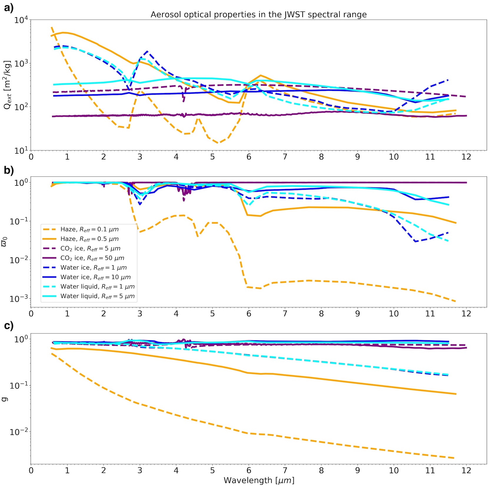
Figure 1: a) extinction cross section (Q_ext), single scattering albedo ($\varpi_{0}$) and asymmetry parameter of the phase function (g) as a function of the wavelength across JWST NIRSpec Prism and MIRI LRS ranges.

2.3.2 JWST instruments and noise

We estimate that NIRSpec Prism is the most instrument of JWST to characterize TRAPPIST-1 planets with transmission spectroscopy because it has a relatively wide wavelength coverage from 0.6 to 5.3 $\mu m$, for a resolving power (R) of 300 and TRAPPIST-1 should not reach the saturation of the detector. Note that partial saturation (in the SED peaks) strategy or alternate readout mode (Batalha et al., 2018) can yield considerably better results in terms of fewer transits required to reach a desired S/N on gas detections (Batalha et al., 2018; Lustig-Yaeger et al., 2019).

In addition, some interesting gaseous features for the Earth-like atmospheres (Archean and modern) such as the methane (CH₄) and ozone (O₃) absorption lines are also accessible in the JWST MIRI -resolution spectroscopy (LRS, R=100) with the wavelength range of $5.0-12.0\ \mu m$. In this work, spectra are showed with R=300 across NIRSpec and MIRI ranges to have continuous spectra from 0.6 to $20\ \mu m$ with a constant resolving power. However, to calculate S/N in MIRI range we use R=100 or below.

PSG includes a noise calculator to account for the following: the noise introduced by the source itself (N_source), the background noise (N_back) following a Poisson distribution with fluctuations depending on $\sqrt{N}$ with $N$ the mean number of photons received (Zmuidzinas, 2003), the noise of the detector (N_D) and the noise introduced by the telescope (N_optics). The total noise being then $N_{total}=\sqrt{N_{source}+N_{back}+N_{D}+N_{optics}}$.

3 Modern Earth-like atmospheres

3.1 Climate

when the question of a planet’s habitability arises, . With LMD-G we have considered a 1 bar atmosphere composed of N₂ and 376 ppm of CO₂. While modern Earth consists of $78\%$ of N₂ and $21\%$ of O₂ both gases have similar impacts on a planet’s climate so we only take into account N₂ for the GCM simulations. O₂ and other minor gases will be considered in the photochemistry computation with Atmos. The surface temperature and water cloud path ($kg\cdot m^{-2}$) for TRAPPIST-1e, f and g are shown in Fig. 2. TRAPPIST-1e is the only planet to have an ice-free surface around the substellar point and a thick cloud deck going up to the terminator (especially at high latitudes pushed by Rossby waves from the substellar point). Thick clouds ($>10^{-3}\ kg\cdot m^{-2})$ are present in the east terminator of TRAPPIST-1f but not in TRAPPIST-1g. Table 3 lists the mean, maximum and minimum surface temperature as well as the integrated column of condensed species for TRAPPIST-1e, f and g. We can see that both the surface temperatures and amount of condensed species are much lower for the modern Earth-like atmosphere than for the CO₂ dominated atmosphere at 1 bar surface pressure (see Table 7). The mean surface temperature of TRAPPIST-1e (244 K) is in very good agreement with 3-D climate simulations with CAM4 GCM Wolf (2017) (241 K) and LMD-G GCM Turbet et al. (2018) (248 K; 4 K difference arises due to the use of updated planetary parameters) but far from the 1-D simulation of Lincowski et al. (2018) (279 K and 282 K for the clear and cloudy simulations, respectively).

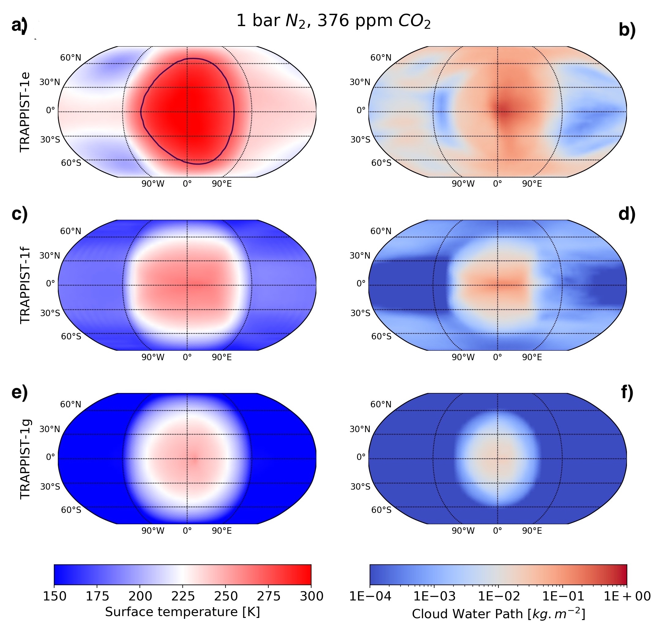
Figure 2: Surface temperature (left column) and cloud water path (right column) for TRAPPIST-1e (top row), 1f (middle row) and 1g (bottom row). The blue line shows the sea-ice boundary. Note, only TRAPPIST-1e has any ice-fee ocean.

Table 3: Surface temperatures (TS) and integrated column of condensed species for the modern Earth-like atmosphere. Values with an asterisk are averaged around the terminator only.

	Planets
TS mean [$K$]	244	197	168
TS min [$K$]	194	157	126
TS max [$K$]	304	266	256
H2O liq* [$10^{-3}kg\cdot m^{-2}$]	1.3	0.0	0.0
H2O ice* [$10^{-3}kg\cdot m^{-2}$]	13.6	$6.0\times 10^{-1}$	$1.3\times 10^{-2}$
CO2 ice* [$10^{-3}kg\cdot m^{-2}$]	0.0	0.0	0.0

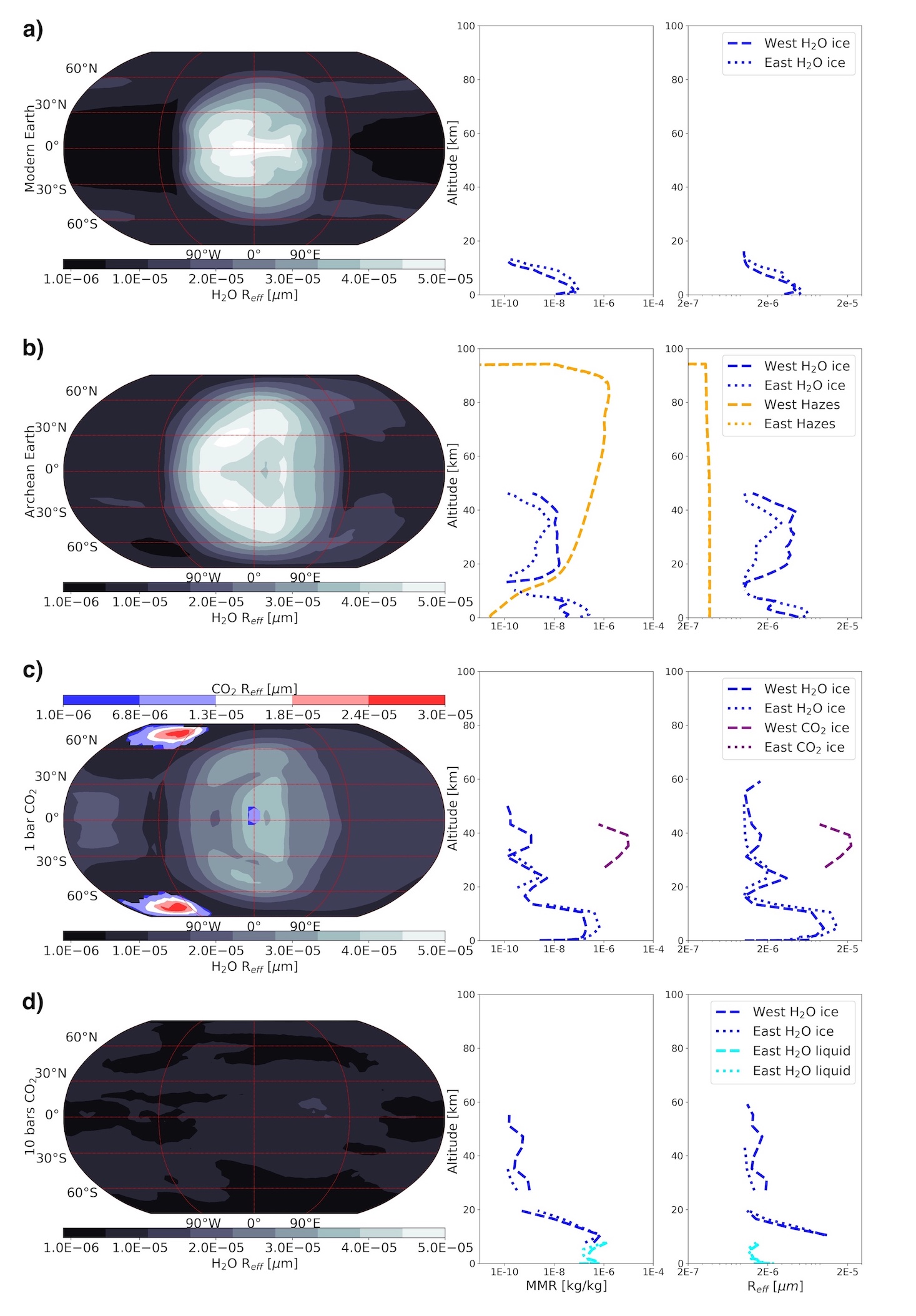
Figure 3: Left panel: vertically averaged cloud effective radius (R_eff), right panel: vertical distribution of the mass mixing ratio (MMR) and R_eff at the East and West terminator for various aerosols . Note that hazes are only generated with the Atmos photochemical model. When the MMR is very low, typically below $10^{-10}$ kg/kg, the R_eff is tiny and its dimension and optical properties are poorly constrained. LMD-G set up therefore the R${}_{eff}=10^{-6}\ \mu m$ threshold as the minimum value to be output. Therefore, MMR value below $10^{-10}$ kg/kg and R${}_{eff}\ \leq 10^{-6}\ \mu m$ have been excluded from the averaging.

To simulate more gases in the planet’s atmosphere than the ones used in the GCM climate module (N₂, CO₂, CH₄ and H₂O), we run the Atmos photochemical model at the terminator (ignoring feedback on the climate) from atmospheric profiles (temperature, pressure and mixing ratios) computed by LMD-G. Figure 4 shows a selection of averaged atmospheric profiles around the terminator for TRAPPIST-1e, 1f and 1g obtained with Atmos The atmospheric profiles presented here are then used, along with cloud profiles from LMD-G, to simulate the transmission spectra.

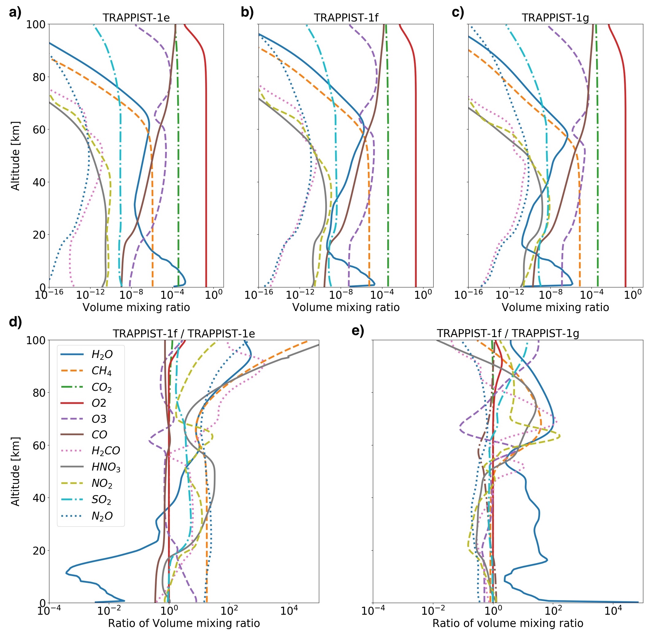
Figure 4: Gas mixing ratio profiles for TRAPPIST-1e, 1f and 1g, as well as profile ratios between TRAPPIST-1f and 1e and between TRAPPIST-1f and 1g .

3.2 JWST simulated spectra: Impact of H₂O clouds

The NIRSpec Prism and MIRI transmission spectra at R=300 for TRAPPIST-1e, f and g with the with boundary conditions based on the modern Earth are presented in Fig. 5. The relative transit depth, the signal-to-noise ratio for 1 transit (S/N-1) and the number of transits needed to achieve $3\ \sigma$ and a $5\ \sigma$ detections are summarized in Table 4 for selected absorption lines. A resolving power of R=30 has been adopted to optimize the S/N (Morley et al., 2017) while determining the number of transits.

The mathematical expression between the relative transit depth and the transit atmospheric thickness is (Winn, 2010):

$$\begin{split}\delta\Delta=(\delta R/R_{s})^{2}+(2\times R_{p}\times\delta R)/R_{s}^{2}\\ \sim(2\times R_{p}\times\delta R)/R_{s}^{2}\end{split}$$ (1)

with $\Delta$ and $\delta\Delta$ the transit depth and relative transit depth, respectively, in part-per-million, $R_{p}$ the planet’s radius, $\delta R$ the transit atmospheric thickness and $R_{s}$ the radius of the star in kilometer unit. Note that $(R_{p}/R_{s})^{2}$ represents the transit depth for an air-less planet. We can see that $\delta\Delta$ is dependent on the planet’s radius. The planetary radius is increasing from TRAPPIST-1e to -1f and -1g (see Table 1), transit depth for TRAPPIST-1g. Note that $\delta\Delta$ and $\delta R$ decrease with decreasing temperature or increasing gravity. Yet, TRAPPIST-1g is the coldest planet but also one with the lowest gravity.

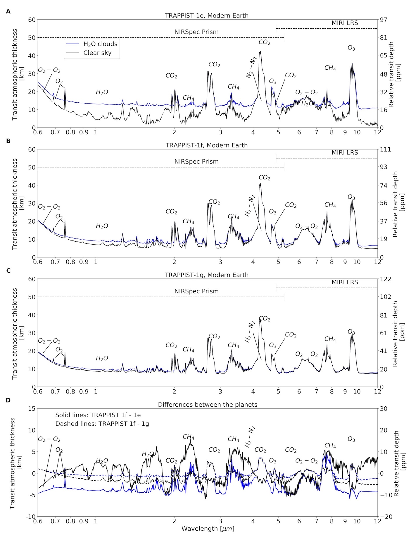
Figure 5: Simulated transmission spectra by JWST NIRSpec Prism and MIRI with R=300 for aquaplanets A) TRAPPIST-1e, B) 1f and C) 1g

Table 4: Relative transit depth (ppm), signal-to-noise ratio for 1 transit (S/N-1) and number of transits to achieve $5\ \sigma$ and $3\ \sigma$ detection for various spectral lines of the modern Earth-like atmosphere. Numbers in parentheses are for clear sky only while numbers without parentheses are the real values accounting for the impact of clouds. The hyphen represents the cases for which more than 100 integrated transits are needed

Planets
Instrument
Feature	O2 $0.8\ \mu m$
Depth [ppm]	5(10)	9(10)	10(11)
S/N-1	0.0(0.1)	0.1(0.1)	0.1(0.1)
N transits ($5\sigma$)	-(-)	-(-)	-(-)
N transits ($3\sigma$)	-(-)	-(-)	-(-)
Feature	H2O $1.4\ \mu m$
Depth [ppm]	2(10)	2(3)	3(3)
S/N-1	0.0(0.2)	0.1(0.1)	0.1(0.1)
N transits ($5\sigma$)	-(-)	-(-)	-(-)
N transits ($3\sigma$)	-(-)	-(-)	-(-)
Feature	CH4 $3.3\ \mu m$
Depth [ppm]	12(20)	24(27)	25(26)
S/N-1	0.2(0.5)	0.5(0.6)	0.5(0.7)
N transits ($5\sigma$)	-(-)	-(76*)	83*(74*)
N transits ($3\sigma$)	-(55)	36(27)	30(27)
Feature	CO2 $4.3\ \mu m$
Depth [ppm]	47(61)	60(63)	58(60)
S/N-1	0.8(1.1)	1.1(1.2)	1.2(1.2)
N transits ($5\sigma$)	35(21)	20(18)	19(18)
N transits ($3\sigma$)	13(8)	7(6)	7(6)
Instrument
Feature	$O_{2}-O_{2}$ $6.5\ \mu m$
Depth [ppm]	14(27)	22(26)	23(25)
S/N-1	0.1(0.2)	0.2(0.2)	0.2(0.2)
N transits ($5\sigma$)	-(-)	-(-)	-(-)
N transits ($3\sigma$)	-(-)	-(-)	-(-)
Feature	CH4 $7.7\ \mu m$
Depth [ppm]	13(24)	29(33)	31(32)
S/N-1	0.1(0.2)	0.2(0.2)	0.2(0.2)
N transits ($5\sigma$)	-(-)	-(-)	-(-)
N transits ($3\sigma$)	-(-)	-(-)	-(-)
Feature	O3 $9.6\ \mu m$
Depth [ppm]	36(48)	43(47)	44(46)
S/N-1	0.1(0.2)	0.2(0.3)	0.2(0.4)
N transits ($5\sigma$)	-(-)	-(-)	-(-)
N transits ($3\sigma$)	-(-)	-(-)	-(-)

We can see that H₂O clouds raise the continuum level up to a few kilometers above the surface, flattening the H₂O lines and reducing the relative transit depth (or atmospheric thickness) of other species. We have determined that the H₂O line at $1.14\ \mu m$ is the strongest H₂O line not being blended by CO₂ for such an atmosphere. Indeed, even the well-known $2.7\ \mu m$ H₂O line is completely dominated by CO₂ in this same spectral region, because H₂O is confined to the lower atmosphere where the opacity to the infrared radiation is high and where clouds are located. However, the relative transit depth of that H₂O line, or any other, is so low (only a few ppm) that it is very challenging to detect.

4 Archean Earth-like atmospheres

4.1 Climate

The climate of the Archean era (3.8-2.5 Ga) is still being debated. In this study we chose to use the three Archean Earth atmospheric compositions by Charnay et al. (2013) that were previously simulated with LMD-G. Those configurations for a 1 bar surface pressure are dominated by N₂ with the following amount of GHG:

• Charnay case A (900 ppm of CO₂, 900 ppm of CH₄)

• Charnay case B (10,000 ppm of CO₂, 2,000 ppm of CH₄)

• Charnay case C (100,000 ppm of CO₂, 2,000 ppm of CH₄)

The surface temperatures and the water cloud columns are displayed in Fig. 6 and Fig. 7, respectively. Mean, values are reported in Table 5.
Again, we were not able to find a stable climate state for TRAPPIST-1g with a Charnay case C atmosphere, because CO₂ condenses on the night side.
In Fig. 6 we can see that the surface temperature is increasing from Charnay case A to Charnay case C for TRAPPIST-1e while for TRAPPIST-1f and -1g, the surface temperature is maximum for Charnay case A, followed by case C and finally case B. On the one hand, for TRAPPIST-1e, the atmosphere is warm and moist and the water feedback has a large effect, as well as the change of albedo due to clouds and the ratio of water/ice surfaces; on the other hand for TRAPPIST-1f and -1g, their dryer atmosphere leads to a weak water feedback and the increase of CH₄ from Charnay Case A to Charnay case B promotes an anti-greenhouse effect, more powerful than the increase of CO₂. As a result, Charnay case B is the coolest. In Fig. 7 the relative amount of condensed water between the cases follows the surface temperature, with the largest cloud coverage for TRAPPIST-1e being Charnay case C, while for TRAPPIST-1f and -1g it is Charnay case A.

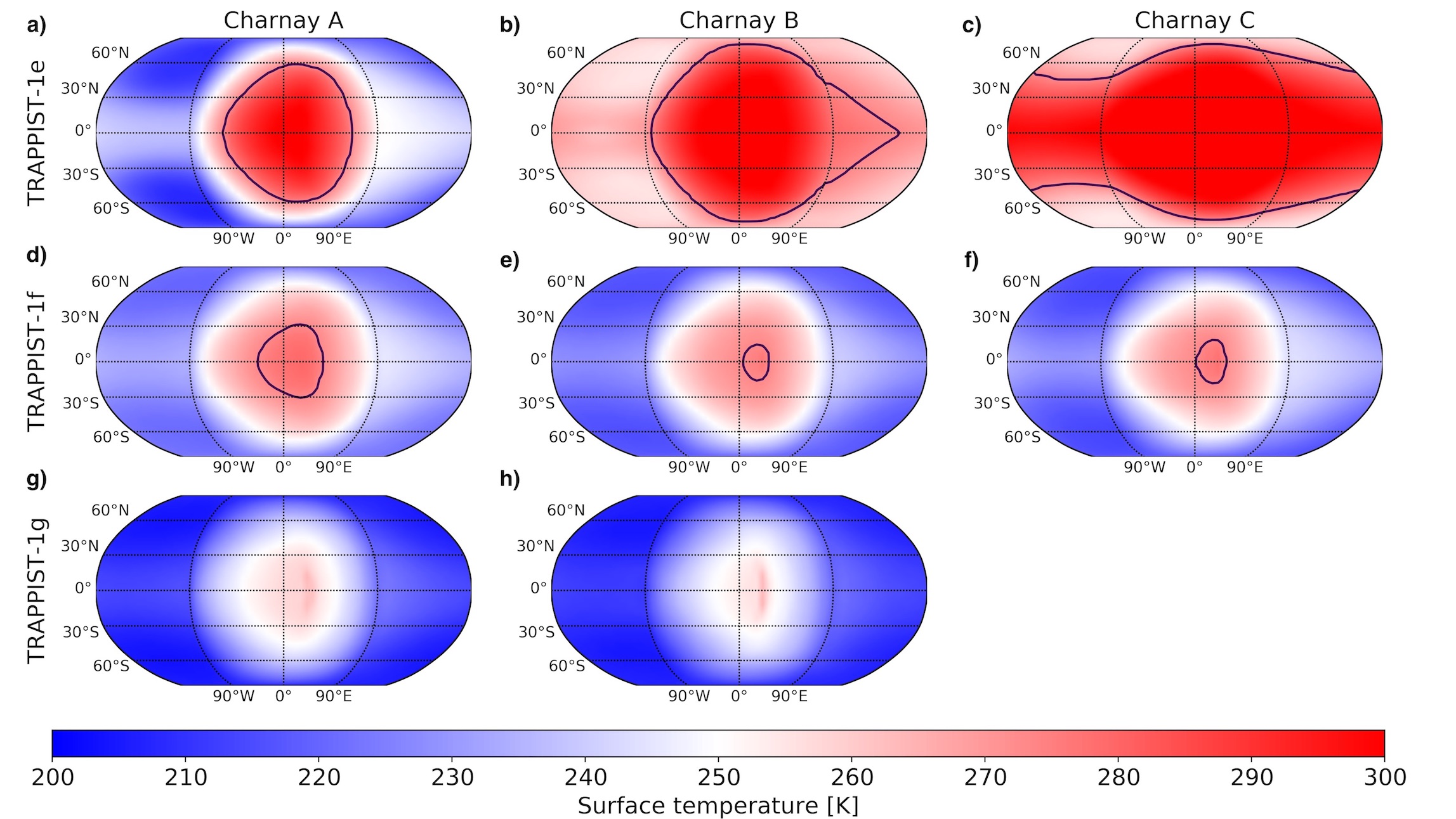
Figure 6: Surface temperature map in Kelvin (K) for aquaplanets TRAPPIST-1e (top row), TRAPPIST-1f (middle row) and TRAPPIST-1g (bottom row) for Charnay et al. (2013) case A (left), case B(middle) and case C (right) Archean Earth atmospheres. TRAPPIST-1g case C is missing because CO₂ in the atmosphere has condensed to the night side leading to the crash of the simulation. The blue line shows the sea-ice boundary.

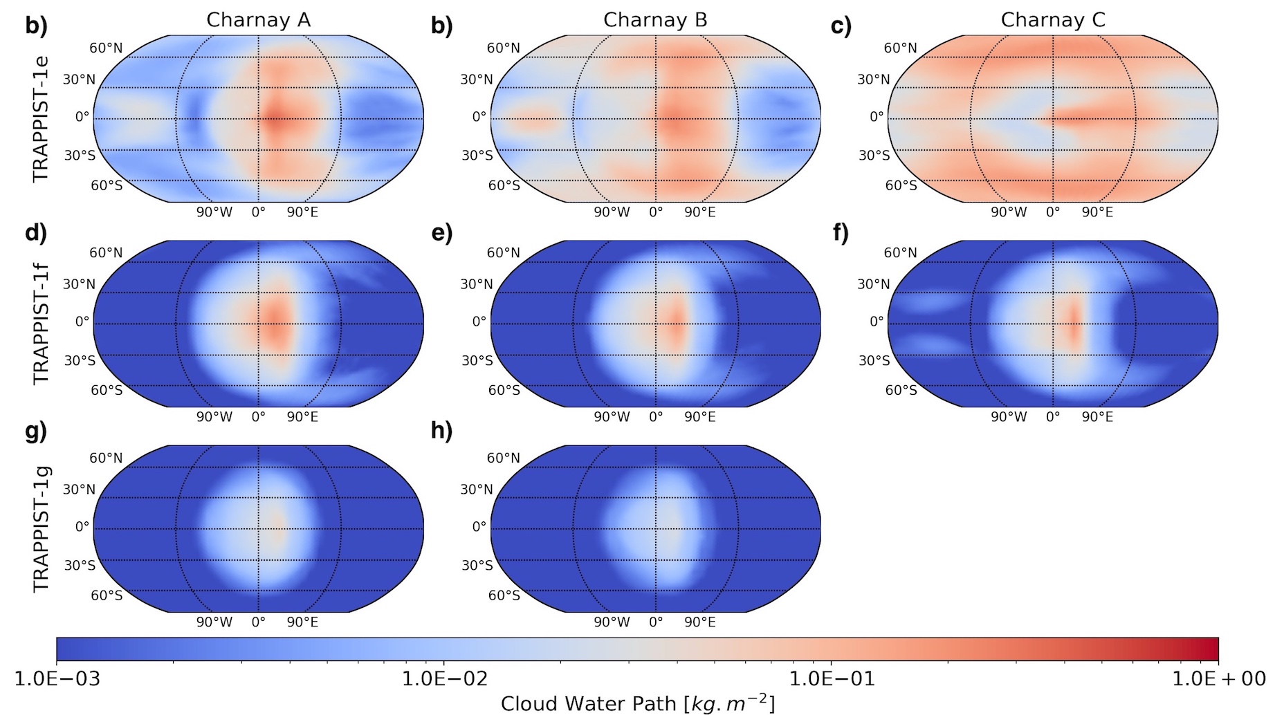
Figure 7: Integrated cloud water column in $kg.m^{-2}$ for aquaplanets TRAPPIST-1e (top row), 1f (middle row) and 1g (bottom row) for Charnay et al. (2013) case A (left), case B (middle) and case C (right) Archean Earth atmospheres. TRAPPIST-1g case C is missing because CO₂ in the atmosphere has condensed to the night side leading to the crash of the simulation.

Table 5: Surface temperatures (TS) and integrated column of condensed species for the Archean Earth-like atmosphere. Values with an asterisk are averaged around the terminator only.

	Planets
	A	B	C	A	B	C	A	B
TS mean [$K$]	243	273	286	238	234	235	204	221
TS min [$K$]	207	254	254	219	215	214	203	205
TS max [$K$]	305	310	324	279	277	278	204	264
H2O liq* [$10^{-3}kg\cdot m^{-2}$]	3.7	12.0	74.5	0.0	0.0	0.0	0.0	0.0
H2O ice* [$10^{-3}kg\cdot m^{-2}$]	12.6	24.7	26.1	1.1	0.81	0.93	0.07	0.05

For planets for which the ratio of methane over carbon dioxide (CH₄/CO₂) in the atmosphere exceeds about 0.1, haze formation can occur (Arney et al., 2016). Such hydrocarbon haze is generated by methane photolysis from $Ly\ \alpha$. Only Charnay Case A and B have the required CH₄/CO₂ to produce photochemical hazes. For this study, we have performed the photochemistry and transmission spectra simulations only for Charnay case B. This case offers larger concentrations of CO₂ and CH₄ than Charnay case A and can produce photochemical hazes contrary to Charnay case C. The Charnay case B Archean Earth-like atmospheric profiles is shown in Fig. 8.

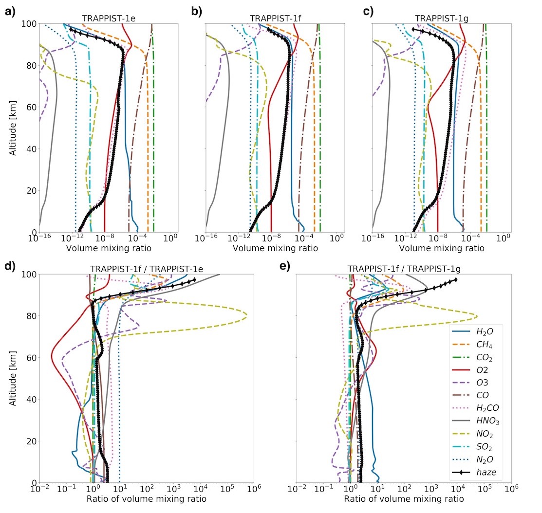
Figure 8: Gas mixing ratio profiles for an Archean Earth-like composition of Charnay et al. (2013) case B for TRAPPIST-1e, 1f and 1g, as well as profile ratios between TRAPPIST-1f and 1e and between TRAPPIST-1f and 1g.

4.2 JWST simulated spectra: Impact of H₂O clouds and photochemical hazes

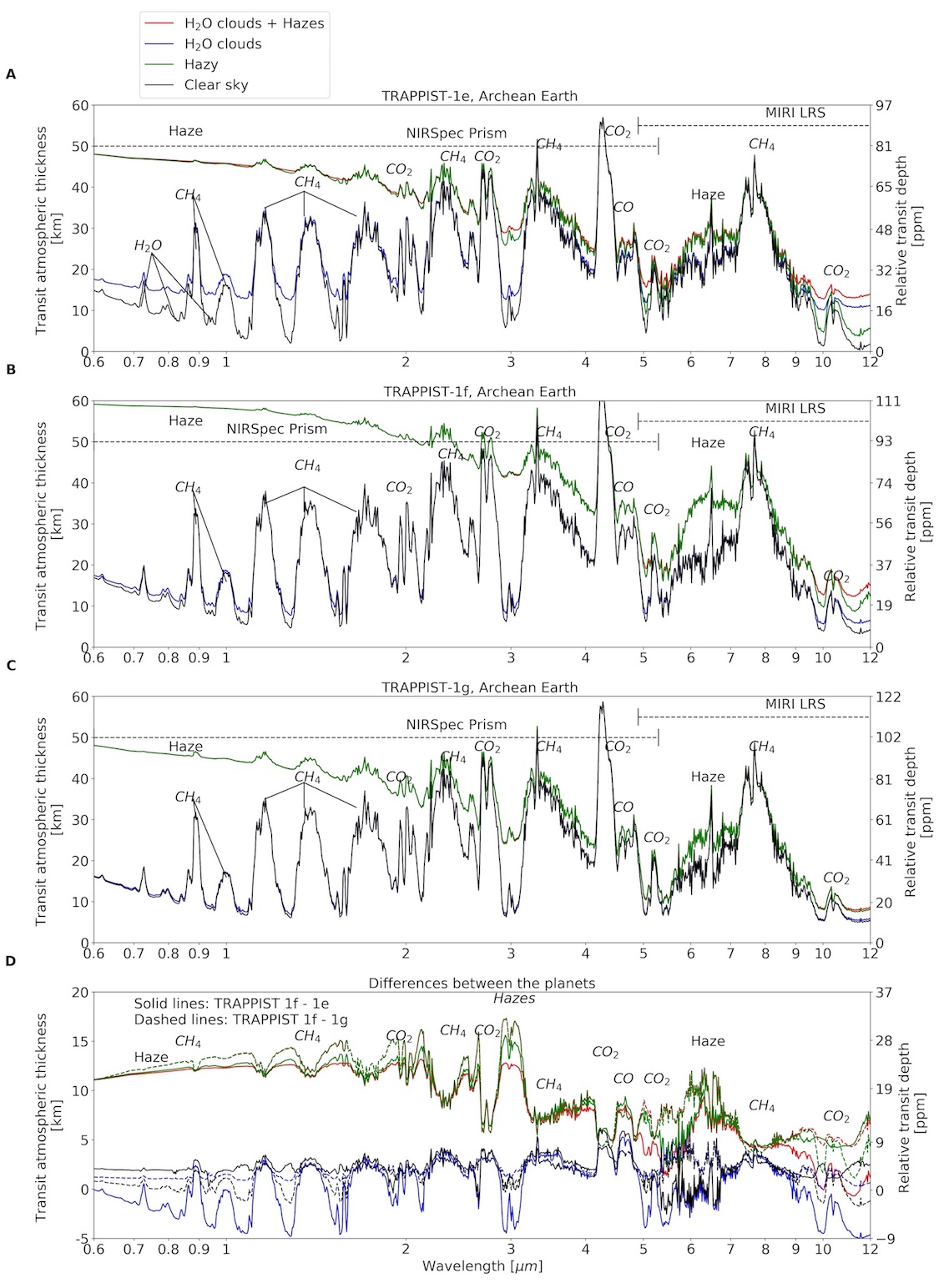
Figure 9: Simulated transmission spectra by JWST NIRSpec Prism and MIRI with R=300 for aquaplanets A) TRAPPIST-1e, B) 1f and C) 1g with the Archean Earth atmosphere composition of Charnay et al. (2013) case B. Panel D) shows differences between planetary spectra.

Table 6: Relative transit depth (ppm), signal-to-noise ratio for 1 transit (S/N-1) and number of transits to achieve a $5\ \sigma$ and $3\ \sigma$ detection for various spectral lines of the Archean Earth-like atmosphere of Charnay case B. Numbers in parentheses are for clear sky only while numbers without parentheses are the real values accounting for the impact of clouds and hazes. The hyphen represents the cases for which more than 100 integrated transits are needed .

Planets
Instrument
Feature	CH4 $1.2\ \mu m$
Depth [ppm]	2(44)	1(55)	4(56)
S/N-1	0.1(1.0)	0.1(1.4)	0.1(1.5)
N transits ($5\sigma$)	-(23)	-(13)	-(12)
N transits ($3\sigma$)	-(8)	-(5)	-(4)
Feature	CO2 $4.3\ \mu m$
Depth [ppm]	59(85)	72(108)	86(111)
S/N-1	1.1(1.6)	1.4(2.2)	1.7(2.3)
N transits ($5\sigma$)	23(9)	14(5)	9(5)
N transits ($3\sigma$)	8(3)	5(2)	3(2)
Feature	CO $4.7\ \mu m$
Depth [ppm]	4(39)	8(54)	8(53)
S/N-1	0.1(0.7)	0.1(1.0)	0.1(1.0)
N transits ($5\sigma$)	-(59)	-(27)	-(25)
N transits ($3\sigma$)	-(21)	-(10)	76*(9)
Instrument
Feature	CH4 $7.7\ \mu m$
Depth [ppm]	44(66)	60(82)	67(86)
S/N-1	0.3(0.6)	0.4(0.8)	0.5(0.8)
N transits ($5\sigma$)	-(80)	-(44)	98*(36)
N transits ($3\sigma$)	-(29)	52(16)	35(13)

Figure 9 shows the TRAPPIST-1e, 1f and 1g transmission spectra, for Charnay case B Archean Earth atmosphere with JWST NIRspec Prism and MIRI LRS. The hazes have a huge opacity down to the VIS/NIR which flattens most of the spectral features in the NIRSpec Prism range.
In the MIRI range, the hazes are clearly visible between 6 to $7\ \mu m$ opacity progressively decreases (see Fig. 1) and clouds become the largest source of opacity in the spectrum for TRAPPIST-1e and 1g (haze opacity in TRAPPIST-1f dominates the cloud opacity across the whole wavelength range). The combined impact of clouds and hazes in the detectability of gaseous features is summarized in Table 6. TRAPPIST-1g is the coldest and most distant of the three planets. has the smallest amount of clouds and hazes allowing for less transits to detect the spectral lines than for the two other planets The most favorable band CO₂ is at $4.3\ \mu m$ despite the presence of hazes at this wavelength, with only about 23, 14 and 9 transits required for a $5\ \sigma$ detection. The strength of the nearby CO feature is too weak to be detectable because of the continuum raised by hazes but also because, as mentioned previously, CO abundances may have been underestimated by fixing modern Earth mixing ratio and not predicting CO fluxes. H₂O lines are either too shallow or are blended by CH₄ or CO₂ that they are undetectable.

5 CO₂ atmospheres

5.1 Climate

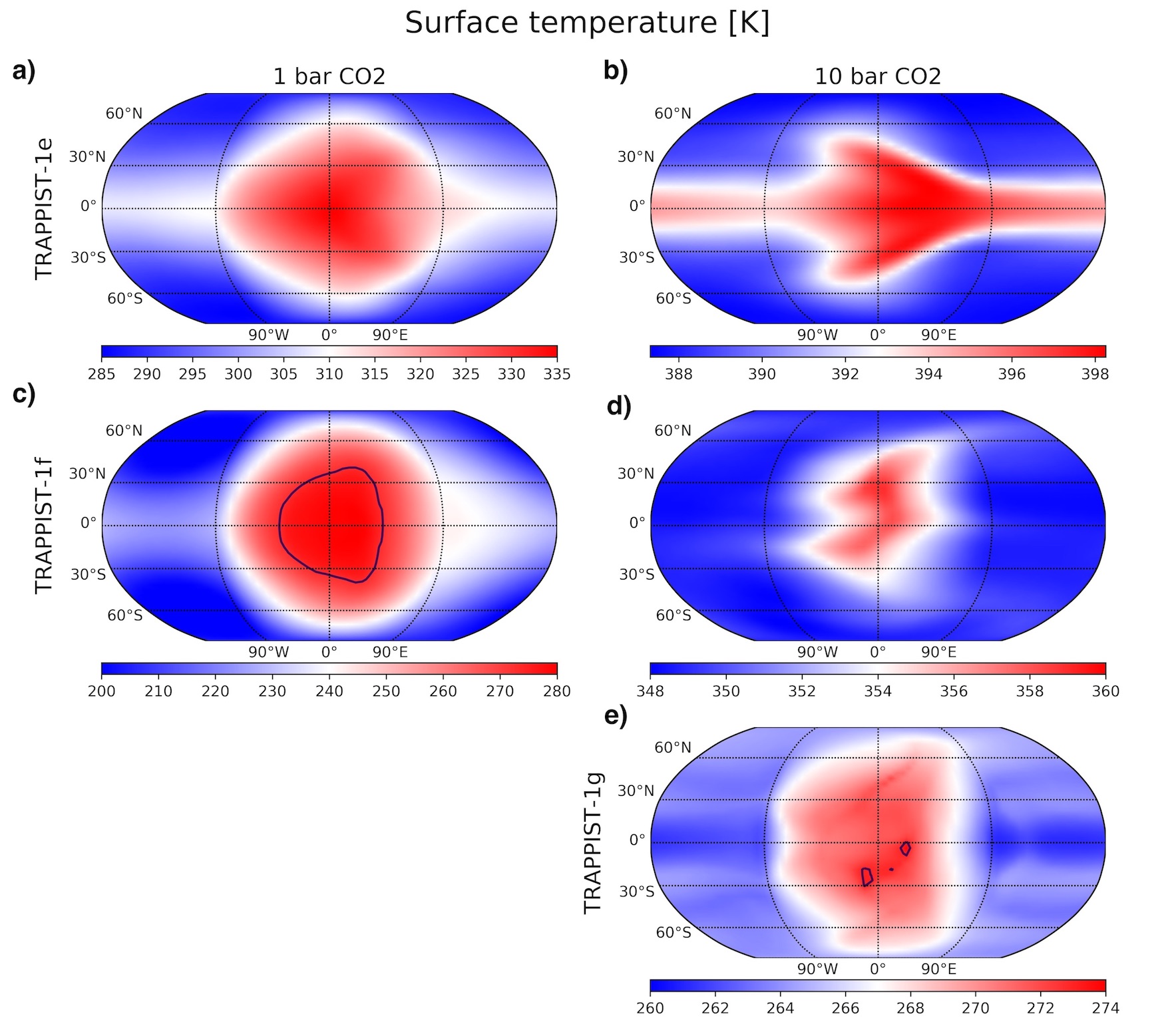
Figure 10: Surface temperature map in Kelvin (K) for aquaplanets TRAPPIST-1e (top row), TRAPPIST-1f (middle row) and TRAPPIST-1g (bottom row) at 1 (left column) and 10 (right column) bar of CO₂ surface pressure. TRAPPIST-1g at 1 bar is missing because the atmosphere would collapse on the night side. Note that the temperature scale is different for each of the subplot in order to highlight the so-called ”lobster pattern” of TRAPPIST-1e at 10 bars which has a thermal amplitude of only 10 K. The blue line shows the sea-ice boundary. Note that TRAPPIST-1e at 1 and 10 bars are completely ice-free.

Among the four rocky planets of our solar system, CO₂ is the dominant gas on two of them (Venus and Mars), and is thought to have been a dominant gas in early Earth’s atmosphere, in particular during the Hadean epoch (Zahnle et al., 2010). Therefore, it is reasonable to think that CO₂ atmospheres may be common in other planetary systems as well. de Wit et al. (2018); Moran et al. (2018) have shown that if the TRAPPIST-1 planets have an atmosphere, they should be free of low mean-molecular weight gases such as hydrogen or helium in absence of haze. This raises a possibility of high mean molecular weight species, such as CO₂, as a possible constituent. For each planet in the habitable zone of TRAPPIST-1 (i.e. planet e, f and g), we used LMD-G to simulate CO₂-dominated atmospheres with 1 and 10 bar surface pressures. However, we were not able to successfully simulate the 1 bar CO₂ atmosphere for TRAPPIST-g, because the atmospheric temperature on the night side is cold enough that CO₂ condenses on the surface, resulting in atmospheric collapse. TRAPPIST-1g retaining 1 bar or less of CO₂ is therefore highly unstable and unlikely to Turbet et al. (2018). Figure 10 shows the surface temperature maps, averaged over 10 orbits, of 1 bar (left column) and 10 bars (right column) CO₂-dominated atmospheres for TRAPPIST-1e (top row), f (middle row) and g (bottom row). Surface temperatures and integrated columns of condensed species are reported in Table 7. As for the modern Earth-like atmosphere, mean surface temperatures predicted by the GCM for the 10 bars cases agree with other GCM simulations (Wolf, 2017) but are much higher than the one predicted with 1-D climate model of Lincowski et al. (2018) for their 10 bars Venus -like atmospheres primarily due to the cooling of the highly reflective sulfuric acid aerosols (not included in Wolf (2017) nor in our study). Note that none of the 10 bars simulations are cold enough to have CO₂ condensation at the surface (below 233.6 K), in agreement with Turbet et al. (2018). At 1 bar, we can see that TRAPPIST-1e is ice-free, while TRAPPIST-1f is an ”eye-ball” planet, with an open ocean restricted to the substellar region, roughly between -40 and +40 longitude East and -40 and +40 latitude North. In both cases, the surface temperature contrast between the substellar and anti-substellar region is roughly 100 K. At 10 bar surface pressure, the atmosphere is very efficient to transport the heat and the contrast is only on the order of 10 K for TRAPPIST-1e, f and g. Very interestingly, because of the faster rotation period of TRAPPIST-1e (6.1 days) a so-called ”lobster pattern” appears, which is usually seen when a dynamic ocean is coupled to the atmosphere (Hu & Yang, 2014; Del Genio et al., 2019). This asymmetric pattern of surface temperature is due the combination of a Rossby wave, West to the substellar point, moving the warm air away from the equator, and a Kelvin wave, East of the substellar point, progressing exclusively in the longitude-altitude plane. While ocean heat transport is not included in our simulation, the combination of the dense atmosphere and fast rotation rate are responsible for this pattern.

Table 7: Surface temperatures (TS) and integrated column of condensed species for the CO₂ dominated atmospheres. Values with an asterisk are averaged around the terminator only.

Planet
	CO2 dominated		CO2 dominated		CO2 dominated
Pressure	1 bar	10 bar	1 bar	10 bar	10 bar
TS mean [$K$]	303	392	230	350	266
TS min [$K$]	285	387	194	348	261
TS max [$K$]	335	398	281	359	274
H2O liq* [$10^{-3}kg\cdot m^{-2}$]	61.3	28.3	$1.0\times 10^{-2}$	26.7	$2.0\times 10^{-1}$
H2O ice* [$10^{-3}kg\cdot m^{-2}$]	9.9	12.4	4.3	9.4	5.7
CO2 ice* [$10^{-3}kg\cdot m^{-2}$]	0.0	0.0	$3.1\times 10^{-2}$	$6.6\times 10^{-1}$	90.0

Figure 11 shows the integrated columns of H₂O condensates (liquid and ice). The largest cloud coverage was recorded for both TRAPPIST-1e and -1f at 1 bar, with a large cloud deck due to the strong convection and shifted eastward of the substellar point (Kopparapu et al., 2017; Yang et al., 2014) for TRAPPIST-1e due to the fast rotation. Note that for TRAPPIST-1f, the rotation is slower and the cloud deck is more centered toward the ice-free substellar region.
At 10 bar surface pressure, TRAPPIST-1e and -1f are so warm that the huge amount of water vapor brought to the atmosphere leads both inefficient radiative cooling and strong solar absorption in the low atmosphere, causing a net radiative heating of the layers near the surface; subsequently, this radiative heating creates a strong temperature inversion encompassing the entire planet, stabilizing the low atmosphere against convection, including at the substellar point (Wolf & Toon, 2015). Indeed, inversion layers are intrinsically stable against vertical mixing; without a deep convection carrying moisture up from the boundary layer, no substellar cloud deck is formed, and instead, the skies are relatively clear despite the enormous amount of water vapor in the atmosphere. TRAPPIST-1g is much colder, almost fully ice-covered except at a few spots near the substellar region (see Fig. 10 bottom row) where some water can evaporate from the ocean and form relatively thin clouds with a H₂O water cloud column of about 0.1 $kg\cdot m^{-2}$.

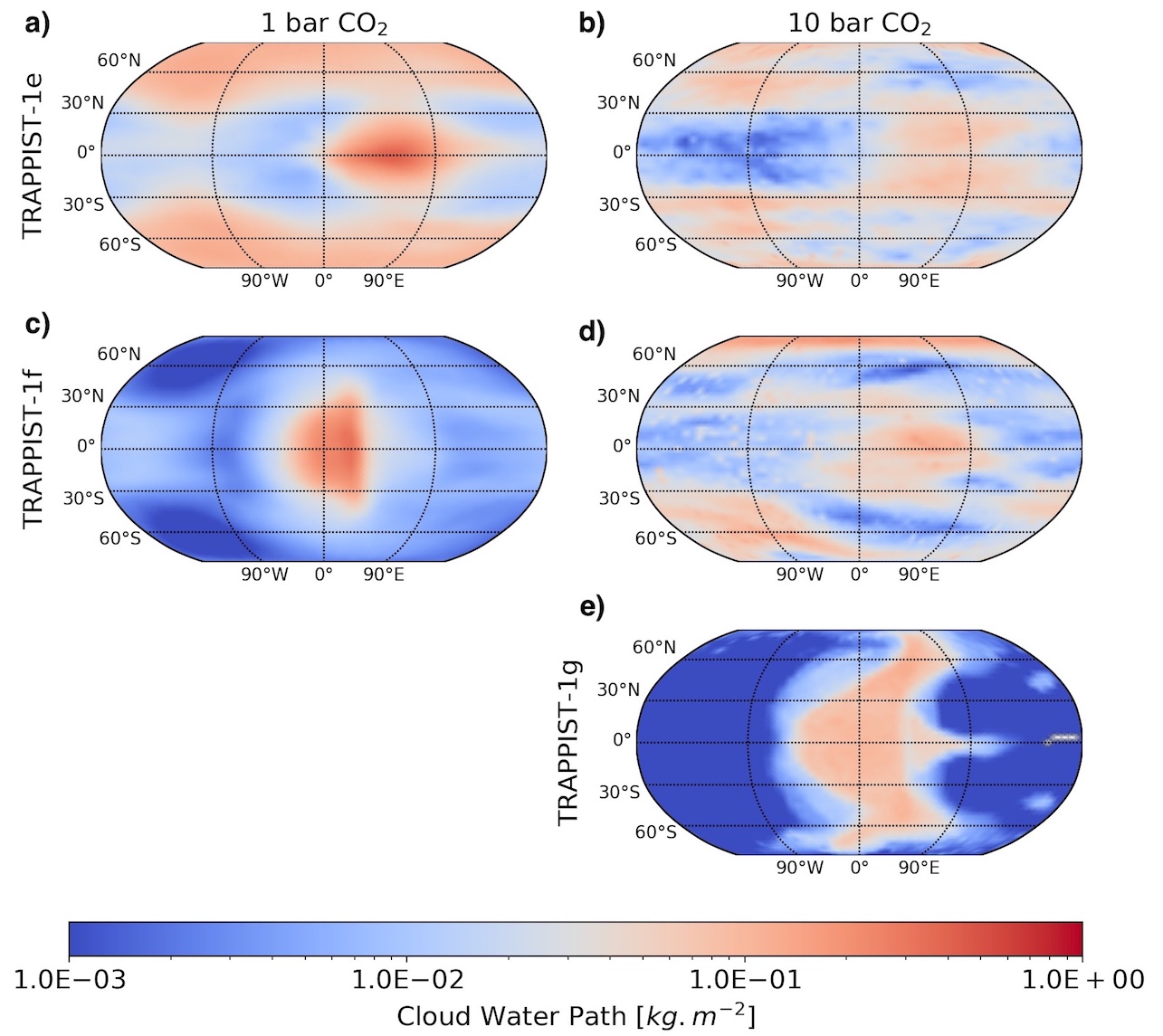
Figure 11: Integrated H₂O column in $kg.m^{-2}$ for aquaplanets TRAPPIST-1e (top row), TRAPPIST-1f (middle row) and TRAPPIST-1g (bottom row) at 1 (left column) and 10 (right column) bar of CO₂ surface pressure. TRAPPIST-1g at 1 bar is missing because the atmosphere has condensed to the night side leading to the crash of the simulation.

Figure 12 shows the integrated column of CO₂ ice. TRAPPIST-1e is too warm at 1 and 10 bars to have significant CO₂ condensation in the atmosphere. For TRAPPIST-1f, CO₂ starts to condense in two cold traps (Leconte et al., 2013b) at 1 bar at a symmetric position around longitude $-120^{\circ}$ and latitudes $\pm 80^{\circ}$ and between 30 and 50 km (see Fig.3) but their position can slightly vary, due to planetary-scale equatorial Kelvin and Rossby wave interactions (Showman & Polvani, 2011). Also, we notice that for a thicker atmosphere (10 bar) these two colds traps tend to move westward and toward highest latitudes and two others are at longitude $+150^{\circ}$ and latitudes $\pm 90^{\circ}$. Note that a few spots of CO₂ condensate appear eastward of (TRAPPIST-1e) and at (TRAPPIST-1f) the substellar point. This is due to a local temperature minimum at p=67 mbar near the substellar point marking the top of the ascending circulation branch (Carone et al., 2014, 2015, 2018). These CO₂ clouds near the substellar point would likely disappear due to the shortwave absorption of the CO₂ ice crystals but the radiative effect of CO₂ is not taken into account in our simulations.

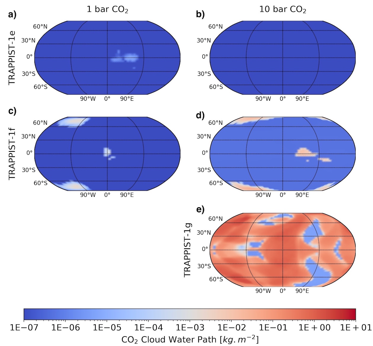
Figure 12: Integrated CO₂ column in $kg.m^{-2}$ for aquaplanets TRAPPIST-1e (top row), TRAPPIST-1f (middle row) and TRAPPIST-1g (bottom row) at 1 (left column) and 10 (right column) bar of CO₂ surface pressure. TRAPPIST-1g at 1 bar is missing because the atmosphere has condensed to the night side leading to the crash of the simulation. All planets are aquaplanets.

5.2 JWST simulated spectra: Impact of H₂O and CO₂ clouds

Figures 13 and 14 show JWST NIRSpec Prism and MIRI simulated transmission spectra for TRAPPIST-1e, 1f and -1g at 1 and 10 bar CO₂ surface pressures, respectively. In addition, The relative transit depth, the signal-to-noise ratio (S/N) for 10 transits and the number of transits for a $5\ \sigma$ and $3\ \sigma$ detection are reported in Table 8.

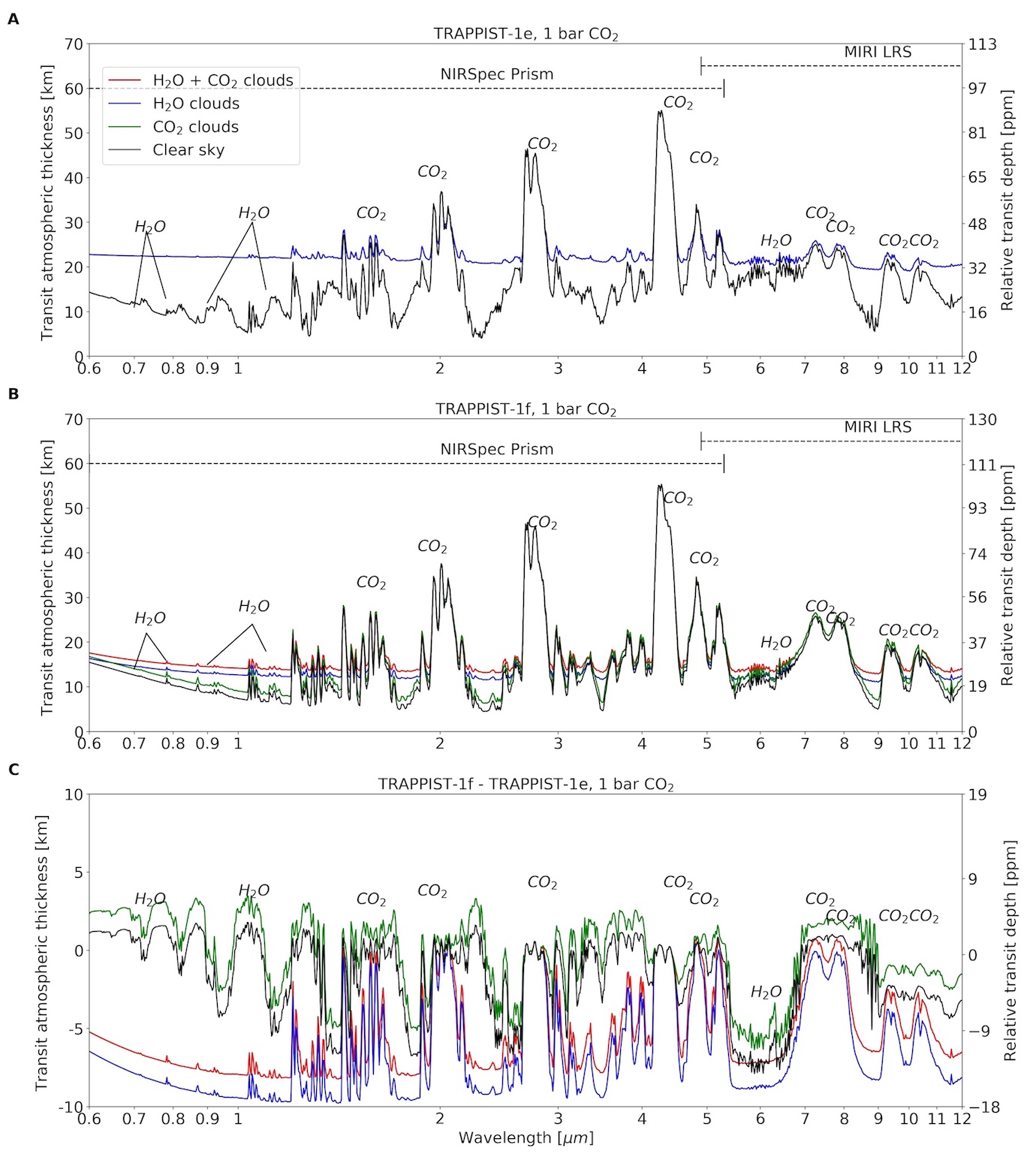
Figure 13: Simulated transmission spectra by JWST NIRSpec Prism and MIRI with R=300 for aquaplanets A) TRAPPIST-1e and B) 1f with 1 bar of surface pressure of CO₂. Panel D) shows differences between planetary spectra.

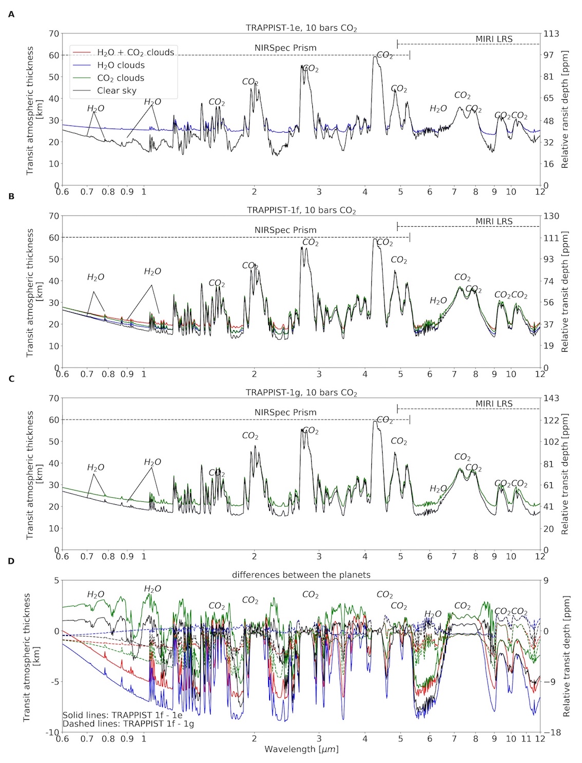
Figure 14: Simulated transmission spectra by JWST NIRSpec Prism and MIRI with R=300 for aquaplanets A) TRAPPIST-1e, B) 1f and C) 1g with 10 bars of surface pressure of CO₂. Panel D) shows differences between planetary spectra.

First, we can see that water clouds produce a considerable flattening of the spectra of TRAPPIST-1e, suppressing H₂O lines and leading to a continuum level at about 22 km in the 1 bar case. Around the terminator, the average liquid and ice water contents (LWC and IWC, respectively) are equal to $4.1\times 10^{-6}$ and $6.5\times 10^{-7}$ $kg\cdot m^{-3}$ for TRAPPIST-1e and 1f, respectively (see Table 7).

At 10 bar surface pressure, the mean surface temperature of TRAPPIST-1e is very high, 392 K, . At this temperature, the continuum of water vapor in the low atmosphere is opaque to the infrared radiation, and the continuum is pushed toward higher altitudes, even in clear sky, up to about 15 km. Figure 14 shows that this results in a reduction of the relative transit depth of every gas including CO₂

Similarly to the atmospheres with modern Earth and Archean Earth boundary conditions, we can see that H₂O lines are not detectable at $3\ \sigma$ or $5\ \sigma$ in less than 100 transits for the cloudy scenario. MIRI does not performed better, with no detectable H₂O lines. On the contrary, the well-mixed CO₂ is barely affected by the presence of clouds in the line region, because enough of it remains above the cloud deck. Because the continuum level is raised by the presence of clouds, the transit atmospheric thickness and transit depth of CO₂ is also reduced. CO₂ at 4.3 $\ \mu m$ has a transit depth of the order of 50 to 80 ppm and could be detected with NIRSpec from 10 to 30 transits at $5\ \sigma$ confidence level. Note that the number of transit at $5\ \sigma$ for the 10 bar clear sky case of TRAPPIST-1e (22) is the same as the one estimated by Lustig-Yaeger et al. (2019) for NIRSpec Prism sub512 mode.

Figure 15: Difference between the spectra of the 10 bars and 1 bar CO₂ surface pressure for aquaplanets A) TRAPPIST-1e and B) 1f.

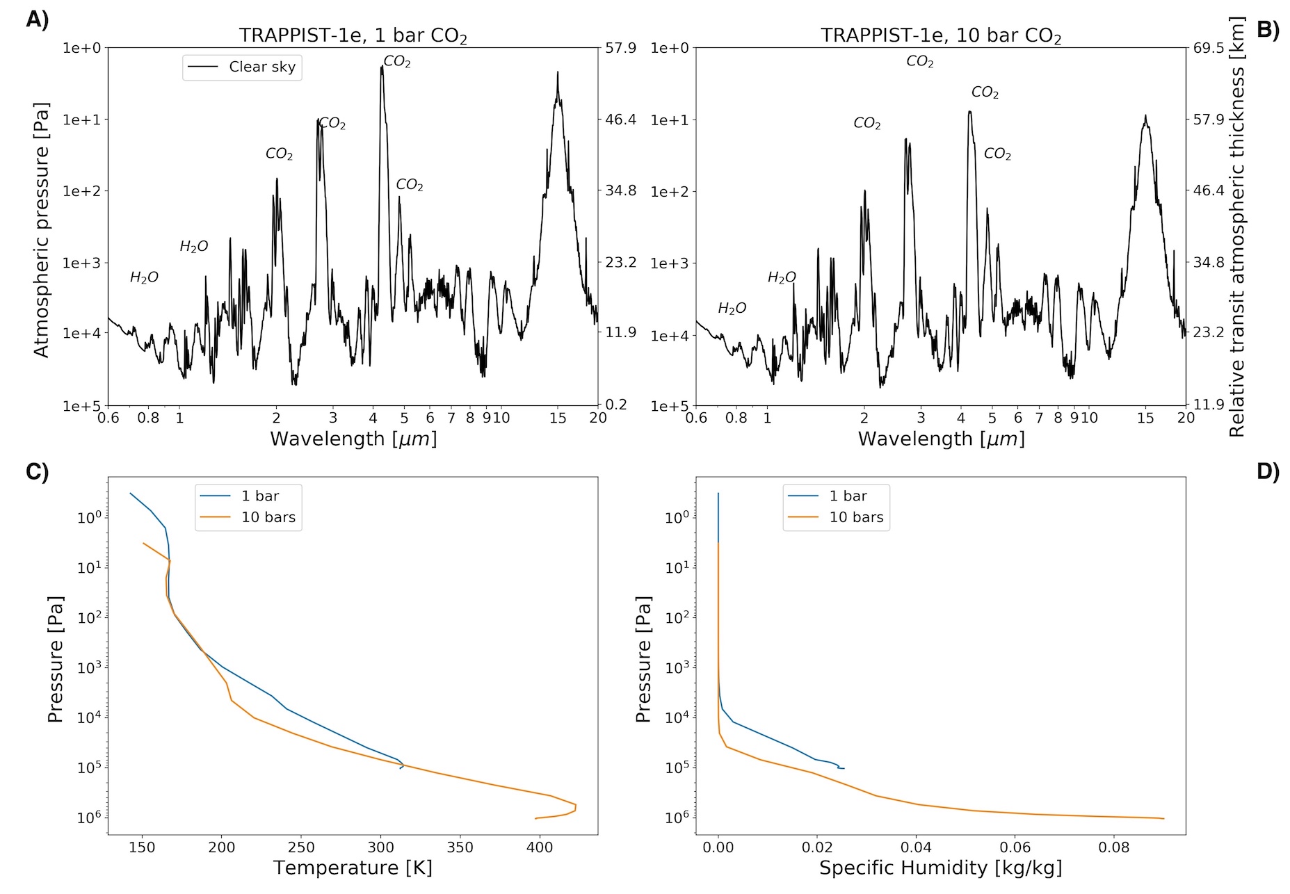
Figure 16: Simulated transmission spectra by JWST NIRSpec Prism and MIRI with R=300 for the aquaplanet TRAPPIST-1e with A) 1 bar and B) 10 bars of CO₂ surface pressure. C) Atmospheric temperature and D) specific humidity, averaged at the terminator, as a function of the atmospheric pressure for 1 and 10 bars CO₂ surface pressures.

Table 8: Relative transit depth (ppm), signal-to-noise ratio for 1 transit (S/N-1) and number of transits to achieve a $5\ \sigma$ and $3\ \sigma$ detection for various spectral lines of the CO₂ -dominated atmosphere. Numbers in parentheses are for clear sky only while numbers without parentheses are the real values accounting for the impact of clouds. The hyphen represents the cases for which more than 100 integrated transits are needed and the * mark denotes the values above the maximum number of transits observable per planet during JWST nominal lifetime mentioned in Table 1.

Planets
Pressures	1 bar	10 bar	1 bar	10 bar	10 bar
Feature	H2O $1.4\ \mu m$
Depth [ppm]	3(18)	3(14)	4(12)	5(9)	5(10)
S/N-1	0.1(0.4)	0.1(0.3)	0.1(0.3)	0.1(0.2)	0.1(0.2)
N transits ($5\sigma$)	-(-)	-(-)	-(-)	-(-)	-(-)
N transits ($3\sigma$)	-(54)	-(82)	-(-)	-(82*)	-(-)
Feature	CO2 $4.3\ \mu m$
Depth [ppm]	61(86)	50(56)	80(96)	60(66)	67(74)
S/N-1	1.2(1.6)	0.9(1.1)	1.6(1.9)	1.2(1.3)	1.4(1.6)
N transits ($5\sigma$)	19(9)	28(22)	10(7)	17(15)	13(10)
N transits ($3\sigma$)	7(3)	10(8)	4(2)	6(5)	5(4)

6 Discussion

6.1 Noise and detectability

In this section, we discuss the different noise sources that can impact JWST observations and the detectability of an atmosphere and/or of any gaseous feature.
The large aperture of JWST (6.5 m) will allow us to quickly acquire a significant number of photons after a few transits while the noise from the source (N_source) will largely dominate the total noise (N_total). every instrument suffers from a background red noise (of low frequency) which is a measurement error in addition to the frequency coming from the white noise (photon, reading, dark, etc). This red noise comes mainly from the systematic effects that affect the measurements, e.g., the fact that the pixels are not perfectly homogeneous (intra-pixel gain variability (Knutson et al., 2008; Anderson et al., 2011) and that the telescope does not track perfectly, resulting in a position-dependent low frequency noise which can be modeled but (because the model is never a perfect representation of the noise, and its parameters have their

According to Greene et al. (2016), instrumental noise (introduced by decorrelation residuals) produces systematic noise floors that do not decrease when acquiring more photons (with a larger aperture and/or more integration time), . In HST WFC3 observations of GJ 1214 Kreidberg et al. (2014), the errors obtained from integrated 15 transits are however in perfect agreement with a modeled ”pure white noise”, indicating a low noise (30 ppm) and decay close to . Tsiaras et al. (2016) report the most precise transmission spectrum for a planet (55 Cancri e) with a single visit with HST WFC3 reaching 20-30 ppm precision over 25 channels. In the infrared with the Spitzer space telescope, values as low as 65 ppm have been achieved (Knutson et al., 2009). If we observe a large number of transits, the difference in frequency between the systematic effects and the orbit of the planet will approach the reduction in of the white noise, but without ever reaching it . To suppose a fixed background (red) noise as in Greene et al. (2016) implies to neglect this decrease. However, the fact that a noise floor better than 30 ppm has not been achieved yet is not due to the precision limit of instruments like HST WFC3, but instead to the fact that no one has ever accumulated enough high S/N transits. Yet, it is only by accumulating a large number of transits of the same object with JWST that we will know if the instruments can do better, and measure the value of their background noise and the profile of its decay as a function of the number of transits. Note that this decay is very poorly characterized in IR spectrophotometry because to quantify it requires high S/N observations and many transits observed.
Another way to estimate what we can expect to achieve as estimated precision with JWST is to look at the accuracy reached by Spitzer or WFC3 at very high S/N, in photometry rather than in spectrophotometry. For HD 219134, Gillon et al. (2017b) have obtained a 20 ppm noise with only 2 transits at $4.5\ \mu m$, with a much less homogeneous InSb detector than the NIRSpec or WFC3 HgCdTe detector. Compared to the expected white noise, this produces a red noise of less than 10 ppm, despite systematics of about 1000 ppm amplitude.

Figure 17 shows the S/N (left Y-axis) and noise (right Y-axis) for the CO₂ line at 4.3 $\mu m$ of the modern Earth-like simulation as a function of the number of transits.

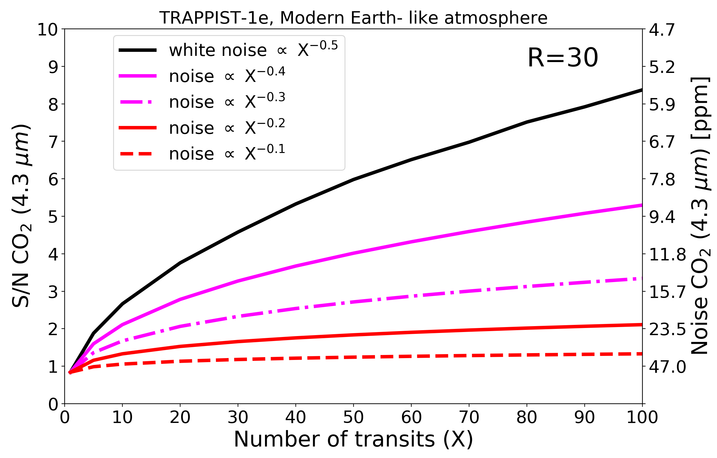
Figure 17: Signal-to-noise ration (S/N) (left y axis) and noise (right y axis) for the CO₂ line at 4.3 $\mu m$ of the modern Earth-like atmosphere simulated for JWST NIRSpec prism at R=30 as a function of the number of transits.

Meanwhile, in this study we consider the significance of a detection of an atmosphere (whatever the gas) at a $3\ \sigma$ confidence level but the detection of a specific biosignature gas such as O₂, O₃, CH₄ or even H₂O at $5\ \sigma$. The a priori noise floors should therefore be scaled accordingly by the factor of the confidence level. Table 9 shows the various noise floors as a function of the significant level considering either 20 and 50 ppm or 10 and 25 ppm, for NIRSpec and MIRI, respectively.

Table 9: A priori noise floors as a function of the detection confidence level from the conservative and optimistic $1\ \sigma$ noise floor estimations (first and second column, respectively, for each confidence level).

	$1\ \sigma$		$3\ \sigma$		$5\ \sigma$
NIRSpec prism	10	20	30	60	50	100
MIRI LRS	25	50	75	150	125	250

Table 4 (modern Earth atmosphere), Table 6 (Archean Earth atmosphere) and Table 8 (CO₂ rich atmospheres) If we assume the optimistic noise floors of Table 9, we estimate that an atmosphere can be detected by JWST using the CO₂ absorption at $4.3\ \mu m$ for:

• A modern Earth-like atmosphere with NIRSpec prism from 7 (TRAPPIST-1g) to 13 (TRAPPIST-1e ) transits at $3\ \sigma$ or 19 to 35 transits at $5\ \sigma$.

• An Archean Earth-like atmosphere with NIRSpec prism from 3 (TRAPPIST-1g) to 8 (TRAPPIST-1e) transits at $3\ \sigma$ or 9 (TRAPPIST-1g) to 23 (TRAPPIST-1e) transits at $5\ \sigma$.

• A CO₂ rich atmosphere (1 and 10 bars) with NIRSpec prism from 5 (TRAPPIST-1g) to 10 (TRAPPIST-1e) transits at $3\ \sigma$ or between 13 (TRAPPIST-1g) to 28 (TRAPPIST-1e) transits at $5\ \sigma$.

Considering the conservative noise floors (Greene et al., 2016) we estimate that an atmosphere can be detected (only at $3\ \sigma$) using the CO₂ absorption at $4.3\ \mu m$ for:

• A modern Earth-like atmosphere with NIRSpec prism from 7 transits for TRAPPIST-1f and TRAPPIST-1g, no detection for 1e.

• An Archean Earth-like atmosphere with NIRSpec prism for TRAPPIST-1g from 3 transits (TRAPPIST-1g) to 8 transits (TRAPPIST-1e).

• A CO₂ rich atmospheres (1 and 10 bars) with NIRSpec prism are detectable from 5 (TRAPPIST-1f at 1 bar) to 7 (TRAPPIST-1e at 1 bar) transits. CO₂ transit depth for TRAPPIST-1e at 10 bars is below the noise floor.

Note that in the MIRI range, the higher value of the noise floors and/or the number of transits greater than 100 compromise the chance of detecting an atmosphere for the TRAPPIST-1 planets in the HZ with this instrument during JWST lifetime. Concerning gases others than CO₂ such as O₂, O₃, CH₄ or even H₂O, according to our simulated atmospheric scenarios, none of them are detectable during JWST at a $5\ \sigma$ confidence level even for a photon-limited (white noise) estimation.

6.2 Water features

In this work, we have shown that water lines are challenging to detect from JWST transmission spectroscopy for habitable planets in the TRAPPIST-1 system (or equivalent system of planets in the HZ of an (ultra-cool) M dwarf). GCM simulations of those worlds show that, water vapor stays confined in the lower atmosphere of the planets, namely in the troposphere. Nevertheless, layers near the surface are warmer, leading to an increasing infrared opacity of the water continuum and shallow lines. In this situation, even a small amount of well-mixed CO₂ in the atmosphere is enough to largely dominate over H₂O lines and hide them (like at $2.7\ \mu m$). As a result, none of the water vapor lines is larger than the presumed $3\ \sigma$ or $5\ \sigma$ noise floors (see Table 9). To have a large water mixing ratio through the whole atmospheric column would require either a moist greenhouse or runaway climate or a very low atmospheric pressure, in which case the atmospheric cold trap is suppressed in particular in the substellar region, and the H₂O mixing ratio can remain high in the upper atmosphere (Turbet et al., 2016).
To represent how the confinement of H₂O near the surface affects its detectability we have considered the following thought experiment for TRAPPIST-1e with 10 bars of CO₂, clear sky: The average atmospheric H₂O vapor mixing ratio ($47\ \%$), confined below 20 km is now well-mixed horizontally and vertically. The resulting JWST transmission spectra is showed in Fig. 18. The H₂O lines are now much stronger. In the NIRSpec range at a resolving power of 30 it is difficult to find a H₂O line not blended by CO₂ except for the shorter wavelengths. At $0.95\ \mu m$ the H₂O feature line reach up to 32 ppm and 89 transits would be needed to achieve a $5\ \sigma$ detection but the transit depth is below the 50 ppm noise floor at $5\ \sigma$. If one consider the significance of a $3\ \sigma$ detection this absorption line would be detectable in 32 transits. Note that we do not include clouds here because we could not predict how cloud will form in such atmosphere with running a water-loss simulations. However, they are expected to severely affect the detectability of the H₂O features. In general, this result demonstrates that the use of 3-D climate models (taking self-consistently into account the effect of clouds and sub-saturation) is crucial to correctly evaluate the detectability of condensible species such as water.

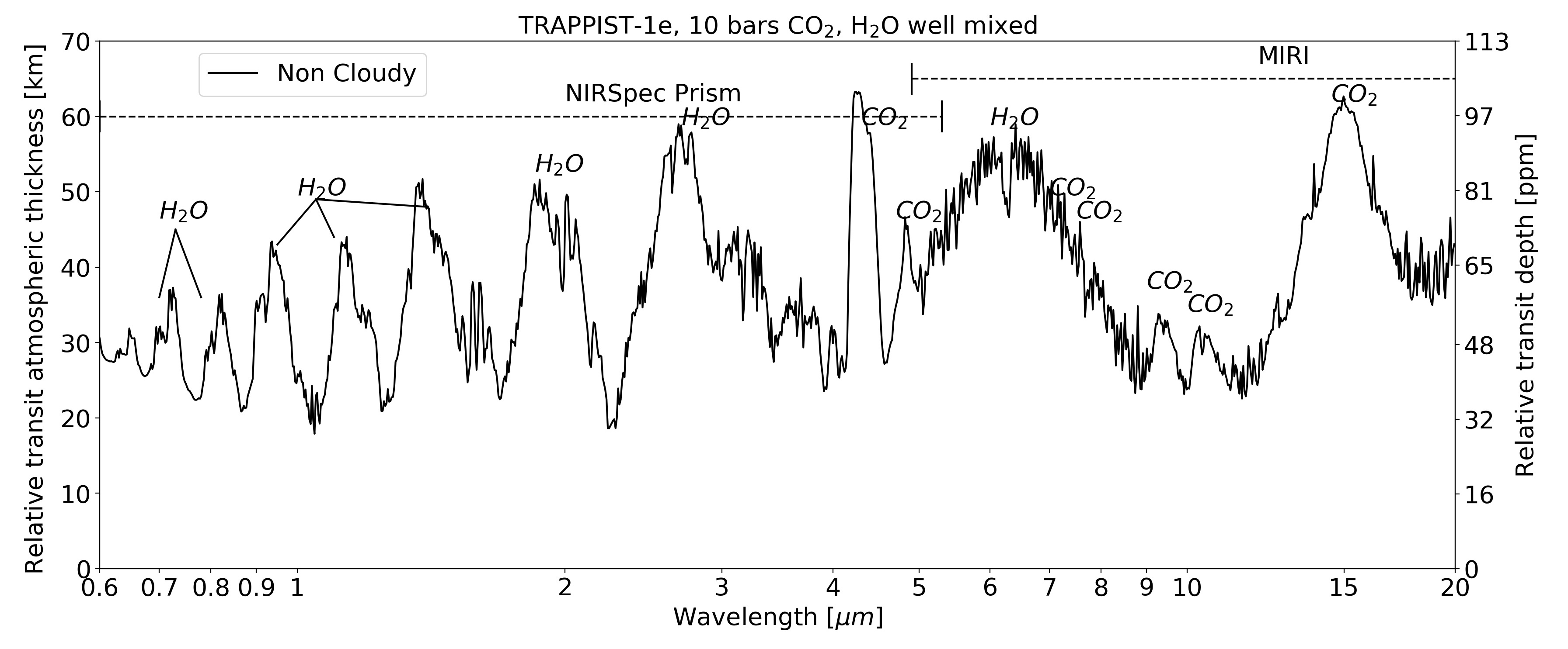
Figure 18: TRAPPIST-1e transmission spectrum for the 10 bars of CO₂ atmosphere for which H₂O has been forced to be vertically well-mixed. In transmission spectroscopy, H₂O are much stronger when H₂O is vertically well-mixed than when H₂O is confined near the surface.

Water vapor in the atmosphere intrinsically leads to water cloud formation either in the liquid or ice phase. Clouds are formed where the majority of the water vapor is in a non-runaway atmosphere, and they partially block the transmitted light, flattening the spectrum especially for H₂O. Well mixed species such as CO₂ are less impacted because enough of it remains above the cloud deck.

Concerning emission spectroscopy, this technique is more sensitive to hot planets near the star (Morley et al., 2017). The hottest simulations we have performed are TRAPPIST-1e at 10 bars of CO₂. Figure 19 shows the emission spectrum for MIRI from 5 to $20\ \mu m$ with a R=300 for the secondary eclipse. Below $5\ \mu m$, the contribution of the star removes the signal. The black curve shows the clear-sky spectrum and the blue curve shows the cloudy-sky spectrum. While few strong H₂O lines are present here in the clear-sky case, once clouds are considered those lines are flattened. The H₂O lines that are less impacted are near $20\ \mu m$, with a thermal contrast of 25 ppm, but this is much smaller than the noise in the MIRI and therefore will be hard to detect. Beyond $20\ \mu m$ clouds become more transparent and the planet/star contrast increases and the noise increases dramatically as well. Therefore, it seems that emission spectroscopy with JWST is not helpful to detect H₂O lines, in agreement with Lustig-Yaeger et al. (2019).

Reflection spectroscopy may be a better option to probe water vapor lines because, contrary to the transmission spectroscopy for which the starlight is transmitted through the terminator of the planet, it could probe the disk of the planet where clouds could be absent in some regions, at various phases. Also reflection spectroscopy can probe the lowest level of the atmosphere where most of the water resides. However, the small inner working angle (IWA) of the instrument on future direct imaging missions such as LUVOIR or HabEX would prevent the observation of such compact system like TRAPPIST-1.

The combination of the two effects: 1) the water vapor confined in the low atmosphere and 2) the cloud opacities imply that the detection of water vapor lines may be challenging to detect for planets in the habitable zone of TRAPPIST-1 or equivalent system.

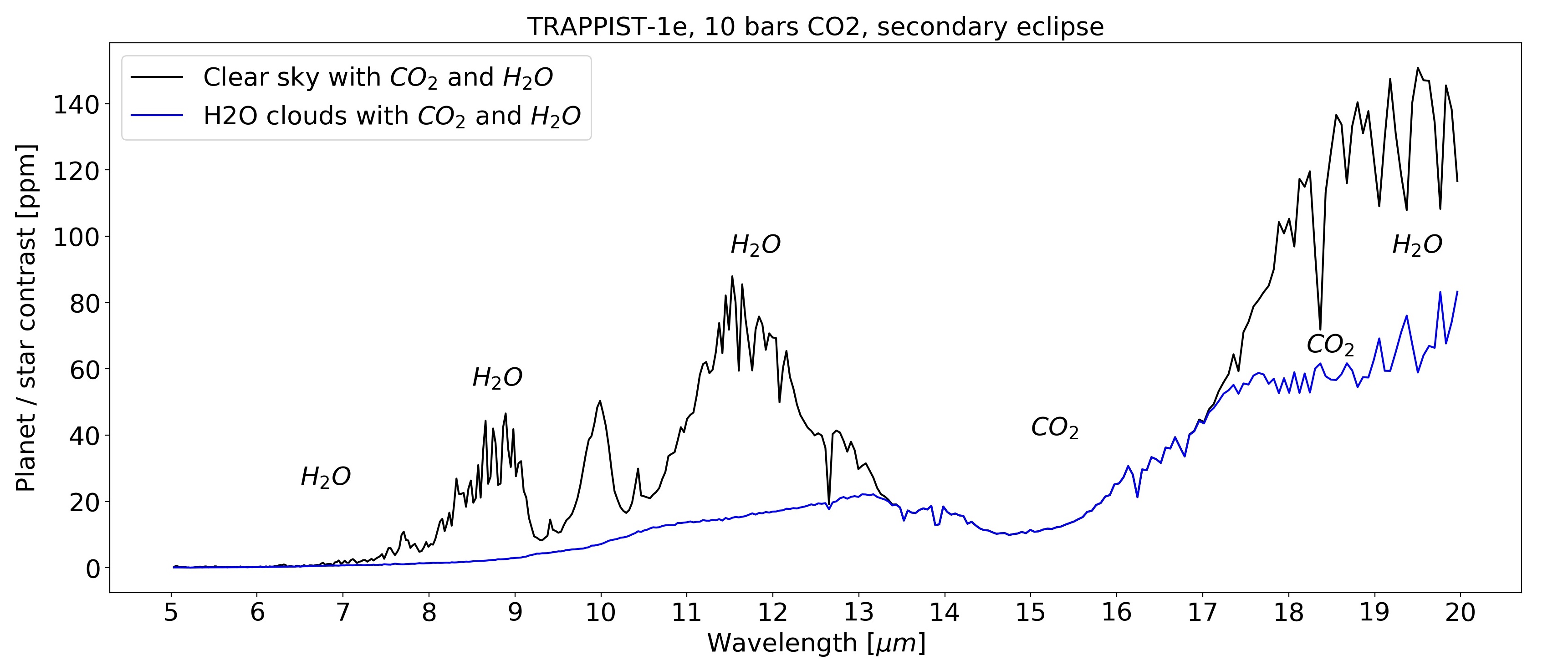
Figure 19: Emission spectrum from the secondary eclipse with MIRI (R=300) for TRAPPIST-1e with an atmosphere consisting of a surface pressure of 10 bars of CO₂.

7 Conclusions

In this work we have successfully connected a global circulation model (LMD-G) to a 1-D photochemical model (Atmos) and then applied a spectrum generator and noise model to estimate the detectability of gas species in a realistic set of possible atmospheres for the TRAPPIST-1 planets in the HZ. This has led to a consistent estimation of the cloud coverage along with the atmospheric temperatures and water profiles of tidally-locked planets around M dwarfs. However, the haze formation and photochemistry have been limited to the terminator region only, while a more consistent way would be to fully couple the GCM and the photochemical model. Also, no ocean heat transport has been considered (LMD-G does not have this feature yet) but that should not qualitatively impact our results. toward the terminator with OHT enabled. These effects will be investigated in future studies.

We have seen that the Archean Earth-like atmospheres offer habitable conditions (ice-free surface) for TRAPPIST-1e and TRAPPIST-1f while only TRAPPIST-1e is habitable if an atmosphere with boundary conditions based on the modern Earth is considered. The CO₂ atmospheres lead to very high surface temperatures. TRAPPIST-1e is fully habitable at 1 bar of CO₂ while TRAPPIST-1f is an eye-ball planet (TRAPPIST-1g atmosphere collapses at 1 bar of CO₂). At 10 bars of CO₂, TRAPPIST-1e and 1f surface temperatures are so high that the oceans should evaporate leading to desiccated planets. On the other hand, TRAPPIST-1g holds a few habitable ice-free spots near the substellar point.

Using the simulated JWST transmission spectroscopy, we found that an atmosphere with varying concentrations of CO₂ would be detectable for all habitable atmosphere configurations presented in this work in less than 15 transits at $3\ \sigma$ or less than 35 transits at $5\ \sigma$ with NIRSpec. Nevertheless, CO₂ is expected to be an abundant gas in an exoplanet atmosphere owing to its large abundance in the rocky planet atmospheres of our Solar system and to its high molecular weight making it more resistant to atmospheric escape. This number of transit observations is reasonably achievable during the lifetime of JWST. Unfortunately, we did not find any gas other than CO₂ to be detectable during JWST nominal life time or in less than 100 transits. Overall, it appears that NIRSpec performed better in terms of signal-to-noise ratio and minimizes the number of transits in comparison to MIRI. However, if hazes are detected on these planets, MIRI (in its shortest wavelengths between 5 to 10 $\mu m$) may perform better because the haze opacity is much lower than within the NIRSpec range. This study also suggests that it is very challenging to detect water lines for habitable planets orbiting ultra-cool dwarf stars such as TRAPPIST-1. Indeed, water mostly remains confined to the lower levels of the atmosphere with higher IR opacity leading to shallow lines (well below the noise floor of next space observatories), very often blended by stronger lines of the well-mixed CO₂. Water may be mixed through the entire atmospheric column if the planets are in a moist greenhouse state, but it will require either a very high amount of GHG (greater than 10 bars) and/or an instellation larger than the one received in the habitable zone and/or a very thin atmosphere suppressing cold traps. In addition, water vapor in the atmosphere implies the formation of water clouds blocking the transmitted light and leading to the flattening of water lines.

References

- Anderson et al. (2011) Anderson, D. R., Smith, A. M. S., Lanotte, A. A., et al. 2011, Monthly Notices of the Royal Astronomical Society, 416, 2108. https://doi.org/10.1111/j.1365-2966.2011.19182.x
- Anglada-Escudé et al. (2016) Anglada-Escudé, G., Amado, P. J., Barnes, J., et al. 2016, Nature, 536, 437
- Arney et al. (2016) Arney, G., Domagal-Goldman, S. D., Meadows, V. S., et al. 2016, Astrobiology, 16, 873
- Arney et al. (2017) Arney, G. N., Meadows, V. S., Domagal-Goldman, S. D., et al. 2017, ApJ, 836, 49
- Barnes (2017) Barnes, R. 2017, Celestial Mechanics and Dynamical Astronomy, 129, 509
- Barstow & Irwin (2016) Barstow, J. K., & Irwin, P. G. J. 2016, Monthly Notices of the Royal Astronomical Society, 461, L92
- Batalha et al. (2018) Batalha, N. E., Lewis, N. K., Line, M. R., Valenti, J., & Stevenson, K. 2018, The Astrophysical Journal, 856, L34. https://doi.org/10.3847%2F2041-8213%2Faab896
- Berta-Thompson et al. (2015) Berta-Thompson, Z. K., Irwin, J., Charbonneau, D., et al. 2015, Nature, 527, 204
- Bolmont et al. (2017) Bolmont, E., Selsis, F., Owen, J. E., et al. 2017, Monthly Notices of the Royal Astronomical Society, 464, 3728
- Bonfils et al. (2018) Bonfils, X., Astudillo-Defru, N., Díaz, R., et al. 2018, Astronomy and Astrophysics, 613, A25
- Boucher et al. (1995) Boucher, O., Le Treut, H., & Baker, M. B. 1995, Journal of Geophysical Research: Atmospheres, 100, 16395. https://agupubs.onlinelibrary.wiley.com/doi/abs/10.1029/95JD01382
- Bourrier et al. (2017) Bourrier, V., de Wit, J., Bolmont, E., et al. 2017, The Astronomical Journal, 154, 121. http://stacks.iop.org/1538-3881/154/i=3/a=121
- Burkholder et al. (2015) Burkholder, S. P. S., Abbatt, J., Barker, et al. 2015, Chemical Kinetics and Photochemical Data for Use in Atmospheric Studies, Tech. rep., Jet Propulsion Laboratory, Pasadena. http://jpldataeval.jpl.nasa.gov
- Carone et al. (2014) Carone, L., Keppens, R., & Decin, L. 2014, MNRAS, 445, 930
- Carone et al. (2015) —. 2015, MNRAS, 453, 2412
- Carone et al. (2018) Carone, L., Keppens, R., Decin, L., & Henning, T. 2018, MNRAS, 473, 4672
- Charnay et al. (2013) Charnay, B., Forget, F., Wordsworth, R., et al. 2013, Journal of Geophysical Research (Atmospheres), 118, 10,414
- Charnay et al. (2015a) Charnay, B., Meadows, V., & Leconte, J. 2015a, The Astrophysical Journal, 813, 15. https://doi.org/10.1088%2F0004-637x%2F813%2F1%2F15
- Charnay et al. (2015b) Charnay, B., Meadows, V., Misra, A., Leconte, J., & Arney, G. 2015b, The Astrophysical Journal, 813, L1. https://doi.org/10.1088%2F2041-8205%2F813%2F1%2Fl1
- Chen et al. (2018) Chen, H., Wolf, E. T., Kopparapu, R., Domagal-Goldman, S., & Horton, D. E. 2018, The Astrophysical Journal, 868, L6
- de Wit & Seager (2013) de Wit, J., & Seager, S. 2013, Science, 342, 1473
- de Wit et al. (2016) de Wit, J., Wakeford, H. R., Gillon, M., et al. 2016, Nature, 537, 69 EP . https://doi.org/10.1038/nature18641
- de Wit et al. (2018) de Wit, J., Wakeford, H. R., Lewis, N. K., et al. 2018, Nature Astronomy, 2, 214. https://doi.org/10.1038/s41550-017-0374-z
- Del Genio et al. (2019) Del Genio, A. D., Way, M. J., Amundsen, D. S., et al. 2019, Astrobiology, 19, 99, pMID: 30183335. https://doi.org/10.1089/ast.2017.1760
- Deming et al. (2009) Deming, D., Seager, S., Winn, J., et al. 2009, Publications of the Astronomical Society of the Pacific, 121, 952
- Dong et al. (2018) Dong, C., Jin, M., Lingam, M., et al. 2018, Proceedings of the National Academy of Science, 115, 260
- Forget & Pierrehumbert (1997) Forget, F., & Pierrehumbert, R. T. 1997, Science, 278, 1273
- Forget et al. (2013) Forget, F., Wordsworth, R., Millour, E., et al. 2013, Icarus, 222, 81
- Forget et al. (1999) Forget, F., Hourdin, F., Fournier, R., et al. 1999, Journal of Geophysical Research: Planets, 104, 24155. https://agupubs.onlinelibrary.wiley.com/doi/abs/10.1029/1999JE001025
- Gavilan et al. (2017) Gavilan, L., Broch, L., Carrasco, N., Fleury, B., & Vettier, L. 2017, The Astrophysical Journal Letters, 848, L5. http://stacks.iop.org/2041-8205/848/i=1/a=L5
- Gillon et al. (2016) Gillon, M., Jehin, E., Lederer, S. M., et al. 2016, Nature, 533, 221 . https://doi.org/10.1038/nature17448
- Gillon et al. (2017) Gillon, M., Triaud, A. H. M. J., Demory, B.-O., et al. 2017, Nature, 542, 456–460. https://doi.org/10.1038/nature21360
- Gillon et al. (2017b) Gillon, M., Demory, B.-O., Van Grootel, V., et al. 2017b, Nature Astronomy, 1, 0056
- Greene et al. (2016) Greene, T. P., Line, M. R., Montero, C., et al. 2016, The Astrophysical Journal, 817, 17
- Grenfell et al. (2014) Grenfell, J., Gebauer, S., v. Paris, P., Godolt, M., & Rauer, H. 2014, Planetary and Space Science, 98, 66 , planetary evolution and life. http://www.sciencedirect.com/science/article/pii/S0032063313002687
- Grimm et al. (2018) Grimm, S. L., Demory, B.-O., Gillon, M., et al. 2018, Astronomy and Astrophysics, 613, A68
- Haberle et al. (2017) Haberle, R. M., Zahnle, K., & Barlow, N. 2017, in LPI Contributions, Vol. 2014, Fourth International Conference on Early Mars: Geologic, Hydrologic, and Climatic Evolution and the Implications for Life, 3022
- Hansen et al. (1991) Hansen, G. B., Warren, S. G., & Leovy, C. B. 1991, Optical properties of CO2 ice and CO2 snow from ultraviolet to infrared: Application to frost deposits and clouds on Mars, Tech. rep.
- Hansen & Travis (1974) Hansen, J. E., & Travis, L. D. 1974, Space Science Reviews, 16, 527
- Harman et al. (2018) Harman, C. E., Felton, R., Hu, R., et al. 2018, The Astrophysical Journal, 866, 56. https://doi.org/10.3847%2F1538-4357%2Faadd9b
- Hourdin et al. (2006) Hourdin, F., Musat, I., Bony, S., et al. 2006, Climate Dynamics, 27, 787
- Hu & Yang (2014) Hu, Y., & Yang, J. 2014, Proceedings of the National Academy of Sciences, 111, 629. https://www.pnas.org/content/111/2/629
- Joshi (2003) Joshi, M. 2003, Astrobiology, 3, 415, pMID: 14577888. https://doi.org/10.1089/153110703769016488
- Joshi & Haberle (2012) Joshi, M. M., & Haberle, R. M. 2012, Astrobiology, 12, 3, pMID: 22181553. https://doi.org/10.1089/ast.2011.0668
- Kaltenegger & Traub (2009) Kaltenegger, L., & Traub, W. A. 2009, The Astrophysical Journal, 698, 519
- Kasting et al. (1993) Kasting, J. F., Whitmire, D. P., & Reynolds, R. T. 1993, Icarus, 101, 108 . http://www.sciencedirect.com/science/article/pii/S0019103583710109
- Khare et al. (1984) Khare, B. N., Sagan, C., Arakawa, E. T., et al. 1984, Icarus, 60, 127
- Kite (2019) Kite, E. S. 2019, Space Science Reviews, 215, 10
- Kitzmann (2017) Kitzmann, D. 2017, Astronomy Astrophysics, 600, A111
- Knutson et al. (2008) Knutson, H. A., Charbonneau, D., Allen, L. E., Burrows, A., & Megeath, S. T. 2008, ApJ, 673, 526
- Knutson et al. (2009) Knutson, H. A., Charbonneau, D., Cowan, N. B., et al. 2009, The Astrophysical Journal, 703, 769
- Kopparapu et al. (2017) Kopparapu, R. K., Wolf, E. T., Arney, G., et al. 2017, The Astrophysical Journal, 845, 5. http://stacks.iop.org/0004-637X/845/i=1/a=5
- Kopparapu et al. (2013) Kopparapu, R. K., Ramirez, R., Kasting, J. F., et al. 2013, The Astrophysical Journal, 765, 131. http://stacks.iop.org/0004-637X/765/i=2/a=131
- Kreidberg et al. (2014) Kreidberg, L., Bean, J. L., Désert, J.-M., et al. 2014, Nature, 505, 69
- Lacis & Oinas (1991) Lacis, A. A., & Oinas, V. 1991, Journal of Geophysical Research: Atmospheres, 96, 9027. https://agupubs.onlinelibrary.wiley.com/doi/abs/10.1029/90JD01945
- Lammer et al. (2009) Lammer, H., Bredehöft, J. H., Coustenis, A., et al. 2009, A&A Rev., 17, 181
- Leconte et al. (2013a) Leconte, J., Forget, F., Charnay, B., Wordsworth, R., & Pottier, A. 2013a, Nature, 504, 268
- Leconte et al. (2013b) Leconte, J., Forget, F., Charnay, B., et al. 2013b, Astronomy Astrophysics, 554, A69
- Leconte et al. (2015) Leconte, J., Wu, H., Menou, K., & Murray, N. 2015, Science, 347, 632. http://science.sciencemag.org/content/347/6222/632
- Lincowski et al. (2018) Lincowski, A. P., Meadows, V. S., Crisp, D., et al. 2018, The Astrophysical Journal, 867, 76
- Line & Parmentier (2016) Line, M. R., & Parmentier, V. 2016, The Astrophysical Journal, 820, 78
- Luger et al. (2017) Luger, R., Sestovic, M., Kruse, E., et al. 2017, Nature Astronomy, 1, 0129
- Lustig-Yaeger et al. (2019) Lustig-Yaeger, J., Meadows, V. S., & Lincowski, A. P. 2019, The Astronomical Journal, 158, 27. https://doi.org/10.3847%2F1538-3881%2Fab21e0
- Massie & Hervig (2013) Massie, S. T., & Hervig, M. 2013, J. Quant. Spec. Radiat. Transf., 130, 373
- Meadows & Crisp (1996) Meadows, V. S., & Crisp, D. 1996, J. Geophys. Res., 101, 4595
- Meadows et al. (2018) Meadows, V. S., Arney, G. N., Schwieterman, E. W., et al. 2018, Astrobiology, 18, 133, pMID: 29431479. https://doi.org/10.1089/ast.2016.1589
- Merlis & Schneider (2010) Merlis, T. M., & Schneider, T. 2010, Journal of Advances in Modeling Earth Systems, 2, 13
- Moran et al. (2018) Moran, S. E., Hörst, S. M., Batalha, N. E., Lewis, N. K., & Wakeford, H. R. 2018, The Astronomical Journal, 156, 252. http://stacks.iop.org/1538-3881/156/i=6/a=252
- Morley et al. (2017) Morley, C. V., Kreidberg, L., Rustamkulov, Z., Robinson, T., & Fortney, J. J. 2017, The Astrophysical Journal, 850, 121
- Nikolov et al. (2015) Nikolov, N., Sing, D. K., Burrows, A. S., et al. 2015, Monthly Notices of the Royal Astronomical Society, 447, 463
- O’Malley-James & Kaltenegger (2017) O’Malley-James, J. T., & Kaltenegger, L. 2017, Monthly Notices of the Royal Astronomical Society: Letters, 469, L26. http://dx.doi.org/10.1093/mnrasl/slx047
- Perrin & Hartmann (1989) Perrin, M. Y., & Hartmann, J. M. 1989, J. Quant. Spec. Radiat. Transf., 42, 311
- Pierrehumbert (1995) Pierrehumbert, R. T. 1995, Journal of Atmospheric Sciences, 52, 1784
- Quintana et al. (2014) Quintana, E. V., Barclay, T., Raymond, S. N., et al. 2014, Science, 344, 277
- Rajpurohit et al. (2013) Rajpurohit, A. S., Reylé, C., Allard, F., et al. 2013, Astronomy Astrophysics, 556, A15
- Richard et al. (2012) Richard, C., Gordon, I., Rothman, L., et al. 2012, Journal of Quantitative Spectroscopy and Radiative Transfer, 113, 1276 , three Leaders in Spectroscopy. http://www.sciencedirect.com/science/article/pii/S0022407311003773
- Rossow (1978) Rossow, W. B. 1978, Icarus, 36, 1
- Rothman et al. (2009) Rothman, L., Gordon, I., Barbe, A., et al. 2009, Journal of Quantitative Spectroscopy and Radiative Transfer, 110, 533 , hITRAN. http://www.sciencedirect.com/science/article/pii/S0022407309000727
- Rothman et al. (2010) Rothman, L., Gordon, I., Barber, R., et al. 2010, Journal of Quantitative Spectroscopy and Radiative Transfer, 111, 2139 , xVIth Symposium on High Resolution Molecular Spectroscopy (HighRus-2009). http://www.sciencedirect.com/science/article/pii/S002240731000169X
- Segura et al. (2003) Segura, A., Krelove, K., Kasting, J. F., et al. 2003, Astrobiology, 3, 689, pMID: 14987475. https://doi.org/10.1089/153110703322736024
- Selsis et al. (2007) Selsis, F., Kasting, J. F., Levrard, B., et al. 2007, A&A, 476, 1373
- Shields et al. (2013) Shields, A. L., Meadows, V. S., Bitz, C. M., et al. 2013, Astrobiology, 13, 715
- Showman & Polvani (2011) Showman, A. P., & Polvani, L. M. 2011, ApJ, 738, 71
- Sing et al. (2016) Sing, D. K., Fortney, J. J., Nikolov, N., et al. 2016, Nature, 529, 59
- Snellen et al. (2013) Snellen, I. A. G., de Kok, R. J., le Poole, R., Brogi, M., & Birkby, J. 2013, The Astrophysical Journal, 764, 182
- Toon et al. (1989) Toon, O. B., McKay, C. P., Ackerman, T. P., & Santhanam, K. 1989, Journal of Geophysical Research: Atmospheres, 94, 16287. https://agupubs.onlinelibrary.wiley.com/doi/abs/10.1029/JD094iD13p16287
- Tsiaras et al. (2016) Tsiaras, A., Rocchetto, M., Waldmann, I. P., et al. 2016, The Astrophysical Journal, 820, 99. https://doi.org/10.3847%2F0004-637x%2F820%2F2%2F99
- Turbet et al. (2017a) Turbet, M., Forget, F., Head, J. W., & Wordsworth, R. 2017a, Icarus, 288, 10
- Turbet et al. (2017b) Turbet, M., Forget, F., Leconte, J., Charnay, B., & Tobie, G. 2017b, Earth and Planetary Science Letters, 476, 11
- Turbet et al. (2016) Turbet, M., Leconte, J., Selsis, F., et al. 2016, Astronomy and Astrophysics, 596, A112
- Turbet et al. (2018) Turbet, M., Bolmont, E., Leconte, J., et al. 2018, Astronomy and Astrophysics, 612, A86
- Vida & Roettenbacher (2018) Vida, K., & Roettenbacher, R. M. 2018, Astronomy and Astrophysics, 616, A163
- Villanueva et al. (2018) Villanueva, G. L., Smith, M. D., Protopapa, S., Faggi, S., & Mandell, A. M. 2018, Journal of Quantitative Spectroscopy and Radiative Transfer, 217, 86
- von Paris et al. (2013) von Paris, P., Selsis, F., Kitzmann, D., & Rauer, H. 2013, Astrobiology, 13, 899
- Wakeford et al. (2017) Wakeford, H. R., Visscher, C., Lewis, N. K., et al. 2017, MNRAS, 464, 4247
- Warren (1984) Warren, S. G. 1984, Annals of Glaciology, 5, 177
- Warren & Wiscombe (1980) Warren, S. G., & Wiscombe, W. J. 1980, Journal of the Atmospheric Sciences, 37, 2734. https://doi.org/10.1175/1520-0469(1980)037<2734:AMFTSA>2.0.CO;2
- Way et al. (2017) Way, M. J., Aleinov, I., Amundsen, D. S., et al. 2017, The Astrophysical Journal Supplement Series, 231, 12. http://stacks.iop.org/0067-0049/231/i=1/a=12
- Wheatley et al. (2017) Wheatley, P. J., Louden, T., Bourrier, V., Ehrenreich, D., & Gillon, M. 2017, Monthly Notices of the Royal Astronomical Society: Letters, 465, L74. http://dx.doi.org/10.1093/mnrasl/slw192
- Winn (2010) Winn, J. N. 2010, arXiv e-prints, arXiv:1001.2010
- Wolf (2017) Wolf, E. T. 2017, The Astrophysical Journal Letters, 839, L1. http://stacks.iop.org/2041-8205/839/i=1/a=L1
- Wolf & Toon (2015) Wolf, E. T., & Toon, O. B. 2015, Journal of Geophysical Research: Atmospheres, 120, 5775. https://agupubs.onlinelibrary.wiley.com/doi/abs/10.1002/2015JD023302
- Wordsworth et al. (2010) Wordsworth, R., Forget, F., & Eymet, V. 2010, Icarus, 210, 992 . http://www.sciencedirect.com/science/article/pii/S0019103510002320
- Wordsworth et al. (2013) Wordsworth, R., Forget, F., Millour, E., et al. 2013, Icarus, 222, 1 . http://www.sciencedirect.com/science/article/pii/S0019103512004290
- Wordsworth et al. (2011) Wordsworth, R. D., Forget, F., Selsis, F., et al. 2011, The Astrophysical Journal Letters, 733, L48. http://stacks.iop.org/2041-8205/733/i=2/a=L48
- Wordsworth et al. (2015) Wordsworth, R. D., Kerber, L., Pierrehumbert, R. T., Forget, F., & Head, J. W. 2015, Journal of Geophysical Research (Planets), 120, 1201
- Yang et al. (2014) Yang, J., Boué, G., Fabrycky, D. C., & Abbot, D. S. 2014, The Astrophysical Journal, 787, L2
- Yang et al. (2013) Yang, J., Cowan, N. B., & Abbot, D. S. 2013, The Astrophysical Journal, 771, L45. https://doi.org/10.1088%2F2041-8205%2F771%2F2%2Fl45
- Zahnle et al. (2010) Zahnle, K., Schaefer, L., & B., F. 2010, Cold Spring Harb Perspect Biol., 2, 17p
- Zmuidzinas (2003) Zmuidzinas, J. 2003, Appl. Opt., 42, 4989. http://ao.osa.org/abstract.cfm?URI=ao-42-25-4989