Alternating knots with large boundary slope diameter

Abstract.

We show that, for an alternating knot, the ratio of the diameter of the set of boundary slopes to the crossing number can be arbitrarily large.

1. Introduction

Let $K$ be a knot in $S^{3}$ and $c(K)$ the crossing number of $K$. The diameter of the set of boundary slopes of $K$, denoted by $\text{\rm diam}(K)$, is the difference, as rational numbers, between the maximal boundary slope and the minimal boundary slope of $K$. We show that, for alternating knots, the ratio of the diameter of the boundary slopes to the crossing number can be arbitrarily large.

Curtis and Taylor  [2] showed the diameter of the boundary slopes of essential spanning surfaces of an alternating knot $K$ is $2c(K)$. See also [6]. Ichihara and Mizushima [7] argued that, for a Montesinos knot $K$, the ratio $\frac{\text{\rm diam}(K)}{c(K)}$ is at most two, with equality if and only if $K$ is alternating. In fact, they showed $\frac{\text{\rm diam}(K)}{c(K)}\geq 2$ in the case of alternating knots (whether or not they are Montesinos). According to Culler’s calculation of the A-polynomial [1], the $8$–crossing non-Montesinos alternating knots $8_{17}$ and $8_{18}$ have boundary slopes $-14$ and $14$ so that the diameter is at least $28$, which is larger than twice the crossing number. Those calculations are confirmed by Kabaya, who, by applying his method for the deformation variety [9], also demonstrated diameters in excess of twice the crossing number for the alternating knots $9_{32}$, $9_{33}$, $9_{34}$, $9_{39}$, $10_{82}$, and $10_{94}$. In the case of $9_{39}$, he showed the diameter is at least $30$, which is more than three times the crossing number [8]. Dunfield and Garoufalidis [3] also constructed interesting examples of alternating knots with rational boundary slopes using spun-normal surfaces.

Here we prove that, for an alternating knot, the ratio of the diameter of the boundary slopes to the crossing number can be arbitrarily large.

Theorem 1.1.

For any positive number $r$, there exists an alternating knot $K$ such that the ratio $\frac{\text{\rm diam}(K)}{c(K)}>r$. In particular, there is a sequence of alternating knots $\{K_{n}\}_{n=1}^{\infty}$ such that ${\displaystyle\lim_{c(K_{n})\to\infty}}\frac{\text{\rm diam}(K_{n})}{c(K_{n})}=\infty$.

We adapt Hatcher and Oertel’s [5] method for Montesinos knots to arborescent knots formed as the product of two Montesinos tangles. In the next section we give a framework for such knots and in Section 3 we describe how to construct candidate surfaces from edgepaths in this setting. Section 4 shows how to calculate the corresponding boundary slopes. Finally, in Section 5 we prove our main theorem.

2. Arborescent knots

In this article, a tangle $(B,T)$ is a pair of a 3-ball $B$ and its properly embedded 1-submanifold $T$ in $B$ with 4 boundary points NE, NW, SE and SW. Sometimes a tangle is simply denoted by $T$. We assume that $B$ is embedded in $\mathbb{R}^{3}$ and the four points NE, NW, SE and SW are on a plane $P$ in $\mathbb{R}^{3}$. A rational tangle is a tangle that is homeomorphic to the pair $(D\times[0,1],\{p_{1},p_{2}\}\times[0,1])$, where $D$ is a disk and $p_{1}$ and $p_{2}$ are points in the interior of $D$.

Definition 2.1.

Let $(B_{1},T_{1})$ and $(B_{2},T_{2})$ be two tangles. We identify the right hemisphere of $\partial B_{1}$ and the left hemisphere of $\partial B_{2}$ to form a tangle $(B_{1}\cup B_{2},T_{1}\cup T_{2})$. The resulting tangle is denoted by $T_{1}+T_{2}$ and called the tangle sum of $T_{1}$ and $T_{2}$. For rational tangles $(B_{1},R_{1}),\cdots,(B_{n},R_{n})$, the tangle sum $R_{1}+\cdots+R_{n}$ is called a Montesinos tangle. Let $\Delta_{i}$ be the disk $B_{i}\cap B_{i+1}$. Let $A$ be $\partial\Delta_{i}$. The loop $A$ is called the axis of the Montesinos tangle.

Definition 2.2.

Let $R$ and $T$ be tangles. Let $R^{\prime}$ denote the tangle that results from $\frac{\pi}{2}$-rotation of the reflection of $R$. Here the reflection means the tangle obtained by exchanging “over” and “under” at all crossings in the tangle. Then the tangle product of $R$ and $T$, denoted $R\circ T$ is the sum $R^{\prime}+T$. See Figure 1. We also define the axis of $R\circ T$ as the union of the boundaries of the left and right hemispheres of the attaching tangles.

Figure 1. Tangle sum and product. $R^{*}$ denotes the reflection of $R$. $R^{\prime}$ is the tangle that results from $\frac{\pi}{2}$-rotation of $R^{*}$ .

Definition 2.3.

Let $(B,T)$ be a tangle. We can construct a knot or a link by connecting NE and NW with an arc in $P\cap\partial B$ and SE and SW with an arc in $P\cap\partial B$. This knot or link is denoted by $N(T)$ and called the numerator of $T$.

Definition 2.4.

A knot $K$ is an SN knot if there are Montesinos tangles $T_{1}$ and $T_{2}$ such that $K=N(T_{1}\circ T_{2})$. We call $T_{2}$ the outer tangle. The tangle obtained from $T_{1}$ by $\frac{\pi}{2}$-rotation of the reflection will be denoted $T_{1}^{\prime}$ and called the inner tangle.

Note that for an alternating Montesinos tangle $T$, the SN knot $N(T\circ T)$ is also alternating.

Definition 2.5.

A tangle is called an algebraic tangle if it is obtained by a finite sequence of tangle sums and tangle products of rational tangles. The numerator $N(T)$ of an algebraic tangle $T$ is called an arborescent knot or link.

Note that the numerator of $(B,T)$ can be obtained by identifying the left hemisphere of $B$ with the right one. If an algebraic tangle $T$ is made of rational tangles $(B_{1},R_{1}),\cdots,(B_{n},R_{n})$, then the arborescent knot $N(T)$ is in the $S^{3}$ that is the union of the $3$-balls $B_{1}\cup\cdots\cup B_{n}$. The union of all the axes is an embedded graph in $S^{3}$.

3. Candidate surfaces and edgepaths

In this section we describe how to build candidate surfaces from edgepaths in the context of an arborescent knot. We closely follow the discussion of Hatcher and Oertel [5] and begin with a review of some terminology from that paper. In Figure 2, we show the train track with weight $(a,b,c)$. The triple $(a,b,c)$ also labels a point of the Diagram $\mathcal{D}$ in [5] with vertical coordinate “slope” $v=\frac{c}{a+b}$ and horizontal coordinate $u=\frac{b}{a+b}$. Let $\langle\frac{p}{q}\rangle$ denote the point $(1,q-1,p)$.

Given such a train track, Hatcher and Oertel describe how to construct an edgepath $\gamma_{i}$ with the following four properties:

• The starting point of $\gamma_{i}$ lies on the edge $\langle\frac{p_{i}}{q_{i}},\frac{p_{i}}{q_{i}}\rangle$, and if the starting point is not the vertex $\langle\frac{p_{i}}{q_{i}}\rangle$, then the edgepath $\gamma_{i}$ is constant.

• $\gamma_{i}$ is minimal, i.e., it never stops and retraces itself, nor does it go along two sides of the same triangle of $\mathcal{D}$ in succession.

• The ending points of the $\gamma_{i}$’s are all rational points of $\mathcal{D}$ which all lie in one vertical line and whose vertical coordinates add up to zero.

• $\gamma_{i}$ proceeds monotonically from right to left, “monotonically” in a weak sense that motion along vertical edges is permitted.

As in [5], from an edgepath $\gamma_{i}$ we can construct a surface $S_{i}$ in $B_{i}$ with $\partial S_{i}\subset\partial B_{i}\cup K$, which we will call the surface $S_{i}$ given by the edgepath $\gamma_{i}$. So far, except for property E3, we have described Hatcher and Oertel’s construction for an individual rational tangle $(B_{i},R_{i})$.

Figure 2. A train track with weight $(a,b,c)$. The right figure has $t$ $\infty$-edges.

Now, let $K$ be an arborescent knot made from rational tangles $(B_{1},R_{1}),\cdots,(B_{n},R_{n})$. We will construct a properly embedded surface in the exterior of $K$ using the $S_{i}$’s given by the edgepaths $\gamma_{i}$. As an arborescent knot can be constructed by a sequence of tangle sums and tangle products, we take these operations in turn, starting with the sum.

Lemma 3.1 ([5]).

Let $T_{1}$ and $T_{2}$ be tangles with surfaces $\hat{S}_{1}$ and $\hat{S}_{2}$ having train tracks with weights $(a_{1},b_{1},c_{1})$ and $(a_{2},b_{2},c_{2})$ on the boundary, respectively. Suppose $a_{1}=a_{2}$ and $b_{1}=b_{2}$. Then we can construct a surface $S$ in $T_{1}+T_{2}$ for the triple $(a_{1},b_{1},c_{1}+c_{2})$ by gluing $\hat{S}_{1}$ and $\hat{S}_{2}$ canonically.

Next we consider the tangle product. The tangle product can be obtained by a sequence of operations consisting of $\frac{\pi}{2}$-rotation, reflection, and tangle sum. In the next lemma, we will consider how the weight of the train track is changed by $\frac{\pi}{2}$-rotation and reflection.

Lemma 3.2.

Let $T$ be a tangle with surface having a train track with weight $(a,b,c)$ on the boundary. Then the weight $(x,y,z)$ of the train track of the tangle $T^{\prime}$ obtained from $T$ by $\frac{\pi}{2}$-rotation and reflection satisfies the following in the case $c>0$ (respectively, $c<0$).

1. If $T$ has neither slope $0$ edges nor slope $\infty$ edges, then $(x,y,z)=(a,c-a,a+b)$ (resp. $(a,|c|-a,-(a+b))$).

2. If $T$ has slope 0 edges and does not have slope $\infty$ edges, then, $T^{\prime}$ has $a-|c|$ slope $\infty$ edges and triple $(x,y,z)=(c,0,b+c)$ (resp., $(|c|,0,-(b+|c|))$).

3. If $T$ does not have slope $0$ edges and has $t$ slope $\infty$ edges where $t<a$, then $(x,y,z)=(a,c-a+t,a-t)$ (resp. $(a,|c|-a+t,t-a)$).

4. If $T$ has both slope $0$ edges and $t$ slope $\infty$ edges, where $t<a-|c|$, then $T^{\prime}$ has $a-t-|c|$ slope $\infty$ edges and triple $(x,y,z)=(c+t,0,c)$ (resp. $(|c|+t,0,-c)$).

Proof.

We show the assertion in Case (1). In this case, the train track for $T$ is the one shown on the left in Figure 2. If $c>0$ then the $\frac{\pi}{2}$-rotation of its reflection becomes the train track on the top left in Figure 3. Then the assertion follows from the isotopy shown in Figure 3. If $c<0$, the isotopy is given by the mirror image of the isotopy in Figure 3.

The assertions for Cases (2), (3) and (4) follow from the isotopies shown in Figures 4, 5 and 6, respectively. ∎

Figure 3. Case (1) : $T$ has neither slope $0$ edges nor slope $\infty$ edges.

Figure 4. Case (2) : $T$ has slope $0$-edges. Then $T^{\prime}$ has $a-c$ slope $\infty$ edges.

Figure 5. Case (3) : $T$ has $t$ slope $\infty$ edges with $t<a$.

Figure 6. Case (4) : $T$ has $t$ slope $\infty$ edges with $t<a-c$. Then $T^{\prime}$ has $a-t-c$ slope $\infty$ edges.

To construct a candidate surface of an arborescent knot $K$, we replace property E3 of Hatcher and Oertel with the following.

• The ending points of the $\gamma_{i}$’s are all rational points of $\mathcal{D}$ chosen so that the surfaces $S_{i}$ given by the edgepaths $\gamma_{i}$ constitute a surface bounded by the knot $K$. We can easily check if the $S_{i}$ constitute a surface using Lemmas 3.1 and 3.2.

Note that, in [10], Wu studied exceptional surgeries of large arborescent knots. The class of SN knots in our paper includes knots of type II in [10]. In that paper, he used a different train track that works especially well for knots of type II. In our paper, we follow the notation of Hatcher and Oertel to emphasize that the observations in Lemmas 3.1 and 3.2 work for any arborescent knot. In fact, these lemmas work for any tangle with a train track.

4. Calculation of boundary slopes

In this section we will calculate the boundary slope of a candidate surface $S$ of an arborescent knot. Let $(B_{1},R_{1}),\cdots,(B_{n},R_{n})$ be rational tangles constituting an arborescent knot. For each surface $S_{i}$ in $B_{i}$ given by an edgepath, we define $\tau(S_{i})$ to be $\tau(S_{i})=2(e_{-}-e_{+})$, where $e_{+}$ (resp. $e_{-}$) is the number of edges of the edgepath which increase (resp. decrease) slope, allowing fractional values for $e_{\pm}$ corresponding to a final edge traversing only a fraction of an edge of the diagram $\mathcal{D}$. See [5, page 460] for a precise explanation. This number $\tau(S_{i})$ counts how many times the surface $S_{i}$ rotates around the knot in $B_{i}$. In particular, if $S_{i}$ is given by a constant edgepath then we have $\tau(S_{i})=0$. In [5], $\tau(S)$ is defined to be the sum of these numbers for rational tangles constituting a Montesinos knot. We use the same idea for arborescent knots.

Let $\hat{S}$ be a surface in an algebraic tangle $T$ obtained by gluing surfaces given by edgepaths in the rational tangles constituting $T$. We call $\hat{S}$ a surface given by edgepaths. We define $\tau(\hat{S})$ by applying Definitions 4.1 and 4.2 below inductively.

The first definition is for a tangle sum.

Definition 4.1.

Let $T_{1}$ and $T_{2}$ be algebraic tangles with surfaces $\hat{S}_{1}$ and $\hat{S}_{2}$, given by edgepaths, with the triples $(a,b,c_{1})$ and $(a,b,c_{2})$, respectively. Let $\hat{S}$ be the surface in $T_{1}+T_{2}$ with the triple $(a_{1},b_{1},c_{1}+c_{2})$ obtained by gluing $\hat{S}_{1}$ and $\hat{S}_{2}$, whose existence is stated in Lemma 3.1. Then $\tau(\hat{S})$ is defined by $\tau(\hat{S})=\tau(\hat{S}_{1})+\tau(\hat{S}_{2})$.

Before giving the second definition, we define $\tau^{\prime}(\hat{S})$, which measures how much the surface rotates along the knot during the isotopies in Figures 3 through 6. Let $T$ be a tangle with a candidate surface $\hat{S}$ having triple $(a,b,c)$ and $\hat{S}^{\prime}$ be the surface obtained from $\hat{S}$ by one of the isotopies shown in Figures 3 through 6. Set $m$ to be the number of sheets that rotate around the knot during the isotopy. Note that $m=a$ in Case (1), $m=c$ in Cases (2) and (4) and $m=a-t$ in Case (3), where $t$ is the number of slope $\infty$ edges in $T$. We define $\tau^{\prime}(\hat{S})$ as follows.

$$\tau^{\prime}(\hat{S})=\begin{cases}-\frac{2m}{a}\quad\text{if}\quad c>0\\ \frac{2m}{a}\quad\text{if}\quad c<0.\end{cases}$$

Definition 4.2.

Let $T_{1}$ and $T_{2}$ be algebraic tangles with surfaces $\hat{S}_{1}$ and $\hat{S}_{2}$ given by edgepaths, respectively. Suppose that $\hat{S}_{1}$ and $\hat{S}_{2}$ are glued in $T_{1}\circ T_{2}$ canonically as in Lemma 3.1 after the $\frac{\pi}{2}$-rotation and reflection of $T_{1}$ for the tangle product. Let $\hat{S}$ denote this surface in $T_{1}\circ T_{2}$. Then $\tau(\hat{S})$ is defined by $\tau(\hat{S})=-\tau(\hat{S}_{1})+\tau^{\prime}(\hat{S}_{1})+\tau(\hat{S}_{2})$.

The value $\tau$ for a candidate surface of an arborescent knot is then defined as follows.

Definition 4.3.

Suppose that an arborescent knot $K$ is the numerator of an algebraic tangle $T$, i.e., $N(T)=K$, and let $S$ be a candidate surface of $K$ obtained from a surface in $T$ given by edgepaths. Then $\tau(S)$ is defined by $\tau(S)=\tau(\hat{S})$.

To get the boundary slope of the candidate surface $S$ from $\tau(S)$, we need to determine $\tau(S_{0})$ for a Seifert surface $S_{0}$. Remark that we use the same tangle decomposition of $K$ when we calculate $\tau(S)$ and $\tau(S_{0})$.

Lemma 4.4.

Let $K$ be an arborescent knot consisting of Montesinos tangles including a rational tangle with even denominator and let $S_{0}$ be a Seifert surface of $K$. Then $\tau(S_{0})$ is the sum of $(-1)^{k_{i}}\tau(S_{i})$ for all Montesinos tangles $T_{i}$ constituting $K$, where $k_{i}$ is the number of reflections applied to the tangle $T_{i}$.

Proof.

As in [5], we find a piece of the Seifert surface for each Montesinos tangle $(B_{i},T_{i})$. In particular, the slopes of the surfaces in these tangles are $\infty$. When we make a tangle product, we take the reflection of $B_{i}$ and rotate it by $\frac{\pi}{2}$. Therefore, its slope becomes $0$ after the rotation. To glue this with other pieces, we add a saddle near $\partial B_{i}$ that changes the slope from $0$ to $\infty$. We can find suitable edgepaths whose surface can be glued with keeping the orientability when each Montesinos tangle contains a rational tangle with even denominator, see the explanation in [5, page 461]. The surface so constructed is single sheeted and orientable, hence a Seifert surface. Since adding a saddle does not change the number of twists around the knot, the contribution to $\tau(S_{0})$ of this adjustment is $0$. Hence the assertion follows. ∎

Lemma 4.5.

Let $S$ be a candidate surface of an arborescent knot. Then $\tau(S)-\tau(S_{0})$ is the boundary slope of $S$.

Proof.

As in [5], the value of $\tau$ can be determined by checking how the surface rotates around the knot. This rotation number is additive for a tangle sum. Hence the rotation number of the surface in $T_{1}+T_{2}$ obtained from surfaces $\hat{S}_{1}$ and $\hat{S}_{2}$ in $T_{1}$ and $T_{2}$, respectively, given by edgepaths, as mentioned in Lemma 3.1, is $\tau(\hat{S}_{1})+\tau(\hat{S}_{2})$. This is formulated in Definition 4.1. Next we observe the tangle product $T_{1}\circ T_{2}$ with surfaces $\hat{S}_{1}$ and $\hat{S}_{2}$ given by edgepaths. Remember that the tangle product can be obtained by a sequence of operations consisting of $\frac{\pi}{2}$-rotation, reflection of $T_{1}$, and tangle sum. Since $\hat{S}^{\prime}_{1}$ is the reflection of $\hat{S}_{1}$, the contribution of the twists of $\hat{S}_{1}$ to $\hat{S}^{\prime}_{1}$ is $-\tau(\hat{S}_{1})$. The contribution during the isotopy in Figures 3 through 6 is the value $\tau^{\prime}(\hat{S}_{1})$, which can be verified directly from those figures. Therefore, the rotation number becomes $-\tau(\hat{S}_{1})+\tau^{\prime}(\hat{S}_{1})+\tau(\hat{S}_{2})$ as in Definition 4.2. Thus $\tau(S)$ counts the rotation of $S$ around the knot correctly. The boundary slope of $S$ is given by the difference $\tau(S)-\tau(S_{0})$ as in [5]. ∎

5. Proof of Theorem 1.1

For $n\geq 2$, let $K_{n}$ denote the SN knot $N((-\frac{1}{n}+\frac{1}{n+1})\circ(-\frac{1}{n}+\frac{1}{n+1}))$, see Figure 7. Note that $K_{n}$ is achiral. Here $K_{n}=N(T_{1}\circ T_{2})$ and $(B_{1},T_{1})=(B_{1,1},T_{1,1})+(B_{1,2},T_{1,2})$ and $(B_{2},T_{2})=(B_{2,1},T_{2,1})+(B_{2,2},T_{2,2})$. Let $A_{i}$ be the axis defined by $\partial(B_{i,1}\cap B_{i,2})$ ($i=1,2$).

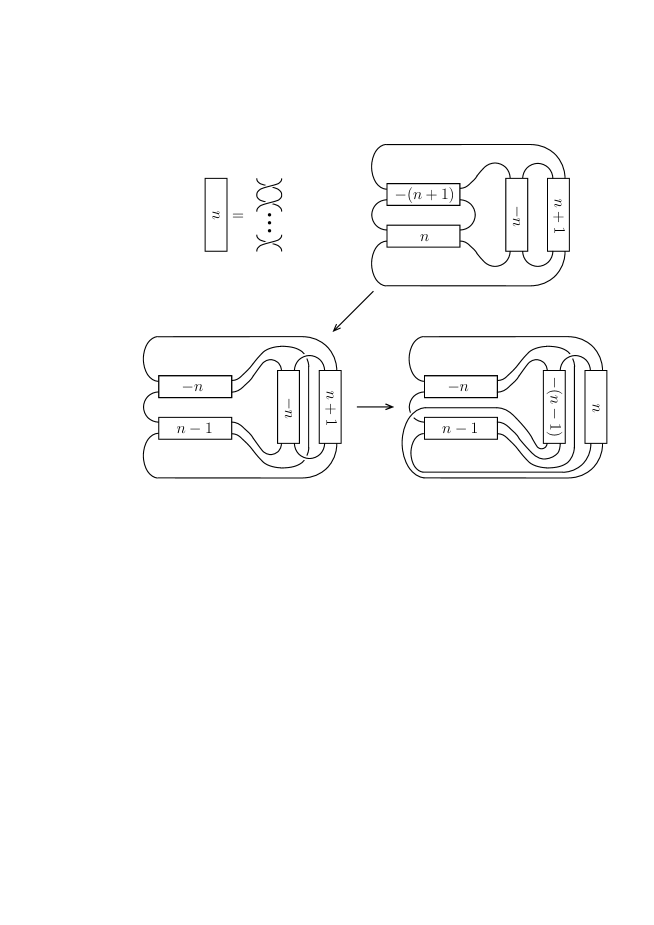
Figure 7. $K_{n}$ is an alternating knot with crossing number $4n$. The number $n$ in a box means the right-handed $n$ half twists and $-n$ in a box means the left-handed $n$ half twists.

Proposition 5.1.

$-2(n+1)^{2}+4$ and $2(n+1)^{2}-4$ are boundary slopes of essential spanning surfaces of $K_{n}$.

Proof.

Since $K_{n}$ is achiral, it is enough to show that $-2(n+1)^{2}+4$ is the boundary slope of an essential spanning surface. For this, we describe the surface in terms of edgepaths in $T_{1}=T_{2}=-\frac{1}{n}+\frac{1}{n+1}$. In $T_{1}$, we use constant edgepaths in both the $-\frac{1}{n}$ and $\frac{1}{n+1}$ rational tangles. Let the triples for the two rational tangles be $(1,n^{2}+n-1,-n-1)$ and $(1,n^{2}+n-1,n)$ so that $(1,n^{2}+n-1,-1)$ is the triple for $T_{1}$. As there are neither $0$-edges nor $\infty$-edges, by Lemma 3.2, the triple of $T_{1}$ after reflection, $\frac{\pi}{2}$-rotation and isotopy is $(1,0,-n^{2}-n)$. Therefore the triple of $T_{2}$ must be $(1,0,n^{2}+n)$. We choose the edgepaths of the $-\frac{1}{n}$ and $\frac{1}{n+1}$ tangles in $T_{2}$ as $\langle-\frac{1}{n}\rangle\to\langle 0\rangle$ and $\langle\frac{1}{n+1}\rangle\to\langle\frac{1}{n}\rangle\to\cdots\to\langle\frac{1}{2}\rangle\to\langle 1\rangle\to\cdots\to\langle n^{2}+n\rangle$, respectively.

Let $S$ be the candidate surface obtained from these edgepaths. We must argue that the candidate surface $S$ is incompressible. We adapt the arguments of Hatcher and Oertel [5] to this case. Let $D$ be a compressing disk of $S$ in $E(K)$. We may assume that $D$ meets $\partial B_{i}$ and $A_{i}$ transversely and misses the intersection points $A_{i}\cap A_{j}$. Set $G=D\cap(\partial B_{1}\cup\partial B_{2})$, which is a graph in $D$. We assume that the number of components of $G$ is minimal among all compressing disks for $S$.

If $G$ contains a loop that does not meet vertices, then by a surgery along an innermost disk of $D$, we will have another compressing disk whose graph has fewer components, a contradiction. Hence there is no loop without vertices in $G$.

We next argue that $D\cap B_{1}\neq\emptyset$. For a contradiction, assume $D\cap B_{1}$ is empty. Let $(B_{2,1},T_{2,1})$ and $(B_{2,2},T_{2,2})$ denote the $-\frac{1}{n}$ and $\frac{1}{n+1}$ tangles in $B_{2}$, respectively.

Suppose that edgemost disks are contained in $B_{2,1}$. Let $D^{\prime}$ be an edgemost disk that is bounded by the union of an arc $\alpha$ on $B_{2,1}\cap B_{2,2}$ and an arc $\beta$ on $\partial D$, see Figure 8 (left). Since the edgepath of $T_{2,1}$ is $\langle-\frac{1}{n}\rangle\to\langle 0\rangle$, the piece $S\cap B_{2,1}$ of the candidate surface $S$ in $B_{2,1}$ is a band as shown on the right in Figure 8. Then the disk $D^{\prime}$ either lies in the position shown in the figure or is bounded by $\alpha\cup\beta$ such that the endpoints of $\alpha$ lie on the same connected arc of $S\cap\partial B_{2,1}$. The latter case can be removed by isotopy of $D^{\prime}$. Consider the former case. The assumption $D\cap B_{1}=\emptyset$ implies that the arc $\alpha$ does not intersect the hemisphere $B_{1}\cap B_{2,1}$. Since the band $S\cap B_{2,1}$ is twisted $n$ times, there exists such a disk $D^{\prime}$ if and only if $|n|\leq 1$. In particular, if $n\geq 2$ then $D^{\prime}$ and $B_{1}$ should intersect. This contradicts the assumption that $D\cap B_{1}$ is an empty set.

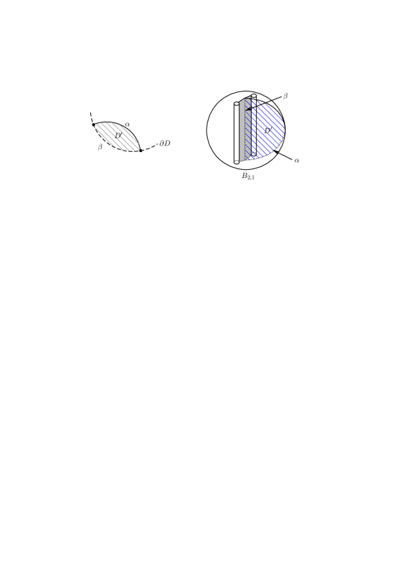
Figure 8. The edgemost disk $D^{\prime}$ in $B_{2,1}$.

Suppose that edgemost disks are in $B_{2,2}$. Then there is a disk $\Delta$ in $D$ contained in $B_{2,1}$ whose boundary is $\alpha_{1},\beta_{1},\ldots,\alpha_{k},\beta_{k}$, where the $\alpha_{i}$ are on $B_{2,1}\cap B_{2,2}$ and the $\beta_{i}$ are contained in $\partial D$, see Figure 9. Since $D\cap B_{1}$ is empty, $\partial\Delta$ does not intersect the axis $\partial(B_{2,1}\cap B_{2,2})$. However, there is no such disk $\Delta$ since $S\cap B_{2,1}$ is a band as mentioned before.

Therefore, in either case, we have a contradiction.

Now, applying the argument of [5, Proposition 2.1] to the tangles $B_{1,1}$, $B_{1,2}$ and $B_{2}$, where $T_{1,1}$ and $T_{1,2}$ are the $-\frac{1}{n}$ and $\frac{1}{n+1}$ tangles in $B_{1}$, respectively, $D\cap B_{1}$ includes at most one innermost disk $D^{\prime}$, which means there is at most one constant edgepath in $T_{1}$. However, by assumption, there are two. The contradiction shows there can be no such compressing disk and $S$ is incompressible.

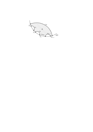
Figure 9. The disk $\Delta$.

Finally, we calculate the slope associated to the incompressible surface $S$. Since both of the tangles in $T_{1}$ have constant edgepaths, $\tau(S_{1})=0$. Since there are neither $0$ nor $\infty$ edges in the train track for $T_{1}$ and $c<0$, $\tau^{\prime}(S_{1})=2$. For $\tau(S_{2})$, there is one upward edge on $\mathcal{D}$ for the $-\frac{1}{n}$ tangle and there are a further $n^{2}+2n-1$ upward edges for the $\frac{1}{n+1}$ tangle, so $\tau(S_{2})=2(-1-(n^{2}+2n-1))=-2(n^{2}+2n)$. The twist of the surface is therefore $\tau(S)=-\tau(S_{1})+\tau^{\prime}(S_{1})+\tau(S_{2})=0+2-2(n^{2}+2n)=-2(n+1)^{2}+4$ by Lemma 4.5.

Let $S_{0,1}$ and $S_{0,2}$ be pieces of a Seifert surface $S_{0}$ for $T_{1}$ and $T_{2}$, respectively, obtained as in [5]. Since $S_{0,1}$ and $S_{0,2}$ are given by the same edgepaths, we have $\tau(S_{0})=-\tau(S_{0,1})+\tau(S_{0,2})=0$ by Lemma 4.4. Therefore the boundary slope of the incompressible surface $S$ is $\tau(S)-\tau(S_{0})=-2(n+1)^{2}+4$ by Lemma 4.5. ∎

Proof of Theorem 1.1.

As in Figure 7, $K_{n}$ has an irreducible alternating diagram with $4n$ crossings, so that $c(K_{n})=4n$. By Proposition 5.1, $\text{\rm diam}(K_{n})\geq 2(n+1)^{2}-4-(-2(n+1)^{2}+4)=4(n+1)^{2}-8$. Therefore, $\frac{\text{\rm diam}(K_{n})}{c(K_{n})}\geq\frac{(n+1)^{2}-2}{n}$ tends to infinity, as required. ∎

References

-
[1]
M. Culler, A table of A-polynomials computed via numerical methods.
http://www.math.uic.edu/~culler/
Apolynomials/ - [2] C. Curtis and S. Taylor, The Jones polynomial and boundary slopes of alternating knots. arXiv:0910.4912v3
- [3] N. Dunfield and S. Garoufalidis, Incompressibity criteria for spun-normal surfaces. Trans. Amer. Math. Soc. 364 (2012), 6109-6137.
- [4] A. Hatcher and W. Thurston, Incompressible surfaces in 2-bridge knot complements. Invent. Math. 79 (1985), 225–246.
- [5] A. Hatcher and U. Oertel, Boundary slopes for Montesinos knots. Topology 28 (1989), 453–480.
- [6] J. Howie, Boundary slopes of some non-Montesinos knots. arXiv:1401.2726
- [7] K. Ichihara and S. Mizushima, Crossing number and diameter of boundary slope set of Montesinos knot. Comm. Anal. Geom. 16 (2008), 565–589. arXiv:math/0510370
- [8] Y. Kabaya, Private communication, April, 2008.
- [9] Y. Kabaya, A method to find ideal points from ideal triangulations. J. Knot Theory Ramifications 19 (2010), 509–524. arXiv:0706.0971.
- [10] Y.-Q. Wu, Exceptional Dehn surgery on large arborescent knots. Pacific J. Math. 252 (2011), 219–243.