Synthetic Controls with Imperfect Pre-Treatment Fit

We analyze the properties of the Synthetic Control (SC) and related estimators when the pre-treatment fit is imperfect. In this framework, we show that these estimators are generally biased if treatment assignment is correlated with unobserved confounders, even when the number of pre-treatment periods goes to infinity. Still, we show that a demeaned version of the SC method can substantially improve in terms of bias and variance relative to the difference-in-difference estimator. We also derive a specification test for the demeaned SC estimator in this setting with imperfect pre-treatment fit. Given our theoretical results, we provide practical guidance for applied researchers on how to justify the use of such estimators in empirical applications.

Keywords: synthetic control; difference-in-differences; policy evaluation; linear factor model

JEL Codes: C13; C21; C23

1 Introduction

In a series of influential papers, Abadie and Gardeazabal (2003), Abadie et al. (2010), and Abadie et al. (2015) proposed the Synthetic Control (SC) method as an alternative to estimate treatment effects in comparative case studies when there is only one treated unit. The main idea of the SC method is to use the pre-treatment periods to estimate weights such that a weighted average of the control units reconstructs the pre-treatment outcomes of the treated unit, and then use these weights to compute the counterfactual of the treated unit in case it were not treated. According to Athey and Imbens (2017), “the simplicity of the idea, and the obvious improvement over the standard methods, have made this a widely used method in the short period of time since its inception”, making it “arguably the most important innovation in the policy evaluation literature in the last 15 years”. As one of the main advantages that helped popularize the method, Abadie et al. (2010) derive conditions under which the SC estimator would allow confounding unobserved characteristics with time-varying effects, as long as there exist weights such that a weighted average of the control units fits the outcomes of the treated unit for a long set of pre-intervention periods.

In this paper, we analyze the properties of the SC and related estimators when potential outcomes are determined by a linear factor model, which is the structure considered by Abadie et al. (2010) and Abadie (2020) to derive the main theoretical justifications for the SC estimator. Differently from Abadie et al. (2010), we consider the case in which the pre-treatment fit is imperfect. In a model with “non-diverging” common factors and a fixed number of control units ($J$), we show that the SC weights converge in probability to weights that do not, in general, reconstruct the factor loadings of the treated unit when the number of pre-treatment periods ($T_{0}$) goes to infinity. This happens because, in this setting, the SC weights converge to weights that simultaneously attempt to match the factor loadings of the treated unit and to minimize the variance of a linear combination of the idiosyncratic shocks. Therefore, weights that reconstruct the factor loadings of the treated unit are not generally the solution to this problem, even if such weights exist. While in many applications $T_{0}$ may not be large enough to justify large-$T_{0}$ asymptotics (e.g. Doudchenko and Imbens (2016)), our results can also be interpreted as the SC weights not converging to weights that reconstruct the factor loadings of the treated unit even when $T_{0}$ is large.

As a consequence, the SC estimator is biased if treatment assignment is correlated with the unobserved heterogeneity in this setting, even when the number of pre-treatment periods goes to infinity. The intuition is the following: if treatment assignment is correlated with common factors in the post-treatment periods, then we would need a SC unit that is affected in exactly the same way by these common factors as the treated unit, but did not receive the treatment, to obtain an unbiased estimator. However, this condition is not attained when the pre-treatment fit is imperfect, even when $T_{0}$ is large. Our results are not as conflicting with the results from Abadie et al. (2010) as it might appear at first glance. The asymptotic bias of the SC estimator, in our framework, goes to zero when the variance of the idiosyncratic shocks is small. This is the case in which one should expect to have a close-to-perfect pre-treatment fit when $T_{0}$ is large, which is the setting the SC estimator was originally designed for. Our theory complements the theory developed by Abadie et al. (2010), by considering the properties of the SC estimator when the pre-treatment fit is imperfect.

One important implication of the SC restriction to convex combinations of the control units is that the SC estimator may be biased even if treatment assignment is only correlated with time-invariant unobserved variables, which is essentially the identification assumption of the difference-in-differences (DID) estimator. We therefore consider a modified SC estimator, where we demean the data using information from the pre-intervention period, and then construct the SC estimator using the demeaned data. An advantage of demeaning is that it is possible to, under some conditions, show that the SC estimator dominates the DID estimator in terms of variance and bias in this setting. Moreover, we provide a specification test for the validity of the demeaned SC estimator in this setting with an imperfect pre-treatment fit. Finally, we also show that, in a setting with both non-diverging and diverging common factors, diverging common shocks would not generate asymptotic bias in the demeaned SC estimator, but we need that treatment assignment is uncorrelated with the non-diverging common factors to guarantee asymptotic unbiasedness.

If potential outcomes follow a linear factor model structure, then it would be possible to construct a counterfactual for the treated unit if we could consistently estimate the factor loadings. However, with fixed $J$, it is only possible to estimate factor loadings consistently under strong assumptions on the idiosyncratic shocks (e.g., Bai (2003) and Anderson (1984)). Therefore, the asymptotic bias we find for the SC estimator is consistent with the results from a large literature on factor models. We show that the asymptotic bias we derive for the SC estimator also applies to other related panel data approaches that have been studied in the context of an imperfect pre-treatment fit, such as Hsiao et al. (2012), Li and Bell (2017), Carvalho et al. (2018), Carvalho et al. (2016), and Masini and Medeiros (2016), in settings with fixed $J$. We show that these papers rely on assumptions that implicitly imply no selection on unobservables, which clarifies why their consistency/unbiasedness results when $J$ is fixed are not conflicting with our main results.

Also consistent with the literature on factor models, if we impose restrictions on the idiosyncratic shocks, then there are asymptotically unbiased alternatives. For example, Amjad et al. (2017) propose a de-noising algorithm, but it relies on idiosyncratic errors being serially uncorrelated. However, this may not be an appealing assumption in common applications. To the best of our knowledge, there is no estimator that is asymptotically valid in settings with fixed $J$ without assuming such kind of additional assumptions. Finally, Powell (2017) proposes a 2-step estimation in a setting with fixed $J$ in which the SC unit is constructed based on the fitted values of the outcomes on unit-specific time trends. However, we show that the demeaned SC method is already very efficient in controlling for polynomial time trends

When both $J$ and $T_{0}$ diverge, Gobillon and Magnac (2016), Xu (2017), Athey et al. (2017), and Arkhangelsky et al. (2018) provide alternative estimation methods that are asymptotically valid when the number of both pre-treatment periods and controls increase. This is also consistent with the literature on linear factor models, which shows that these models can be consistently estimated in large panels (e.g., Bai (2003), Bai and Ng (2002), Bai (2009), and Moon and Weidner (2015)). Ferman (2019) provides conditions under which the original and the demeaned SC estimators are also asymptotically unbiased in this setting with large $J$/large $T_{0}$. The main requirement is that, as the number of control units increases, there are weights diluted among an increasing number of control units that recover the factor loadings of the treated unit. In contrast, our results on the bias of the SC estimator provide a better approximation for the properties of the SC estimator for cases in which this condition on the weights is not valid, and/or when $J$ and $T_{0}$ are roughly of the same size, but they are not large enough, so that a large $T_{0}$/large $J$ asymptotics does not provide a good approximation.

The remainder of this paper proceeds as follows. In Section 2 we describe our setting and provide a brief review of the SC estimator. The main results are presented in Section 3. We then present a Monte Carlo (MC) simulation in Section 4, and an empirical illustration in Section 5. In Section 6 we provide a guideline for applied researchers on how to justify the use of the SC method, based on our theoretical results. We conclude in Section 7.

2 Base Model

Suppose we have a balanced panel of $J+1$ units indexed by $j=0,...,J$ observed on a total of $T$ periods. We want to estimate the treatment effect of a policy change that affected only unit $j=0$, and we have information before and after the policy change. Let $\mathcal{T}_{0}$ ($\mathcal{T}_{1}$) be the set of time indices in the pre-treatment (post-treatment) periods. We assume that potential outcomes follow a linear factor model.

Assumption 1 (potential outcomes)

Potential outcomes when unit $j$ at time $t$ is treated ($y_{jt}^{I}$) and non-treated ($y_{jt}^{N}$) are given by

$$\begin{cases}y_{jt}^{N}=c_{j}+\delta_{t}+\lambda_{t}\mu_{j}+\epsilon_{jt}\\ y_{jt}^{I}=\alpha_{jt}+y_{jt}^{N},\end{cases}$$ (1)

where $\delta_{t}$ is an unknown common factor with constant factor loadings across units, $c_{j}$ is an unknown time-invariant fixed effect, $\lambda_{t}$ is a $(1\times F)$ vector of common factors, $\mu_{j}$ is a $(F\times 1)$ vector of unknown factor loadings, and the error terms $\epsilon_{jt}$ are unobserved idiosyncratic shocks.

In principle, the terms $\delta_{t}$ and $c_{j}$ could be included in the linear factor structure $\lambda_{t}\mu_{j}$. We include these separately because we want to consider $\lambda_{t}$ as a vector of common factors that do not have constant effects across units and that do not include a time-invariant fixed effect. Therefore, we can think of $\lambda_{t}$ as time-varying unobservables that may affect different units differently. In order to simplify the exposition of our main results, we consider the model without observed covariates $Z_{j}$. In Appendix Section A.5.2 we consider the model with covariates.

The treatment effect on unit $j$ at time $t$ is given by $\alpha_{jt}$, and the main goal of the SC method is to estimate the effect of the treatment for unit 0 for each post-treatment $t$, that is $\{\alpha_{1t}\}_{t\in\mathcal{T}_{1}}$. However, we only observe $y_{jt}=d_{jt}y_{jt}^{I}+(1-d_{jt})y_{jt}^{N}$, where $d_{jt}=1$ if unit $j$ is treated at time $t$.

We treat the vector of unknown factor loadings ($\mu_{j}$) and the treatment assignment as fixed, and consider the properties of the SC estimator under a repeated sampling framework over the distributions of the common factors ($\lambda_{t}$) and of the idiosyncratic shocks ($\epsilon_{jt}$). Alternatively, we can think that we have an underlying model where treatment assignment, $\mu_{j}$, $\lambda_{t}$, and $\epsilon_{jt}$ are stochastic, but we are conditioning on the treatment assignment and on the factor loadings. Assumption 2 defines the observed sample.

Assumption 2 (sampling)

We observe a realization of $\{y_{0t},...,y_{Jt}\}_{t\in\mathcal{T}_{0}\cup\mathcal{T}_{1}}$, where $y_{jt}=d_{jt}y_{jt}^{I}+(1-d_{jt})y_{jt}^{N}$, while $d_{jt}=1$ if $j=0$ and $t\in\mathcal{T}_{1}$, and zero otherwise. Potential outcomes are determined by equation (1). We treat $\{c_{j},\mu_{j}\}_{j=0}^{J}$ as fixed, and $\{\lambda_{t}\}_{t\in\mathcal{T}_{0}\cup\mathcal{T}_{1}}$ and $\{\epsilon_{jt}\}_{t\in\mathcal{T}_{0}\cup\mathcal{T}_{1}}$ for $j=0,...,J$ as stochastic.

In the assumption below we consider the identification assumption usually considered in the SC literature.

Assumption 3 (idiosyncratic shocks)

$\mathbb{E}[\epsilon_{jt}]=0$ for all $j\in\{0,1,...,J\}$ and $t\in\mathcal{T}_{1}\cup\mathcal{T}_{0}$.

Assumption 3, combined with the fact that we consider treatment assignment and factor loadings as fixed, compose the main restrictions we impose on the treatment assignment mechanism. It is easier to think about the assignment mechanism if we consider an underlying model in which treatment assignment and factor loadings are stochastic, and the expectation in Assumption 3 is conditional on the realization of these variables. In this case, Assumption 3 implies that idiosyncratic shocks are mean-independent from the treatment assignment. However, it does not impose any restriction on the dependence between treatment assignment and the factor structure. In particular, Assumption 3 does not impose any restriction on the distribution of $\lambda_{t}$ for $t\in\mathcal{T}_{1}$. We refer to that as “selection on unobservables”, meaning that treatment assignment may be correlated with the factor structure, but is uncorrelated with the idiosyncratic shocks.

Let $\boldsymbol{\mu}\equiv[\mu_{1}\ldots\mu_{J}]^{\prime}$, $\mathbf{c}\equiv[c_{1}\ldots c_{J}]^{\prime}$, $\mathbf{y}_{t}\equiv(y_{1t},\ldots,y_{Jt})$ and $\boldsymbol{\epsilon}_{t}\equiv(\epsilon_{1t},\ldots,\epsilon_{Jt})$. Following the original SC papers, we start restricting to convex combinations of the control units, so we consider weights in $\Delta^{J-1}\equiv\{(w_{1},...,w_{J})\in\mathbb{R}^{J}|w_{j}\geq 0\mbox{ and }\sum_{j=1}^{J}w_{j}=1\}$. We define $\widetilde{\Phi}=\{\textbf{w}\in\Delta^{J-1}~{}|~{}\mu_{0}=\boldsymbol{\mu}^{\prime}\mathbf{w}\mbox{ and }c_{0}=\mathbf{c}^{\prime}\mathbf{w}\}$. Therefore, $\mathbf{w}\in\widetilde{\Phi}$ is such that a weighted average of the control units absorbs all time correlated shocks of unit 0, $\lambda_{t}\mu_{0}$, and also absorbs the time-invariant fixed effects. Assuming $\widetilde{\Phi}\neq\varnothing$, if we knew $\textbf{w}^{\ast}\in\widetilde{\Phi}$, then we could consider an infeasible SC estimator using these weights, $\hat{\alpha}_{0t}^{\ast}=y_{0t}-\mathbf{y}_{t}^{\prime}{\mathbf{w}^{\ast}}$. For a given $t\in\mathcal{T}_{1}$, we would have

$$\hat{\alpha}^{\ast}_{0t}=y_{0t}-\mathbf{y}_{t}^{\prime}\mathbf{w}^{\ast}=\alpha_{0t}+\left(\epsilon_{0t}-\boldsymbol{\epsilon}_{t}^{\prime}\mathbf{w}^{\ast}\right).$$ (2)

Therefore, under Assumption 3, $\mathbb{E}[\hat{\alpha}^{\ast}_{0t}]=\alpha_{0t}$, which implies that this infeasible SC estimator is unbiased. Intuitively, the infeasible SC estimator constructs a SC unit for the counterfactual of $y_{0t}$ that is affected in the same way as unit 0 by each of the common factors (that is, $\mu_{0}=\boldsymbol{\mu}^{\prime}\mathbf{w}^{\ast}$) and has the same time-invariant fixed effect ($c_{0}=\mathbf{c}^{\prime}\mathbf{w}^{\ast}$), but did not receive treatment. Therefore, the only difference between unit 0 and this SC unit, beyond the treatment effect, would be given by the idiosyncratic shocks, which are assumed to have mean zero (Assumption 3), implying that this infeasible SC estimator is unbiased.

It is important to note that Abadie et al. (2010) do note make any assumption on $\widetilde{\Phi}\neq\varnothing$. Instead, they consider that there is a set of weights $\widetilde{\mathbf{w}}^{\ast}\in\Delta^{J-1}$ that satisfies $y_{0t}=\mathbf{y}_{t}^{\prime}\widetilde{\mathbf{w}}^{\ast}$ for all $t\in\mathcal{T}_{0}$. We call the existence of such weights $\widetilde{\mathbf{w}}^{\ast}\in\Delta^{J-1}$ as a “perfect pre-treatment fit” condition. While subtle, this reflects a crucial difference between our setting and the setting considered in the original SC papers. Abadie et al. (2010) and Abadie et al. (2015) consider the properties of the SC estimator conditional on having a perfect pre-intervention fit. As stated by Abadie et al. (2015), they “do not recommend using this method when the pretreatment fit is poor or the number of pretreatment periods is small”.

Abadie et al. (2010) provide conditions under which existence of $\widetilde{\mathbf{w}}^{\ast}\in\Delta^{J-1}$ such that $y_{0t}=\mathbf{y}_{t}^{\prime}\widetilde{\mathbf{w}}^{\ast}$ for all $t\in\mathcal{T}_{0}$ (for large $T_{0}$) implies that $\mu_{0}\approx\boldsymbol{\mu}^{\prime}\widetilde{\mathbf{w}}^{\ast}$. In this case, the bias of the SC estimator would be bounded by a function that goes to zero when $T_{0}$ increases. We depart from the original SC setting in that we consider a setting with imperfect pre-treatment fit, meaning that we do not assume existence of $\widetilde{\mathbf{w}}^{\ast}\in\Delta^{J-1}$ such that $y_{0t}=\mathbf{y}_{t}^{\prime}\widetilde{\mathbf{w}}^{\ast}$ for all $t\in\mathcal{T}_{0}$. The motivation to analyze the SC method in our setting is that the SC estimator has been widely used even when the pre-treatment fit is poor. Therefore, it is important to understand the properties of the estimator in this setting. Moreover, we show that the estimator can provide important improvements relative to DID even when the fit is imperfect, although in this case we should be more careful about the conditions for unbiasedness.

In order to implement their method, Abadie et al. (2010) recommend a nested minimization problem using the pre-intervention data to estimate the SC weights. We focus on the case where one includes all pre-intervention outcome values as predictors. In this case, the nested optimization problem proposed by Abadie et al. (2010) simplifies to

$$\widehat{\textbf{w}}^{\mbox{\tiny SC}} = \underset{{\textbf{w}\in\Delta^{J-1}}}{\mbox{argmin}}\frac{1}{T_{0}}\sum_{t\in\mathcal{T}_{0}}\left[y_{0t}-\mathbf{y}_{t}^{\prime}\mathbf{w}\right]^{2}.$$ (3)

For a given $t\in\mathcal{T}_{1}$, the SC estimator is then defined by $\hat{\alpha}_{0t}=y_{0t}-\mathbf{y}_{t}^{\prime}\widehat{\mathbf{w}}^{\mbox{\tiny SC}}$. Ferman et al. (2020) provide conditions under which the SC estimator using all pre-treatment outcomes as predictors will be asymptotically equivalent, when $T_{0}\rightarrow\infty$, to any alternative SC estimator such that the number of pre-treatment outcomes used as predictors goes to infinity with $T_{0}$, even for specifications that include other covariates. Therefore, our results are also valid for these SC specifications under these conditions. In Appendix A.5 we also consider SC estimators using (1) the average of the pre-intervention outcomes as predictor, and (2) other time-invariant covariates in addition to the average of the pre-intervention outcomes as predictors.

3 Main results

We consider the asymptotic properties of the SC and alternative estimators when $T_{0}\rightarrow\infty$ and $J$ is fixed. As we discuss in Remark 2, our results are also relevant for the case in which $T_{0}$ is small. We consider the properties of the original SC estimator in Section 3.1 in a setting in which common factors are “non-diverging”, in the sense that the second moments of the pre-treatment averages of the common factors and of the idiosyncratic shocks converge in probability to non-stochastic constants. We propose and analyze a demeaned version of the SC estimator in Section 3.2 in this setting. Then we discuss in Section 3.3 a setting in which some common factors are “diverging”, in the sense that the variance of the idiosyncratic shocks become asymptotically irrelevant relative to the variance of the common shocks when $T_{0}$ increases. This setting is analyzed in more details in Appendix A.3.

3.1 Asymptotic bias of the original SC estimator

We consider a settings in which the pre-treatment averages of the first and second moments of the common factors and the idiosyncratic shocks converge in probability to non-stochastic constants. Importantly, note we do not require that the observed outcomes $y_{jt}$ satisfy these conditions, because we do not impose any restriction on $\delta_{t}$. We discuss in Section 3.3 the case in which diverging common shocks may have heterogeneous effects across units. Let $\varepsilon_{t}=(\epsilon_{0t},...,\epsilon_{Jt})$.

Assumption 4 (common and idiosyncratic shocks)

$\frac{1}{T_{0}}\sum_{t\in\mathcal{T}_{0}}\lambda_{t}\buildrel p\over{\rightarrow}0$, $\frac{1}{T_{0}}\sum_{t\in\mathcal{T}_{0}}\varepsilon_{t}\buildrel p\over{\rightarrow}0$,
$\frac{1}{T_{0}}\sum_{t\in\mathcal{T}_{0}}\lambda_{t}^{\prime}\lambda_{t}\buildrel p\over{\rightarrow}\Omega_{0}$ positive semi-definite, $\frac{1}{T_{0}}\sum_{t\in\mathcal{T}_{0}}\varepsilon_{t}\varepsilon_{t}^{\prime}\buildrel p\over{\rightarrow}\sigma^{2}_{\epsilon}I_{J+1}$, and $\frac{1}{T_{0}}\sum_{t\in\mathcal{T}_{0}}\varepsilon_{t}\lambda_{t}\buildrel p\over{\rightarrow}0$ when $T_{0}\rightarrow\infty$.

Assumption 4 allows for serial correlation for both idiosyncratic shocks and common factors. The only restriction on the serial correlation is that we can apply a law of large numbers so that these pre-treatment averages converge in probability. We assume $\frac{1}{T_{0}}\sum_{t\in\mathcal{T}_{0}}\varepsilon_{t}\varepsilon_{t}^{\prime}\buildrel p\over{\rightarrow}\sigma^{2}_{\epsilon}I_{J+1}$ in order to simplify the exposition of our results. However, this can be easily replaced by $\frac{1}{T_{0}}\sum_{t\in\mathcal{T}_{0}}\varepsilon_{t}\varepsilon_{t}^{\prime}\buildrel p\over{\rightarrow}\Sigma$ for any symmetric positive definite $(J+1)\times(J+1)$ matrix $\Sigma$, so that idiosyncratic shocks may be heteroskedastic and correlated across $j$. Assuming that $\frac{1}{T_{0}}\sum_{t\in\mathcal{T}_{0}}\lambda_{t}\buildrel p\over{\rightarrow}\omega_{0}$, setting $\omega_{0}=0$ is without loss of generality. Assumption 4 would be satisfied if, for example, $(\varepsilon^{\prime}_{t},\lambda_{t})$ is $\alpha-$mixing with exponential speed, with uniformly bounded fourth moments in the pre-treatment period, and $\varepsilon_{t}$ and $\lambda_{t}$ are independent. Note that this would allow the distribution of $\lambda_{t}$ to be different when we consider pre-treatment periods closer to the assignment of the treatment. In this case, $\lambda_{t}$ would not be stationary, but Assumption 4 would still hold. Finally, note that we do not impose any restriction on $\delta_{t}$.

We consider in Proposition 1 the asymptotic distributions of the original SC in this setting.

Proposition 1

Under Assumptions 1 to 4, $\mathbf{\widehat{w}}^{\mbox{\tiny SC}}\buildrel p\over{\rightarrow}\mathbf{\bar{w}}$ when $T_{0}\rightarrow\infty$, where $(c_{0},\mu_{0})\neq(\mathbf{c}^{\prime}\mathbf{\bar{w}},\boldsymbol{\mu}^{\prime}\mathbf{\bar{w}})$, unless $\sigma_{\epsilon}^{2}=0$ or $\exists\textbf{w}\in\widetilde{\Phi}|\textbf{w}\in\underset{{\textbf{w}\in\Delta^{J-1}}}{\mbox{argmin}}\left\{\mathbf{w}^{\prime}\mathbf{w}\right\}$. Moreover, for $t\in\mathcal{T}_{1}$,

$$\hat{\alpha}_{0t}=y_{0t}-\mathbf{y}_{t}^{\prime}\widehat{\mathbf{w}}^{\mbox{\tiny SC}}\buildrel p\over{\rightarrow}\alpha_{0t}+\lambda_{t}\left(\mu_{0}-\boldsymbol{\mu}^{\prime}\mathbf{\bar{w}}\right)+\left(c_{0}-\mathbf{c}^{\prime}\mathbf{\bar{w}}\right)+\left(\epsilon_{0t}-\boldsymbol{\epsilon}_{t}^{\prime}\mathbf{\bar{w}}\right)\mbox{ when }T_{0}\rightarrow\infty.$$ (4)

Proposition 1 shows that the weights of the original SC estimators will generally not converge to weights that recover the factor loadings of the treated unit. The intuition is that $\mathbf{\widehat{w}}^{\mbox{\tiny SC}}$ converges in probability to $\mathbf{w}\in\Delta^{J-1}$ that minimizes the probability limit of equation (3), which is given by

$$Q_{0}(\mathbf{w})=\left[\left(c_{0}-\mathbf{c}^{\prime}\mathbf{w}\right)^{2}+\left(\mu_{0}-\boldsymbol{\mu}^{\prime}\mathbf{w}\right)^{\prime}\Omega_{0}\left(\mu_{0}-\boldsymbol{\mu}^{\prime}\mathbf{w}\right)\right]+\sigma_{\epsilon}^{2}\left(1+\mathbf{w}^{\prime}\mathbf{w}\right).$$ (5)

This objective function has two parts. The first one reflects the presence of common factors $\lambda_{t}$ and differences in the fixed effects that remain after we choose the weights to construct the SC unit. If $\widetilde{\Phi}\neq\varnothing$, then we can set this part equal to zero by choosing $\textbf{w}^{\ast}\in\widetilde{\Phi}$. However, this objective function also depends on the variance of a weighted average of the idiosyncratic shocks $\epsilon_{jt}$, implying that choosing $\textbf{w}^{\ast}\in\widetilde{\Phi}$ will not generally be the solution to this problem. As a consequence, the SC weights will generally converge to weights that do not recover the factor loadings of the treated unit, even if $\widetilde{\Phi}\neq\varnothing$. The SC weights would only asymptotically recover the factor loadings of the treated unit if $\sigma_{\epsilon}^{2}=0$ or $\exists\textbf{w}\in\widetilde{\Phi}\mbox{ such that }\textbf{w}\in\mbox{argmin}_{\textbf{w}\in\Delta^{J-1}}\left\{\mathbf{w}^{\prime}\mathbf{w}\right\}$. Given this rationale, such distortion on the SC weights will tend to be smaller when the common trends are much stronger than the idiosyncratic shocks (so that the second part of the objective function $Q_{0}(\mathbf{w})$ becomes less relevant). We present details of proof in Appendix A.1.1. Another intuition for this result is that the outcomes of the controls work as proxy variables for the factor loadings of the treated unit, but they are measured with error. We present this interpretation in more detail in Appendix A.2.

Proposition 1 also shows that the SC estimator converges in probability to the parameter we want to estimate ($\alpha_{0t}$) plus linear combinations of contemporaneous idiosyncratic shocks and common factors. By Assumption 3, $\mathbb{E}[\epsilon_{jt}]=0$, so whether this estimator is asymptotically unbiased depends crucially on the differences in how the treated and the SC units are affected by the common shocks, $\lambda_{t}\left(\mu_{0}-\boldsymbol{\mu}^{\prime}\mathbf{\bar{w}}\right)$, and on whether the SC unit reconstructs $c_{0}$. We can guarantee asymptotic unbiasedness for the original SC estimator if we assume that, for $t\in\mathcal{T}_{1}$, $\mathbb{E}\left[\lambda^{k}_{t}\right]=0$ for all common factors $k$ such that $\mu^{k}_{0}\neq\sum_{j\neq 0}\bar{w}_{j}^{\mbox{\tiny SC}}\mu^{k}_{j}$, and $c_{0}=\mathbf{c}^{\prime}\mathbf{w}$. Therefore, once we relax the perfect fit condition, Assumption 3, which allows for selection on unobservables, is not sufficient to guarantee that the SC estimator is asymptotically unbiased. More specifically, Proposition 1 shows that, once we relax the perfect fit condition, the original SC estimator will generally be asymptotically biased when treatment assignment is correlated with time-varying unobservables, and when the SC weights fail to recover the levels of the treated unit. This second conclusion implies that the SC estimator may be biased even when a DID estimator would be unbiased.

Remark 1

The discrepancy of our results with the results from Abadie et al. (2010) arises because we consider different frameworks. Abadie et al. (2010) consider the properties of the SC estimator conditional on having a perfect pre-treatment fit. Our results are not as conflicting with the results from Abadie et al. (2010) as they may appear at first glance. In a model with non-diverging common factors, the probability that one has a dataset at hand such that the SC weights provide a close-to-perfect pre-intervention fit with a moderate $T_{0}$ is close to zero, unless the variance of the idiosyncratic shocks is small. Therefore, our results agree with the theoretical results from Abadie et al. (2010) in that the asymptotic bias of the SC estimator should be small in situations where one would expect to have a close-to-perfect fit for a large $T_{0}$.

Remark 2

While many SC applications do not have a large number of pre-treatment periods to justify large-$T_{0}$ asymptotics (see, for example, Doudchenko and Imbens (2016)), our results can also be interpreted as the SC weights not converging to weights that reconstruct the factor loadings of the treated unit when $J$ is fixed even when $T_{0}$ is large. In Appendix A.2, we show that the problem we present remains if we consider a setting with finite $T_{0}$.

Remark 3

Related to Remark 2, the bias we derive for the SC estimator does not come from the difficulty in having a perfect pre-treatment fit when $T_{0}$ is large and $J$ is fixed. Rather, this would remain a problem when $J$ is fixed, even if $T_{0}$ is small enough so that a perfect pre-treatment fit is achieved due to over-fitting.

Remark 4

Having a larger $T_{0}$ could make the problem worse if the linear factor model for the post-treatment periods does not approximate well the potential outcomes in earlier periods. For example, imagine we have $y^{N}_{jt}=\lambda_{t}\mu_{j}+\epsilon_{jt}$ for the post-treatment periods and for the $M$ periods before the treatment, and $y^{N}_{jt}=\lambda_{t}\tilde{\mu}_{j}+\epsilon_{jt}$ for earlier periods, with $\mu_{j}$ potentially different from $\tilde{\mu}_{j}$. In this case, including more pre-treatment periods would likely induce more bias in the SC estimator, because in this case the first part of the objective function in (5) would be minimized with a $\widetilde{\mathbf{w}}$ such that $\mu_{0}\neq\boldsymbol{\mu}^{\prime}\widetilde{\mathbf{w}}$. In any case, our results from Proposition 1 should be interpreted as the SC estimator generally being asymptotically biased if there is selection on unobservables even when $T_{0}\rightarrow\infty$ and the factor loadings are stable for all periods when $T_{0}\rightarrow\infty$.

3.2 Comparison with DID estimator & the demeaned SC estimator

In contrast to the SC estimator, the DID estimator for the treatment effect in a given post-intervention period $t\in\mathcal{T}_{1}$ would be given by

$$\hat{\alpha}^{\tiny DID}_{0t} = y_{0t}-\frac{1}{J}\mathbf{y}_{t}^{\prime}\mathbf{i}-\frac{1}{T_{0}}\sum_{\tau\in\mathcal{T}_{0}}\left[y_{0\tau}-\frac{1}{J}\mathbf{y}_{\tau}^{\prime}\mathbf{i}\right],$$ (6)

where $\mathbf{i}$ is a $J\times 1$ vector of ones. Under Assumptions 1, 2, and 4, we have that

$$\hat{\alpha}^{\tiny DID}_{0t} \buildrel p\over{\rightarrow} \alpha_{0t}+\left(\epsilon_{0t}-\frac{1}{J}\boldsymbol{\epsilon}_{t}^{\prime}\mathbf{i}\right)+\lambda_{t}\left(\mu_{0}-\frac{1}{J}\boldsymbol{\mu}^{\prime}\mathbf{i}\right)\mbox{ when }T_{0}\rightarrow\infty.$$ (7)

Therefore, the DID estimator will be asymptotically unbiased in this setting if $\mathbb{E}[\lambda_{t}]=0$ for the factors such that $\mu_{0}\neq\frac{1}{J}\boldsymbol{\mu}^{\prime}\mathbf{i}$. This would be the case if treatment assignment is uncorrelated with the time-varying common factors. Differently from the SC estimator, however, the DID estimator would not be biased if the average of the control units do not recover the fixed effect of the treated unit.

As an alternative to the standard SC estimator, we suggest a modification in which we calculate the pre-treatment average for all units and demean the data. This is equivalent to a generalization of the SC method suggested, in parallel to our paper, by Doudchenko and Imbens (2016), which includes an intercept parameter in the minimization problem to estimate the SC weights and construct the counterfactual. Here we formally consider the implications of this alternative on the bias and variance of the SC estimator.

The demeaned SC estimator is given by $\hat{\alpha}^{\mbox{\tiny SC${}^{\prime}$}}_{0t}=y_{0t}-\mathbf{y}_{t}^{\prime}\widehat{\mathbf{w}}^{\mbox{\tiny SC${}^{\prime}$}}-(\bar{y}_{0}-\mathbf{\bar{y}}^{\prime}\widehat{\mathbf{w}}^{\mbox{\tiny SC${}^{\prime}$}})$, where $\bar{y}_{0}$ is the pre-treatment average of unit $0$, and $\mathbf{\bar{y}}$ is an $J\times 1$ vector with the pre-treatment averages of the controls. We define $\Phi=\{\textbf{w}\in\Delta^{J-1}~{}|~{}\mu_{0}=\boldsymbol{\mu}^{\prime}\mathbf{w}\}$. In this case, the weights $\widehat{\textbf{w}}^{\mbox{\tiny SC${}^{\prime}$}}$ are given by

$$\widehat{\textbf{w}}^{\mbox{\tiny SC${}^{\prime}$}}=\underset{{\textbf{w}\in\Delta^{J-1}}}{\mbox{argmin}}\frac{1}{T_{0}}\sum_{t\in\mathcal{T}_{0}}\left[y_{0t}-\mathbf{y}_{t}^{\prime}\mathbf{w}-\left(\bar{y}_{0}-\mathbf{\bar{y}}^{\prime}\mathbf{w}\right)\right]^{2}.$$ (8)

Proposition 2

Under Assumptions 1, 2, 3 and 4, $\widehat{\textbf{w}}^{\mbox{\tiny SC${}^{\prime}$}}\buildrel p\over{\rightarrow}\mathbf{\bar{w}}^{\mbox{\tiny SC${}^{\prime}$}}$ when $T_{0}\rightarrow\infty$, where $\mu_{0}\neq\boldsymbol{\mu}^{\prime}\mathbf{\bar{w}}^{\mbox{\tiny SC${}^{\prime}$}}$, unless $\sigma_{\epsilon}^{2}=0$ or $\exists\textbf{w}\in\Phi|\textbf{w}\in\underset{{\textbf{w}\in\Delta^{J-1}}}{\mbox{argmin}}\left\{\mathbf{w}^{\prime}\mathbf{w}\right\}$. Moreover, for $t\in\mathcal{T}_{1}$,

$$\hat{\alpha}^{\mbox{\tiny SC${}^{\prime}$}}_{0t}\buildrel p\over{\rightarrow}\alpha_{0t}+\left(\epsilon_{0t}-\boldsymbol{\epsilon}_{t}^{\prime}\mathbf{\bar{w}}^{\mbox{\tiny SC${}^{\prime}$}}\right)+\lambda_{t}\left(\mu_{0}-\boldsymbol{\mu}^{\prime}\mathbf{\bar{w}}^{\mbox{\tiny SC${}^{\prime}$}}\right)\mbox{ when }T_{0}\rightarrow\infty.$$ (9)

Therefore, both the demeaned SC and the DID estimators are asymptotically unbiased when $\mathbb{E}[\lambda_{t}]=0$ for $t\in\mathcal{T}_{1}$. Differently from the original SC estimator, these estimators do not require that the weights recover the fixed effect of the treated unit for unbiasedness. The proof is essentially the same as the one for Proposition 1 (details in Appendix A.1.2).

With additional assumptions on $(\epsilon_{0t},...,\epsilon_{Jt},\lambda_{t}^{\prime})$ in the post-treatment periods, we can also assure that the demeaned SC estimator is asymptotically more efficient than DID.

Assumption 5 (Stability in the pre- and post-treatment periods)

For $t\in\mathcal{T}_{1}$, $\mathbb{E}[\lambda_{t}]=0$, $\mathbb{E}[\epsilon_{t}]=0$, $\mathbb{E}[\lambda_{t}^{\prime}\lambda_{t}]=\Omega_{0}$, and $\mathbb{E}[\epsilon_{t}\epsilon_{t}^{\prime}]=\sigma^{2}_{\epsilon}I_{J+1}$, $cov(\epsilon_{t},\lambda_{t})=0$.

Assumptions 4 and 5 imply that idiosyncratic shocks and common factors have the same first and second moments in the pre- and post-treatment periods. Again, the assumptions that idiosyncratic errors are homoskedastic is made just for simplification. What is crucial in this assumption is that the variance/covariance matrix of the idiosyncratic shocks in the post-treatment periods is the same as the long-run variance/covariance matrix of the idiosyncratic shocks in the pre-treatment periods. From Proposition 2, Assumption 5 implies that the demeaned SC estimator is asymptotically unbiased. We now show that this assumption also implies that the demeaned SC estimator has lower asymptotic MSE than the DID estimator.

Proposition 3

Under Assumptions 1 to 5, the demeaned SC estimator ($\hat{\alpha}^{\mbox{\tiny SC${}^{\prime}$}}_{0t}$) dominates the DID estimator ($\hat{\alpha}^{\tiny DID}_{0t}$) in terms of asymptotic MSE when $T_{0}\rightarrow\infty$.

The intuition of this result is that, under Assumption 5, the demeaned SC weights converge to weights that minimize a function $\Gamma(\mathbf{w})$ such that $\Gamma(\mathbf{\bar{w}}^{\mbox{\tiny SC${}^{\prime}$}})=a.var(\hat{\alpha}^{\mbox{\tiny SC${}^{\prime}$}}_{0t})$, and $\Gamma(\{\frac{1}{J},...,\frac{1}{J}\})=a.var(\hat{\alpha}^{\mbox{ \tiny DID}}_{1t})$. Therefore, it must be that the asymptotic variance of $\hat{\alpha}^{\mbox{\tiny SC${}^{\prime}$}}_{0t}$ is weakly lower than the variance of $\hat{\alpha}^{\mbox{ \tiny DID}}_{1t}$. Moreover, these estimators are unbiased under these assumptions (details in Appendix A.1.3).

If we had that $\mathbb{E}[\lambda_{t}]\neq 0$ for $t\in\mathcal{T}_{1}$, then both the demeaned SC and the DID estimators would generally be asymptotically biased. In general, it is not possible to rank the demeaned SC and the DID estimators in terms of bias and MSE if treatment assignment is correlated with time-varying common factors. We provide in Appendix A.4 a specific example in which the DID can have a smaller bias and MSE relative to the demeaned SC estimator. This might happen when selection into treatment depends on common factors with low variance, and it happens that a simple average of the controls provides a good match for the factor loadings associated with these common factors. In general, however, we should expect a lower bias for the demeaned SC estimator, given that the demeaned SC weights are partially chosen to minimize the distance between $\mu_{0}$ and $\boldsymbol{\mu}^{\prime}\widehat{\textbf{w}}^{\mbox{\tiny SC${}^{\prime}$}}$, while the DID estimator uses weights that are not data driven.

Since the biases of these two estimators would generally differ when $\mathbb{E}[\lambda_{t}]\neq 0$ for $t\in\mathcal{T}_{1}$, we can consider a specification test by contrasting these two estimators. More specifically, if the DID estimator is very different from the demeaned SC estimator, this would suggest that both estimators are biased (considering the setting in which the pre-treatment fit is imperfect).

A potential problem in properly testing the equality of these two estimators is that they are generally not asymptotically normal. Still, if we consider a stronger assumption that $\lambda_{t}$ and $\epsilon_{jt}$ are stationary and weakly dependent for all $t\in\mathcal{T}_{0}\cup\mathcal{T}_{1}$, which implies that $\mathbb{E}[\lambda_{t}]=0$ for $t\in\mathcal{T}_{1}$, then we can follow the idea from Chernozhukov et al. (2017) and test this condition using in-time placebos. More specifically, let $\widetilde{\mathbf{w}}$ be the demeaned SC weights using all periods. We consider

$$\hat{u}_{t}=\left(\widetilde{\mathbf{w}}^{\prime}\mathbf{y}_{t}+\frac{1}{T_{0}+T_{1}}\sum_{\tau\in\mathcal{T}_{0}\cup\mathcal{T}_{1}}(y_{0\tau}-\widetilde{\mathbf{w}}^{\prime}\mathbf{y}_{\tau})\right)-\left(J^{-1}\mathbf{i}^{\prime}\mathbf{y}_{t}+\frac{1}{T_{0}+T_{1}}\sum_{\tau\in\mathcal{T}_{0}\cup\mathcal{T}_{1}}(y_{0\tau}-J^{-1}\mathbf{i}^{\prime}\mathbf{y}_{\tau})\right).$$ (10)

Following Chernozhukov et al. (2017), we impose the null $\mathbb{E}[\lambda_{t}]=0$ for $t\in\mathcal{T}_{1}$ and estimate the model using all periods of data to provide better finite sample properties.

The main idea is that, under the null that $\lambda_{t}$ and $\epsilon_{jt}$ are stationary and weakly dependent, $\hat{u}_{t}$ will approximately be stationary and weakly dependent. Therefore, we can construct a test statistic $S(\widehat{\mathbf{u}})=\left|\frac{1}{T_{1}}\sum_{t\in\mathcal{T}_{1}}\hat{u}_{t}\right|$, and derive the distribution of the test statistic by considering the set of all moving block permutations of the time periods. Let $\mathcal{T}_{0}=\{1,...,T_{0}\}$ and $\mathcal{T}_{1}=\{T_{0}+1,...,T\}$, and let $\Pi$ be the set of permutations $\pi_{j}$ indexed by $j\in{0,...,T-1}$ such that

$$\pi_{j}(i)=\begin{cases}i+j&\mbox{ if }i+j\leq T\\ i+j-T&\mbox{otherwise}.\end{cases}$$ (11)

Then the p-value of the specification test is given by

$$\hat{p}=\frac{1}{T}\sum_{j=0}^{T-1}\mathbf{1}\left\{S(\widehat{\mathbf{u}})>S(\widehat{\mathbf{u}}_{\pi_{j}})\right\},$$ (12)

We formalize this idea in the following proposition.

Proposition 4

Assume $\lambda_{t}$ and $\epsilon_{jt}$ are stationary and weakly dependent, with finite second moments, and that Assumptions 1 and 2 hold. Then, for any $a\in(0,1)$, $Pr(\hat{p}\leq a)\rightarrow a$ when $T_{0}\rightarrow\infty$ and $T_{1}$ is fixed.

If we find a low $\hat{p}$, indicating that the DID and the demeaned SC estimators are significantly different, then this would be an indication that both estimators are biased (considering the case in which the pre-treatment fit is imperfect). In contrast, a high $\hat{p}$ would provide some evidence that the condition $\mathbb{E}[\lambda_{t}]=0$ for $t\in\mathcal{T}_{1}$ is valid. If $\lambda_{t}$ and $\epsilon_{jt}$ are serially uncorrelated, then this test is exact. If there is serial correlation, though, then we may have distortions when $T_{0}$ is finite, but the test is asymptotically valid when $T_{0}\rightarrow\infty$.

Importantly, this test is completely uninformative about Assumption 3. Moreover, it relies on stationarity as an auxiliary assumption, which is not a necessary assumption for validity of the DID and the demeaned SC estimators in this setting. We also recommend applied researchers should plot the demeaned SC and the DID estimators to provide a visual inspection of the differences between these two estimators.

Remark 5

In general, it is not possible to compare the original and the demeaned SC estimators in terms of bias and variance. For example, if units with similar factor loadings also have similar fixed effects, then matching also on the levels would help provide a better approximation to $\mu_{0}$. Moreover, the demeaning process may increase the variance of the estimator for a finite $T_{0}$. Finally, demeaning essentially implies that we allow for extrapolation, which some may consider as one of the advantage of the SC estimator (e.g., Abadie et al. (2015)). Therefore, it is not clear whether demeaning is the best option in all applications, and the use of this estimator depends on the willingness of the researcher to allow for extrapolation.

Remark 6

Our main result that the original and the demeaned SC estimators are generally asymptotically biased if there are unobserved time-varying confounders (Propositions 1 and 2) still applies if we also relax the non-negative and the adding-up constraints, which essentially leads to the panel data approach suggested by Hsiao et al. (2012), and further explored by Li and Bell (2017). Our conditions for unbiasedness of the SC estimator also apply to the estimators proposed by Carvalho et al. (2018) and Carvalho et al. (2016) when $J$ is fixed. In Appendix A.5.3 we show that these papers rely on assumptions that implicitly imply that there is no selection on time-varying unobservables. This clarifies what selection on unobservables means in this setting, and reconciles our findings with the asymptotic unbiasedness/consistency results in these papers.

3.3 Model with “diverging” common factors

While the assumptions considered in Sections 3.1 and 3.2 allow for outcomes with divergent pre-treatment averages (which would be the case when we consider, for example, GDP or average wages), we restrict to settings in which such diverging common shocks affect all units in the same way. In Appendix A.3 we modify Assumption 1 to consider the case in which we may have diverging common shocks with heterogeneous effects across unit.

Assuming that there exist weights that reconstruct the factor loadings of the treated unit associated to the diverging common shocks, we show that the asymptotic distribution of the demeaned SC estimator does not depend on such diverging common shocks when $T_{0}\rightarrow\infty$. The intuition is that, as $T_{0}\rightarrow\infty$, the variance of a linear combination of the idiosyncratic shocks becomes irrelevant relative to the cost of failing to recover the factor loadings associated with the diverging common shocks. This is consistent with the conclusion from Section 3.1 that the bias of the SC estimator should be less relevant when the common shocks are stronger relative to the idiosyncratic shocks. However, if we also have non-diverging common shocks, then the demeaned SC weights will generally not asymptotically recover the factor loadings of the treated unit associated with those non-diverging shocks. This implies that the demeaned SC estimator may be asymptotically biased if there is correlation between treatment assignment and these non-diverging shocks, for exactly the same reasons outlined in Section 3.1.

We also show that the conclusion that the demeaned SC estimator does not depend on the diverging common shocks is not valid for the original SC estimator. While the SC weights considering the original SC method converge in probability to weights that recover the factor loadings of the treated associated to the diverging common shocks, this convergence may not be fast enough to compensate that such common shocks are diverging. We present all details on this setting in Appendix A.3.

4 Monte Carlo simulations

To illustrate our theoretical findings, we construct a MC simulation based on a real dataset using the monthly employment data for 50 US states and the District of Columbia ($J+1=51$) from January 1982 to December 2019 ($T=456$). We construct these series by aggregating the Current Population Survey (CPS) microdata at the state $\times$ month level. We estimate a factor model that best approximates this data. In addition to the state and time fixed effects, we estimate four common factors. We find evidence that these four factors and the 51 idiosyncratic shocks are stationary, suggesting that any non-stationary trends in the outcomes come from the time fixed effects, $\delta_{t}$. This provides evidence that this dataset is well approximated by the setting we consider in Sections 3.1 and 3.2. We consider state-specific Gaussian ARMA models for the distribution of each $\epsilon_{jt}$ and also for the distribution of the four common factors $\lambda_{t}$.

For each simulation, we fix the estimated factor loadings $\mu_{j}$ and consider random draws for $\lambda_{t}$ and $\epsilon_{jt}$ We set $T_{1}=12$ (one year) and $T_{0}\in\{120,240,480,1200\}$, and we vary which state is considered as treated. We consider $5000$ replications for each scenario. The case with $T_{0}=480$ have approximately the same number of pre-treatment periods as we have in our original dataset, while the cases with smaller $T_{0}$ reflect more common setting in which we have 10 or 20 years of pre-treatment data. We include the case $T_{0}=1200$ to approximate the asymptotic behavior of the estimators when $T_{0}\rightarrow\infty$.

We consider in Panels A and B of Table 1 the case in which $\mathbb{E}[\lambda_{t}]=0$ for $t\in\mathcal{T}_{1}$. In Panel A we consider that the treated state is such that $c_{0}$ is the second largest value in the distribution of $c_{j}$, while in Panel B the treated state has the second smallest value of $c_{0}$. We find that the original SC estimator is biased in both cases, even though it would be possible to have weights that reconstruct $c_{0}$. The problem is that such weights would be very concentrated on the state with largest (or smallest) $c_{j}$, so the SC weights would converge to weights that are more diluted, even if this means not recovering $c_{0}$. This is consistent with Proposition 1.

Figure 1.A shows the bias of the original SC estimator as a function of the state fixed effects of the treated unit. We find relevant bias of SC estimator when the fixed effects of the treated unit is in the extremes, while the bias is closer to zero when the treated unit is more in the middle of the distribution of the fixed effects. This happens because, as we consider a treated unit with fixed effects more towards the center of the distribution of fixed effects, we can have a weighted average of the control units with more diluted weights that reconstruct the fixed effects of the treated. Therefore, the term in equation 5 related to the variance of the linear combination of idiosyncratic shocks becomes less relevant in the minimization problem. Indeed, if we consider a measure of concentration of weights given by $||\mathbf{\widehat{w}}^{\mbox{\tiny SC}}||_{2}$, then the correlation between the absolute value of the bias of the SC estimator and this measure ranges from 0.723 to 0.849 (depending on the value of $T_{0}$).

Table 1: Monte Carlo Simulations

Bias Standard error SC Demeaned SC DID SC Demeaned SC DID (1) (2) (3) (4) (5) (6) Panel A: second largest $c_{j}$, no break $T_{0}=120$ 0.243 0.009 0.020 0.531 0.573 0.915 $T_{0}=240$ 0.200 -0.002 0.006 0.505 0.532 0.960 $T_{0}=480$ 0.196 0.006 0.007 0.501 0.514 1.007 $T_{0}=12000$ 0.167 -0.004 -0.010 0.503 0.500 1.005 Panel B: second smallest $c_{j}$, no break $T_{0}=120$ -0.565 0.020 0.028 1.173 0.823 1.368 $T_{0}=240$ -0.601 -0.012 0.002 1.242 0.801 1.431 $T_{0}=480$ -0.596 -0.011 0.004 1.264 0.755 1.469 $T_{0}=12000$ -0.581 -0.002 -0.003 1.242 0.714 1.442 Panel C: second largest $\mu_{1j}$, break in factor 1 $T_{0}=120$ 1.142 1.043 2.143 0.772 0.819 1.247 $T_{0}=240$ 0.934 0.797 2.129 0.728 0.764 1.308 $T_{0}=480$ 0.808 0.675 2.110 0.713 0.728 1.337 $T_{0}=12000$ 0.718 0.598 2.112 0.688 0.691 1.310 Panel D: second smallest $\mu_{1j}$, break in factor 1 $T_{0}=120$ -1.821 -1.851 -3.176 1.200 1.167 1.777 $T_{0}=240$ -1.573 -1.532 -3.157 1.130 1.113 1.794 $T_{0}=480$ -1.415 -1.324 -3.110 1.082 1.058 1.816 $T_{0}=12000$ -1.366 -1.230 -3.162 1.028 0.996 1.793
Notes: this table presents the MC simulations discussed in Section 4. Panels A and B consider the case in which all common factors have mean zero in the post-treatment periods. In Panel A, the treated unit is the state with second largest fixed effect in the distribution of $c_{j}$, while in Panel B the treated unit is the state with the second smallest fixed effect. Panels C and D consider the case in which the first common factor has expected value equal to two times its standard deviation in the post-treatment periods. In Panel C, the treated unit is the state with second largest factor loadings associated to the first common factor in the distribution of $\mu_{1j}$, while in Panel D the treated unit is the state with the second smallest factor loading. In all simulations, the true treatment effect is equal to zero.

Figure 1: Monte Carlo Simulations

2.A: Bias of original SC	2.B: Bias of demeaned SC

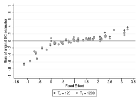
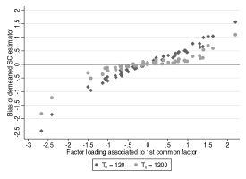
Notes: Figure A presents the bias of the original SC estimator as a function of the fixed effect of the treated state. We consider in this case a setting with no structural break for the common factors. Figure B presents the bias of the demeaned SC estimator as a function of the factor loadings associated to the first common factor of the treated state. We consider the case in which the first common factor has expected value equal to two times its standard deviation in the post-treatment periods. We present the settings with $T_{0}=120$ and $T_{0}=1200$. In all simulations, the true treatment effect is equal to zero.

In contrast to the original SC estimator, both the demeaned SC and the DID estimators are unbiased in this setting, as presented in Panel A of Table 1. This is consistent with Proposition 2. Moreover, as expected from Proposition 3, the demeaned SC estimator is more efficient than the DID estimator, with roughly 40%-50% smaller standard errors.

In Panels C and D of Table 1, we consider a setting in which the first common factor has expected value equal to two times its standard deviation in the post-treatment periods. In Panel C, we consider the case in which the treated state is such that $\mu_{10}$ is the second largest value in the distribution of $\mu_{1j}$, while in Panel D we consider the case in which it is the second smallest. Therefore, again we are in a setting in which it would be possible to construct a SC state that is affected by $\lambda_{1t}$ in the same way as the treated unit. Still, the results from columns 1 and 2 show that the original and the demeaned SC estimators are biased even when $T_{0}$ is large. This happens because the SC weights fail to reconstruct $\mu_{10}$, despite the fact that there exist weights that would do so. This is consistent with the results from Propositions 1 and 2. Note also that the biases of the original and demeaned SC estimators are larger when $T_{0}$ is smaller. See Ferman and Pinto (2019) for a more thorough discussion on that. Figure 1.B shows the bias of the demeaned SC estimator as a function of the factor loadings of the treated unit. Again, the bias is closer to zero when the treated unit is in the middle of the distribution of $\mu_{1j}$. If we consider a measure of concentration of weights given by $||\mathbf{\widehat{w}}^{\mbox{\tiny SC}^{\prime}}||_{2}$, then the correlation between the absolute value of the bias of the demeaned SC estimator and this measure ranges from 0.723 to 0.810 (depending on the value of $T_{0}$).

While the biases of the original and the demeaned SC estimators do not converge to zero when there is selection on unobservables, these biases are substantially smaller than the bias of the DID estimator in this setting (column 3). Interestingly, the bias of the demeaned SC estimator attenuates the bias from the DID estimator, but does not eliminate it. The idea is that, when we move from the DID to the demeaned SC estimator, the weights move in the direction of weights that reconstruct the factor loadings. However, the SC weights do not generally go all the way through to recover $\mu_{0}$ because of the idiosyncratic shocks. Moreover, the DID estimator presents a substantially larger standard error (columns 4 to 6). These results are consistent with the conclusions from Section 3.2, in that the demeaned SC estimator improves relative to DID in terms of bias and variance.

Finally, we consider the size and power of the specification test proposed in Section 3.2. We present in columns 1 to 4 of Appendix Table A.1 rejection rates when there is no structural break (so both the demeaned SC and the DID estimators are asymptotically unbiased), depending on the treated state and on $T_{0}$. The test presents relevant over-rejection when $T_{0}$ is small, but such distortions become less relevant when $T_{0}$ increases. Such distortions with finite $T_{0}$ arise because the common factors exhibit serial dependence. If we did not have dependence, then the test would be exact. Overall, the fact that the test has some over-rejection when $T_{0}$ is small is less worrisome than if we had under-rejection, because this would lead researchers to be more cautious about the use of the demeaned SC estimator. In columns 5 to 8, we consider the case in which there is a structural break. In this case, the test would have power to detect that the demeaned SC and the DID estimators are different, especially when the treated unit is on the extremes of the distribution of $\mu_{1j}$. When the treated unit is in the middle of this distribution, then the bias of both the demeaned SC and of the DID estimators become less relevant, so the probability of rejecting specification test becomes lower.

5 Empirical Illustration

As an empirical illustration, we revisit the application presented by Abadie and Gardeazabal (2003). We present in Figure 2.A the per capita GDP time series for the Basque Country and for other Spanish regions, while in Figure 2.B we replicate their Figure 1, which displays the per capita GDP of the Basque Country contrasted with the per capita GDP of a SC unit constructed to provide a counterfactual for the Basque Country without terrorism. We construct three different SC units, with the original SC estimator using all pre-treatment outcome lags as predictors, with the demeaned SC estimator using all pre-treatment outcome lags as predictors, and with the specification considered by Abadie and Gardeazabal (2003). All specifications point out to large negative treatment effects, although the estimated effects are slightly smaller for the original specifications considered by Abadie and Gardeazabal (2003).

Figure 2.B displays a remarkably good pre-treatment fit, regardless of the specification. However, the per capita GDP series are clearly non-stationary, with all regions displaying similar trends before the intervention. Considering the results presented in Section 3, such non-stationarity may come either from time fixed effects $\delta_{t}$, or from non-stationary common shocks that may have heterogeneous effects across regions. If the non-stationarity comes from a common factor $\delta_{t}$ that affects every unit in the same way, then the series $\tilde{y}_{jt}=y_{jt}-\frac{1}{J}\sum_{j^{\prime}\neq 0}y_{j^{\prime}t}$ would not display non-stationary trends. As shown in Figure 2.C, this appears to be the case in this application.

In light of the results from Section 3, the distortions in the SC weights depend on the relative magnitudes of the variance of the non-diverging common factors relative to the variance of the idiosyncratic shocks. Therefore, Figure 2.C provides a better visual assessment of whether the pre-treatment fit is good relative to Figure 2.B. While the pre-treatment fit is still reasonably good after we discard the non-stationary part of the series, it is not as good as when we consider the series in levels.

We can consider whether we would be able to justify the use of the SC method in this setting without relying on theoretical results based on perfect pre-treatment fit approximations. First, note that the estimated weights in this application are very concentrated among a few control regions, so we cannot rely on the theoretical results from Ferman (2019) to argue that the SC estimator is asymptotically unbiased in this setting (see Appendix Table A.2). Following the discussion in Section 3.2, we also contrast in Figure 2.D the DID and the demeaned SC estimators. If they were very similar, then we would have some support to rely on these estimators even if they failed to reconstruct the factor loadings of the treated region. However, we find the the estimated effect using the demeaned SC estimator is systematically larger. The p-value of the specification test proposed in Proposition 4 is $0.023$. This suggests that we may have selection on time-varying unobservables, implying that both the demeaned and the DID estimators are asymptotically biased, although the bias of the demeaned SC estimator should be smaller.

Figure 2: Abadie and Gardeazabal (2003) application

2.A: Raw data	2.B: GDP in level
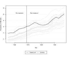
2.C: GDP de-trended	2.D: Demeaned SC vs DID estimators

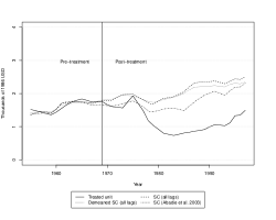
Notes: Figure A presents time series for the treated and for the control units used in the empirical application from Abadie and Gardeazabal (2003). In Figure B we present the time series for the treated and for the SC units. We consider the SC unit estimated with the original SC estimator using all pre-treatment periods lags, with the demeaned SC estimator using all pre-treatment periods lags, and with the specification considered by Abadie and Gardeazabal (2003). In Figure C we present the same information as in Figure B after subtracting the control groups’ averages for each time period. In Figure D we present the counterfactuals using the demeaned SC and the DID estimators.

Overall, since in this particular application the pre-treatment fit is reasonably good even once we subtract the non-stationary trends, and the treatment effects are large relative to the pre-treatment gaps, we should expect that any potential bias from the demeaned SC estimator does not explain a large proportion of the estimated effects. Moreover, given the discussions from Sections 3.2 and 4, we should expect the demeaned SC estimator to partially control for any bias that the DID estimator experience. Since the estimated effects with the demeaned SC estimator are stronger than the DID estimates, given this rationale, we should expect, if anything, that the demeaned SC estimator would provide a lower bound on the (absolute values of the) treatment effects. Therefore, a careful analysis of the potential problems of the SC method would not change the main conclusions from this empirical application. Still, in other settings in which the pre-treatment fit is worse, and in which moving from the DID to the demeaned SC estimator leads to weaker results, then it would not be possible to rely on the arguments used above, and the problems we highlight in this paper may undermine conclusions from the SC method.

6 Recommendations

Taken together, our results clarify the conditions in which the SC and related estimators can be reliably used, and provide guidance on how applied researchers could justify the use of these methods. First, a condition like the one we present in Assumption 3 is always necessary to justify the SC estimator. It states that treatment assignment is not related to shocks that are specific to the treated unit. It does allow, however, for unobserved confounders that may also affect other control units. Indeed, the main reason why a researcher should use these kind of methods is if he/she believes that there may be confounding factors that also affect the control units. In this case, information from the control units could be used to control for such confounders. Therefore, any applied paper relying on the SC method should discuss the possible unobserved confounders in the specific application, and argue that such confounders are not specific to the treated unit.

Importantly, even if it is plausible that idiosyncratic shocks are not correlated with the treatment assignment, whether the SC method is able to reliably control for the common shocks depends crucially on details of the empirical application. There are two settings that provide validity for the SC estimator even when there are time-varying unobserved confounders. First, Abadie et al. (2010) show that the SC estimator is reliable if the pre-treatment fit is good for a large number of pre-treatment periods. This condition can be checked by contrasting the outcomes of the treated and of the SC units in the pre-treatment periods. Based on our results, we recommend that applied researchers should also consider the pre-treatment fit after discarding diverging trends, in order to provide a better understanding of the relative magnitude between the variances of the non-diverging common factors and of the idiosyncratic shocks. Also, it is important that the number of control units in this case cannot be large in comparison to $T_{0}$, otherwise a good pre-treatment fit might be a consequence of over-fitting. In this case, the bias of the SC estimator we uncover in our paper may remain relevant even if we have a good pre-treatment fit.

Second, when both $J$ and $T_{0}$ are large, Ferman (2019) show that the SC estimator may be asymptotically unbiased even when the pre-treatment fit is imperfect. This would be the case if the confounders affect a large number of control units, and in this case the SC weights would get diluted among an increasing number of control units when $J\rightarrow\infty$. Therefore, we recommend that applied researchers also report the $L_{2}$ norm of the SC weights, $||\widehat{\textbf{w}}^{\mbox{\tiny SC}}||_{2}$. If this is close to zero, then we would have evidence that we are closer to the setting considered by Ferman (2019). In contrast, if the weights are concentrated, then we would have evidence that the bias we uncover in our paper is potentially relevant. As we show in our MC simulations in Section 4, the cases in which we find largest biases are exactly the ones in which the SC weights are more concentrated.

The results we derive in Section 3 are informative about the properties of the SC estimator when the conditions outlined by Abadie et al. (2010) and Ferman (2019) do not hold. This would be the case when (i) the pre-treatment fit is imperfect and $J$ is not large, (ii) the pre-treatment fit is imperfect with large $J$ and $T_{0}$, but the SC weights are not diluted among a large number of control units, or (iii) the pre-treatment fit is good, but $J$ is much larger than $T_{0}$, so such pre-treatment fit is possibly good due to over-fitting.

In these cases, we show that the SC estimator can still provide important gains relative to the DID estimator, but the applied researcher should be more careful in justifying the use of the method. If one considers the demeaned SC estimator, then the assumptions for unbiasedness would be the same as those for the DID estimator. That is, the researcher should argue that the relevant unobserved confounders are not time-varying. The advantage of relying on the demeaned SC estimator relative to DID in this case is that it would be more efficient if common shocks are stable before and after the treatment, and that it should have lower bias in case there is correlation between treatment assignment and time-varying unobservables. We also show that contrasting the DID and the demeaned SC estimators is informative about whether these conditions for unbiasedness are valid, and propose a specification test based on that. If we find evidence that these two estimators are similar, then we should be more confident that the conditions for asymptotic unbiasedness of the demeaned SC estimator holds even when we are not in the settings considered by Abadie et al. (2010) or Ferman (2019).

Importantly, if the conditions considered by Abadie et al. (2010) or Ferman (2019) hold in a specific application, then the demeaned SC estimator would be asymptotically unbiased, while the DID estimator may be biased. In this case, an information from the specification test indicating that the demeaned SC and the DID estimators are different would not imply that the demeaned SC estimator is invalid. Therefore, it is crucial to understand the conditions under which each of these estimators are valid to interpret the conclusions from this specification test.

Finally, if one considers the original SC estimator, then one should have to inspect the pre-treatment fit. If the SC unit recovers the levels of the treated unit (even if the pre-treatment fit is imperfect), then again the estimator would be reliable if there is no relevant time-varying unobserved confounders. If the SC unit does not recover the levels, then the original SC estimator should not be used. In such settings, the researcher should either use the demeaned SC estimator, or discard such application in case he/she does not want to rely on extrapolation.

7 Conclusion

We consider the properties of the SC and related estimators, in a linear factor model setting, when the pre-treatment fit is imperfect. We show that, in this framework, the SC estimator is generally biased if treatment assignment is correlated with the unobserved heterogeneity, and that such bias does not converge to zero even when the number of pre-treatment periods is large. Still, we also show that a modified version of the SC method can substantially improve relative to DID, even if the pre-treatment fit is not close to perfect and if $T_{0}$ is not large. Overall, we show that the SC method can provide substantial improvement relative to DID, even in settings where the method was not originally designed to work. However, researchers should be more careful in the evaluation of the identification assumptions in those cases. Importantly, our results clarify the conditions in which the SC and related estimators are reliable, and provide practical guidance on how applied researchers should justify the use of such estimators in empirical applications.

Appendix A Supplemental Appendix: Revisiting the Synthetic Control Estimator (For Online Publication)

A.1 Proof of the Main Results

A.1.1 Proposition 1

Proof.

The SC weights $\mathbf{\widehat{w}}\in\mathbb{R}^{J}$ are given by

$$\widehat{\textbf{w}}=\underset{{\textbf{w}\in\Delta^{J-1}}}{\mbox{argmin}}\frac{1}{T_{0}}\sum_{t\in\mathcal{T}_{0}}\left(y_{0t}-\mathbf{y}_{t}^{\prime}\mathbf{w}\right)^{2}.$$ (13)

Under Assumptions 1, 2 and 4, the objective function $\widehat{Q}_{T_{0}}(\mathbf{w})\equiv\frac{1}{T_{0}}\sum_{t\in\mathcal{T}_{0}}\left(y_{0t}-\mathbf{y}_{t}^{\prime}\mathbf{w}\right)^{2}$ converges pointwise in probability to

$$Q_{0}(\mathbf{w})\equiv\sigma_{\epsilon}^{2}(1+\textbf{w}^{\prime}\textbf{w})+\left[\left(\mu_{0}-\boldsymbol{\mu}^{\prime}\textbf{w}\right)^{\prime}\Omega_{0}\left(\mu_{0}-\boldsymbol{\mu}^{\prime}\textbf{w}\right)+(c_{0}-\mathbf{c}^{\prime}\mathbf{w})^{2}\right]$$ (14)

which is a continuous and strictly convex function. Therefore, $Q_{0}(\mathbf{w})$ is uniquely minimized over $\Delta^{J-1}$, and we define its minimum as $\mathbf{\bar{w}}\in\Delta^{J-1}$.

We show that this convergence in probability is uniform over $\mathbf{w}\in\Delta^{J-1}$. Define $\tilde{y}_{0t}=y_{0t}-\delta_{t}$ and $\mathbf{\tilde{y}}_{t}=\mathbf{y}_{t}-\delta_{t}\mathbf{i}$, where $\mathbf{i}$ is a $J\times 1$ vector of ones. For any $\mathbf{w}^{\prime},\mathbf{w}\in\Delta^{J-1}$, using the mean value theorem, we can find a $\mathbf{\widetilde{w}}\in\Delta^{J-1}$ such that

$$\left|\widehat{Q}_{T_{0}}(\mathbf{w}^{\prime})-\widehat{Q}_{T_{0}}(\mathbf{w})\right| = \left|2\left(\frac{1}{T_{0}}\sum_{t\in\mathcal{T}_{0}}\mathbf{\tilde{y}}_{t}\tilde{y}_{0t}-\frac{1}{T_{0}}\sum_{t\in\mathcal{T}_{0}}\mathbf{\tilde{y}}_{t}\mathbf{\tilde{y}}_{t}^{\prime}\mathbf{\widetilde{w}}\right)\cdot\left(\mathbf{w}^{\prime}-\mathbf{w}\right)\right|$$ (15)

$$\leq \left[\left(2\left|\left|\frac{1}{T_{0}}\sum_{t\in\mathcal{T}_{0}}\mathbf{\tilde{y}}_{t}\tilde{y}_{0t}\right|\right|+\left|\left|\frac{1}{T_{0}}\sum_{t\in\mathcal{T}_{0}}\mathbf{\tilde{y}}_{t}\mathbf{\tilde{y}}_{t}^{\prime}\right|\right|\times\left|\left|\mathbf{\widetilde{w}}\right|\right|\right)\left|\left|\mathbf{w}^{\prime}-\mathbf{w}\right|\right|\right].$$

Define $B_{T_{0}}=2\left|\left|\frac{1}{T_{0}}\sum_{t\in\mathcal{T}_{0}}\mathbf{\tilde{y}}_{t}\tilde{y}_{0t}\right|\right|+\left|\left|\frac{1}{T_{0}}\sum_{t\in\mathcal{T}_{0}}\mathbf{\tilde{y}}_{t}\mathbf{\tilde{y}}_{t}^{\prime}\right|\right|\times C$. Since $\Delta^{J-1}$ is compact, $\left|\left|\mathbf{\widetilde{w}}\right|\right|$ is bounded, so we can find a constant $C$ such that $\left|\widehat{Q}_{T_{0}}(\mathbf{w}^{\prime})-\widehat{Q}_{T_{0}}(\mathbf{w})\right|\leq B_{T_{0}}\left(\left|\left|\mathbf{w}^{\prime}-\mathbf{w}\right|\right|\right)^{\frac{1}{2}}$. Since $\tilde{y}_{0t}\mathbf{\tilde{y}}_{t}$ and $\mathbf{\tilde{y}}_{t}\mathbf{\tilde{y}}_{t}^{\prime}$ are linear combinations of cross products of $\lambda_{t}$ and $\epsilon_{it}$, from Assumptions 1, 2, and 4, we have that $B_{T_{0}}$ converges in probability to a positive constant, so $B_{T_{0}}=O_{p}(1)$. Note also that $Q_{0}(\mathbf{w})$ is uniformly continuous on $\Delta^{J-1}$. Therefore, from Corollary 2.2 of Newey (1991), we have that $\widehat{Q}_{T_{0}}$ converges uniformly in probability to $Q_{0}$. Since $Q_{0}$ is uniquely minimized at $\mathbf{\bar{w}}$, $\Delta^{J-1}$ is a compact space, $Q_{0}$ is continuous and $\widehat{Q}_{T_{0}}$ converges uniformly to $Q_{{0}}$, from Theorem $2.1$ of Newey and McFadden (1994), $\widehat{\mathbf{w}}$ exists with probability approaching one, and $\widehat{\mathbf{w}}\buildrel p\over{\rightarrow}\mathbf{\bar{w}}$.

Now we show that $\mathbf{\bar{w}}$ does not generally reconstruct the factor loadings. Note that $Q_{0}$ has two parts. The first one reflects that different choices of weights will generate different weighted averages of the idiosyncratic shocks $\epsilon_{it}$. In this simpler case, this part would be minimized when we set all weights equal to $\frac{1}{J}$. Let the $J\times 1$ vector $\mathbf{j_{J}}=\left(\frac{1}{J},...,\frac{1}{J}\right)^{\prime}\in\Delta^{J-1}$. The second part reflects the presence of common factors $\lambda_{t}$ and of the unit fixed effects that would remain after we choose the weights to construct the SC unit. This part is minimized if we choose a $\mathbf{w}^{\ast}\in\widetilde{\Phi}$. Suppose that we start at $\mathbf{w}^{\ast}\in\Phi$ and move in the direction of $\mathbf{j_{J}}$, with $\mathbf{w}(\Delta)={\mathbf{w}^{\ast}}+\Delta(\mathbf{j_{J}}-{\mathbf{w}^{\ast}})$. Note that, for all $\Delta\in[0,1]$, these weights will continue to satisfy the constraints of the minimization problem. If we consider the derivative of function 14 with respect to $\Delta$ at $\Delta=0$, we have that

$$\Gamma^{\prime}(\mathbf{w}^{\ast})=2\sigma_{\epsilon}^{2}\left(\frac{1}{J}-{\mathbf{w}^{\ast}}^{\prime}\mathbf{w}^{\ast}\right)<0\mbox{ unless }{\mathbf{w}^{\ast}}=\mathbf{j_{J}}\mbox{ or }\sigma_{\epsilon}^{2}=0,$$

where we used the fact that $\mathbf{j_{J}}^{\prime}\mathbf{w}^{\ast}=\frac{1}{J}$, because weights are restricted to sum one.

Therefore, $\textbf{w}^{\ast}$ will not, in general, minimize $Q_{0}$. This implies that, when $T_{0}\rightarrow\infty$, the SC weights will converge in probability to weights $\mathbf{\bar{w}}$ that does not reconstruct the factor loadings of the treated unit, unless it turns out that $\textbf{w}^{\ast}$ also minimizes the variance of this linear combination of the idiosyncratic errors or if $\sigma^{2}_{\epsilon}=0$.

Now considering the SC estimator,

$$\hat{\alpha}^{\mbox{\tiny SC}}_{0t} = y_{0t}-\mathbf{y}_{t}\mathbf{\widehat{w}}^{\mbox{\tiny SC}}\buildrel p\over{\rightarrow}\alpha_{0t}+\left(\epsilon_{0t}-\boldsymbol{\epsilon}_{t}^{\prime}\mathbf{\bar{w}}\right)+\lambda_{t}\left(\mu_{0}-\boldsymbol{\mu}^{\prime}\mathbf{\bar{w}}\right)+\left(c_{0}-\mathbf{c}^{\prime}\mathbf{\bar{w}}\right).$$ (16)

 

A.1.2 Proposition 2

Proof.

The demeaned SC estimator is given by $\widehat{\textbf{w}}^{\mbox{\tiny SC${}^{\prime}$}}=\underset{{\textbf{w}\in\Delta^{J-1}}}{\mbox{argmin}}~{}\widehat{Q}_{T_{0}}^{\prime}(\mathbf{w})$, where

$$\widehat{Q}_{T_{0}}^{\prime}(\mathbf{w}) = \frac{1}{T_{0}}\sum_{t\in\mathcal{T}_{0}}\left(y_{0t}-\mathbf{y}_{t}^{\prime}\mathbf{w}-\left(\frac{1}{T_{0}}\sum_{t^{\prime}\in\mathcal{T}_{0}}y_{0t^{\prime}}-\frac{1}{T_{0}}\sum_{t^{\prime}\in\mathcal{T}_{0}}\mathbf{y}_{t^{\prime}}^{\prime}\mathbf{w}\right)\right)^{2}$$ (17)

$$= \widehat{Q}_{T_{0}}(\mathbf{w})-\left(\frac{1}{T_{0}}\sum_{t\in\mathcal{T}_{0}}y_{0t}-\frac{1}{T_{0}}\sum_{t\in\mathcal{T}_{0}}\mathbf{y}_{t}^{\prime}\mathbf{w}\right)^{2}.$$

$\widehat{Q}_{T_{0}}^{\prime}(\mathbf{w})$ converges pointwise in probability to

$$Q_{0}^{\prime}(\mathbf{w})\equiv\sigma_{\epsilon}^{2}(1+\textbf{w}^{\prime}\textbf{w})+\left(\mu_{0}-\boldsymbol{\mu}^{\prime}\textbf{w}\right)^{\prime}\Omega\left(\mu_{0}-\boldsymbol{\mu}^{\prime}\textbf{w}\right)$$ (18)

where $\Omega_{0}-\omega_{0}^{\prime}\omega_{0}$ is positive semi-definite, so $Q_{0}^{\prime}(\mathbf{w})$ is a continuous and convex function.

The proof that $\widehat{\textbf{w}}^{\mbox{\tiny SC${}^{\prime}$}}\buildrel p\over{\rightarrow}\mathbf{\bar{w}}^{\mbox{\tiny SC${}^{\prime}$}}$ where $\mathbf{\bar{w}}^{\mbox{\tiny SC${}^{\prime}$}}$ will generally not reconstruct the factor loadings of the treated unit follows exactly the same steps as the proof of Proposition 1. Therefore

$$\hat{\alpha}^{\mbox{\tiny SC${}^{\prime}$}}_{0t} = y_{0t}-\mathbf{y}_{t}\mathbf{\widehat{w}}^{\mbox{\tiny SC${}^{\prime}$}}-\left[\frac{1}{T_{0}}\sum_{t^{\prime}\in\mathcal{T}_{0}}y_{0t}-\frac{1}{T_{0}}\sum_{t^{\prime}\in\mathcal{T}_{0}}\mathbf{y}_{t}^{\prime}\mathbf{\widehat{w}}^{\mbox{\tiny SC${}^{\prime}$}}\right]$$ (19)

$$\buildrel p\over{\rightarrow} \alpha_{0t}+\left(\epsilon_{0t}-\boldsymbol{\epsilon}_{t}^{\prime}\mathbf{\bar{w}}^{\mbox{\tiny SC${}^{\prime}$}}\right)+\lambda_{t}\left(\mu_{0}-\boldsymbol{\mu}^{\prime}\mathbf{\bar{w}}^{\mbox{\tiny SC${}^{\prime}$}}\right).$$ (20)

 

A.1.3 Proposition 3

Proof.

For any estimator $\hat{\alpha}_{0t}(\mathbf{\widetilde{w}})=y_{0t}-\mathbf{y}_{t}\mathbf{\widetilde{w}}-\left[\frac{1}{T_{0}}\sum_{t^{\prime}\in\mathcal{T}_{0}}y_{0t}-\frac{1}{T_{0}}\sum_{t^{\prime}\in\mathcal{T}_{0}}\mathbf{y}_{t}^{\prime}\mathbf{\widetilde{w}}\right]$ such that $\mathbf{\widetilde{w}}\buildrel p\over{\rightarrow}\mathbf{w}$, we have that, under Assumptions 1 to 5,

$$a.var(\hat{\alpha}_{0t}(\mathbf{\widetilde{w}}))=\sigma_{\epsilon}^{2}(1+\textbf{w}^{\prime}\textbf{w})+\left(\mu_{0}-\boldsymbol{\mu}\textbf{w}\right)^{\prime}\Omega\left(\mu_{0}-\boldsymbol{\mu}\textbf{w}\right)=Q_{0}^{\prime}(\mathbf{w}),$$ (21)

which implies that $a.var(\hat{\alpha}^{\mbox{\tiny SC${}^{\prime}$}}_{0t})=Q_{0}^{\prime}(\bar{\mathbf{w}}^{\mbox{\tiny SC${}^{\prime}$}})$, and $a.var(\hat{\alpha}^{\tiny DID}_{0t})=Q_{0}^{\prime}(\bar{\mathbf{w}}^{\tiny DID})$. By definition of $\bar{\mathbf{w}}^{\mbox{\tiny SC${}^{\prime}$}}$, it must be that $Q_{0}^{\prime}(\bar{\mathbf{w}}^{\mbox{\tiny SC${}^{\prime}$}})\leq Q_{0}^{\prime}(\bar{\mathbf{w}}^{\tiny DID})$.    

A.1.4 Proposition 4

Consider the trivial identity

$$0=\left(\bar{\mathbf{w}}-\frac{1}{J}\mathbf{i}\right)^{\prime}\left(\mathbf{y}_{t}-\omega\right)-\left(\bar{\mathbf{w}}-\frac{1}{J}\mathbf{i}\right)^{\prime}\left(\mathbf{y}_{t}-\omega\right),$$ (22)

where the demeaned SC weights converge to $\bar{\mathbf{w}}$, and $\omega=\mathbb{E}[\mathbf{y}_{t}-\mathbf{i}\delta_{t}]$. Note that these two vectors are well defined given the assumption that $\lambda_{t}$ and $\epsilon_{jt}$ are stationary.

Following the notation from Chernozhukov et al. (2017), we define $P^{N}_{t}=\left(\bar{\mathbf{w}}-\frac{1}{J}\mathbf{i}\right)^{\prime}\left(\mathbf{y}_{t}-\omega\right)$ and $u_{t}=-\left(\bar{\mathbf{w}}-\frac{1}{J}\mathbf{i}\right)^{\prime}\left(\mathbf{y}_{t}-\omega\right)$. Note that

$$u_{t}=-\left(\bar{\mathbf{w}}-\frac{1}{J}\mathbf{i}\right)^{\prime}\left(\boldsymbol{\mu}\lambda_{t}^{\prime}+\boldsymbol{\epsilon}_{t}\right),$$ (23)

where we use the fact that $\bar{\mathbf{w}}^{\prime}\mathbf{i}=\frac{1}{J}\mathbf{i}^{\prime}\mathbf{i}=1$ to eliminate $\delta_{t}$. Since $\lambda_{t}$ and $\boldsymbol{\epsilon}_{t}$ are weakly dependent stationary with mean zero, we have that $u_{t}$ is weakly dependent stationary with mean zero.

Now consider

$$\hat{P}^{N}_{t}=\left(\widetilde{\mathbf{w}}-\frac{1}{J}\mathbf{i}\right)^{\prime}\left(\mathbf{y}_{t}-\frac{1}{T_{0}+T_{1}}\sum_{\tau\in\mathcal{T}_{0}\cup\mathcal{T}_{1}}\mathbf{y}_{\tau}\right)=-\hat{u}_{t}.$$ (24)

Note that

$$\hat{P}^{N}_{t}-P^{N}_{t}=\left(\widetilde{\mathbf{w}}-\frac{1}{J}\mathbf{i}\right)^{\prime}\left(\frac{1}{T_{0}+T_{1}}\sum_{\tau\in\mathcal{T}_{0}\cup\mathcal{T}_{1}}\left(\boldsymbol{\mu}\lambda_{\tau}^{\prime}+\boldsymbol{\epsilon}_{\tau}\right)\right)+\left(\widetilde{\mathbf{w}}-\bar{\mathbf{w}}\right)^{\prime}\left(\boldsymbol{\mu}\lambda_{t}^{\prime}+\boldsymbol{\epsilon}_{t}\right),$$ (25)

where the first term on the RHS of the previous equation is $O_{p}(1)o_{p}(1)$, while the second one is $o_{p}(1)O_{p}(1)$. Therefore, the model considered in equation 22 satisfies all conditions for Theorem 1 from Chernozhukov et al. (2017).

A.2 Case with finite $T_{0}$

We consider here the case with $T_{0}$ fixed. For weights $\mathbf{w}^{\ast}\in\widetilde{\Phi}$, note that:

$$y_{0t}=\mathbf{y}_{t}^{\prime}\mathbf{w}^{\ast}+\eta_{t}\mbox{, for }t\leq 0\mbox{, where }\eta_{t}=\epsilon_{0t}-\boldsymbol{\epsilon}_{t}^{\prime}\mathbf{w}^{\ast}$$ (26)

Since $\sum_{j=1}^{J}w^{\ast}_{j}=1$, we can write:

$$\dot{y}_{0t}=\dot{\mathbf{y}}_{t}^{\prime}\dot{\mathbf{w}}^{\ast}+\eta_{t}$$ (27)

where $\dot{y}_{jt}=y_{jt}-y_{Jt}$, $\dot{\mathbf{y}}_{t}=(\dot{y}_{1t},...,\dot{y}_{J-1,t})^{\prime}$, and $\dot{\mathbf{w}}^{\ast}$ is the $J-1$ vector excluding the last entry of ${\mathbf{w}}^{\ast}$. The SC weights will be given by the OLS regression in 27 with the non-negativity constraints, and with the constraint that the sum of the $J-1$ weights in $\widehat{\dot{\mathbf{w}}}^{\ast}$ must be smaller than 1. We ignore for now these constraints. Then we have that

$$\widehat{\dot{\mathbf{w}}}^{\ast}=\left(\sum_{t\in\mathcal{T}_{0}}\dot{\mathbf{y}}_{t}\dot{\mathbf{y}}_{t}^{\prime}\right)^{-1}\sum_{t\in\mathcal{T}_{0}}\dot{\mathbf{y}}_{t}\dot{y}_{0t}.$$ (28)

We assume that $T_{0}$ is large enough so that $\left(\sum_{t\in\mathcal{T}_{0}}\dot{\mathbf{y}}_{t}\dot{\mathbf{y}}_{t}^{\prime}\right)$ has full rank. Therefore:

$$\mathbb{E}\left[\widehat{\dot{\mathbf{w}}}^{\ast}|\dot{\mathbf{y}}_{-T_{0}+1},...,\dot{\mathbf{y}}_{0}\right]=\dot{\mathbf{w}}^{\ast}+\left(\sum_{t\in\mathcal{T}_{0}}\dot{\mathbf{y}}_{t}\dot{\mathbf{y}}_{t}^{\prime}\right)^{-1}\sum_{t\in\mathcal{T}_{0}}\dot{\mathbf{y}}_{t}\mathbb{E}[\eta_{t}|\dot{\mathbf{y}}_{-T_{0}+1},...,\dot{\mathbf{y}}_{0}]$$ (29)

By definition of $\eta_{t}$, we have that $\mathbb{E}[\eta_{t}|\dot{\mathbf{y}}_{-T_{0}+1},...,\dot{\mathbf{y}}_{0}]\neq 0$ for $t\leq 0$, which implies that $\widehat{\dot{\mathbf{w}}}^{\ast}$ is a biased estimator of ${\dot{\mathbf{w}}}^{\ast}$. Intuitively, the outcomes of the control units work as a proxy to the factor loadings of the treated unit. However, such proxy is imperfect, because the idiosyncratic shocks behave as a measurement error.

If we consider the case without the non-negativity constraints, and assume that $\lambda_{t}$ and $\epsilon_{jt}$ are i.i.d. normal, then the conditional expectation function of $y_{0t}$ given $\mathbf{y}_{t}$ would be linear. As a consequence, the expected value of the SC weights would be exactly the same for any $T_{0}$, which, in turn, would be the same as the asymptotic value when $T_{0}\rightarrow\infty$. If we relax the i.i.d. normality assumption and/or include the non-negativity constraints, then $\mathbb{E}\left[\widehat{\dot{\mathbf{w}}}^{\ast}|\dot{\mathbf{y}}_{-T_{0}+1},...,\dot{\mathbf{y}}_{0}\right]$ would not be constant irrespectively of $(\dot{\mathbf{y}}_{-T_{0}+1},...,\dot{\mathbf{y}}_{0})$. However, the $\mathbb{E}\left[\widehat{\dot{\mathbf{w}}}^{\ast}\right]$ would be the integral of $\mathbb{E}\left[\widehat{\dot{\mathbf{w}}}^{\ast}|\dot{\mathbf{y}}_{-T_{0}+1},...,\dot{\mathbf{y}}_{0}\right]$ over the distribution of $(\dot{\mathbf{y}}_{-T_{0}+1},...,\dot{\mathbf{y}}_{0})$. Therefore, we have no reason to believe that the distortion in the SC weights would be ameliorated if we consider a finite $T_{0}$ setting in comparison to the asymptotic distortion when $T_{0}\rightarrow\infty$.

Considering the non-negativity constraints would also affect the distribution of $\widehat{\dot{\mathbf{w}}}^{\ast}$ because, with finite $T_{0}$, there will be a positive probability that the solution to the unrestricted OLS problem will not satisfy the non-negativity constraints. However, this would not change the conclusion that $\widehat{\dot{\mathbf{w}}}^{\ast}$ is a biased estimator of ${\dot{\mathbf{w}}}^{\ast}$. In Section 4 we show MC simulations in which the distortion in the SC weights is aggravated when $T_{0}$ is small and we consider the non-negativity constraints.

The larger bias of the SC weights when $T_{0}$ is smaller is discussed in detail for a particular set of linear factor models considered in the a previous version of our paper (see Ferman and Pinto (2019)). We present there a justification why we should expect (in that particular model) a larger bias for the SC weights when $T_{0}$ is finite.

A.3 Setting with diverging common factors

A.3.1 Main Results with diverging common factors

While the assumptions considered in Sections 3.1 and 3.2 allow for outcomes with divergent pre-treatment averages (which would be the case when we consider, for example, GDP or average wages), we restrict to settings in which such diverging common shocks affect all units in the same way. We now consider that case in which we may have diverging common shocks that may have heterogeneous effects across unit. We modify Assumption 1 to include both common shocks that are non-diverging and diverging.

Assumption 1^′ (potential outcomes)

Potential outcomes are given by

$$\begin{cases}y_{jt}^{N}=c_{j}+\delta_{t}+\gamma_{t}\theta_{j}+\lambda_{t}\mu_{j}+\epsilon_{jt}\\ y_{jt}^{I}=\alpha_{jt}+y_{jt}^{N}.\end{cases}$$ (30)

We now separate the factor structure in two parts. One part, $\lambda_{t}\mu_{j}$, that has the same properties as considered in Sections 3.1 and 3.2, and another one, $\gamma_{t}\theta_{j}$, which are “diverging”, in the sense that pre-treatment averages of $\gamma_{t}$ diverge.

Assumption 2^′ (sampling)

We observe a realization of $\{y_{0t},...,y_{Jt}\}_{t\in\mathcal{T}_{0}\cup\mathcal{T}_{1}}$, where $y_{jt}=d_{jt}y_{jt}^{I}+(1-d_{jt})y_{jt}^{N}$, while $d_{jt}=1$ if $j=0$ and $t\in\mathcal{T}_{1}$, and zero otherwise. Potential outcomes are determined by equation (30). We treat $\{\mu_{j}\}_{j=0}^{J}$, $\{\theta_{j}\}_{j=0}^{J}$, and $\{\gamma_{t}\}_{t\in\mathcal{T}_{0}\cup\mathcal{T}_{1}}$ as fixed, and $\{\lambda_{t}\}_{t\in\mathcal{T}_{0}\cup\mathcal{T}_{1}}$ and $\{\epsilon_{jt}\}_{t\in\mathcal{T}_{0}\cup\mathcal{T}_{1}}$ for $j=0,...,J$ as stochastic.

An important difference relative to the setting considered in Sections 3.1 and 3.2 is that we can consider a fixed sequence of $\gamma_{t}$. The idea is that, in this setting, we can find conditions in which the estimator is asymptotically unbiased even conditional on the realization of $\gamma_{t}$. Since in this setting we expect $\gamma_{t}$ to diverge as $T_{0}\rightarrow\infty$, we have to consider the possibility that, for $\tau\in\mathcal{T}_{1}$, $\gamma_{\tau}\rightarrow\infty$ when $T_{0}\rightarrow\infty$. The assumption below imposes restrictions on the sequence of $\gamma_{t}$ and on the other common and idiosyncratic shocks. Let $\tilde{\gamma}_{t}=[1~{}\gamma_{t}]$, $\eta_{j}=\lambda_{t}\mu_{j}+\epsilon_{jt}$, and $\boldsymbol{\eta}_{t}=(\eta_{1t},...,\eta_{Jt})$, and consider $A=\mbox{diag}(T_{0}^{f_{1}},...,T_{0}^{f_{F_{1}}})$ and $\tilde{A}=\mbox{diag}(1,T_{0}^{f_{1}},...,T_{0}^{f_{F_{1}}})$ for constants $(f_{1},...,f_{F_{1}})\in\mathbb{R}^{F_{1}}_{+}$.

Assumption 4^′ (Common and idiosyncratic shocks)

$\exists(f_{1},...,f_{F_{1}})\in\mathbb{R}^{F_{1}}_{+}$ such that,
(i) $T_{0}^{-1}\sum_{t\in\mathcal{T}_{0}}[\eta_{0t}~{}\boldsymbol{\eta}_{t}^{\prime}]\rightarrow 0$, (ii) $T_{0}^{-1}\sum_{t\in\mathcal{T}_{0}}[\eta_{0t}~{}\boldsymbol{\eta}_{t}^{\prime}]^{\prime}[\eta_{0t}~{}\boldsymbol{\eta}_{t}^{\prime}]\rightarrow\Sigma$ positive definite, (iii) $T_{0}^{-1}\sum_{t\in\mathcal{T}_{0}}\tilde{A}^{-1}\tilde{\gamma}_{t}^{\prime}\tilde{\gamma}_{t}\tilde{A}^{-1}\rightarrow\Omega$ positive definite, (iv) $T_{0}^{-1}\sum_{t\in\mathcal{T}_{0}}\tilde{A}^{-1}\tilde{\gamma}_{t}^{\prime}\eta_{jt}\rightarrow 0$ for all $j=0,...,J$, and (v) $A^{-1}\gamma_{t}=O(1)$.

Assumptions 4^′(i) and 4^′(ii) are equivalent to the assumptions we consider in Sections 3.1 and 3.2 for the “non-diverging” shocks. Assumptions 4^′(iii), 4^′(iv) and 4^′(v) determine the rates in which the components of $\gamma_{t}$ diverge. Note that these assumptions would be satisfied if $\gamma_{t}$ is a polynomial trend. Moreover, we also show in a previous version of the paper that we can instead assume that $\gamma_{t}$ is a combination of ${I}(1)$ and polynomial trend factors (see Ferman and Pinto (2019)).

We also consider an additional assumption on the factor loadings associated with the non-stationary common trends. Let $\Theta$ be the $J\times F_{1}$ matrix with information on the factor loadings $\theta_{j}$ of the controls.

Assumption 6 (factor loadings)

(i) $rank(\Theta)=F_{1}$, and (ii) $\exists~{}\textbf{w}^{\ast}\in W$ such that $\theta_{0}=\Theta^{\prime}\mathbf{w}^{\ast}$, where $W$ is the set of possible weights given the constrains on the weights the researcher is willing to consider.

The first part of Assumption 6 guarantees that the each diverging common shock generates enough independent variation on the outcomes of the controls. The second part of the assumption assumes existence of weights that reconstruct the factor loadings of unit 0 associated with the non-stationary common trends. If this condition does not hold, then the asymptotic distribution of the SC estimators would trivially depend on the factor structure $\gamma_{t}\theta_{i}$. Importantly, we do not need to assume existence of weights that satisfy Assumption 6 and also reconstruct $\mu_{0}$. Let $\Phi$ be the set of weights that reconstruct the factor loadings of both the diverging and non-diverging common shocks.

We focus first on the demeaned SC estimator, and then we consider the original SC estimator.

Proposition 5

Under Assumptions 1^′, 2^′, 3, 4^′, and 6, for $\tau\in\mathcal{T}_{1}$,

$$\hat{\alpha}_{0\tau}^{\mbox{\tiny SC${}^{\prime}$}}\buildrel p\over{\rightarrow}\alpha_{0\tau}+\left(\epsilon_{0\tau}-\mathbf{\bar{w}}^{\prime}\boldsymbol{\epsilon}_{\tau}\right)+\lambda_{\tau}\left(\mu_{0}-\boldsymbol{\mu}^{\prime}\mathbf{\bar{w}}\right)\mbox{ when }T_{0}\rightarrow\infty$$ (31)

where $\mu_{0}\neq\boldsymbol{\mu}^{\prime}\mathbf{\bar{w}}$, unless $\sigma_{\epsilon}^{2}=0$ or $\exists\textbf{w}\in\Phi|\textbf{w}\in\underset{{\textbf{w}\in W}}{\mbox{argmin}}\left\{\mathbf{w}^{\prime}\mathbf{w}\right\}$.

We present the proof in Appendix A.3.2. Proposition 5 has two important implications. First, if Assumption 6 is valid, then the asymptotic distribution of the demeaned SC estimator does not depend on the diverging common trends. The intuition of this result is the following. As $T_{0}\rightarrow\infty$ minimizing the variance of a linear combination of the idiosyncratic shocks becomes irrelevant relative to the cost of failing to recover the factor loadings associated with the diverging common shocks. Therefore, we do not have the distortion on the SC weights we find in Section 3.1 when we consider the diverging shocks. Interestingly, while $\mathbf{\widehat{w}}$ will generally be only $\sqrt{T_{0}}-$consistent when $\Phi_{1}\equiv\{\mathbf{w}\in W|\theta_{0}=\Theta^{\prime}\mathbf{w}^{\ast}\}$ is not a singleton, we show in the proof that there are linear combinations of $\mathbf{\widehat{w}}$ that will converge at a faster rate, implying that $\gamma_{t}(\theta_{0}-\sum_{j\neq 0}\hat{w}_{j}\theta_{j})\buildrel p\over{\rightarrow}0$, despite the fact that $\gamma_{t}$ explodes when $T_{0}\rightarrow\infty$. Therefore, such diverging common trends will not lead to asymptotic bias in the SC estimator.

Second, the demeaned SC estimator will be biased if there is correlation between treatment assignment and the non-diverging common factors $\lambda_{t}$. The intuition is that the demeaned SC weights will converge in probability to weights that minimize the asymptotic variance of $u_{t}=y_{0t}-\mathbf{w}^{\prime}\mathbf{y}_{t}=\lambda_{t}(\mu_{0}-\boldsymbol{\mu}^{\prime}\mathbf{w})+(\epsilon_{0t}-\mathbf{w}^{\prime}\boldsymbol{\epsilon}_{t})$, restricting to the weights that satisfy Assumption 6. Following the same arguments as in Proposition 1, $\mathbf{\widehat{w}}$ will not eliminate these non-diverging common factors, unless we have that $\sigma_{\epsilon}^{2}=0$ or it coincides that there is a $\textbf{w}\in\Phi$ that also minimizes the linear combination of idiosyncratic shocks.

The result that the asymptotic distribution of the SC estimator does not depend on the non-stationary common trends depends crucially on Assumption 6. If there were no linear combination of the control units that reconstruct the factor loadings of the treated unit associated to the diverging common trends, then the asymptotic distribution of the SC estimator would trivially depend on these common trends, which might lead to bias in the SC estimator if treatment assignment is correlated with such diverging trends.

Proposition 5 remains valid when we relax the adding-up and/or the non-negativity constraints, with minor variations in the conditions for unbiasedness. However, these results are not valid when we consider the no-intercept constraint, as the original SC estimator does. When the intercept is not included, it remains true that $\mathbf{\widehat{w}}\buildrel p\over{\rightarrow}\mathbf{\bar{w}}\in\Phi_{1}$. However, in this case, the weights will not converge fast enough to compensate the fact that $\gamma_{t}$ explodes, implying that the result from Proposition 5 that the asymptotic distribution of the estimator does not depend on the diverging common factor does not hold if we consider the estimator with no intercept. We present a counter-example in Appendix A.3.2.

A.3.2 Technical results with diverging common factors

Proof of Proposition 5 without constraints

We show this result for the case without the adding-up, non-negativity, and no intercept constraints. In this case, the time fixed effects $\delta_{t}$ may enter either in the $\gamma_{t}$ or in the $\lambda_{t}$ vectors. We then extend these results for the cases with the adding-up and/or non-negativity constraints. After that, we show a counterexample in which this result is not valid when we use the no intercept constraint.

First, let $\Theta_{a}^{b}$ contain the rows $a$ to $b$ of matrix $\Theta$. If we set $a=0$, then the first row of $\Theta_{a}^{b}$ is given by $\theta_{0}^{\prime}$. Since $rank(\Theta)=F_{1}$, we can assume, without loss of generality, that $rank(\Theta_{J-F_{1}+1}^{J})$ (that is, the last $F_{1}$ control units have $\theta_{j}$ that form a basis of $\mathbb{R}^{F_{1}}$. Therefore, we have

$$\begin{bmatrix}y_{0,t}\\ y_{1,t}\\ \vdots\\ y_{J-F_{1},t}\end{bmatrix} = \begin{bmatrix}c_{0}\\ c_{1}\\ \vdots\\ c_{J-F_{1}}\end{bmatrix}-\Theta_{0}^{J-F_{1}}(\Theta_{J-F_{1}+1}^{J})^{-1}\begin{bmatrix}c_{J-F_{1}+1}\\ \\ \vdots\\ c_{J}\end{bmatrix}+\Theta_{0}^{J-F_{1}}(\Theta_{J-F_{1}+1}^{J})^{-1}\begin{bmatrix}y_{J-F_{1}+1,t}\\ \vdots\\ y_{J,t}\end{bmatrix}$$ (32)

$$+\begin{bmatrix}\eta_{0,t}\\ \eta_{1,t}\\ \vdots\\ \eta_{J-F_{1},t}\end{bmatrix}-\Theta_{0}^{J-F_{1}}(\Theta_{J-F_{1}+1}^{J})^{-1}\begin{bmatrix}\eta_{J-F_{1}+1,t}\\ \\ \vdots\\ \eta_{J,t}\end{bmatrix},$$

which is similar to the triangular representation from Phillips (1991) for cointegrating relations.

We re-write this equation as

$$\begin{bmatrix}y_{0,t}\\ y_{1,t}\\ \vdots\\ y_{J-F_{1},t}\end{bmatrix} = \begin{bmatrix}\bar{c}_{0}\\ \bar{c}_{1}\\ \vdots\\ \bar{c}_{J-F_{1}}\end{bmatrix}+\Theta_{0}^{J-F_{1}}\begin{bmatrix}\tilde{y}_{J-F_{1}+1,t}\\ \vdots\\ \tilde{y}_{J,t}\end{bmatrix}+\begin{bmatrix}\bar{\eta}_{0,t}\\ \bar{\eta}_{1,t}\\ \vdots\\ \bar{\eta}_{J-F_{1},t}\end{bmatrix}.$$ (33)

Now define $\beta\in\mathbb{R}^{F_{1}}$ such that $u_{t}=\bar{\eta}_{0,t}-[\bar{\eta}_{1,t}~{}\ldots~{}\bar{\eta}_{J-F_{1}}]^{\prime}\beta\rightarrow_{p}0$, and consider the OLS regression of $\bar{\eta}_{0,t}$ on $\bar{\boldsymbol{\eta}}_{t}\equiv(\bar{\eta}_{1,t},\ldots,\bar{\eta}_{J-F_{1}})$, a constant, and $\tilde{\mathbf{y}}_{t}\equiv(\tilde{y}_{J-F_{1}+1,t},\ldots,\tilde{y}_{J,t})$. The OLS estimators ($\hat{\beta}$, $\hat{\kappa}$. and $\hat{\phi}$) are given by

$$\begin{bmatrix}\hat{\beta}-\beta\\ \hat{\kappa}\\ A\hat{\phi}\end{bmatrix} = \begin{bmatrix}T_{0}^{-1}\sum_{t\in\mathcal{T}_{0}}\bar{\boldsymbol{\eta}}_{t}\bar{\boldsymbol{\eta}}_{t}^{\prime}&T_{0}^{-1}\sum_{t\in\mathcal{T}_{0}}\bar{\boldsymbol{\eta}}_{t}&T_{0}^{-1}\sum_{t\in\mathcal{T}_{0}}\bar{\boldsymbol{\eta}}_{t}\left(A^{-1}\tilde{\mathbf{y}}_{t}\right)^{\prime}\\ T_{0}^{-1}\sum_{t\in\mathcal{T}_{0}}\bar{\boldsymbol{\eta}}_{t}^{\prime}&1&T_{0}^{-1}\sum_{t\in\mathcal{T}_{0}}\left(A^{-1}\tilde{\mathbf{y}}_{t}\right)^{\prime}\\ T_{0}^{-1}\sum_{t\in\mathcal{T}_{0}}\left(A^{-1}\tilde{\mathbf{y}}_{t}\right)\bar{\boldsymbol{\eta}}_{t}^{\prime}&T_{0}^{-1}\sum_{t\in\mathcal{T}_{0}}\left(A^{-1}\tilde{\mathbf{y}}_{t}\right)&T_{0}^{-1}\sum_{t\in\mathcal{T}_{0}}\left(A^{-1}\tilde{\mathbf{y}}_{t}\right)\left(A^{-1}\tilde{\mathbf{y}}_{t}\right)^{\prime}\end{bmatrix}^{-1}\times$$ (34)

$$\times\begin{bmatrix}T_{0}^{-1}\sum_{t\in\mathcal{T}_{0}}\bar{\boldsymbol{\eta}}_{t}u_{t}\\ T_{0}^{-1}\sum_{t\in\mathcal{T}_{0}}u_{t}\\ T_{0}^{-1}\sum_{t\in\mathcal{T}_{0}}\tilde{\mathbf{y}}_{t}u_{t}\end{bmatrix}.$$

From Assumption 4^′, we have that

$$\begin{bmatrix}T_{0}^{-1}\sum_{t\in\mathcal{T}_{0}}\bar{\boldsymbol{\eta}}_{t}\bar{\boldsymbol{\eta}}_{t}^{\prime}&T_{0}^{-1}\sum_{t\in\mathcal{T}_{0}}\bar{\boldsymbol{\eta}}_{t}&T_{0}^{-1}\sum_{t\in\mathcal{T}_{0}}\bar{\boldsymbol{\eta}}_{t}\left(A^{-1}\tilde{\mathbf{y}}_{t}\right)^{\prime}\\ T_{0}^{-1}\sum_{t\in\mathcal{T}_{0}}\bar{\boldsymbol{\eta}}_{t}^{\prime}&1&T_{0}^{-1}\sum_{t\in\mathcal{T}_{0}}\left(A^{-1}\tilde{\mathbf{y}}_{t}\right)^{\prime}\\ T_{0}^{-1}\sum_{t\in\mathcal{T}_{0}}\left(A^{-1}\tilde{\mathbf{y}}_{t}\right)\bar{\boldsymbol{\eta}}_{t}^{\prime}&T_{0}^{-1}\sum_{t\in\mathcal{T}_{0}}\left(A^{-1}\tilde{\mathbf{y}}_{t}\right)&T_{0}^{-1}\sum_{t\in\mathcal{T}_{0}}\left(A^{-1}\tilde{\mathbf{y}}_{t}\right)\left(A^{-1}\tilde{\mathbf{y}}_{t}\right)^{\prime}\end{bmatrix}\rightarrow_{p}\begin{bmatrix}\Sigma&0\\ 0&\Omega\end{bmatrix},$$ (35)

which is positive definite, and we also have that

$$\begin{bmatrix}T_{0}^{-1}\sum_{t\in\mathcal{T}_{0}}\bar{\boldsymbol{\eta}}_{t}u_{t}\\ T_{0}^{-1}\sum_{t\in\mathcal{T}_{0}}u_{t}\\ T_{0}^{-1}\sum_{t\in\mathcal{T}_{0}}\tilde{\mathbf{y}}_{t}u_{t}\end{bmatrix}\rightarrow_{p}0.$$ (36)

Therefore,

$$\begin{bmatrix}\hat{\beta}-\beta\\ \hat{\kappa}\\ A\hat{\phi}\end{bmatrix}\rightarrow_{p}0.$$ (37)

Now note that, from equation (33), we have that

$$y_{0,t} = \begin{bmatrix}1&-\hat{\beta}^{\prime}\end{bmatrix}\begin{bmatrix}\bar{c}_{0}\\ \bar{c}_{1}\\ \vdots\\ \bar{c}_{J-F_{1}}\end{bmatrix}+\hat{\kappa}+\hat{\beta}^{\prime}\begin{bmatrix}y_{1,t}\\ \vdots\\ y_{J-F_{1},t}\end{bmatrix}+$$ (39)

$$+\left(\begin{bmatrix}1&-\hat{\beta}^{\prime}\end{bmatrix}\Theta_{0}^{J-F_{1}}(\Theta_{J-F_{1}+1}^{J})^{-1}+\hat{\phi}(\Theta_{J-F_{1}+1}^{J})^{-1}\right)\begin{bmatrix}y_{J-F_{1}+1,t}\\ \vdots\\ y_{J,t}\end{bmatrix}+\hat{u}_{t},$$

which implies that an OLS regression of $y_{0,t}$ on a constant, $(y_{1,t},\ldots,y_{J-F_{1}})$, and $(y_{J-F_{1}+1,t},\ldots,y_{J,t})$ yields estimators $\hat{c}=\begin{bmatrix}1&-\hat{\beta}^{\prime}\end{bmatrix}\begin{bmatrix}\bar{c}_{0}&\bar{c}_{1}&\ldots&\bar{c}_{J-F_{1}}\end{bmatrix}^{\prime}+\hat{\kappa}$, $\hat{\beta}$, and $\left(\begin{bmatrix}1&-\hat{\beta}^{\prime}\end{bmatrix}\Theta_{0}^{J-F_{1}}(\Theta_{J-F_{1}+1}^{J})^{-1}+\hat{\phi}(\Theta_{J-F_{1}+1}^{J})^{-1}\right)$.

We are interested in the limiting distribution of $\hat{\alpha}_{0\tau}^{\mbox{\tiny SC${}^{\prime}$}}$, for $\tau\in\mathcal{T}_{1}$:

$$\hat{\alpha}_{0\tau}^{\mbox{\tiny SC${}^{\prime}$}} = y_{0\tau}-\mathbf{y}_{\tau}^{\prime}\widehat{\textbf{w}}^{\mbox{\tiny SC${}^{\prime}$}}=\alpha_{0\tau}+\lambda_{\tau}\left(\mu_{0}-\boldsymbol{\mu}^{\prime}\widehat{\textbf{w}}^{\mbox{\tiny SC${}^{\prime}$}}\right)+\gamma_{\tau}\left(\theta_{0}-\Theta^{\prime}\widehat{\textbf{w}}^{\mbox{\tiny SC${}^{\prime}$}}\right)+\left(\epsilon_{0\tau}-\boldsymbol{\epsilon}_{\tau}^{\prime}\widehat{\textbf{w}}^{\mbox{\tiny SC${}^{\prime}$}}\right)$$ (40)

$$+c_{0}-[c_{1}~{}\ldots~{}c_{J}]\widehat{\textbf{w}}^{\mbox{\tiny SC${}^{\prime}$}}-\hat{c}.$$

With some algebra, we have that

$$\gamma_{\tau}\left(\theta_{0}-\Theta^{\prime}\widehat{\textbf{w}}^{\mbox{\tiny SC${}^{\prime}$}}\right)=\gamma_{\tau}\hat{\phi}=(\gamma_{\tau}A^{-1})(A\hat{\phi})=o_{p}(1).$$ (41)

Likewise, we have that

$$c_{0}-[c_{1}~{}\ldots~{}c_{J}]\widehat{\textbf{w}}^{\mbox{\tiny SC${}^{\prime}$}}-\hat{c}=\hat{\kappa}=o_{p}(1),$$ (42)

implying that

$$\hat{\alpha}_{0\tau}^{\mbox{\tiny SC${}^{\prime}$}}\rightarrow_{p}\alpha_{0\tau}+\lambda_{\tau}\left(\mu_{0}-\boldsymbol{\mu}^{\prime}{\mathbf{\bar{w}}}\right)+\left(\epsilon_{0\tau}-\boldsymbol{\epsilon}_{\tau}^{\prime}{\mathbf{\bar{w}}}\right).$$ (43)

Finally, by definition of $u_{t}$, the OLS estimator converges to weights that minimize $\mbox{plim}[(y_{0t}-\mathbf{y}_{t}^{\prime}\mathbf{w})^{2}]$ subject to $\mathbf{w}\in\Phi_{1}$. Therefore, the proof that $\mathbf{\widehat{w}}\buildrel p\over{\rightarrow}\bar{\mathbf{w}}\notin\Phi$ is essentially the same as the proof of Proposition 1.

Proof of Proposition 5 with adding-up and non-negativity constraints

To show that this result is also valid for the case with adding-up constraint we just have to consider the OLS regression of $y_{0t}-y_{1t}$ on a constant and $y_{2t}-y_{1t},...,y_{Jt}-y_{1t}$. Under Assumption 6, this transformed model is also cointegrated, so we can apply our previous result.

We now consider the case with the non-negative constraints. We prove the case $W=\{\textbf{w}\in\mathbb{R}^{J}~{}|~{}w_{j}\geq 0\}$. Including an adding-up constraint then follows directly from a change in variables as we did for the case without non-negative constraints.

We first show that $\mathbf{\widehat{w}}\buildrel p\over{\rightarrow}\bar{\mathbf{w}}$ where $\bar{\mathbf{w}}$ minimizes $\mathbb{E}[u_{t}^{2}]$ subject to $\mathbf{w}\in\Phi_{1}\cap W$. Suppose that $\bar{\mathbf{w}}\in int(W)$. This implies that $\bar{\mathbf{w}}\in int(\Phi_{1}\cap W)$ relative to $\Phi_{1}$. By convexity of $E[u_{t}^{2}]$, $\bar{\mathbf{w}}$ also minimizes $E[u_{t}^{2}]$ subject to $\Phi_{1}$. We know that OLS without the non-negativity constraints converges in probability to $\bar{\mathbf{w}}$. Let $\widehat{\textbf{w}}_{u}$ be the OLS estimator without the non-negativity constraints and $\widehat{\textbf{w}}_{r}$ be the OLS estimator with the non-negativity constraint. Since $\bar{\mathbf{w}}\in{int}(W)$, then it must be that, for all $\epsilon>0$, $||\widehat{\textbf{w}}_{u}-\bar{\mathbf{w}}||<\epsilon$ with probability approaching to 1 (w.p.a.1). Since $\widehat{\textbf{w}}_{u}=\widehat{\textbf{w}}_{r}$ when $\widehat{\textbf{w}}_{u}\in int(W)$ (due to convexity of the OLS objective function), these two estimators are asymptotically equivalent.

Consider now the case in which $\mathbf{\bar{w}}$ is on the boundary of $W$. This means that $\bar{w}_{j}=0$ for at least one $j$. Let $A=\{j|w_{j}^{\ast}=0\}$. Note first that $\mathbf{\bar{w}}$ also minimizes $E[u^{2}_{t}]$ subject to $\textbf{w}\in\Phi_{1}\cap\{\textbf{w}|w_{j}=0~{}\forall j\in A\}$. That is, if we impose the restriction $w_{j}=0$ for all $j$ such that $\bar{w}_{j}=0$, then we would have the same minimizer, even if we ignore the other non-negative constraints. Suppose there is an $\mathbf{\tilde{w}}\neq\mathbf{\bar{w}}$ that minimizes $E[u^{2}_{t}]$ subject to $\textbf{w}\in\Phi_{1}\cap\{\textbf{w}|w_{j}=0~{}\forall j\in A\}$. By strict convexity of the objective function and the fact that $\mathbf{\bar{w}}$ is in the interior of $\Phi\cap W\cap\{\textbf{w}|w_{j}=0~{}\forall j\in A\}$ relative to $\Phi_{1}\cap\{\textbf{w}|w_{j}=0~{}\forall j\in A\}$, there must be $\textbf{w}^{\prime}\in\Phi_{1}\cap W\cap\{\textbf{w}|w_{j}=0~{}\forall j\in A\}\subset\Phi_{1}\cap W$ that attains a lower value in the objective function than $\mathbf{\bar{w}}$. However, this contradicts the fact that $\mathbf{\bar{w}}\in\Phi_{1}\cap W$ is the minimum.

Now let $\widehat{\textbf{w}}^{\prime}$ be the OLS estimator subject to $\{\textbf{w}|w_{j}=0~{}\forall j\in A\}$. We have that $\widehat{\textbf{w}}^{\prime}$ is consistent for $\mathbf{\bar{w}}$. Now we show that $\widehat{\textbf{w}}^{\prime}$ is asymptotically equivalent to $\widehat{\textbf{w}}^{\prime\prime}$, the OLS estimator subject to $\{\textbf{w}|w_{j}\geq 0~{}\forall j\in A\}$. We prove the case in which $A=\{j\}$ (there is only one restriction that binds). The general case follows by induction. Suppose these two estimators are not asymptotically equivalent. Then there is $\epsilon>0$ such that $LimPr(|\widehat{\textbf{w}}^{\prime}-\widehat{\textbf{w}}^{\prime\prime}|>\epsilon)\neq 0$. There are two possible cases.

First, suppose that $\mbox{Lim}Pr\left(|\widehat{w}^{\prime\prime}_{j}|>\epsilon^{\prime}\right)=0$ for all $\epsilon^{\prime}>0$ (that is, the OLS subject to $\{\textbf{w}|w_{j}\geq 0~{}\forall j\in A\}$ converges in probability to $\mathbf{\bar{w}}$ such that $\bar{w}_{j}=0$). However, since the two estimators are not asymptotically equivalent, for all $T_{0}^{\prime}$, we can always find a $T_{0}>T_{0}^{\prime}$ such that, with positive probability, $|\widehat{\textbf{w}}^{\prime}-\widehat{\textbf{w}}^{\prime\prime}|>\epsilon$. Since $\{\textbf{w}|w_{j}=0~{}\forall j\in A\}\subset\{\textbf{w}|w_{j}\geq 0~{}\forall j\in A\}$ and $\widehat{\textbf{w}}^{\prime}\neq\widehat{\textbf{w}}^{\prime\prime}$, then $Q_{T_{0}}(\widehat{\textbf{w}}^{\prime\prime})<Q_{T_{0}}(\widehat{\textbf{w}}^{\prime})$, where $Q_{T_{0}}()$ is the OLS objective function. Now using the continuity of the OLS objective function and the fact that $\widehat{w}_{j}^{\prime\prime}$ converges in probability to zero, we can always find $T_{0}^{\prime}$ such that there will be a positive probability that $Q_{T_{0}}(\widehat{\textbf{w}}^{\prime\prime}-e_{j}\hat{w}_{j}^{\prime\prime})<Q_{T_{0}}(\widehat{\textbf{w}}^{\prime})$. Since $\widehat{\textbf{w}}^{\prime\prime}-e_{j}\hat{w}_{j}^{\prime\prime}\in\{\textbf{w}|w_{j}=0~{}\forall j\in A\}$, this contradicts $\widehat{\textbf{w}}^{\prime}$ being OLS subject to $\{\textbf{w}|w_{j}=0~{}\forall j\in A\}$.

Alternatively, suppose that there exists $\epsilon^{\prime}>0$ such that $\mbox{Lim}Pr\left(|\widehat{w}^{\prime\prime}_{j}|>\epsilon^{\prime}\right)\neq 0$. This means that, for all $T_{0}^{\prime}$, we can find $T_{0}>T_{0}^{\prime}$ such that there is a positive probability that the solution to OLS on $\{\textbf{w}|w_{j}\geq 0~{}\forall j\in A\}$ is in an interior point $\widehat{\textbf{w}}^{\prime\prime}$ with $\hat{w}_{j}^{\prime\prime}>\epsilon^{\prime}>0$. By convexity of $Q_{T_{0}}()$, this would imply that $\widehat{\textbf{w}}^{\prime\prime}$ is also the solution to the OLS without any restriction. However, this contradicts the fact that OLS without non-negativity restriction is consistent (see proof of Proposition 5).

Finally, we show that $\widehat{\textbf{w}}^{\prime\prime}$ and $\widehat{\textbf{w}}_{r}$ are asymptotically equivalent. Note that $\mathbf{\bar{w}}$ is in the interior of $W$ relative to $\{\textbf{w}|w_{j}\geq 0~{}\forall j\in A\}$. Therefore, w.p.a.1, $\widehat{\textbf{w}}^{\prime\prime}\in W$, which implies that $\widehat{\textbf{w}}^{\prime\prime}=\widehat{\textbf{w}}_{r}$.

We still need to show that linear combinations of $\mathbf{\widehat{w}}_{r}$ converge fast enough to reconstruct the factor loadings of the treated unit associated with the non-stationary common factors, so that $\gamma_{t}(\theta_{0}-\sum_{j\neq 0}\hat{w}^{r}_{j}\theta_{j})\buildrel p\over{\rightarrow}0$. Let $Q_{T_{0}}()$ be the OLS objective function, and let $\mathcal{\widetilde{W}}=\{\mathbf{\widetilde{w}}_{1},...,\mathbf{\widetilde{w}}_{2^{J}}\}$ be the set of all possible OLS estimators when we consider some of the non-negative constraints as equality and ignore the other ones. Let $\mathcal{\widetilde{W}}^{\prime}\subset\mathcal{\widetilde{W}}$ be the set of estimators in $\mathcal{\widetilde{W}}$ such that all non-negative constraints are satisfied. Then we know that $\mathbf{\widehat{w}}_{r}=argmin_{\mathbf{w}\in\mathcal{\widetilde{W}}^{\prime}}Q_{T_{0}}(\mathbf{w})$.

Suppose first that, for each of the $2^{J}$ combinations of restrictions, there is at least one $\mathbf{w}\in\Phi_{1}$ that satisfy these restrictions. In this case, we know from the first part of the proof that $\gamma_{t}\left(\theta_{0}-\sum_{j\neq 0}\widetilde{w}_{j}^{h}\theta_{j}\right)\buildrel p\over{\rightarrow}0$ for all $h=1,...,2^{J}$, where $\mathbf{\widetilde{w}}_{h}=(\widetilde{w}_{1}^{h},...,\widetilde{w}_{J}^{h})^{\prime}$. Moreover, since $\mathcal{\widetilde{W}}$ is finite, then this convergence is uniform in $\mathcal{\widetilde{W}}$. Therefore, it must be that $\gamma_{t}(\theta_{0}-\sum_{j\neq 0}\hat{w}^{r}_{j}\theta_{j})\buildrel p\over{\rightarrow}0$. Suppose now that for the combination of restrictions considered for $\mathbf{\widetilde{w}}_{h}$, with $h\in\{1,...,2^{J}\}$, there is no $\mathbf{w}\in\Phi_{1}$ that satisfies these restrictions. Since the parameter space with this combination of restrictions is closed, then $\exists\eta>0$ such that $||\theta_{0}-\sum_{j\neq 0}w_{j}\theta_{j}||>\eta$ for all $\mathbf{w}$ that satisfy this combinations of restrictions. Therefore, $Q_{T_{0}}(\mathbf{\widetilde{w}}_{h})$ diverge when $T_{0}\rightarrow\infty$, implying that, w.p.a.1, $\mathbf{\widehat{w}}_{r}\neq\mathbf{\widetilde{w}}_{h}$.

Example with no intercept

We consider now a very simple example to show that it is not possible to guarantee that $\gamma_{t}\left(\theta_{0}-\sum_{j\neq 0}\hat{w}_{j}\theta_{j}\right)\buildrel p\over{\rightarrow}0$ if we do not include the intercept. Consider the case in which there are only one treated and one control unit, and $y_{0t}=\mu_{0}+t+u_{0t}$ while $y_{1t}=\mu_{1}+t+u_{1t}$. We consider a regression of $y_{0t}$ on $y_{1t}$ without the intercept. Note that $y_{0t}=(\mu_{0}-\mu_{1})+y_{1t}+u_{0t}-u_{1t}=\mu+y_{1t}+u_{t}$. Then we have that:

$$\hat{\beta}=\frac{\sum_{t=1}^{T_{0}}y_{1t}y_{0t}}{\sum_{t=1}^{T_{0}}y_{1t}^{2}}=1+\frac{\sum_{t=1}^{T_{0}}(\mu\mu_{1}+\mu t+\mu u_{1t}+\mu_{1}u_{t}+tu_{t}+u_{t}u_{1t})}{\sum_{t=1}^{T_{0}}(t^{2}+\mu_{1}^{2}+u_{1t}^{2}+\mbox{``cross terms''})}$$ (44)

which implies that:

$$T(\hat{\beta}-1)=\frac{\frac{1}{T^{2}}\sum_{t=1}^{T_{0}}(\mu\mu_{1}+\mu t+\mu u_{1t}+\mu_{1}u_{t}+tu_{t}+u_{t}u_{1t})}{\frac{1}{T^{3}}\sum_{t=1}^{T_{0}}(t^{2}+\mu_{1}^{2}+u_{1t}^{2}+\mbox{``cross terms''})}\buildrel p\over{\rightarrow}\frac{\frac{1}{2}\mu}{\frac{1}{3}}$$ (45)

Therefore, while $\hat{\beta}\buildrel p\over{\rightarrow}1$, it does not converge fast enough so that $T(\hat{\beta}-1)\buildrel p\over{\rightarrow}0$, except when $\mu_{0}=\mu_{1}$.

A.4 Example: SC Estimator vs DID Estimator

We provide an example in which the asymptotic bias of the SC estimator can be higher than the asymptotic bias of the DID estimator. Assume we have 1 treated and 4 control units in a model with 2 common factors. For simplicity, assume that there is no additive fixed effects and that $\mathbb{E}[\lambda_{t}]=0$. We have that the factor loadings are given by:

$$\mu_{0}=\left(\begin{array}[]{c}1\\ 1\end{array}\right)\mbox{, }\mu_{2}=\left(\begin{array}[]{c}0.5\\ 1\end{array}\right)\mbox{, }\mu_{3}=\left(\begin{array}[]{c}1.5\\ 1\end{array}\right)\mbox{, }\mu_{4}=\left(\begin{array}[]{c}0.5\\ 0\end{array}\right)\mbox{, }\mu_{5}=\left(\begin{array}[]{c}1.5\\ 1\end{array}\right)$$ (56)

Note that any linear combination $0.5\mu_{2}+w_{1}^{3}\mu_{3}+w_{1}^{5}\mu_{5}$ with $w_{1}^{3}+w_{1}^{5}=0.5$ recovers $\mu_{0}$. Note also that DID equal weights would set the first factor loading to 1, which is equal to $\mu_{0}^{1}$, but the second factor loading would be equal to $0.75\neq\mu_{0}^{2}$. We want to show that the SC weights would improve the construction of the second factor loading but it will distort the combination for the first factor loading. If we set $\sigma_{\epsilon}^{2}=\mathbb{E}[(\lambda_{t}^{1})^{2}]=\mathbb{E}[(\lambda_{t}^{2})^{2}]=1$, then the factor loadings of the SC unit would be given by $(1.038,0.8458)$. Therefore, there is small loss in the construction of the first factor loading and a gain in the construction of the second factor loading. Therefore, if selection into treatment is correlated with the common shock $\lambda_{t}^{1}$, then the SC estimator would be more asymptotically biased than the DID estimator.

A.5 Alternatives specifications and alternative estimators

A.5.1 Average of pre-intervention outcome as economic predictor

We consider now another very common specification in SC applications, which is to use the average pre-treatment outcome as the economic predictor. Note that if one uses only the average pre-treatment outcome as the economic predictor then the choice of matrix $V$ would be irrelevant. In this case, the minimization problem would be given by:

$$\{{\hat{w}}_{j}\}_{j\neq 0} = \mbox{argmin}_{w\in\Delta^{J-1}}\left[\frac{1}{T_{0}}\sum_{t\in\mathcal{T}_{0}}\left(y_{0t}-\sum_{j\neq 0}w_{j}y_{jt}\right)\right]^{2}$$ (57)

$$= \mbox{argmin}_{w\in\Delta^{J-1}}\left[\frac{1}{T_{0}}\sum_{t\in\mathcal{T}_{0}}\left(\epsilon_{0t}-\sum_{j\neq 0}w_{j}\epsilon_{jt}+\lambda_{t}\left(\mu_{0}-\sum_{j\neq 0}w_{j}\mu_{j}\right)+c_{0}-\sum_{j\neq 0}w_{j}c_{j}\right)\right]^{2}.$$

Therefore, under Assumptions 2, 3 and 4, the objective function converges in probability to:

$$\Gamma(\textbf{w})=\left(c_{0}-\sum_{j\neq 0}w_{j}c_{j}\right)^{2}$$ (58)

Therefore, if there are weights that reconstruct the unit fixed effects without reconstructing the other factor loadings of the treated unit, then there is no guarantee that the SC control method will choose weights that are close to the correct ones. This result is consistent with the MC simulations by Ferman et al. (2020), who show that this specification performs particularly bad in allocating the weights correctly.

A.5.2 Adding other covariates as predictors

Most SC applications that use the average pre-intervention outcome value as economic predictor also consider other time invariant covariates as economic predictors. Let $Z_{i}$ be a $(R\times 1)$ vector of observed covariates (not affected by the intervention). Assumption 1 changes to:

$$\begin{cases}y_{it}^{N}=\delta_{t}+c_{i}+\theta_{t}Z_{i}+\lambda_{t}\mu_{i}+\epsilon_{it}\\ y_{it}^{I}=\alpha_{it}+y_{it}^{N}\end{cases}$$ (59)

We redefine the set $\Phi=\{\textbf{w}\in\Delta^{J-1}~{}|~{}c_{0}=\sum_{j\neq 0}c_{j}w_{j},\mu_{0}=\sum_{j\neq 0}{w_{j}}\mu_{j}\mbox{, }Z_{0}=\sum_{j\neq 0}{w_{j}}Z_{j}\}$. Let $X_{1}$ be an $((R+1)\times 1)$ vector that contains the average pre-intervention outcome and all covariates for unit 1, while $X_{0}$ is a $((R+1)\times J)$ matrix that contains the same information for the control units. For a given $V$, the first step of the nested optimization problem suggested in Abadie et al. (2010) would be given by:

$$\widehat{\textbf{w}}(V)\in\mbox{argmin}_{\textbf{w}\in\Delta^{J-1}}||X_{1}-X_{0}\textbf{w}||_{V}.$$ (60)

Considering again the assumptions from Section 3.1, the objective function of this minimization problem converges to $||\bar{X}_{1}-\bar{X}_{0}\textbf{w}||_{V}$, where:

$$\bar{X}_{1}-\bar{X}_{0}\textbf{w}=\left[\begin{array}[]{c}\bar{\theta}\left(Z_{0}-\sum_{j\neq 0}w_{j}Z_{j}\right)+\left(c_{0}-\sum_{j\neq 0}w_{j}c_{j}\right)\\ \left(Z_{0}^{1}-\sum_{j\neq 0}w_{j}Z_{j}^{1}\right)\\ \vdots\\ \left(Z_{0}^{R}-\sum_{j\neq 0}w_{j}Z_{j}^{R}\right)\\ \end{array}\right],$$ (65)

where we assume $\frac{1}{T_{0}}\sum_{t\in\mathcal{T}_{0}}\theta_{t}\rightarrow_{p}\bar{\theta}$. Therefore, there is no guarantee that an estimator based on this minimization problem would converge to weights in $\Phi$ for any given matrix $V$, even if $\Phi\neq\varnothing$.

The second step in the nested optimization problem is to choose $V$ such that $\widehat{\textbf{w}}(V)$ minimizes the pre-intervention prediction error. Note that this problem is essentially given by:

$$\widehat{\textbf{w}} = \mbox{argmin}_{w\in\widetilde{W}}\left[\frac{1}{T_{0}}\sum_{t\in\mathcal{T}_{0}}\left(y_{0t}-\sum_{j\neq 0}w_{j}y_{jt}\right)\right]^{2}$$ (66)

where $\widetilde{W}\subseteq\Delta^{J-1}$ is the set of w such that w is the solution to problem 60 for some positive semidefinite matrix $V$. Similarly to the SC estimator that includes all pre-treatment outcomes, there is no guarantee that this minimization problem will choose weights in $\Phi$, even when $T_{0}\rightarrow\infty$. Therefore, it is not possible to guarantee that this SC estimator would be asymptotically unbiased. MC simulation presented by Ferman et al. (2020) confirm that this SC specification systematically misallocates more weight than alternatives that use a large number of pre-treatment outcome lags as predictors.

A.5.3 Relaxing constraints on the weights & other estimators

Our main result that the original and the demeaned SC estimators are generally asymptotically biased if there are unobserved time-varying confounders (Propositions 1 and 2) still applies if we also relax the non-negative and the adding-up constraints, which essentially leads to the panel data approach suggested by Hsiao et al. (2012), and further explored by Li and Bell (2017). Our conditions for unbiasedness of the SC estimator also apply to the estimators proposed by Carvalho et al. (2018) and Carvalho et al. (2016) when $J$ is fixed.

These papers rely on assumptions that essentially imply no selection on unobservables to derive consistency results, which reconciles our results with theirs. Hsiao et al. (2012) and Li and Bell (2017) implicitly rely on stability in the linear projection of the potential outcomes of the treated unit on the outcomes of the control units, before and after the intervention, to show that their proposed estimators are unbiasedness and consistent. See, for example, equation A.4 from Li and Bell (2017). For simplicity, consider that $\lambda_{t}\mu_{i}$ includes the fixed effects $c_{i}$ and $\delta_{t}$. Then the linear projection of $y_{0t}^{N}$ given $\mathbf{y}_{t}$ for any given $t$ is given by $\delta_{1}(t)+\mathbf{y}_{t}^{\prime}\delta(t)$, where

$$\begin{cases}\delta(t)=\left[\boldsymbol{\mu}var(\lambda_{t})\boldsymbol{\mu}^{\prime}\right]^{-1}\boldsymbol{\mu}var(\lambda_{t})\mu_{0}\mbox{, and}\\ \delta_{1}(t)=\mathbb{E}[\lambda_{t}](\mu_{0}-\boldsymbol{\mu}^{\prime}\delta(t)).\end{cases}$$ (67)

Therefore, in general, we will only have $(\delta_{1}(t),\delta(t))$ constant for all $t$ if the distribution of $\lambda_{t}$ is stable over time. However, the idea that treatment assignment is correlated with the factor model structure essentially means that the distribution of $\lambda_{t}$ is different before and after the treatment assignment. In this case, it would not be reasonable to assume that the parameters of the linear projection of $y_{0t}^{N}$ given $\mathbf{y}_{t}$ are the same for $t\in\mathcal{T}_{0}$ and $t\in\mathcal{T}_{1}$ if we consider that treatment assignment is correlated with the factor model structure. Chernozhukov et al. (2018) assume that $y_{0t}^{N}$ and $\mathbf{y}_{t}$ are covariance-stationary for all periods (see their Assumption 6), which implies that $(\delta_{1}(t),\delta(t))$ constant for all $t$. Therefore, they also implicitly imply that there is no selection on unobservables. Since they consider a setting with both large $J$ and $T$, however, it is possible that their estimator is consistent when there is selection on unobservables under conditions similar to the ones considered by Ferman (2019).

Carvalho et al. (2018), Carvalho et al. (2016), Masini and Medeiros (2016), and Zhou and Geng (2019) assume that the outcome of the control units are independent from treatment assignment. If we consider the linear factor model structure from Assumption 1, then this essentially means that there is no selection on unobservables. Given Assumption 3, if treatment assignment is correlated with the potential outcomes of the treated unit, then it must be correlated with $\lambda_{t}\mu_{0}$. However, if this is the case, then treatment assignment must also be correlated with at least some control units, implying that their assumption that the outcome of the control units are independent from treatment assignment would be violated. Note that Carvalho et al. (2018), Masini and Medeiros (2016), and Zhou and Geng (2019) encompass a setting with both large $J$ and $T$. Therefore, it might be possible to consider a different set of assumptions, as the ones considered by Ferman (2019), so that their estimator is asymptotically unbiased when $J$ also increases.

Overall, our results clarify what selection on unobservables means in this setting, and the conditions under which these estimators are asymptotically unbiased when $J$ is fixed. These results also clarify that there is no contradiction between these papers and the literature on factor models, which shows that factor loadings can only be consistently estimated with fixed $J$ under strong assumptions on the idiosyncratic shocks.

Appendix B Appendix Tables and Figures

Table A.1: MC Results - Specification Test

No break Break in $\lambda_{1t}$ $T_{0}=120$ $T_{0}=240$ $T_{0}=480$ $T_{0}=1200$ $T_{0}=120$ $T_{0}=240$ $T_{0}=480$ $T_{0}=1200$ $\mu_{10}$ (1) (2) (3) (4) (5) (6) (7) (8) -2.6689 0.172 0.110 0.079 0.059 -2.669 0.619 0.510 0.430 -2.4079 0.179 0.117 0.084 0.063 -2.408 0.691 0.582 0.503 -1.5034 0.183 0.121 0.090 0.063 -1.503 0.670 0.562 0.477 -1.4303 0.170 0.115 0.091 0.064 -1.430 0.594 0.477 0.391 -1.1359 0.167 0.112 0.090 0.063 -1.136 0.560 0.429 0.350 -1.0772 0.168 0.117 0.091 0.068 -1.077 0.666 0.553 0.484 -1.0604 0.173 0.111 0.090 0.069 -1.060 0.626 0.526 0.448 -1.0173 0.165 0.111 0.085 0.061 -1.017 0.598 0.507 0.430 -1.0066 0.167 0.117 0.088 0.059 -1.007 0.576 0.481 0.385 -0.8201 0.150 0.114 0.080 0.065 -0.820 0.616 0.563 0.506 -0.8087 0.151 0.110 0.080 0.061 -0.809 0.577 0.489 0.431 -0.6899 0.170 0.125 0.095 0.064 -0.690 0.412 0.313 0.218 -0.6813 0.145 0.105 0.081 0.068 -0.681 0.534 0.476 0.447 -0.6594 0.158 0.116 0.098 0.061 -0.659 0.459 0.362 0.315 -0.6573 0.152 0.120 0.097 0.060 -0.657 0.479 0.382 0.298 -0.5299 0.155 0.109 0.085 0.063 -0.530 0.374 0.287 0.229 -0.4925 0.138 0.098 0.074 0.059 -0.493 0.412 0.345 0.326 -0.3721 0.156 0.113 0.092 0.063 -0.372 0.324 0.244 0.187 -0.3253 0.158 0.128 0.103 0.065 -0.325 0.291 0.223 0.163 -0.2952 0.126 0.101 0.088 0.060 -0.295 0.321 0.265 0.230 -0.1566 0.138 0.080 0.070 0.049 -0.157 0.270 0.183 0.144 -0.1291 0.136 0.116 0.086 0.060 -0.129 0.214 0.167 0.120 -0.1251 0.138 0.115 0.107 0.066 -0.125 0.233 0.178 0.141 -0.1190 0.153 0.121 0.097 0.062 -0.119 0.271 0.192 0.133 -0.1147 0.136 0.100 0.074 0.062 -0.115 0.243 0.170 0.121 -0.0297 0.145 0.120 0.103 0.066 -0.030 0.225 0.163 0.119 -0.0155 0.131 0.100 0.073 0.057 -0.015 0.202 0.139 0.098 0.1411 0.129 0.112 0.089 0.063 0.141 0.258 0.184 0.130 0.1616 0.126 0.105 0.087 0.059 0.162 0.261 0.202 0.160 0.1895 0.150 0.116 0.093 0.063 0.190 0.247 0.178 0.133 0.2039 0.152 0.125 0.104 0.066 0.204 0.233 0.169 0.127 0.2043 0.145 0.115 0.086 0.059 0.204 0.248 0.181 0.113 0.3557 0.135 0.115 0.100 0.064 0.356 0.408 0.359 0.288 0.3874 0.152 0.106 0.076 0.058 0.387 0.350 0.274 0.201 0.5107 0.152 0.102 0.081 0.057 0.511 0.383 0.297 0.248 0.6244 0.157 0.112 0.093 0.058 0.624 0.512 0.419 0.337 0.6743 0.153 0.120 0.096 0.057 0.674 0.536 0.439 0.345 0.6887 0.155 0.102 0.083 0.056 0.689 0.466 0.355 0.307 0.7582 0.148 0.105 0.080 0.067 0.758 0.504 0.421 0.381 0.7728 0.161 0.110 0.093 0.058 0.773 0.461 0.356 0.284 0.9193 0.160 0.108 0.082 0.067 0.919 0.593 0.486 0.429 0.9395 0.157 0.111 0.086 0.061 0.939 0.650 0.583 0.522 0.9810 0.182 0.111 0.080 0.061 0.981 0.621 0.514 0.451 1.1221 0.159 0.112 0.093 0.068 1.122 0.594 0.497 0.421 1.2940 0.173 0.117 0.092 0.056 1.294 0.629 0.527 0.450 1.3090 0.186 0.126 0.083 0.064 1.309 0.687 0.578 0.506 1.3762 0.187 0.128 0.095 0.063 1.376 0.719 0.609 0.519 1.3897 0.176 0.108 0.086 0.068 1.390 0.659 0.546 0.467 1.5060 0.168 0.119 0.084 0.068 1.506 0.601 0.494 0.413 1.6281 0.178 0.120 0.087 0.060 1.628 0.692 0.586 0.498 2.1912 0.189 0.119 0.086 0.065 2.191 0.712 0.598 0.513
Notes: this table presents rejection rates for the specification test presented in Section 3.2. In columns 1 to 4, there is no structural break, while in columns 5 to 8 the first common factor has expected value equal to two times its standard deviation in the post-treatment periods.

Table A.2: Estimated weights - Empirical Illustration

	Original SC	Demeaned SC	Abadie et al. (2003)
Andalucia	0.0000	0.0000	0.0000
Aragon	0.0000	0.0000	0.0000
Baleares (Islas)	0.3111	0.2539	0.0000
Canarias	0.0000	0.0000	0.0000
Cantabria	0.0000	0.0008	0.0000
Castilla Y Leon	0.0000	0.0002	0.0000
Castilla-La Mancha	0.0000	0.0000	0.0000
Cataluna	0.0000	0.0536	0.8508
Comunidad Valenciana	0.0000	0.0003	0.0000
Extremadura	0.0000	0.0000	0.0000
Galicia	0.0000	0.0000	0.0000
Madrid (Comunidad De)	0.4831	0.2879	0.1492
Murcia (Region de)	0.0000	0.1898	0.0000
Navarra	0.0000	0.0190	0.0000
Principado De Asturias	0.0000	0.0072	0.0000
Rioja (La)	0.2058	0.1873	0.0000

References

- (1)
- Abadie (2020) Abadie, Alberto, “Using Synthetic Controls: Feasibility, Data Requirements, and Methodological Aspects,” Journal of Economic Literature, 2020.
- Abadie et al. (2010) , Alexis Diamond, and Jens Hainmueller, “Synthetic Control Methods for Comparative Case Studies: Estimating the Effect of California’s Tobacco Control Program,” Journal of the American Statiscal Association, 2010, 105 (490), 493–505.
- Abadie et al. (2015) , , and , “Comparative Politics and the Synthetic Control Method,” American Journal of Political Science, 2015, 59 (2), 495–510.
- Abadie and Gardeazabal (2003) and Javier Gardeazabal, “The Economic Costs of Conflict: A Case Study of the Basque Country,” American Economic Review, 2003, 93 (1), 113–132.
- Amjad et al. (2017) Amjad, Muhammad Jehangir, Devavrat Shah, and Dennis Shen, “Robust Synthetic Control,” 2017.
- Anderson (1984) Anderson, T.W., An Introduction to Multivariate Statistical Analysis Wiley Series in Probability and Statistics - Applied Probability and Statistics Section Series, Wiley, 1984.
- Arkhangelsky et al. (2018) Arkhangelsky, Dmitry, Susan Athey, David A. Hirshberg, Guido W. Imbens, and Stefan Wager, “Synthetic Difference in Differences,” arXiv e-prints, Dec 2018, p. arXiv:1812.09970.
- Athey and Imbens (2018) Athey, Susan and Guido Imbens, “Design-based Analysis in Difference-In-Differences Settings with Staggered Adoption,” Working Paper, arXiv:1808.05293 2018.
- Athey and Imbens (2017) and Guido W. Imbens, “The State of Applied Econometrics: Causality and Policy Evaluation,” Journal of Economic Perspectives, May 2017, 31 (2), 3–32.
- Athey et al. (2017) , Mohsen Bayati, Nikolay Doudchenko, Guido Imbens, and Khashayar Khosravi, “Matrix Completion Methods for Causal Panel Data Models,” 2017.
- Bai (2003) Bai, Jushan, “Inferential Theory for Factor Models of Large Dimensions,” Econometrica, 2003, 71 (1), 135–171.
- Bai (2009) , “Panel Data Models With Interactive Fixed Effects,” Econometrica, 2009, 77 (4), 1229–1279.
- Bai and Ng (2002) and Serena Ng, “Determining the Number of Factors in Approximate Factor Models,” Econometrica, 2002, 70 (1), 191–221.
- Ben-Michael et al. (2018) Ben-Michael, Eli, Avi Feller, and Jesse Rothstein, “The Augmented Synthetic Control Method,” Working Paper, arXiv:1811.04170 2018.
- Botosaru and Ferman (2019) Botosaru, Irene and Bruno Ferman, “On the Role of Covariates in the Synthetic Control Method,” Econometrics Journal, 1 2019.
- Callaway and Sant’Anna (2018) Callaway, Brantly and Pedro H. C. Sant’Anna, “Difference-in-Differences with Multiple Time Periods and an Application on the Minimum Wage and Employment,” Working Paper, arXiv:1803.09015 2018.
- Carvalho et al. (2016) Carvalho, Carlos V., Ricardo Masini, and Marcelo C. Medeiros, “The Perils of Counterfactual Analysis with Integrated Processes,” December 2016. Working Paper.
- Carvalho et al. (2018) , , and , “ArCo: An Artificial Counterfactual Approach for Aggregate Data,” Journal of Econometrics, 2018. Forthcoming.
- Chernozhukov et al. (2017) Chernozhukov, Victor, Kaspar Wuthrich, and Yinchu Zhu, “An Exact and Robust Conformal Inference Method for Counterfactual and Synthetic Controls,” Papers 1712.09089, arXiv.org December 2017.
- Chernozhukov et al. (2018) Chernozhukov, Victor, Kaspar Wuthrich, and Yinchu Zhu, “Practical and robust -test based inference for synthetic control and related methods,” arXiv e-prints, Dec 2018, p. arXiv:1812.10820.
- de Chaisemartin and D’Haultfoeuille (2018) de Chaisemartin, Clement and Xavier D’Haultfoeuille, “Two-way fixed effects estimators with heterogeneous treatment effects,” 2018.
- Dickey and Fuller (1981) Dickey, David A. and Wayne A. Fuller, “Likelihood Ratio Statistics for Autoregressive Time Series with a Unit Root,” Econometrica, 1981, 49 (4), 1057–1072.
- Doudchenko and Imbens (2016) Doudchenko, Nikolay and Guido Imbens, “Balancing, regression, difference-in-differences and synthetic control methods: A synthesis,” 2016.
- Ferman (2019) Ferman, Bruno, “On the Properties of the Synthetic Control Estimator with Many Periods and Many Controls,” arXiv e-prints, Jun 2019, p. arXiv:1906.06665.
- Ferman and Pinto (2019) Ferman, Bruno and Cristine Pinto, “Synthetic Controls with Imperfect Pre-Treatment Fit,” 2019, pp. 1911.08521, version from November 19th, 2019.
- Ferman et al. (2020) , , and Vitor Possebom, “Cherry Picking with Synthetic Controls,” Journal of Policy Analysis and Management, 2020, 39 (2), 510–532.
- Gobillon and Magnac (2016) Gobillon, Laurent and Thierry Magnac, “Regional Policy Evaluation: Interactive Fixed Effects and Synthetic Controls,” The Review of Economics and Statistics, 2016, 98 (3), 535–551.
- Goodman-Bacon (2018) Goodman-Bacon, Andrew, “Difference-in-Differences with Variation in Treatment Timing,” Working Paper 25018, National Bureau of Economic Research September 2018.
- Hsiao et al. (2012) Hsiao, Cheng, H. Steve Ching, and Shui Ki Wan, “A Panel Data Approach for Program Evaluation: Measuring the Benefits of Political and Economic Integration of Hong Kong with Mainland China,” Journal of Applied Econometrics, 2012, 27 (5), 705–740.
- Hyndman and Khandakar (2008) Hyndman, Rob J and Yeasmin Khandakar, “Automatic time series forecasting: the forecast package for R,” Journal of Statistical Software, 2008, 26 (3), 1–22.
- Kaul et al. (2015) Kaul, Ashok, Stefan Klöbner, Gregor Pfeifer, and Manuel Schieler, “Synthetic Control Methods: Never Use All Pre-Intervention Outcomes as Economic Predictors,” May 2015. Working Paper.
- Li and Bell (2017) Li, Kathleen T. and David R. Bell, “Estimation of average treatment effects with panel data: Asymptotic theory and implementation,” Journal of Econometrics, 2017, 197 (1), 65 – 75.
- Masini and Medeiros (2016) Masini, Ricardo and Marcelo C. Medeiros, “Counterfactual Analysis with Artificial Controls: Inference, High Dimensions and Nonstationarity,” 2016. Working Paper.
- Moon and Weidner (2015) Moon, Hyungsik Roger and Martin Weidner, “Linear Regression for Panel With Unknown Number of Factors as Interactive Fixed Effects,” Econometrica, 2015, 83 (4), 1543–1579.
- Newey (1991) Newey, Whitney K., “Uniform Convergence in Probability and Stochastic Equicontinuity,” Econometrica, 1991, 59 (4), 1161–1167.
- Newey and McFadden (1994) and Daniel McFadden, “Chapter 36 Large sample estimation and hypothesis testing,” in “in,” Vol. 4 of Handbook of Econometrics, Elsevier, 1994, pp. 2111 – 2245.
- Ng and Perron (2001) Ng, Serena and Pierre Perron, “LAG Length Selection and the Construction of Unit Root Tests with Good Size and Power,” Econometrica, 2001, 69 (6), 1519–1554.
- Phillips (1991) Phillips, P. C. B., “Optimal Inference in Cointegrated Systems,” Econometrica, 1991, 59 (2), 283–306.
- Powell (2017) Powell, David, “Imperfect Synthetic Controls: Did the Massachusetts Health Care Reform Save Lives?,” 2017.
- Ruggles et al. (2015) Ruggles, Steven, Katie Genadek, Ronald Goeken, Josiah Grover, and Matthew Sobek, “Integrated Public Use Microdata Series: Version 6.0 [Machine-readable database].,” 2015.
- Xu (2017) Xu, Yiqing, “Generalized Synthetic Control Method: Causal Inference with Interactive Fixed Effects Models,” Political Analysis, 2017, 25 (2), 57–76.
- Zhou and Geng (2019) Zhou, Qiankun and Huayan Geng, “Estimation and Inference of Treatment Effects Using a New Panel Data Approach: Measuring the Impact of US SYG Law,” Departmental Working Papers 2019-03, Department of Economics, Louisiana State University February 2019.