Inflation models in the light of self-interacting sterile neutrinos
Abstract
Short baseline neutrino experiments, like LSND and MiniBooNE experiments, pointed towards the existence of eV mass scale sterile neutrinos. To reconcile sterile neutrinos with cosmology self interaction between sterile neutrinos has been studied. We analysed Planck cosmic microwave background (CMB) data with self-interacting sterile neutrino (SI) and study their impact on inflation models. The fit to the CMB data in SI model is as good as the fit to CDM model. We find that the spectral index () values shift to in SI model. This has significant impact on the validity of different inflation models. For example the Starobinsky and quartic hilltop model, which were allowed within CDM cosmology, are ruled out. On the other hand some models like natural and Coleman-Weinberg inflation are now favoured. Therefore, the existence of self interacting sterile neutrinos with eV order of mass will play an important role in the selection of correct inflation model.
–) Centre for Theoretical Studies, Indian Institute of Technology, Kharagpur -721302, India
) Physical Research Laboratory, Ahmedabad- 380009, India
) Indian Institute of Technology, Gandhinagar, 382355, India
1 Introduction
Some short-baseline (SBL) experiments have reported anomalies in the neutrino events which cannot be explained within the framework of standard 3 active neutrinos oscillation. This was pointed out by the LSND experiment [1], where an excess of electron like events was reported in oscillations. Similar kind of excess has also been reported in both the neutrino and anti-neutrino channels by the MiniBoone experiment recently [2, 3, 4]. There are a few other experiments which have also reported similar anomalies [5, 6, 7]. To explain these anomalies in terms of neutrino oscillations, at least one additional neutrino species is required. This extra neutrino species must be sterile to be compatible with the constraint on number of light neutrinos coupled to boson [8]. These observations in SBL experiments have motivated many authors in recent years to study the 3+1 neutrino scenario [9, 10, 11, 12, 13, 14, 15, 16, 17]. However, there has been a long standing problem of accommodating light sterile neutrino in the cosmological context [18, 19]. The problem with light sterile neutrino is that their allowed mass and mixing angles from neutrino experiments will lead to their complete thermalization in the very early universe. Therefore they will contribute to radiation energy density which will result in conflict with the existing bounds on number of relativistic degrees of freedom obtained from Big Bang Nucleosynthesis (BBN) [20] and Cosmic Microwave Background (CMB) data [21, 22]. Also fully thermalized sterile neutrinos of mass will lead to suppression in the structure formation resulting in a tension with allowed neutrino mass bounds obtained from cosmological observations [23, 22, 24, 18, 25]. Hence, in order to make light sterile neutrinos viable with cosmological observations, some new physics is required. Many solutions were proposed to accommodate the light sterile neutrinos in the cosmology [26, 27, 28, 29, 30]. Recently, it was proposed that by introducing self interaction in the sterile neutrino sector this problem can be resolved [31, 32, 33]. We will call this model as the SI model. In this paper we study in detail the consequences of introducing secret interaction in sterile neutrino sector on the models of inflation. It has been pointed out that neutrino self interaction with coupling can prevent oscillations of sterile neutrinos into active ones till sub-MeV temperatures and restrict the contribution to within the range allowed by observations [31, 32, 33, 34]. Also large self-interaction prevents the free-streaming of the sterile neutrinos till the time they become non-relativistic, thereby preventing them from erasing small scale structures [35, 36]. Introduction of self interaction in the sterile neutrino sector leads to significant changes in the cosmological parameters allowed from CMB observations[37, 34]. In these papers fits of both cosmological and neutrino parameters were done with the CMB observations. However, in the present paper we take the best fit values of mass and mixing angles for three active neutrinos from the global fit of the neutrino oscillation data [38], and for sterile neutrinos from the MiniBooNE experiments [4]. Strength of self interaction , which evades the bounds from BBN and LSS surveys, was kept fixed and seven standard cosmological parameters were varied to get the best fit for the CMB data. By following this procedure the most important change we find is the lowering of spectral index (). The Planck CMB data had narrowed down the - allowed region in the CDM model [39, 40], and had disfavoured many inflation models like natural inflation and Coleman-Weinberg inflation. However, some models like Starobinsky inflation was in very good agreement with the Planck data in the CDM cosmology [39, 40]. The Starobinsky model predicts spectral index in a very narrow range and any shift in the prediction is not possible by changing the model parameters. In our analysis we will show later that self-interacting sterile neutrinos shift the spectral index in such a low value that Starobinsky inflation cannot be accommodated by the CMB data. However, we find that other inflation models like natural inflation and Coleman-Weinberg inflation are now favored in SI model. The effect of self-interaction in the active neutrino sector on CMB was considered in ref [41] and its effect on constraining inflation models was discussed in ref [42]. The effect of additional relativistic degrees of freedom on selection of inflation models were considred in ref. [43]. However, in these studies the range of increases and allows a larger set of inflation models to fit in, which is quite contrary to our case. The paper is organised as follows. In section 2 we have reviewed the self-interaction in the sterile neutrino sector and how it affects the thermalization of sterile neutrinos. In section 3 we have discussed the cosmological perturbation equations in the SI model. In section 4 we study the effect of self-interaction and mass of the sterile neutrino on the CMB and also discuss the effect on cosmological parameters by including the perturbation equations with self interaction in the CLASS code and doing a Markov Chain Monte Carlo (MCMC) analysis by Montepython. In section 5 we discuss inflation models which are now favored or disfavoured in SI model. We sum up our work and give our conclusions in section 6.
2 Self-interacting sterile neutrino in cosmology
It is well established from the results of neutrino oscillation experiments that neutrinos oscillate among flavor eigenstates, which is caused by non-zero neutrino mass and mixing [44, 45, 46]. However, some SBL experiments, like LSND and MiniBooNE experiments, have reported anomalies in the standard three active flavours neutrino model. In order to explain these observations by neutrino oscillation, we need and large mixing between the active and sterile neutrinos [9, 10, 11, 12, 13, 14, 15, 16]. Therefore these anomalies indicates the possibility of additional neutrino species which can not interact with standard model particles. In this work we will consider one extra sterile neutrino. As neutrinos now oscillate among 4 different flavours, the flavour eigenstates, denoted by Greek letters(), are related to the mass eigenstates, denoted with Roman letters() , as
| (1) |
where , runs from 1 to 4 and is the neutrino mixing matrix. However accommodating one light sterile neutrino in cosmology has been a long standing problem. If the mixing between active and sterile neutrinos is sufficiently large, they will come in thermal equlibrium with the active neutrinos via oscillation. Therefore, light sterile neutrinos will contribute to effective number of neutrino species , which is very well constrained by measurement of primordial abundances produced in BBN [20] and CMB data [21, 22]. In 3+1 neutrinos scenario with sterile neutrinos of mass and non-zero mixing angle, effective number of neutrino species is equal to 4 at MeV temperatures, which is in tension with the current constraint obtained from the BBN and CMB data . In addition to these constraints, Large Scale Structure (LSS) observations also put bound on neutrinos mass. This mass bound obtained from LSS observations is also in tension with the eV order sterile neutrinos [23, 22, 24, 18, 25]. Hence some new physics needs to be invoked in order to evade these constraints. Self interaction between sterile neutrinos has been proposed in order to alleviate this tension [31, 32]. There are two different types of self-interactions which are usually considered. One is pseudo-scalar mediated interaction [47] and another invokes a gauge interaction [31, 32]. The interaction term in the Lagrangian for the pseudo-scalar looks like
| (2) |
whereas, in the case of interaction by gauge-boson it takes the following form.
| (3) |
Here and are Yukawa coupling and gauge coupling respectively. On the energy scales smaller than the mediator mass, We can effectively write these two kind of interactions as four-Fermi interaction where the effective interaction strength between four neutrinos reduces to and . In this paper we consider the interaction mediated by gauge boson only. Initially the is shared between the active neutrinos and strong self-interaction in the sterile sector prevents the sterile neutrinos to be thermalized with the active neutrinos by oscillation. Later on the sterile neutrinos gets thermalized but still its contribution to is smaller than that of active neutrinos and the total is . The self interaction between the sterile neutrinos induces scattering among them in the early universe and this scattering rate is given as
| (4) |
where and are the number density and temperature of the sterile neutrinos. Massive neutrinos affect the background as well as cosmological perturbation evolutions. As neutrinos interact very weakly, they free stream within cosmological plasma. If neutrinos free-stream till the time they become non-relativistic, they will give rise to a suppression in the growth of perturbations on smaller scales. On the other hand if there is a large self interaction within sterile neutrino sector, it can delay the free-stream regime till the epoch self interaction rate becomes smaller than the Hubble rate. Therefore, if is sufficiently large, the free-stream regime can be delayed till the time neutrinos turn non-relativistic. In that case, sterile neutrinos always scatter via self interaction and they will never have a free-stream regime [35, 36]. We can calculate the smallest for which this happens by equating the Hubble rate () with the interaction rate
| (5) |
Solving this for the Hubble rate in eV range and neutrino temperature, we get the . Therefore, if coupling is large or equal to , mass bound obtained from LSS is not applicable in that case (for detailed discussion see ref. [35, 36]). Hence, we take in order to evade the mass bound from the LSS observations. In order to study quantitatively the effect of self interaction in sterile sector we will calculate the time evolution of density matrix () for all the neutrino flavors. The density matrix in the two bases, mass and flavour, are connected as
| (6) |
We therefore solve the quantum kinetic equations (QKEs) of the 3+1 neutrino ensemble as described in Ref. [48]. QKEs are given as
| (7) |
where is the collision term and
| (8) |
The first term represents the oscillation between the flavor and mass eigenstates. Here is the neutrino mixing matrix and is the mass matrix whose components are determined from the oscillation experiments. Here is the rotation matrix corresponding to angle in the plane. Here in this work we have used . We have used the latest result for the standard three active neutrino oscillation parmeters obtained from global analysis of neutrino data [38]. We have chosen the best fit values for , , , and [38]. Whereas mass of the sterile neutrino and mixing angle , which are the best fit value obtained from MiniBooNE experiments [4]. The second term in eq. (8) represents the electro-week interaction between the neutrinos and the electrons that are present in the baryonic fluid after big bang nucleosynthesis(BBN). In this term , and are the energy density for electrons, active and sterile neutrinos. Here and are the masses of and bosons respectively. The third in eq. (8) purely corresponds to the self interaction between the sterile neutrinos.
QKEs as given in eq. (7) are very computationally demanding since density matrix has momentum dependence. In order to reduce the computation time and also to retain the important features of the time evolution, we have worked in the average momentum approximation as described in [48]. Under this approximation, we assume
| (9) |
where is the Fermi-Dirac distribution function, and . We have also introduced new variables for convenience as
| (10) |
where we have chosen the mass scale = 1MeV. We put eq. (9) and eq. (8) in eq. (7) and made the change of variables as given in eq. (10) to get
| (11) | |||||
where
| (12) | |||||
| (13) | |||||
| (14) |
where and . Also here is the normalized Hubble parameter given as
| (15) |
In this expression and are the reduced Planck mass and the comoving total energy respectively, where is the total energy density. Now the collision term under average momentum approximation is given as [49, 48]
| (16) |
where and are the active neutrino scattering and annihilation matrix which are given as and . Here , , , and [49]. And for sterile neutrinos . Next, we calculate the value of which is just the trace of the density matrix and is given as
| (17) |
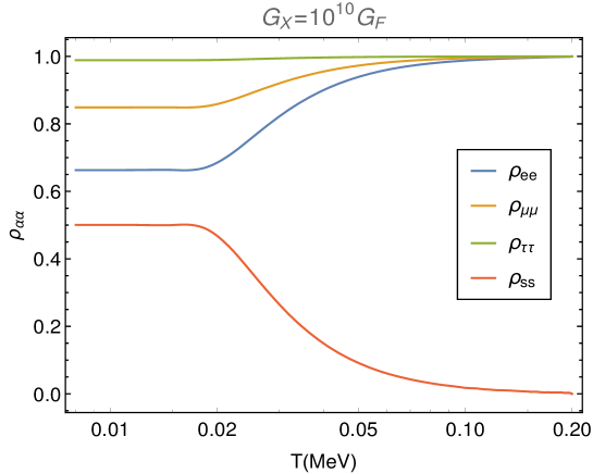
Then we solve the QKEs for the neutrino scenario with self interaction in the sterile neutrino sector. We have plotted number density against temperature in fig. (1). It is clear from the fig. (1) that strong self interaction within sterile neutrinos, , can prevent the mixing between active and sterile neutrinos till sub MeV scales. Moreover, after sterile neutrinos come into equilibrium with active neutrinos, all four neutrinos do not contribute equally to the . They redistribute themselves such that always remains close to 3 because of the self interaction, which is in the allowed range obtained from the BBN and CMB data. Therefore, self interaction successfully evades all cosmological constraints.
3 Perturbation equations
In this section we briefly describe the perturbation theory in the presence of self interacting sterile neutrinos. Perturbation equations for neutrinos are solved in mass eigenstates. Therefore the density matrix in mass eigen basis represents the distribution function for the the neutrinos. So, we write
| (18) |
Naturally this distribution function is not normalized to one. However, for the purpose of calculating perturbed Boltzmann equation, normalization of the distribution function is not necessary. has to be evaluated from the QKE and it depends on time. We perturb this distribution function as,[50]
| (19) |
where is the zeroth order Fermi-Dirac distribution function. Here denotes the spatial coordinates, is the conformal time and is the amplitude of momentum divided by the energy (see ref [50]). are the directions of the momentum vectors. The phase space distribution evolves according to the Boltzmann equation
| (20) |
Since has time dependence, will introduce a time derivative of in the Boltzmann equation. From fig. (1) we see that the changes in occurs at a temperature above MeV. However, the Boltzmann codes like CAMB or CLASS starts solving the perturbation equations from much lower energy scales. Therefore, the remains constant and time derivative does not appear in the Boltzmann hierarchy equation. The term on the right hand side of eq. (20) is the collision term. This term is zero in the standard three neutrino case. In relaxation time approximation for the self interacting neutrinos this term is written as [51]
where
Here, the value of is taken from the solution of QKEs eq. (11). Using this collision term we can rewrite the Boltzmann equation as[50]
| (21) |
where . We expand in a Legendre series as
| (22) |
Using this series expansion we write the Boltzmann equation as a hierarchy of multipoles.
| (23a) | |||
| (23b) | |||
| (23c) | |||
| (23d) | |||
Following ref [37] we have kept the collision term zero in the and equations for conserving particle number and momentum. We have modified the Boltzmann code CLASS [52, 53, 54] with the above mentioned equations. Similarly, as we have introduced scalar perturbations in eq. (19) we can introduce tensor perturbations in the distribution function.
| (24) |
where is a traceless-transverse tensor and is the neutrino tensor transfer function. Using the similar procedure like scalar perturbation we can come up with a similar set of equations for like eq. (23). These equations can be found in ref [55]. We have changed those equations in CLASS and could not find any visible effect on mode spectrum of CMB.
4 Effect on CMB
(a) (b)
We would compare two models here in this paper. The first model is CDM with three massive neutrinos which has masses corresponding to normal hierarchy and lowest neutrino mass to be eV. Such a small mass for the lowest massive neutrino makes it effectively massless. Here all the three neutrinos have degeneracy equal to one. We will call this model CDM only in the rest of the paper. The second model has four massive neutrinos but they have different degeneracy factors and self interaction in sterile sector as described in the earlier sections. Mass of the fourth massive neutrino is considered to be 0.2 eV which is the bestfit value of MiniBoone[4]. We will refer to this model as SI model. Self interacting sterile neutrinos affect CMB in three different ways. First, the mass of the sterile neutrino effects the CMB similarly the way massive neutrinos effect. It shifts the peaks of the CMB towards the lower values of and decreases the height of the peaks too. The second factor which comes into the play is the degeneracy of the mass eigenstates. The degeneracy of these mass eigenstates can be written as
| (25) |
For the parameters defined in the earlier sections and the values of plotted in fig. (1) the degeneracy of the corresponding mass eigenstates are given in table 1.
| Mass () in eV | 0.00001 | 0.009 | 0.05 | 0.2 |
|---|---|---|---|---|
| Degeneracy() | 0.69 | 0.84 | 0.90 | 0.56 |
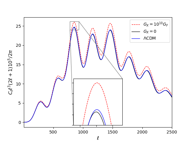
In fig. (2) we have plotted CMB temperature () power spectra for CDM model and then that with the values of neutrino masses and degeneracy factors of table 1. The peaks of CMB shifts towards the lower values of in case. It is shown in the zoomed inset panel of the plot (a) in fig. (2). However, the effect of a 0.2 eV massive neutrino becomes milder due to its degeneracy factor of 0.56. It is because the fraction of neutrino energy density to the critical density of universe () depends on the mass of neutrinos and their degeneracies in the following way, [56]444CAMB and CLASS, both of these boltzman codes take care of the effects of degeneracies of neutrinos in similar way.
| (26) |
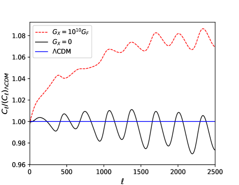
This means that a mass eigen state with degeneracy factor less than one contributes less in as compared to a mass eigen state with same mass but degeneracy facotor one. Therefore, in SI model, contribution of each state in is less as their degeneracy factors are less than one. Hence their effect on CMB power spectrum will be milder as compared to the case where each state has degeneracy factor one. Third effect comes from the self interaction in sterile neutrinos. This effect is also similar to the effect of interactions in active neutrino sector studied in literature [41]. Self-interaction helps to grow the perturbations on small scales and therefore the peaks of the CMB grows up due to that. This effect is visible in both the plots (a) and (b) of fig. (2). In panel (a) where the power spectrum for different cases is plotted, we can see that there is a increase in the height of the peaks for . In panel (b), the ratio of power spectrum for and with CDM was plotted. The effect of of self-interaction is clearly seen to increase the amplitudes of CMB power spectrum for all values of . In these plots the same mass and degeneracy of table 1 was used for for and cases.
| Parameter | CDM | SI model |
|---|---|---|
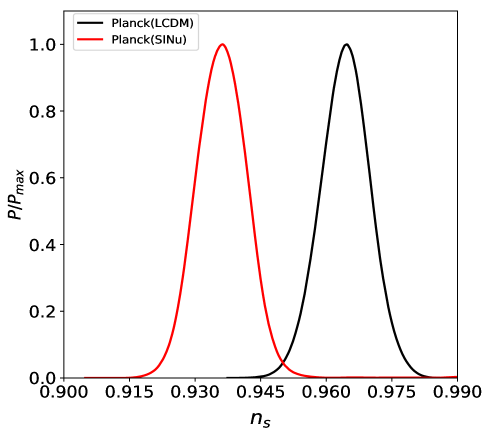
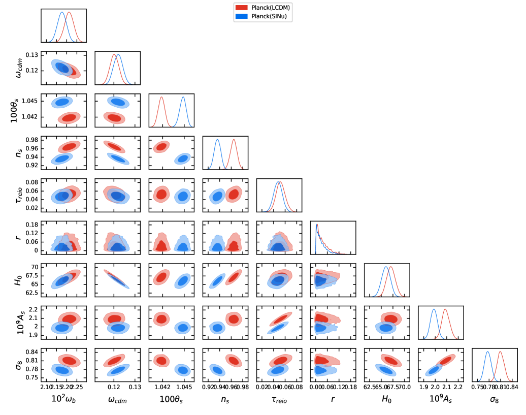
Next, we analyse the effect of self interacting sterile neutrinos on cosmological parameters in the light of Planck observations [22]. We use Planck CMB observations [22] for temperature anisotropy power spectrum over the multipole range - and Planck CMB polarization data for the multipole range - only. For this purpose we have used the Planck high- and low- likelihood as defined in ref. [22, 40]. We will refer these data combined as Planck data. For doing the Markov Chain Monte Carlo (MCMC) analysis of the parameter space we have used Montepython [57]. Sterile neutrino parameters were kept fixed at , and eV and all seven cosmological parameters were allowed to vary. The seven cosmological parameters are as follows: The ratio of density of cold dark matter and baryonic matter evaluated today to the critical density multiplied by squared of the reduced Hubble parameter is and respectively. Acoustic scale of baryon acoustic oscillation is . and are the amplitude and the spectral index of the primordial density perturbations respectively. Optical depth to the epoch of re-ionization is denoted by . And tensor-to-scalar ratio is called . Present Hubble value and the amplitude of matter power spectrum smoothed over 8 scale, known as , are the derived parameters. We list down the best-fit values of these cosmological parameters for the two different models in table 2. More details about the MCMC is given in appendix A We have found that both these models have equivalent statistical significance of fitting Planck CMB data. In fig. (3) the posterior distribution of spectral index has been shown. We see that both the posteriors have same width. Moreover, from table 2 we can find out that the one sigma error for is even smaller for the SI model. However, there is a increase of 1.45 in the maximum value of likelihood) in the case of SI model compared to CDM.
Figures 4 shows the 1- and 2- contours for - planes. The 1- maximum value of drops down from 0.0460 to 0.0383 for introducing self-interaction in sterile neutrino. In last section we have pointed out that self-interaction among sterile neutrinos have negligible effect on modes of CMB. However, there is an indirect effect on spectrum in this scenario. The increase in the amplitude of spectrum in SI model forces other cosmological parameters like and to change. This changes effects the modes in lower values of . To adjust those changes the value of comes down.
5 Inflation models
In this section we will consider four inflation models. More models can be studied in this context. However, we find that for these four models our shifts in cosmological parameters make significant implications. The four models are Starobinsky inflation, natural inflation, quartic hilltop inflation and Coleman-Weinberg inflation. Before going to the details of the models, we briefly review the relations of spectral index and tensor-to-scalar ratio with the inflaton potential. If the potential of inflation field is denoted by then the first order slow roll parameters are written in terms of inflaton potential as
| (27) |
Number of -foldings from the horizon exit of the pivot scale to the end of inflation is
| (28) |
where is the value of the background inflaton field when pivot scale made the horizon exit, and is at the end of inflation. Therefore, is a function of . The value of scalar spectral index is calculated at the and it is
| (29) |
Similarly tensor-to-scalar ratio is given by
| (30) |
Amplitude of density perturbation is
| (31) |
With these tools in hand we can calculate the spectral index and tensor-to-scalar ratio from any given inflation potential.
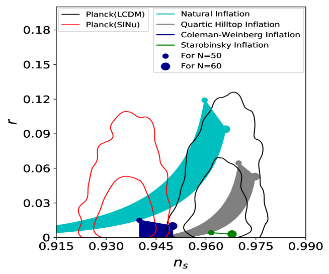
5.1 Starobinsky inflation
The action for the Starobinsky model is written in Jordan frame as
| (32) |
where is a mass scale and is the Ricci scalar. Upon conformal transformation to Einstein frame this action reduces to
| (33) |
where,
| (34) |
and
| (35) |
Inflation ends in this model for . From that value of we follow the procedure described at the beginning of this section and we come up with a value of to be 0.961585 and 0.967833 for 50 and 60 -foldings respectively. is 5.24 and 5.45 respectively. remains negative at these values of and becomes very small, so we get to be 0.004 and 0.003 for and 60. This model of inflation has been the most popular model since the release of Planck 2013 data where tensor-to-scalar ratio was reported to be low enough to accommodate any convex potential. Starobinsky model does not only predict low tensor-to-scalar ratio but also predicts the value of spectral index which fits exactly within 1- level in - plot for CDM cosmology(see fig. (4)). However, the for the case of self-interacting sterile neutrino the prediction of this model lies well outside the 2- range of constrained - values. Since the prediction of this model does not depend on any parameter, this theory cannot be adjusted to fit into the modified of self interacting sterile neutrino. The success of Starobinsky inflation prompted many authors to non-minimally couple a scalar field with the Ricci scalar(). The most popular one is HIggs inflation [58] where the scalar field is considered to be standard model higgs itself. The action in the Jordan frame has the following form
| (36) |
After conformal transformation to the Einstein frame the potential exactly takes the form of eq. (34). Therefore the prediction of this model and Starobinsky model in - plane is absolutely same. So, according to the shifts in in SI case, this model will also be ruled out.
5.2 Natural inflation
Pseudo-Nambu-Goldstone boson were considered to be a suitable candidate to drive inflation unless the advent of Planck data. This model has a free parameter which can be adjusted to shift the values of and . Although the predicted spectral index missed the 1- contour in - plane for CDM cosmology. In our case of self-interacting sterile neutrino the model revives again and the predictions for this model comes well within the 1- contour in -. The potential of the model is given by [59, 60]
| (37) |
determines the scale of the inflation and amplitude of density perturbations. and are independent of but depends on . The predicted region of and falls within the allowed 1- range for self-interacting sterile neutrino and the allowed range for in that case is 3.8 to
5.3 Quartic hilltop inflation
Quartic hilltop represents a set of all models whose potential can be represented as [61]
| (38) |
Naturally the potential written above is incomplete and unbounded from below. Therefore any complete model will consist of other extra terms in potential. For this kind of models, which slowroll parameter among and will violate slowroll condition and thus determine the value of that depends on the other terms of the potential which are not included here. Therefore, value of at the end of inflation varies from model to model. However, for the purpose of a generic discussion we compute the value of with the above mentioned potential only. Similarly like the natural inflation model the amplitude of density perturbation depends on . Spectral index and tensor-to-scalar ratio is just the function of . We vary the value of from 0.01 to 100 to get the values of and shown in fig. (4). For smaller values of , also becomes smaller. For self-interacting sterile neutrino is preferred to be less than 1 and 7 for -foldings 60 and 50 respectively.
5.4 Coleman-Weinberg inflation
Potential of the model is given by [62]
| (39) |
This model of inflation is the Coleman-Weinberg correction to the potential. The model has two parameters and . Although the model works for almost all the values of , since it is the renormalization scale it cannot be above Planck mass. Moreover, the region of horizon exit in the potential corresponds to region for any value of . For and 60 the turns out to be 0.94 and 0.95 respectively. The maximum possible value of for these values of is 0.015 and 0.01. These values of can go down to much smaller values depending on the value of .
6 Discussion and Conclusion
Constraining inflation models on the basis of spectral index and tensor-to-scalar ratio obtained from the CMB data had been the forefront area of research in cosmology and high energy physics for last decades. Inflation models are constrained from CMB observations which place limits on inflation parameters like amplitude of primordial power spectra, tilt of the scalar power spectra and tensor to scalar ratio. In these analyses the base model is normally the CDM cosmology. Although there are many tensions like [63, 64, 65, 66] or tension [67] among different cosmological measurements under CDM framework still it is undeniable that CDM is the best model available so far to fit the CMB data. The need to accommodate sterile neutrinos, motivated by SBL neutrino oscillation experiments, requires one to introduce large self interaction in the sterile neutrino sector. We studied the change in cosmological parameters in this scenario. We find that the best fit values of in CDM model changes to in SI model. This happens because self-interaction in sterile neutrino shifts the CMB peaks in upward. Although there are many theoretical models which, when examined with CMB data, suggests different values of spectral index and tensor-to-scalar ratio, but most of them either use extra cosmological parameters or they decrease the value of likelihood. Interestingly SI model, with the neutrino parameters fixed from MiniBooNE, achieves the similar likelihood values as the CDM model with no other extra free cosmological parameter. The change in inflation parameters make significant impact on the validity of different cosmological models. In this paper we mainly focused on those potentials which have a concave section since self-interacting sterile neutrino did not enhance the tensor-to-scalar ratio. We found that the Starobinsky model which is the best fit model in CDM cosmology is ruled out in the SI cosmology. The similar models which use non-minimal coupling of scalar field to gravity sector for achieving inflation is ruled out too. In addition the quartic hilltop is also disfavored in the SI model which was allowed at 1- level in CDM model. On the other hand some models like natural and Coleman-Weinberg inflation, which were ruled out in the CDM cosmology are now favored. In conclusion if future SBL neutrino oscillation experiments confirms the existence of eV scale sterile neutrino then it will have significant impact on the choice of viable inflation models.
Appendix
Appendix A Details of MCMC
The priors of the seven cosmological parameters are given in table 3. We have used Gaussian prior for our purpose. In case of a maximum and a minimum value was assigned which were 0.5 and 0.0 respectively. Similarly a minimum value of was specified to be .
| Parameter | mean | 1- |
|---|---|---|
| 0.12010 | 0.0013 | |
| 1.04110 | 3e-4 | |
| 3.0447 | 0.015 | |
| 0.9659 | 0.0042 | |
| 0.0543 | 0.008 | |
| 0.06 | 0.04 |
In fig. (5) we can see that two parameters gets affected significantly and these two parameters are spectral index and acoustic scale . Since is the derived parameter from the value of also decreases making the tension even more severe. The amplitude of matter power spectrum smoothed over 8 scale, known as , also reduces because of the effect of massive neutrino on matter power spectrum [68]. We can see from these posterior plots in fig. (5) that the posteriors has almost same for both the models. This makes the two models equivalent in fitting the Planck CMB data.
Acknowledgment
We would like to thank Ningqiang Song for suggestions in solving QKE. We would also like to thank Akhilesh Nautiyal for various helps regarding plotting. We also acknowledge the computation facility, 100TFLOP HPC Cluster, Vikram-100, at Physical Research Laboratory, Ahmedabad, India.
References
- [1] A. Aguilar-Arevalo et al. Evidence for neutrino oscillations from the observation of anti-neutrino(electron) appearance in a anti-neutrino(muon) beam. Phys. Rev., D64:112007, 2001.
- [2] A. A. Aguilar-Arevalo et al. Unexplained Excess of Electron-Like Events From a 1-GeV Neutrino Beam. Phys. Rev. Lett., 102:101802, 2009.
- [3] A. A. Aguilar-Arevalo et al. Event Excess in the MiniBooNE Search for Oscillations. Phys. Rev. Lett., 105:181801, 2010.
- [4] A. A. Aguilar-Arevalo et al. Significant Excess of ElectronLike Events in the MiniBooNE Short-Baseline Neutrino Experiment. Phys. Rev. Lett., 121(22):221801, 2018.
- [5] P. Anselmann et al. First results from the Cr-51 neutrino source experiment with the GALLEX detector. Phys. Lett., B342:440–450, 1995.
- [6] W. Hampel et al. Final results of the Cr-51 neutrino source experiments in GALLEX. Phys. Lett., B420:114–126, 1998.
- [7] G. Mention, M. Fechner, Th. Lasserre, Th. A. Mueller, D. Lhuillier, M. Cribier, and A. Letourneau. The Reactor Antineutrino Anomaly. Phys. Rev., D83:073006, 2011.
- [8] S. Schael et al. Precision electroweak measurements on the resonance. Phys. Rept., 427:257–454, 2006.
- [9] Joachim Kopp, Michele Maltoni, and Thomas Schwetz. Are There Sterile Neutrinos at the eV Scale? Phys. Rev. Lett., 107:091801, 2011.
- [10] Carlo Giunti and Marco Laveder. Status of 3+1 Neutrino Mixing. Phys. Rev., D84:093006, 2011.
- [11] J. M. Conrad, C. M. Ignarra, G. Karagiorgi, M. H. Shaevitz, and J. Spitz. Sterile Neutrino Fits to Short Baseline Neutrino Oscillation Measurements. Adv. High Energy Phys., 2013:163897, 2013.
- [12] Joachim Kopp, Pedro A. N. Machado, Michele Maltoni, and Thomas Schwetz. Sterile Neutrino Oscillations: The Global Picture. JHEP, 05:050, 2013.
- [13] S. Gariazzo, C. Giunti, and M. Laveder. Light Sterile Neutrinos in Cosmology and Short-Baseline Oscillation Experiments. JHEP, 11:211, 2013.
- [14] G. H. Collin, C. A. Argüelles, J. M. Conrad, and M. H. Shaevitz. Sterile Neutrino Fits to Short Baseline Data. Nucl. Phys., B908:354–365, 2016.
- [15] Mona Dentler, Álvaro Hernández-Cabezudo, Joachim Kopp, Pedro A. N. Machado, Michele Maltoni, Ivan Martinez-Soler, and Thomas Schwetz. Updated Global Analysis of Neutrino Oscillations in the Presence of eV-Scale Sterile Neutrinos. JHEP, 08:010, 2018.
- [16] Peter B. Denton, Yasaman Farzan, and Ian M. Shoemaker. Activating the fourth neutrino of the 3+1 scheme. Phys. Rev., D99(3):035003, 2019.
- [17] Bhavesh Chauhan and Subhendra Mohanty. Signature of light sterile neutrinos at IceCube. Phys. Rev., D98(8):083021, 2018.
- [18] Jan Hamann, Steen Hannestad, Georg G. Raffelt, and Yvonne Y. Y. Wong. Sterile neutrinos with eV masses in cosmology: How disfavoured exactly? JCAP, 1109:034, 2011.
- [19] Steen Hannestad, Irene Tamborra, and Thomas Tram. Thermalisation of light sterile neutrinos in the early universe. JCAP, 1207:025, 2012.
- [20] Richard H. Cyburt, Brian D. Fields, Keith A. Olive, and Tsung-Han Yeh. Big Bang Nucleosynthesis: 2015. Rev. Mod. Phys., 88:015004, 2016.
- [21] P. A. R. Ade et al. Planck 2015 results. XIII. Cosmological parameters. Astron. Astrophys., 594:A13, 2016.
- [22] N. Aghanim et al. Planck 2018 results. VI. Cosmological parameters. 2018.
- [23] Steen Hannestad. Neutrino physics from precision cosmology. Prog. Part. Nucl. Phys., 65:185–208, 2010.
- [24] Yvonne Y. Y. Wong. Neutrino mass in cosmology: status and prospects. Ann. Rev. Nucl. Part. Sci., 61:69–98, 2011.
- [25] Julien Lesgourgues and Sergio Pastor. Neutrino mass from Cosmology. Adv. High Energy Phys., 2012:608515, 2012.
- [26] Elena Giusarma, Maria Archidiacono, Roland de Putter, Alessandro Melchiorri, and Olga Mena. Sterile neutrino models and nonminimal cosmologies. Phys. Rev., D85:083522, 2012.
- [27] Chiu Man Ho and Robert J. Scherrer. Sterile Neutrinos and Light Dark Matter Save Each Other. Phys. Rev., D87(6):065016, 2013.
- [28] Graciela Gelmini, Sergio Palomares-Ruiz, and Silvia Pascoli. Low reheating temperature and the visible sterile neutrino. Phys. Rev. Lett., 93:081302, 2004.
- [29] Robert Foot and R. R. Volkas. Reconciling sterile neutrinos with big bang nucleosynthesis. Phys. Rev. Lett., 75:4350, 1995.
- [30] Luis Bento and Zurab Berezhiani. Blocking active sterile neutrino oscillations in the early universe with a Majoron field. Phys. Rev., D64:115015, 2001.
- [31] Steen Hannestad, Rasmus Sloth Hansen, and Thomas Tram. How Self-Interactions can Reconcile Sterile Neutrinos with Cosmology. Phys. Rev. Lett., 112(3):031802, 2014.
- [32] Basudeb Dasgupta and Joachim Kopp. Cosmologically Safe eV-Scale Sterile Neutrinos and Improved Dark Matter Structure. Phys. Rev. Lett., 112(3):031803, 2014.
- [33] Xiaoyong Chu, Basudeb Dasgupta, Mona Dentler, Joachim Kopp, and Ninetta Saviano. Sterile neutrinos with secret interactions - cosmological discord? JCAP, 1811(11):049, 2018.
- [34] Ningqiang Song, M. C. Gonzalez-Garcia, and Jordi Salvado. Cosmological constraints with self-interacting sterile neutrinos. JCAP, 1810(10):055, 2018.
- [35] Alessandro Mirizzi, Gianpiero Mangano, Ofelia Pisanti, and Ninetta Saviano. Collisional production of sterile neutrinos via secret interactions and cosmological implications. Phys. Rev., D91(2):025019, 2015.
- [36] Xiaoyong Chu, Basudeb Dasgupta, and Joachim Kopp. Sterile neutrinos with secret interactions—lasting friendship with cosmology. JCAP, 1510(10):011, 2015.
- [37] Francesco Forastieri, Massimiliano Lattanzi, Gianpiero Mangano, Alessandro Mirizzi, Paolo Natoli, and Ninetta Saviano. Cosmic microwave background constraints on secret interactions among sterile neutrinos. JCAP, 1707(07):038, 2017.
- [38] Ivan Esteban, M. C. Gonzalez-Garcia, Alvaro Hernandez-Cabezudo, Michele Maltoni, and Thomas Schwetz. Global analysis of three-flavour neutrino oscillations: synergies and tensions in the determination of , , and the mass ordering. JHEP, 01:106, 2019.
- [39] P. A. R. Ade et al. Planck 2015 results. XX. Constraints on inflation. Astron. Astrophys., 594:A20, 2016.
- [40] Y. Akrami et al. Planck 2018 results. X. Constraints on inflation. 2018.
- [41] Christina D. Kreisch, Francis-Yan Cyr-Racine, and Olivier Doré. The Neutrino Puzzle: Anomalies, Interactions, and Cosmological Tensions. 2019.
- [42] Gabriela Barenboim, Peter B. Denton, and Isabel M. Oldengott. Constraints on inflation with an extended neutrino sector. Phys. Rev., D99(8):083515, 2019.
- [43] Thomas Tram, Robert Vallance, and Vincent Vennin. Inflation Model Selection meets Dark Radiation. JCAP, 1701(01):046, 2017.
- [44] Y. Fukuda et al. Evidence for oscillation of atmospheric neutrinos. Phys. Rev. Lett., 81:1562–1567, 1998.
- [45] Q. R. Ahmad et al. Measurement of the rate of interactions produced by solar neutrinos at the Sudbury Neutrino Observatory. Phys. Rev. Lett., 87:071301, 2001.
- [46] M. C. Gonzalez-Garcia and Michele Maltoni. Phenomenology with Massive Neutrinos. Phys. Rept., 460:1–129, 2008.
- [47] Maria Archidiacono, Steen Hannestad, Rasmus Sloth Hansen, and Thomas Tram. Cosmology with self-interacting sterile neutrinos and dark matter - A pseudoscalar model. Phys. Rev., D91(6):065021, 2015.
- [48] Alessandro Mirizzi, Ninetta Saviano, Gennaro Miele, and Pasquale Dario Serpico. Light sterile neutrino production in the early universe with dynamical neutrino asymmetries. Phys. Rev., D86:053009, 2012.
- [49] Yi-Zen Chu and Marco Cirelli. Sterile neutrinos, lepton asymmetries, primordial elements: How much of each? Phys. Rev., D74:085015, 2006.
- [50] Chung-Pei Ma and Edmund Bertschinger. Cosmological perturbation theory in the synchronous and conformal Newtonian gauges. Astrophys. J., 455:7–25, 1995.
- [51] Steen Hannestad and Robert J. Scherrer. Selfinteracting warm dark matter. Phys. Rev., D62:043522, 2000.
- [52] Julien Lesgourgues. The Cosmic Linear Anisotropy Solving System (CLASS) I: Overview. 2011.
- [53] Diego Blas, Julien Lesgourgues, and Thomas Tram. The Cosmic Linear Anisotropy Solving System (CLASS) II: Approximation schemes. JCAP, 1107:034, 2011.
- [54] Julien Lesgourgues and Thomas Tram. The Cosmic Linear Anisotropy Solving System (CLASS) IV: efficient implementation of non-cold relics. JCAP, 1109:032, 2011.
- [55] Subhajit Ghosh, Rishi Khatri, and Tuhin S. Roy. Dark neutrino interactions make gravitational waves blue. Phys. Rev., D97(6):063529, 2018.
- [56] Antony Lewis. CAMB Notes (https://cosmologist.info/notes/CAMB.pdf). 2014.
- [57] Benjamin Audren, Julien Lesgourgues, Karim Benabed, and Simon Prunet. Conservative Constraints on Early Cosmology: an illustration of the Monte Python cosmological parameter inference code. JCAP, 1302:001, 2013.
- [58] Fedor L. Bezrukov and Mikhail Shaposhnikov. The Standard Model Higgs boson as the inflaton. Phys. Lett., B659:703–706, 2008.
- [59] Katherine Freese, Joshua A. Frieman, and Angela V. Olinto. Natural inflation with pseudo - Nambu-Goldstone bosons. Phys. Rev. Lett., 65:3233–3236, 1990.
- [60] Katherine Freese and William H. Kinney. On: Natural inflation. Phys. Rev., D70:083512, 2004.
- [61] Kazunori Kohri, Chia-Min Lin, and David H. Lyth. More hilltop inflation models. JCAP, 0712:004, 2007.
- [62] Gabriela Barenboim, Eung Jin Chun, and Hyun Min Lee. Coleman-Weinberg Inflation in light of Planck. Phys. Lett., B730:81–88, 2014.
- [63] Shahab Joudaki et al. KiDS-450: Testing extensions to the standard cosmological model. Mon. Not. Roy. Astron. Soc., 471(2):1259–1279, 2017.
- [64] Sampurn Anand, Prakrut Chaubal, Arindam Mazumdar, and Subhendra Mohanty. Cosmic viscosity as a remedy for tension between PLANCK and LSS data. JCAP, 1711(11):005, 2017.
- [65] Subhendra Mohanty, Sampurn Anand, Prakrut Chaubal, Arindam Mazumdar, and Priyank Parashari. Discrepancy and its solutions. J. Astrophys. Astron., 39(4):46, 2018.
- [66] Gaetano Lambiase, Subhendra Mohanty, Ashish Narang, and Priyank Parashari. Testing dark energy models in the light of tension. Eur. Phys. J., C79(2):141, 2019.
- [67] Jose Luis Bernal, Licia Verde, and Adam G. Riess. The trouble with . JCAP, 1610(10):019, 2016.
- [68] Sampurn Anand, Prakrut Chaubal, Arindam Mazumdar, Subhendra Mohanty, and Priyank Parashari. Bounds on Neutrino Mass in Viscous Cosmology. JCAP, 1805(05):031, 2018.