The REQUIEM Survey I: A Search for Extended Ly–Alpha Nebular Emission Around 31 $z>5.7$ Quasars.

Abstract

The discovery of quasars few hundred megayears after the Big Bang represents a major challenge to our understanding of black holes and galaxy formation and evolution. Their luminosity is produced by extreme gas accretion onto black holes, which already reached masses of $M_{\rm BH}>10^{9}$ M_⊙ by $z\sim 6$. Simultaneously, their host galaxies form hundreds of stars per year, using up gas in the process. To understand which environments are able to sustain the rapid formation of these extreme sources we started a VLT/MUSE effort aimed at characterizing the surroundings of a sample of $5.7<z<6.6$ quasars dubbed: the Reionization Epoch QUasar InvEstigation with MUSE (REQUIEM) survey. We here present results of our searches for extended Ly$\alpha$ halos around the first 31 targets observed as part of this program. Reaching 5–$\sigma$ surface brightness limits of $0.1-1.1\times 10^{-17}$erg s^-1 cm^-2 arcsec^-2 over a 1 arcsec² aperture, we were able to unveil the presence of 12 Ly$\alpha$ nebulae, 8 of which are newly discovered. The detected nebulae show a variety of emission properties and morphologies with luminosities ranging from $8\times 10^{42}$ to $2\times 10^{44}$ erg s^-1, FWHMs between 300 and 1700 km s^-1, sizes $<30$ pkpc, and redshifts consistent with those of the quasar host galaxies. As the first statistical and homogeneous investigation of the circum–galactic medium of massive galaxies at the end of the reionization epoch, the REQUIEM survey enables the study of the evolution of the cool gas surrounding quasars in the first 3 Gyr of the Universe. A comparison with the extended Ly$\alpha$ emission observed around bright (${\rm M}_{\rm 1450}\lesssim-25$ mag) quasars at intermediate redshift indicates little variations on the properties of the cool gas from $z\sim 6$ to $z\sim 3$ followed by a decline in the average surface brightness down to $z\sim 2$.

1 INTRODUCTION

Where do the first quasars form? Two decades after the discovery of the first quasar at $z>6$ (i.e., J1030$+$0524 at $z=6.3$, Fan et al., 2001), this question still puzzles astronomers. Assuming a simple model where a massive black hole grows at the Eddington limit starting at a certain time $t_{0}$ from a seed with mass $M_{\rm BH}(t_{0})=M_{\rm seed}$, the evolution of the mass with time can be expressed as:

$$M_{\rm BH}(t)=M_{\rm seed}\times\exp{\left[f_{\rm Duty}(1-\eta)\frac{t-t_{0}}{t_{\rm Sal}}\right]}$$ (1)

where $f_{\rm Duty}$ is the duty cycle and $\eta$ is the fraction of rest mass energy released during the accretion. The time scale of the mass growth is set by the Salpeter time (Salpeter, 1964): $t_{\rm Sal}=\epsilon\sigma_{\rm T}\,c\,/\,\left(4\pi\,G\,m_{\rm p}\right)=\epsilon\,450\,{\rm Myr}$, where $\sigma_{\rm T}$ is the Thomson cross–section, $m_{\rm p}$ is the proton mass, and $\epsilon$ is the radiation efficiency. In standard radiatively efficient accretion disks, all the energy is radiated away and it is typically assumed that $\epsilon=\eta=0.1$ (Soltan, 1982; Tanaka, & Haiman, 2009; Davis & Laor, 2011; Davies et al., 2019a). Equation 1 implies that, for instance, a $10^{2}$ M_⊙ remnant of a PoP III star at $z=30$ needs to accrete at the Eddington limit for its entire life ($f_{\rm Duty}=1$) to reach a black hole mass $>10^{9}$ M_⊙ at $z\sim 6$, as observed in quasars (e.g., Mortlock et al., 2011; De Rosa et al., 2011, 2014; Wu et al., 2015; Mazzucchelli et al., 2017; Bañados et al., 2018; Shen et al., 2019; Reed et al., 2019; Pons et al., 2019). In addition, investigations at mm and sub–mm wavelengths revealed that also the host–galaxies of these first quasars are vigorously growing mass, with star formation rates ${\rm SFR}\gg 100\,{\rm M}_{\odot}\,{\rm yr}^{-1}$ (e.g., Walter et al., 2009; Wang et al., 2013; Willott et al., 2015, 2017; Decarli et al., 2018; Venemans et al., 2012, 2016, 2018; Kim, & Im, 2019; Shao et al., 2019; Wang et al., 2019b; Yang et al., 2019a).

To comprehend how these first quasars form and grow it is important to understand where they are hosted. Efstathiou, & Rees (1988) first proposed that, in the current $\Lambda$CDM paradigm of galaxy formation (e.g., White, & Rees, 1978), only rare high peaks in the density field contain enough gas to build–up the black hole and star mass (taking into account mass losses due to supernova–driven winds) of high–redshift quasars. This scenario is supported by cosmological hydrodynamic simulations (e.g., Sijacki et al., 2009; Costa et al., 2014) and analytical arguments (e.g., Volonteri, & Rees, 2006) showing that only the small fraction of black holes that, by $z\sim 6$, are hosted by $\gtrsim 10^{12}$ M_⊙ dark matter halos can grow efficiently into a population of quasars with masses and accretion rates matching current observational constraints (but see discussion in Fanidakis et al., 2013). To compensate for the rapid gas consumption, the host–galaxies need a continuous replenishment of fresh fuel provided by filamentary streams of $T=10^{4}-10^{5}$ K pristine gas from the intergalactic medium (IGM) and/or by mergers with gas rich halos (e.g., Kereš et al., 2005, 2009; Yoo & Miralda-Escudé, 2004; Volonteri & Rees, 2005; Volonteri, 2010, 2012; Li et al., 2007; Kereš et al., 2009; Dekel, & Birnboim, 2006; Dekel et al., 2009; Fumagalli et al., 2011; van de Voort et al., 2012; Di Matteo et al., 2012; Habouzit et al., 2019; Mayer, & Bonoli, 2019). Observational validations of this framework can be set by the detection of gas reservoirs and satellites in the so–called circum–galactic medium (CGM, empirically defined as the regions within a few hundreds of kiloparsecs from a galaxy) of high–redshift quasars.

Historically, information on the CGM has been provided by absorption signatures imprinted on background sightlines. This revealed the presence of halos of cool and enriched gas extending to $\sim 200$ pkpc from high–redshift galaxies (e.g., Steidel et al., 1994; Bahcall, & Spitzer, 1969; Chen, & Tinker, 2008; Chen et al., 2010a, b; Gauthier et al., 2010; Nielsen et al., 2013a, b; Churchill et al., 2013a; Werk et al., 2016; Tumlinson et al., 2017). In particular, this technique applied on close projected quasar pairs revealed that intermediate redshift quasars are surrounded by massive ($>10^{10}$ M_⊙), metal rich ($Z\gtrsim 0.1Z_{\odot}$), and cool ($T\sim 10^{4}$ K) gas reservoirs (e.g., Bowen et al., 2006; Hennawi et al., 2006; Hennawi, & Prochaska, 2007; Decarli et al., 2009; Prochaska, & Hennawi, 2009; Prochaska et al., 2013a, b; Farina et al., 2013, 2014; Johnson et al., 2015; Lau et al., 2016, 2018). However, the rapid drop in the number density of bright background sources with redshift, make the absorption studies to lose effectiveness at $z\gtrsim 4$.

A promising way to push investigation of the CGM of quasars up to the epoch of reionization is to probe the cool gas in emission. The strong flux of UV photons radiating from the AGN can be reprocessed in the hydrogen Ly$\alpha$ line at 1215.7 Å (Lyman, 1906; Millikan, 1920) by the surrounding gas, giving rise to an extended “fuzz” of fluorescent Ly$\alpha$ emission (e.g., Rees, 1988; Haiman & Rees, 2001; Alam & Miralda-Escudé, 2002). Several pioneering efforts have been performed to reveal such halos in the vicinity of $z\sim 2-4$ quasars (e.g., Heckman et al., 1991a, b; Christensen et al., 2006; North et al., 2012; Hennawi & Prochaska, 2013; Roche et al., 2014; Herenz et al., 2015; Arrigoni Battaia et al., 2016, 2019a). This led to the general consensus that $10-50$ kpc nebulae are (almost) ubiquitous around intermediate redshift quasars, and that a few objects (typically associated with galaxy overdensities) are surrounded by giant Ly$\alpha$ nebulae with sizes $>300$ kpc, i.e. larger than the expected virial radius for such systems (e.g., Cantalupo et al., 2014; Martin et al., 2014; Hennawi et al., 2015; Cai et al., 2017).

A change of gear in these searches was driven by the recent development of the new generation of sensitive integral field spectrographs (IFS) on 10–m class telescopes, i.e. the Multi–Unit Spectroscopic Explorer (MUSE; Bacon et al., 2010) on the ESO/VLT and the Keck Cosmic Web Imager (KCWI; Morrissey et al., 2012, 2018) on the Keck II telescope. These instruments have been successfully exploited to map the diffuse gas in the CGM of hundreds of intermediate redshift galaxies (e.g., Wisotzki et al., 2016; Leclercq et al., 2017; Erb et al., 2018) and quasars (e.g., Martin et al., 2014; Husband et al., 2015; Borisova et al., 2016; Fumagalli et al., 2016; Arrigoni Battaia et al., 2018a, 2019a, 2019b; Ginolfi et al., 2018; Lusso et al., 2019; Cai et al., 2019). The picture emerging is that the cool gas around $z\sim 2-4$ radio–quiet quasars has a quiescent kinematics and it is likely to be constituted by a population of compact (with sizes of $\lesssim 50$ pc) dense ($n_{\rm H}\gtrsim 1$ cm^-3) clouds that are optically thin to the quasar radiation (e.g., Hennawi & Prochaska, 2013; Hennawi et al., 2015; Arrigoni Battaia et al., 2015b; Cantalupo, 2017; Cantalupo et al., 2019).

However, by $z=4$ the Universe is already 1.5 Gyr old and a population of massive, quiescent galaxies is already in place (e.g., Straatman et al., 2014, 2016). To probe the first stages of galaxy formation it is thus necessary to push these studies to $z\gtrsim 6$. To date, extended Ly$\alpha$ halos have been reported only for a handful of $z\sim 6$ quasars exploiting different techniques: narrow–band imaging (Goto et al., 2009; Decarli et al., 2012; Momose et al., 2019), long–slit spectroscopy (Willott et al., 2011; Goto et al., 2012; Roche et al., 2014), and IFS (Farina et al., 2017; Drake et al., 2019). This small sample showed that the first quasars can be surrounded by extended nebulae with luminosities up to ${\rm L}({\rm Ly}\alpha)\sim 10^{44}$ erg s^-1 and sizes $\lesssim 40$ pkpc. However, a detailed interpretation of these results is hampered by the small number statistic and by the heterogeneity of the data.

To overcome these limitations, we started the Reionization Epoch QUasar InvEstigation with MUSE (REQUIEM) survey aimed at performing a statistical and homogeneous census of the close environment of the first quasars. In this Paper, we report results from the investigation of the first 31 $5.7<z<6.6$ quasars part of this ongoing program (including the re–analysis of MUSE data from Farina et al. 2017 and Drake et al. 2019), focusing our attention on the properties of the extended Ly$\alpha$ halos as tracer of the gas reservoirs able to fuel the activity of the first quasars. We defer the analysis of the close galactic environment of these systems to a future paper.

To summarize, the analysis of the MUSE observations (see section 3) of the 31 targets presented in section 2 with the procedure described in section 4 led to the discovery of 12 extended Ly$\alpha$ nebulae above a surface brightness limit of ${\rm SB}_{\rm Ly\alpha}\sim{\rm few}\times 10^{18}$ erg s^-1 cm^-2 arcsec^-2 ($\sim 40\%$ of the cases, see section 5). In section 5 we report on the attributes of the detected halos, we compare them with the properties of the quasar host galaxies and of the central supermassive black holes, and we test for possible signatures of CGM evolution down to $z\sim 3$. Finally, a summary is given in section 6.

Throughout this paper we assume a concordance cosmology with H₀=70 km s^-1 Mpc^-1, $\Omega_{\rm M}$=0.3, and $\Omega_{\Lambda}$=1-$\Omega_{\rm M}$=0.7. In this cosmology, at $z$=6.2 (the average redshift of our sample) the Universe is 0.877 Gyr old, and an angular scale of $\theta$$=$1″ corresponds a proper transverse separation of 5.6 kpc. We remind the reader that MUSE is able to cover the Ly$\alpha$ line up to redshift $z\sim 6.6$ at a spectral resolution of $R=\lambda/\Delta\lambda\sim 3500$ at $\lambda\sim 9000$ Å with a spatial sampling of $0\farcs 2\times 0\farcs 2$ (corresponding to 1.1 pkpc$\times$1.1 pkpc at $z=6$) over a $\sim 1$ arcmin² field–of–view.

2 SAMPLE SELECTION

Our sample consists of 31 quasars in the redshift range $5.77<z<6.62$ located in the southern sky (e.g., Fan et al., 2001, 2003, 2006; Willott et al., 2007, 2010; Venemans et al., 2013; Jiang et al., 2016; Bañados et al., 2016; Reed et al., 2017; Mazzucchelli et al., 2017; Matsuoka et al., 2018; Wang et al., 2019a; Yang et al., 2019b). This includes all available MUSE observations of $z>5.7$ quasars present in the ESO Archive at the time of writing (Aug. 2019). These quasars have an average redshift of $\langle z\rangle=6.22$ and an average absolute magnitude of $\langle{\rm M}_{\rm 1450}\rangle=-26.9$ mag (see section 2 and Figure 1). Among these, only J2228$+$0110 is a confirmed radio–loud quasar (considering radio–loud quasars as having $R$$=$$f_{\nu,\,5{\rm GHz}}$$/$$f_{\nu,\,4400{\rm Ang.}}$$>$$10$, Kellermann et al., 1989; Bañados et al., 2015b , in prep.).

In the following we will refer to the entire dataset as our full sample, and to the subset of 23 quasars with ${\rm M}_{\rm 1450}<-25.25$ mag and $5.95<z<6.62$ as our core sample. This well defined sub–sample is highly representative of the high–$z$ population of luminous quasars (see Figure 1) and largely overlaps with the survey of dust continuum and [C ii] 158 $\mu$m fine–structure emission lines in $z>6$ quasar host–galaxies using the Atacama Large Millimeter Array (ALMA) presented in Decarli et al. (2017, 2018) and Venemans et al. (2018).

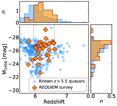
Figure 1: Distribution of all $z>5.5$ quasars known to date in the redshift vs. absolute magnitude plane at 1450 Å  (light blue circles and histograms). Orange diamonds and histograms mark targets from our survey. Histograms are normalized by the total number of targets and by the bin size (with steps $0.15$ in redshift and of $0.6$ mag in absolute magnitude). The limits in luminosity and redshift of our core sample (see section 2) are plotted as gray dashed lines. The five quasars outside these boundaries are: J0129$-$0035 at $z=5.78$, J1044$-$0125 at $z=5.78$, J2228$+$0110 at $z=5.90$, J0055$+$0146 at $z=6.01$, J2216$-$0016 at $z=6.10$, J2219$+$0102 at $z=6.15$, J2229$+$1457 at $z=6.15$, and J2318$-$3113 at $z=6.44$. A 2D Kolmogorov–Smirnov test (Fasano & Franceschini, 1987) performed with bootstrap re–sampling of the parent dataset of the $5.95<z<6.62$ and ${\rm M}_{\rm 1450}<-25.25$ mag quasars does not refute the null hypothesis that our core sample has a different distribution as the parent dataset distribution ($p-{\rm value}\gtrsim 0.2$).

Table 1: Quasars observed with MUSE in decreasing redshift order

ID	RA	Dec.	Redshift	M1450	Prog. ID.	Exp. Time	Image Quality	SB${}_{5\,\sigma}^{1}$
	(J2000)	(J2000)		(mag)		(sec.)	(″)	(erg s-1 cm-2 arcsec-2)
J0305$-$3150	03:05:16.916	$-$31:50:55.90	6.6145$\pm$0.0001	$-$26.12	string094.B-0893	string8640.	0.53	0.29$\times$10-17
P323$+$12	21:32:33.191	$+$12:17:55.26	6.5881$\pm$0.0003	$-$27.06	0101.A-0656	string2964.	0.85	0.48$\times$10-17
P231$-$20	15:26:37.841	$-$20:50:00.66	6.5864$\pm$0.0005string	$-$27.14	string099.A-0682	11856.	0.63	0.30$\times$10-17
P036$+$03	02:26:01.876	$+$03:02:59.39	6.5412$\pm$0.0018	$-$27.28	0101.A-0656	string2964.	0.61	0.33$\times$10-17
J2318$-$3113	23:18:18.351	$-$31:13:46.35	6.4435$\pm$0.0004string	$-$26.06	0101.A-0656	string2964.	0.65	0.54$\times$10-17
P183$+$05	12:12:26.981	$+$05:05:33.49	6.4386$\pm$0.0004string	$-$26.98	string099.A-0682	string2964.	0.62	0.92$\times$10-17
J0210$-$0456	02:10:13.190	$-$04:56:20.90	6.4323$\pm$0.0005	$-$24.47	0103.A-0562	string2964.	1.24	0.26$\times$10-17
J2329$-$0301	23:29:08.275	$-$03:01:58.80	6.4164$\pm$0.0008	$-$25.19	string60.A-9321	string7170.	0.65	0.18$\times$10-17
J1152$+$0055	11:52:21.269	$+$00:55:36.69	6.3643$\pm$0.0005string	$-$25.30	0103.A-0562	string2964.	1.18	0.90$\times$10-17
J2211$-$3206	22:11:12.391	$-$32:06:12.94	6.3394$\pm$0.0010string	$-$26.66	0101.A-0656	string2964.	0.73	1.49$\times$10-17
J0142$-$3327	01:42:43.727	$-$33:27:45.47	6.3379$\pm$0.0004string	$-$27.76	0101.A-0656	string2964.	0.71	1.11$\times$10-17
J0100$+$2802	01:00:13.027	$+$28:02:25.84	6.3258$\pm$0.0010	$-$29.09	0101.A-0656	string2964.	1.29	1.13$\times$10-17
J1030$+$0524	10:30:27.098	$+$05:24:55.00	6.3000$\pm$0.0002	$-$26.93	string095.A-0714	23152.	0.51	0.08$\times$10-17
P308$-$21	20:32:09.996	$-$21:14:02.31	6.2341$\pm$0.0005string	$-$26.29	string099.A-0682	17784.	0.77	0.26$\times$10-17
P065$-$26	04:21:38.052	$-$26:57:15.60	6.1877$\pm$0.0005string	$-$27.21	0101.A-0656	string2964.	0.68	0.25$\times$10-17
P359$-$06	23:56:32.455	$-$06:22:59.26	6.1722$\pm$0.0004string	$-$26.74	0101.A-0656	string2964.	0.58	0.28$\times$10-17
J2229$+$1457	22:29:01.649	$+$14:57:08.99	6.1517$\pm$0.0005	$-$24.72	0103.A-0562	string2964.	0.54	0.27$\times$10-17
P217$-$16	14:28:21.394	$-$16:02:43.29	6.1498$\pm$0.0011string	$-$26.89	0101.A-0656	string2964.	0.90	0.32$\times$10-17
J2219$+$0102	22:19:17.217	$+$01:02:48.90	6.1492$\pm$0.0002	$-$22.54	0103.A-0562	string2964.	0.69	0.48$\times$10-17
J2318$-$3029	23:18:33.100	$-$30:29:33.37	6.1458$\pm$0.0005string	$-$26.16	0101.A-0656	string2964.	0.73	0.30$\times$10-17
J1509$-$1749	15:09:41.778	$-$17:49:26.80	6.1225$\pm$0.0007string	$-$27.09	0101.A-0656	string2964.	0.88	0.46$\times$10-17
J2216$-$0016	22:16:44.473	$-$00:16:50.10	6.0962$\pm$0.0003	$-$23.82	0103.A-0562	string2964.	1.12	0.48$\times$10-17
J2100$-$1715	21:00:54.616	$-$17:15:22.50	6.0812$\pm$0.0005string	$-$25.50	string297.A-5054	13338.	0.67	0.23$\times$10-17
J2054$-$0005	20:54:06.481	$-$00:05:14.80	6.0391$\pm$0.0001	$-$26.15	0101.A-0656	string3869.	0.81	0.24$\times$10-17
P340$-$18	22:40:48.997	$-$18:39:43.81	6.01$\pm$0.05	$-$26.36	0101.A-0656	string2964.	0.55	0.26$\times$10-17
J0055$+$0146	00:55:02.910	$+$01:46:18.30	6.0060$\pm$0.0008	$-$24.76	0103.A-0562	string2964.	0.75	0.27$\times$10-17
P009$-$10	00:38:56.522	$-$10:25:53.90	6.0039$\pm$0.0004string	$-$26.50	0101.A-0656	string2964.	0.67	0.27$\times$10-17
P007$+$04	00:28:06.560	$+$04:57:25.68	6.0008$\pm$0.0004string	$-$26.59	0101.A-0656	string2964.	1.19	0.35$\times$10-17
J2228$+$0110	22:28:43.535	$+$01:10:32.20	5.9030$\pm$0.0002	$-$24.47	string095.B-0419	40950.	0.61	0.11$\times$10-17
J1044$-$0125	10:44:33.042	$-$01:25:02.20	5.7847$\pm$0.0007	$-$27.32	0103.A-0562	string2964.	0.94	0.32$\times$10-17
J0129$-$0035	01:29:58.510	$-$00:35:39.70	5.7787$\pm$0.0001	$-$23.83	0103.A-0562	string2964.	1.19	0.26$\times$10-17

References. — Unless otherwise specified, we report systemic redshifts measured from the [C ii] 158 $\mu$m emission lines by Decarli et al. (2018).

Note. — Seeing and 5–$\sigma$ surface brightness limits have been estimated on pseudo–narrow–band images obtained collapsing 5 wavelength channels (for a total of 6.25 Å) at the expected location of the Ly$\alpha$ emission of the quasars.

2.1 Notes on Individual Objects

J0305$-$3150

Farina et al. (2017) reported the presence of a faint nebular emission extending $\sim 9$ pkpc toward the southwest of the quasar. In addition, the presence of a Ly$\alpha$ emitter (LAE) at a projected separation of 12.5 kpc suggests that J0305$-$3150 is tracing an overdensity of galaxies. This hypothesis is corroborated by recent high–resolution ALMA imaging that revealed the presence of three [C ii] 158 $\mu$m emitters located within $\sim 40$ kpc and $\sim 1000$ ${\rm km}\,{\rm s}^{-1}$ from the quasar (Venemans et al., 2019). These observations also showed the complex morphology of the host–galaxy, possibly due to interactions with nearby galaxies (Venemans et al., 2019). Ota et al. (2018), using deep narrow–band imaging obtained with the Subaru Telescope Suprime–Cam, reported an LAE number density comparable with the background. However, the displacement between the location of the redshifted Ly$\alpha$ emission and wavelengths with high response of the NB921 filter used (see Fig. 2 in Ota et al., 2018) may have hindered the detection of galaxies associated with the quasar.

P231$-$20

ALMA observations of this quasar revealed the presence of a massive [C ii] 158 $\mu$m bright galaxy in its immediate vicinity (with a projected separation of 13.8 kpc and a velocity difference of 591 ${\rm km}\,{\rm s}^{-1}$, Decarli et al., 2017). A sensitive search for the rest–frame UV emission from this companion galaxy is presented in Mazzucchelli et al. (2019). An additional weaker [C ii] 158 $\mu$m emitter has been identified by Neeleman et al. (2019) 14 kpc south–southeast of the quasar. Deep MUSE observations already revealed the presence of a $\sim 18$ pkpc Ly$\alpha$ nebular emission around this quasar (Drake et al., 2019).

P183$+$05

For this quasar Bañados et al. (2019) reported the presence of a proximate damped Ly$\alpha$ absorption system (pDLA) located at $z$=6.40392 (1400 km s^-1 away from the quasar host galaxy), making this system the highest redshift pDLA known to date. It shows an H i column density of N_HI=10^20.77±0.25 cm^-2 and relative chemical abundances typical of an high redshift low–mass galaxy. The pDLA can act as a coronagraphs and, by blocking its light, it allows one to perform sensitive searches for extended emission associated to the background quasar (e.g., Hennawi et al., 2009). The galaxy originating the pDLA is not detected as a Ly$\alpha$ line down–the–barrel in the MUSE quasar’s spectrum (see Figure 15 in Appendix A). However, it could be located at a larger impact parameter (e.g., Neeleman et al., 2016, 2017, 2018; D’Odorico et al., 2018). The possibility to detected the galaxy in the full MUSE datacube, both in emission and as a shadow against the extended background Ly$\alpha$ halo, will be explored in a future paper of this series (Farina et al., in prep.).

J2329$-$0301

The Ly$\alpha$ halo of this quasar has been the subject of several studies (Goto et al., 2009, 2012; Willott et al., 2011; Momose et al., 2019; Drake et al., 2019). Goto et al. (2017) reported the complete absence of LAEs down to a narrow–band magnitude of NB906=25.4 mag (at 50% completeness) in the entire field–of–view of the Subaru Telescope Suprime–Cam ($\sim$200 cMpc²).

J0100$+$2802

With ${\rm M}_{\rm 1450}=-29.09$ mag, J0100$+$2802 is the brightest (unlensed) quasar known at $z>6$ (Wu et al., 2015). Sub–arcsecond resolution observations of the [C ii] 158 $\mu$m and CO emission lines suggest that the host galaxy has a dynamical mass of only $\sim 1.9\times 10^{11}$ M_⊙ (Wang et al., 2019b). Given this high luminosity, its proximity zone appears to be small [$R_{\rm p}=(7.12\pm 0.13)$ pMpc], implying that this quasar is relatively young, with a quasar age of $t_{\rm QSO}\sim 10^{5}$ years (Eilers et al., 2017; Davies et al., 2019b).

J1030$+$0524

Deep broad band optical and near–IR investigation evidenced an overdensity of Lyman–Break galaxies in the field of this quasar (Morselli et al., 2014; Balmaverde et al., 2017; Decarli et al., 2019a). Searches for the presence of Ly$\alpha$ extended emission around this target has already been investigated with sensitive HST observations by Decarli et al. (2012) and with MUSE by Drake et al. (2019).

P308$-$21

The [C ii] 158 $\mu$m emission line of this quasar host–galaxy is displaced by $\sim$25 kpc and shows an enormous velocity gradient extending across more than 1000 ${\rm km}\,{\rm s}^{-1}$ (Decarli et al., 2017). High–resolution ALMA and HST observations revealed that the host–galaxy emission is split into (at least) three distinct components. The observed gas morphology and kinematics is consistent with the close interaction of a single satellite with the quasar (Decarli et al., 2019b). Deep Chandra observations the companion galaxy might contain a heavily–obscured AGN (Connor et al., 2019). A direct comparison of our new MUSE data with the ALMA [C ii] 158 $\mu$m and dust maps will be presented in a forthcoming paper (Farina et al. in prep.).

J2229$+$1457

With a size of only $R_{\rm p}=(0.45\pm 0.14)$ pMpc, the proximity zone of this object is the smallest among the 31 $5.8\lesssim z\lesssim 6.5$ quasars investigated by Eilers et al. (2017). This suggests a short quasar age ($t_{\rm QSO}\lesssim 10^{5}$ years) for this object (Eilers et al., 2017; Davies et al., 2019b).

J2219$+$0102

This is the faintest target in our survey. Despite the low luminosity of the accretion disk, the host galaxy is undergoing a powerful starburst detected at mm–wavelengths (with an inferred star–formation rate of ${\rm SFR}\sim 250$ M_⊙ yr^-1) and appears to be resolved with a size of 2–3 kpc (Willott et al., 2017).

J2216$-$0016

The rest–frame UV spectrum of this faint quasar shows a N v broad absorption line (Matsuoka et al., 2016). The structure of the [C ii] 158 $\mu$m line appears to be complex, suggesting the presence of a companion galaxy merging with the quasar host–galaxy (Izumi et al., 2018)

J2100$-$1715

Decarli et al. (2017) reported the presence of a [C ii] 158 $\mu$m bright companion located at a projected separation of 60.7 kpc and with a velocity difference of $-$41 ${\rm km}\,{\rm s}^{-1}$ from the quasar’s host galaxy. The search for the Ly$\alpha$ emission arising from this companion in the MUSE data is presented in Mazzucchelli et al. (2019). Drake et al. (2019) reported the absence of extended Ly$\alpha$ emission around this quasar.

P007$+$04

The broad Ly$\alpha$ line of this quasar is truncated by the presence of a pDLA (see Figure 15 in Appendix A). The analysis of the absorbing gas generating this feature and the search for its rest–frame UV counterpart will be presented in a future paper of this series (Farina et al., in prep.).

J2228$+$0110

A faint, extended Ly$\alpha$ emission has been detected by Roche et al. (2014) in deep long–slit spectroscopic observations of this faint radio–loud quasar (with radio–loudness: $R$$\sim$$60$, Bañados et al., 2015b). The presence of the halo was confirmed by Drake et al. (2019) with MUSE observations.

J1044$-$0125

ALMA 0$\farcs$2 resolution observations of the [C ii] 158 $\mu$m fine structure line showed evidence of turbulent gas kinematics in the host galaxy and revealed the possible presence of a faint companion galaxy located at a separation of 4.9 kpc (Wang et al., 2019).

3 OBSERVATIONS AND DATA REDUCTION

Observations of the quasars in our sample have been collected with the MUSE instrument on the VLT telescope YEPUN as a part of the ESO programs: 60.A-9321(A, Science Verification), 094.B-0893(A, PI: Venemans), 095.B-0419(A, PI: Roche), 095.A-0714(A, PI: Karman), 099.A-0682(A, PI: Farina), 0101.A-0656(A, PI: Farina), 0103.A-0562(A, PI: Farina), and 297.A-5054(A, PI: Decarli). Typically, the total time on target was $\sim$50 min, divided into two exposures of 1482 s differentiated by a $<$5^′′ shift and a 90 degree rotation. For eight targets, longer integrations have been acquired (ranging from 65 to 680 min) and the shift and rotation pattern was repeated several times (see section 2)

Data reduction was performed as in Farina et al. (2017) using the MUSE Data Reduction Software version 2.6 (Weilbacher et al., 2012, 2014) complemented by our own set of custom built routines. Basic steps are summarized in the following. Individual exposures were bias subtracted, corrected for flat field and illumination, and calibrated in wavelength and flux. We then subtracted the sky emission and re–sampled the data onto a $0\farcs 2$$\times$$0\farcs$$2$$\times$1.25 Å grid. White light images were then created and used to estimate the relative offsets between different exposures of a single target. From these images we also determined the relative flux scaling between exposures by performing force photometry on sources in the field. Finally, we average–combined the exposures into a single cube. Residual illumination patterns were removed using the Zurich Atmosphere Purge (ZAP) software (version 2.0 Soto et al., 2016), setting the number of eigenspectra (nevals) to 3 and masking sources detected in the white light images. This procedure, however, comes with the price of possibly removing some astronomical flux from the cubes. In the following, we will present results from the “cleaned” datacubes. However, we also double checked for extended emission in the data prior to the use of ZAP. To take voxel–to–voxel correlations into account, that can result in an underestimation of the noise calculated by the pipeline, we rescaled the variance datacube to match the measured variance of the background (see e.g., Bacon et al., 2015; Borisova et al., 2016; Farina et al., 2017; Arrigoni Battaia et al., 2019a). The astrometry solution was refined by matching sources with the Pan–STARRS1 (PS1) data archive (Chambers et al., 2016; Flewelling et al., 2016) or with other available surveys if the field was not covered by the PS1 footprint. We corrected for reddening towards the quasar location using $E(B-V)$ values from Schlafly & Finkbeiner (2011) and assuming R_V=3.1 (e.g., Cardelli et al., 1989; Fitzpatrick, 1999). Absolute flux calibration was obtained matching the $z$–band photometry of sources in the field with PS1 and/or with the Dark Energy Camera Legacy Survey. In section 2 we report the 5–$\sigma$ surface brightness limits estimated over a 1 arcsec² aperture after collapsing 5 wavelength slices that were centered at the expected position of the Ly$\alpha$ line shifted to the systemic redshift of the quasar (SB${}_{5\,\sigma,{\rm Ly\alpha}}^{1}$). These range from SB${}_{5\,\sigma,{\rm Ly\alpha}}^{1}$=0.1 to 1.1$\times$10^-17erg s^-1 cm^-2 arcsec^-2 depending on exposure times, sky conditions, and on the redshift of the quasar. Postage stamps of the quasar vicinities and quasar spectra are shown in Appendix A.

4 SEARCHING FOR EXTENDED EMISSION

An accurate PSF subtraction is necessary to recover the faint signal of the diffuse Ly$\alpha$ emission emerging from the PSF wings of the bright unresolved nuclear component. The steps we executed on each datacube to accomplish this goal are summarized in the following:

1. We removed possible foreground objects located in close proximity to the quasar. To perform this step, we first collapsed the datacube along wavelengths blueward of the redshifted Ly$\alpha$ line location. Due to the Gunn–Peterson effect, the resulting image is virtually free of any object with a redshift consistent with or larger than the quasar’s one. For each source detected in this image we extracted the emission over an aperture 3 times larger than the effective radius. We used this as an empirical model of the object’s light profile. This model was then propagated through the datacube by rescaling it to the flux of source measured at each wavelength channel. Finally, all these models were combined together and subtracted from the datacube.

2. An empirical model of the PSF was directly created from the quasar light by summing up spectral regions virtually free of any extended emission, i.e. $>2500\,{\rm km}\,{\rm s}^{-1}$ from the wavelength of the Ly$\alpha$ line redshifted to the quasar’s systemic redshift. For this procedure, we excluded all channels where the background noise was increased by the presence of bright sky emission lines.

3. In each wavelength layer, the PSF model was rescaled to match the quasar flux measured within a radius of 2 spatial pixels, assuming that the unresolved emission of the AGN dominates within this region.

4. Following a similar procedure as in, e.g., Hennawi & Prochaska (2013); Arrigoni Battaia et al. (2015a); Farina et al. (2017) we created a smoothed $\upchi_{x,y,\lambda}$ cube defined as:

   $${\rm SMOOTH}\left[\upchi_{x,y,\lambda}\right]=$$ (2)

   $$=\frac{{\rm CONVOL}\left[{\rm DATA_{x,y,\lambda}}-{\rm MODEL_{x,y,\lambda}}\right]}{\sqrt{{\rm CONVOL}^{2}\left[\sigma^{2}_{x,y,\lambda}\right]}}$$

   where ${\rm DATA_{x,y,\lambda}}$ is the datacube, ${\rm MODEL_{x,y,\lambda}}$ is the PSF model created in the step above, and $\sigma_{x,y,\lambda}$ is the square root of the variance datacube. The operation ${\rm CONVOL}$ is a convolution with a 3D Gaussian kernel with $\sigma_{\rm spat}$=0$\farcs$2 in each spatial direction and $\sigma_{\rm spec}$=2.50 Å in the spectral direction, and ${\rm CONVOL}^{2}$ denotes a convolution with the square of the smoothing kernel used in ${\rm CONVOL}$.

5. To identify significant extended emission, we then ran a friends–of–friends algorithm that connects voxels that have $S/N$$>$2 in the ${\rm SMOOTH}\left[\upchi_{x,y,\lambda}\right]$ cube. We chose a linking length of 2 voxels (in both spatial and spectral directions). Voxels located within the effective radius of a removed foreground source were excluded. Additionally, voxels contaminated by instrumental artifacts were also excluded. We consider a group identified by the FoF as a halo associated with the quasar if, at the same time: (i) there is at least one voxel with $S/N>2$ within a radius of 1 arcsec in the spatial direction and within $\pm 250$ km s^-1 in the spectral direction from the expected location of the Ly$\alpha$ emission of the quasar; (ii) it contains more than 300 connected voxels (this was empirically derived to avoid contaminations from cosmic rays and/or instrument artifacts not fully removed by the pipeline); and (iii) it spans more than two consecutive channels in the spectral direction.

6. If a halo is detected, we created a 3–dimensional mask containing all connected voxels (${\rm MASK_{x,y,\lambda}}$) and used it to extract information from the ${\rm DATA_{x,y,\lambda}}$$-$${\rm MODEL_{x,y,\lambda}}$ cube.

In Figure 2 we show the results of this procedure applied to the REQUIEM survey dataset. For each object we plot a 11″$\times$11″ (roughly 60 pkpc$\times$60 pkpc at $z=6$) pseudo–narrow–band image centered at the quasar location. The spectral region of the cube defining each narrow–band image was set by the minimum ($\lambda_{\rm min}^{\rm mask}$) and maximum ($\lambda_{\rm Max}^{\rm mask}$) wavelengths covered by ${\rm MASK_{x,y,\lambda}}$ (see Table 2). The black contours highlight regions where significant (as described above) extended emission was detected.

In summary, we report the presence of 12 Ly$\alpha$ nebulae around $z>5.7$ quasars, 8 of which are newly discovered. In the following, we describe the procedure used to extract physical information about each detected nebula.

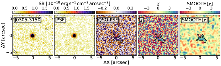
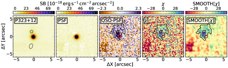
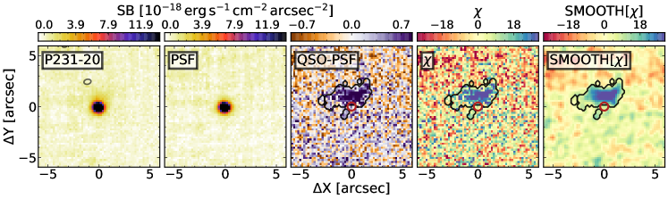
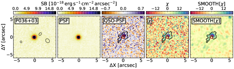
Figure 2: Results from the PSF–subtraction procedure described in section 4. The different panels show the pseudo–narrow–band images obtained by collapsing (from left to right) the ${\rm DATA_{x,y,\lambda}}$, ${\rm MODEL_{x,y,\lambda}}$, ${\rm DATA_{x,y,\lambda}}-{\rm MODEL_{x,y,\lambda}}$, $\upchi_{x,y,\lambda}$, and ${\rm SMOOTH}\left[\upchi_{x,y,\lambda}\right]$ cubes in the wavelength range where extended emission was detected. If no significant nebular emission is present, the collapsed region is between $-$500 and $+$500 ${\rm km}\,{\rm s}^{-1}$. Black contours are constructed by collapsing ${\rm MASK_{x,y,\lambda}}$ along the velocity axis. These are the regions used to extract the spectra of the halos in subsection 4.1. In the left–most panel, the location of the detected (and removed) foreground sources are marked as gray ellipses. Note that saturation spikes from nearby bright stars (e.g. in the bottom left corner of the quasar P323$+$12, or on the top of J1509$-$1749) and/or instrumental artifacts such as IFU–to–IFU edge effects (e.g. for the quasars P183$+$05 and P217$-$16) have been masked during the halo identification procedure but are still shown here.

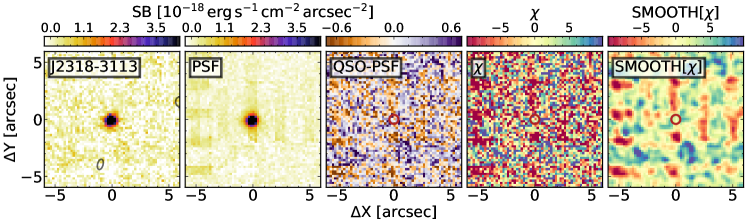
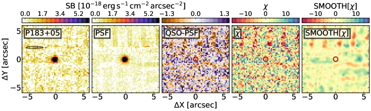
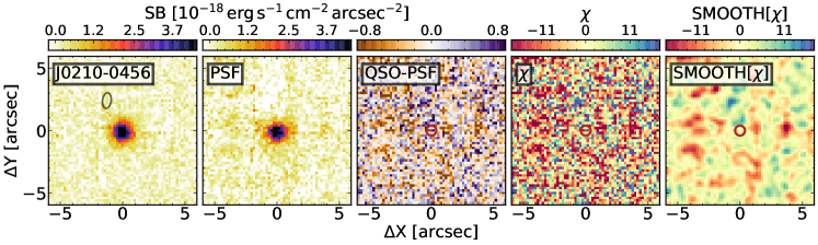
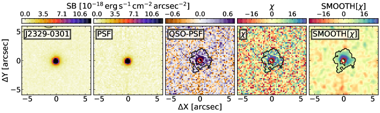
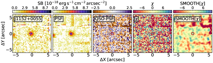
Figure 2: continued.

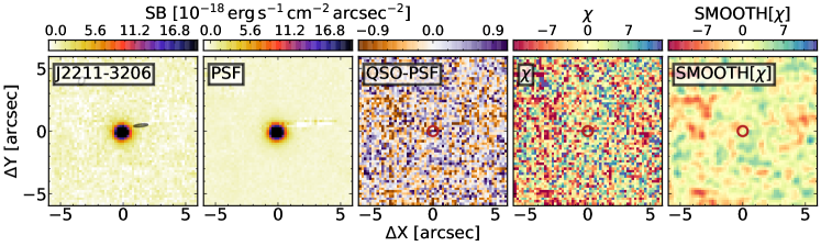
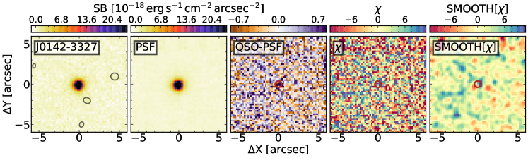
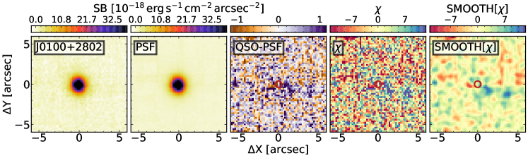
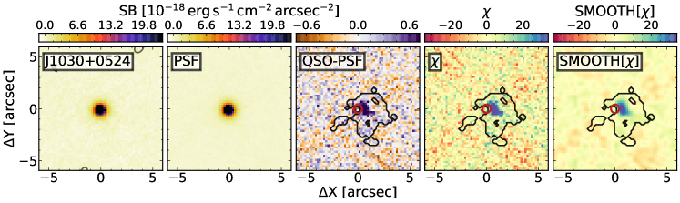
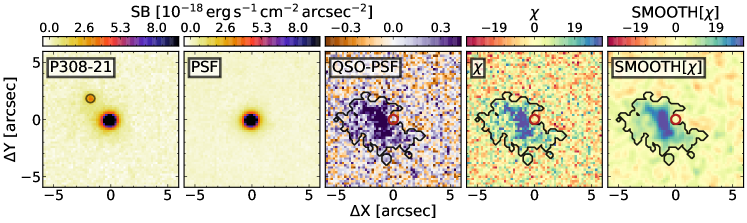
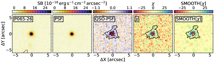
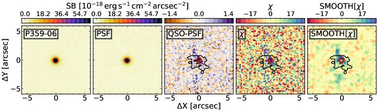
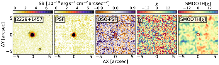
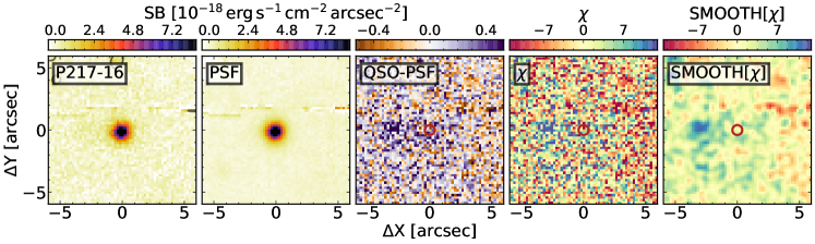
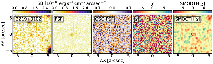
Figure 2: continued.

Figure 2: continued.

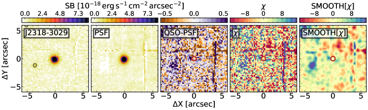
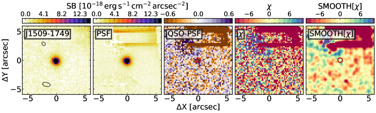
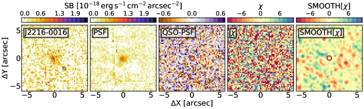
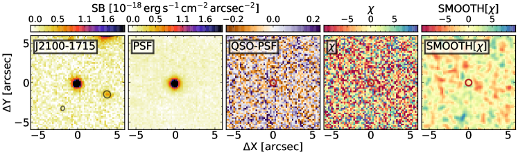
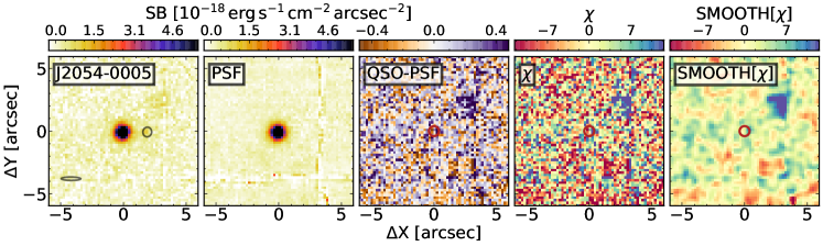
Figure 2: continued.

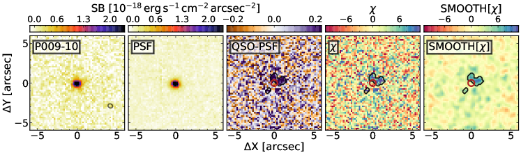
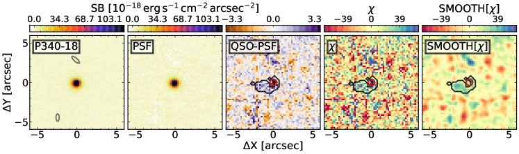
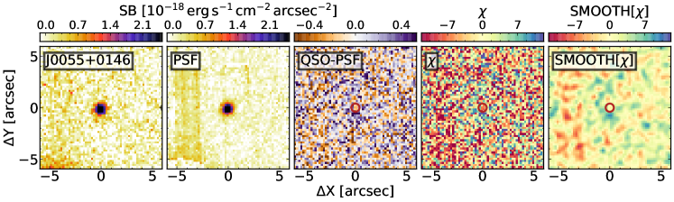
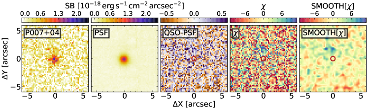
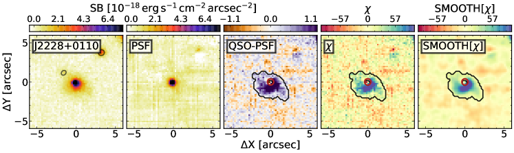
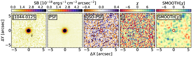
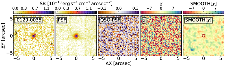
Figure 2: continued.

Figure 2: continued.

4.1 Spectra of the Extended Emission

We extract the nebular emission spectrum using a 2D mask obtained by collapsing ${\rm MASK_{x,y,\lambda}}$ along the spectral axis. The construction of a halo mask described in the previous section is instrumental in obtaining the highest signal–to–noise spectrum of a detected halo. However, given that this procedure is based on a fix cut in signal–to–noise per voxel, it inevitably results in a loss of information at larger radii. For each halo we thus also extract a spectrum from the circular aperture with radius equal to the distance between the quasar and the most distant significant voxel detected in the collapsed ${\rm MASK_{x,y,\lambda}}$ ($d_{\rm QSO}^{\rm mask}$, see Table 2). Spectra extracted over the collapsed mask and over the circular aperture (plotted in red and in yellow in Figure 3) have similar shapes, but the latter shows a systematically higher flux density at each wavelength.

We estimate the central wavelength ($\lambda_{\rm c}$) as a non–parametric flux–and–error–weighted mean of the emission between $\lambda_{\rm min}^{\rm mask}$ and $\lambda_{\rm Max}^{\rm mask}$ (see Table 2 and Figure 3), i.e. without assuming any particular shape for the Ly$\alpha$ line. While in Table 3 we only report measurements from the masked spectrum, we point out that the central wavelengths measured from the 2D masks and from the circular aperture extraction are consistent within the errors, with an average difference of only ($-15\pm 37$) km s^-1. In order to reduce the effects of noise spikes, the FWHMs of the nebular emission were estimated after smoothing spectra extracted from the 2D masks with a Gaussian kernel of $\sigma=2.5$ Å. The derived FHWMs are shown as gray horizontal bars in Figure 3 and listed in Table 3. Finally, total fluxes were calculated by integrating the spectra extracted over the circular apertures between $\lambda_{\rm min}^{\rm mask}$ and $\lambda_{\rm Max}^{\rm mask}$. If a nebula was not detected, we extracted the spectrum over a circular aperture with a fixed radius of 20 pkpc (corresponding to 3$\farcs$5 at $z=6$). From this, we derived the 1–$\sigma$ detection limit as $\sigma^{2}_{\rm Lim}=\sum^{+500\,{\rm km}\,{\rm s}^{-1}}_{-500\,{\rm km}\,{\rm s}^{-1}}\sigma_{\lambda}^{2}/N_{\lambda}$, where $\sigma^{2}_{\lambda}$ is the variance at each wavelength and $N_{\lambda}$ is the number of spectral pixels in the $\pm 500$ km s^-1 stretch from the quasar’s systemic redshift.

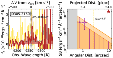
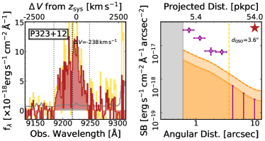
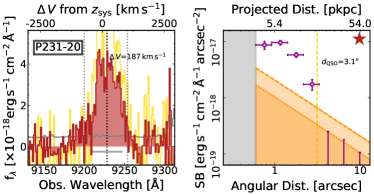
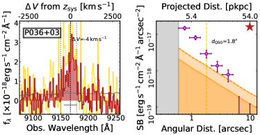
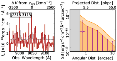
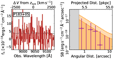
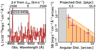
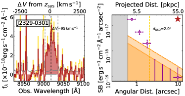
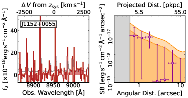
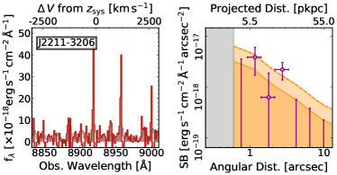
Figure 3: Atlas of spectra and surface brightness profiles of extended emission detected in the REQUIEM survey. Left–hand panel — Spectrum of the nebular emission extracted over the collapsed halo mask as described in subsection 4.1 (red shaded histogram) with corresponding 1–$\sigma$ error (gray histogram). The spectrum extracted over a circular aperture of radius $d_{\rm QSO}$ is also shown as a yellow histogram. The vertical dotted lines mark the wavelength range where the extended emission was detected and the location of its flux–weighted centroid. In the cases where no halo was detected, the spectrum extracted from a circular aperture of radius 20 pkpc is plotted. Right–hand panel — Surface brightness profile extracted over circular annuli evenly spaced in logarithmic space (purple points). The formal 1– and 2–$\sigma$ error in surface brightness are plotted as orange shaded regions (see subsection 4.2 for further details). Stars on the top right corners indicate objects for which significant extended emission has been detected.

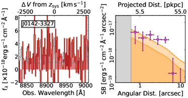
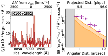
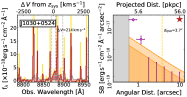
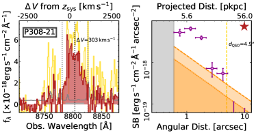
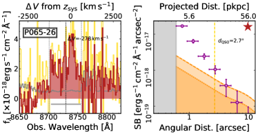
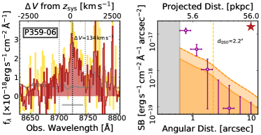
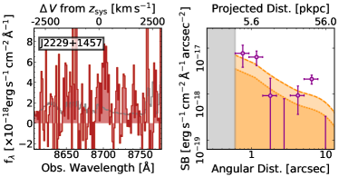
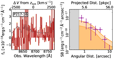
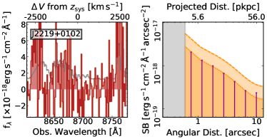
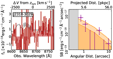
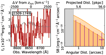
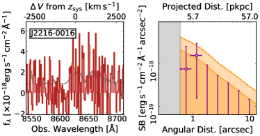
Figure 3: continued.

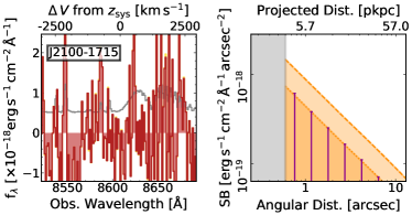
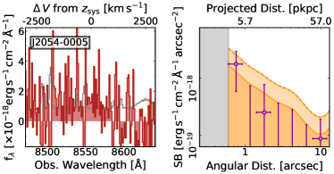
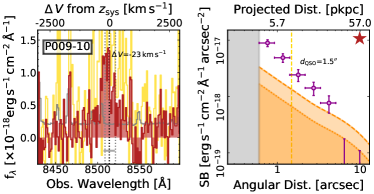
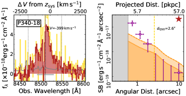
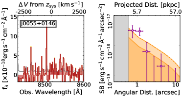
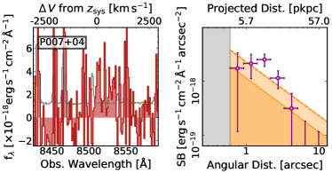
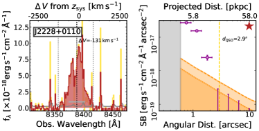
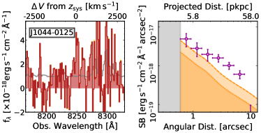
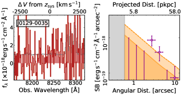
Figure 3: continued.

4.2 Surface Brightness Profiles

The right–hand panels of Figure 3 show circularly averaged surface brightness profiles of the extended emission around each quasar. These are extracted from pseudo–narrow band images constructed summing up spectral channels located between $-500$ and $+500$ km s^-1 of the quasar’s systemic redshift. The choice of a fixed width for the entire sample facilitates a uniform comparison of both detections and non–detections of nebular emission. In addition, this velocity range corresponds to 30 Å, roughly matching the width of the pseudo–narrow–band images used to extract surface brightness profiles by Arrigoni Battaia et al. (2019a) and by Cai et al. (2019) for their samples of $z\sim 2-3$ quasars. However, the size of the bin selected by Arrigoni Battaia et al. and by Cai et al. is twice as large as ours in velocity space. This is also much narrower than previous narrow–band studies targeting high–redshift quasars: e.g., $\sim 100$ Å in Decarli et al. (2012) or $\sim 160$ Å in Momose et al. (2019). While this choice may lead to the loss of some signal from the wings of the nebulae, it allows us to optimize the signal–to–noise ratio of the extended emission whilst being sensitive to faint emission that may be present at larger scales. Before extracting the profile binned in annuli with radii evenly spaced in logarithmic space, we masked regions where apparent instrumental artifacts were present and regions located within the effective radius of the removed foreground sources. Errors associated to each bin of the surface brightness profile were estimated from the collapsed variance datacube.

In addition, from the pseudo–narrow–band images we also derive a noise independent measurement of the size of the nebulae ($d_{\rm QSO}^{\rm fix}$, see Table 2). This is the distance from a quasar where the circularly averaged surface brightness profile drops below a surface–brightness of $(1+z)^{4}\times 3\times 10^{-18}{\rm erg\,s^{-1}\,cm^{-2}\,arcsec^{-2}}$. This value has been chosen to have $d_{\rm QSO}^{\rm fix}\approx d_{\rm QSO}^{\rm mask}$ for data collected with the shortest exposure times.

4.3 Moment Maps

In order to trace the kinematics of the detected extended emission we produced the zeroth, first, and second moment maps of the flux distribution in velocity space (see Figure 4). These maps encode information about the variation of the line centroid velocity and width at different spatial locations. To create the maps, we first smoothed each wavelength layer with a 2D Gaussian kernel with $\sigma=1$ spatial pixel. Then we extracted the the different moments within the ${\rm MASK_{x,y,\lambda}}$ region (i.e. only voxels significantly associated with the halo are included in the maps). Given the complex kinematics of the Ly$\alpha$ emission observed around high redshift quasars (e.g. Martin et al., 2015; Borisova et al., 2016; Ginolfi et al., 2018; Arrigoni Battaia et al., 2018a, 2019a; Drake et al., 2019) and the relatively low spectral resolution of MUSE, the moments are estimated in a non–parametric way by flux–weighting each voxel. In other words, no assumption was made about the 3D shape of the line emitting region.

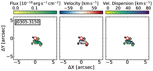
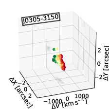
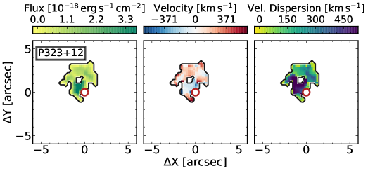
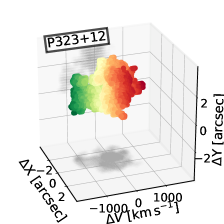
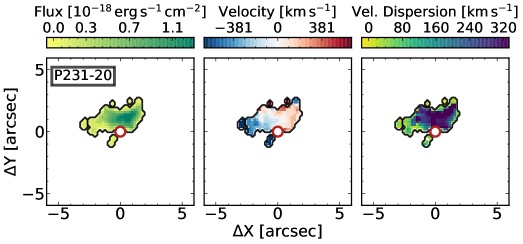
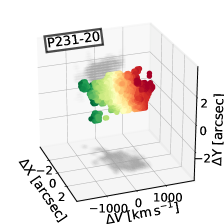
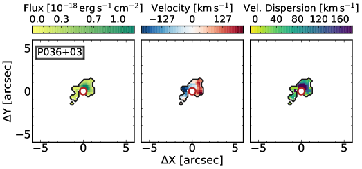
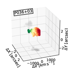
Figure 4: Spatially resolved kinematics of the halos detected in our sample. From left to right: integrated flux (zeroth–moment), velocity–field with respect to the flux–weighted centroid of the line emission (first–moment), and velocity dispersion (second–moment). These maps were obtained as described in subsection 4.3. Note that the maps are not corrected for the finite spectral resolution of MUSE. In the wavelength range explored by our sample, this washes away any information with $\sigma\lesssim 35$ km s^-1. The right–most column shows the 3D visualization of each nebula. Here $\Delta X$ goes from East to West, $\Delta Y$ from South to North, and $\Delta V$ from green to red with respect to the centroid of the extended emission.

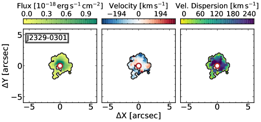
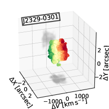
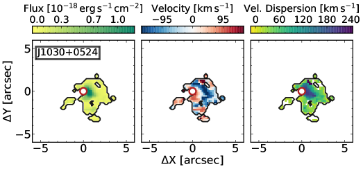
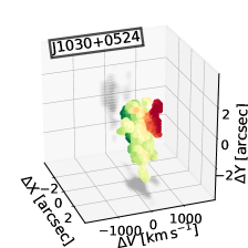
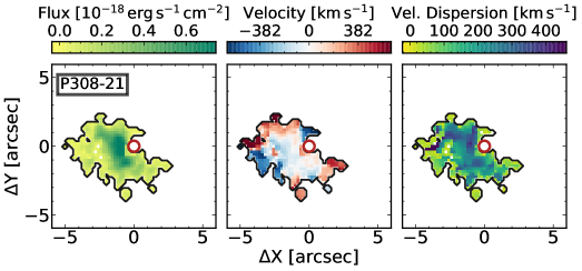
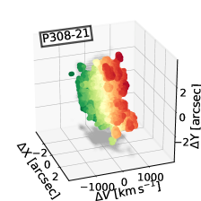
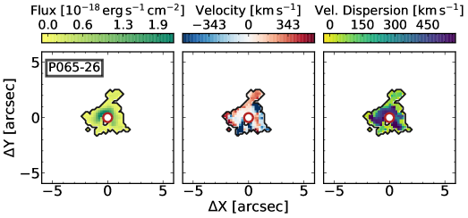
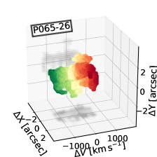
Figure 4: continued.

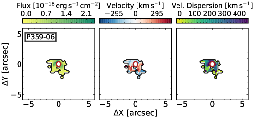
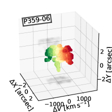
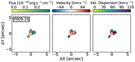
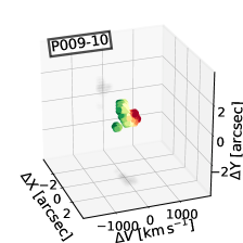
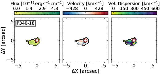
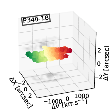
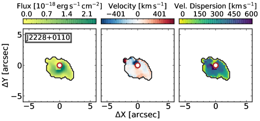
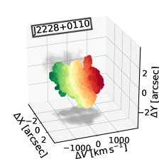
Figure 4: continued.

Table 2: Summary of ${\rm MASK_{x,y,\lambda}}$ properties of identified nebulae.

ID	$\lambda_{\rm min}^{\rm mask}$–$\lambda_{\rm max}^{\rm mask}$	$d_{\rm Max}^{\rm mask}$	$d_{\rm QSO}^{\rm mask}$	$A_{\rm Halo}^{\rm mask}$	$d_{\rm QSO}^{\rm fix}$
	(Å)	(″/pkpc)	(″/pkpc)	(arcsec2)	(″/pkpc)
J0305$-$3150	9255.0–9265.0	3.1$/$16.8	2.5$/$13.5	string1.8	1.3$/$string7.2
P323$+$12	9182.5–9248.8	4.6$/$24.7	3.7$/$20.2	string8.6	3.6$/$19.7
P231$-$20	9200.0–9253.8	5.1$/$27.6	3.1$/$16.8	string7.8	2.8$/$15.3
P036$+$03	9150.0–9178.8	3.6$/$19.4	1.8$/$string9.9	string2.8	1.5$/$string8.1
J2318$-$3113	$\cdots$	$\cdots$	$\cdots$	$\cdots$	$\cdots$
P183$+$05	$\cdots$	$\cdots$	$\cdots$	$\cdots$	$\cdots$
J0210$-$0456	$\cdots$	$\cdots$	$\cdots$	$\cdots$	$\cdots$
J2329$-$0301	9003.8–9036.3	4.0$/$22.3	2.0$/$11.2	string6.9	1.7$/$string9.1
J1152$+$0055	$\cdots$	$\cdots$	$\cdots$	$\cdots$	$\cdots$
J2211$-$3206	$\cdots$	$\cdots$	$\cdots$	$\cdots$	$\cdots$
J0142$-$3327	$\cdots$	$\cdots$	$\cdots$	$\cdots$	$\cdots$
J0100$+$2802	$\cdots$	$\cdots$	$\cdots$	$\cdots$	$\cdots$
J1030$+$0524	8870.0–8897.5	6.1$/$34.0	3.7$/$20.7	10.3	1.3$/$string7.3
P308$-$21	8781.3–8826.3	7.7$/$43.2	4.9$/$27.4	18.2	2.0$/$11.3
P065$-$26	8701.3–8756.3	4.4$/$24.7	2.7$/$15.0	string7.2	1.4$/$string8.0
P359$-$06	8700.0–8745.0	3.0$/$16.9	1.6$/$string9.1	string2.7	1.6$/$string8.8
J2229$+$1457	$\cdots$	$\cdots$	$\cdots$	$\cdots$	$\cdots$
P217$-$16	$\cdots$	$\cdots$	$\cdots$	$\cdots$	$\cdots$
J2219$+$0102	$\cdots$	$\cdots$	$\cdots$	$\cdots$	$\cdots$
J2318$-$3029	$\cdots$	$\cdots$	$\cdots$	$\cdots$	$\cdots$
J1509$-$1749	$\cdots$	$\cdots$	$\cdots$	$\cdots$	$\cdots$
J2216$-$0016	$\cdots$	$\cdots$	$\cdots$	$\cdots$	$\cdots$
J2100$-$1715	$\cdots$	$\cdots$	$\cdots$	$\cdots$	$\cdots$
J2054$-$0005	$\cdots$	$\cdots$	$\cdots$	$\cdots$	$\cdots$
P340$-$18	8470.0–8548.8	3.2$/$18.4	2.6$/$14.6	string3.0	1.8$/$10.5
J0055$+$0146	$\cdots$	$\cdots$	$\cdots$	$\cdots$	$\cdots$
P009$-$10	8508.8–8521.3	2.7$/$15.4	1.5$/$string8.6	string1.4	1.4$/$string8.2
P007$+$04	$\cdots$	$\cdots$	$\cdots$	$\cdots$	$\cdots$
J2228$+$0110	8356.3–8416.3	5.2$/$29.7	2.8$/$16.0	10.2	2.1$/$12.2
J1044$+$0125	$\cdots$	$\cdots$	$\cdots$	$\cdots$	$\cdots$
J0129$-$0035	$\cdots$	$\cdots$	$\cdots$	$\cdots$	$\cdots$

Note. — For each detected nebula we report the spectral range where significant emission was detected ($\lambda_{\rm min}^{\rm mask}$–$\lambda_{\rm max}^{\rm mask}$), and, its maximum extent projected on the sky ($d_{\rm Max}^{\rm mask}$), the distance between the quasar and the furthest significant voxel ($d_{\rm QSO}^{\rm mask}$), and the total area covered by the mask ($A_{\rm Halo}^{\rm mask}$, see section 4 for further details). In addition, we also list the distance form the quasar where the circularly averaged surface brightness profile drops below a limit of $(1+z)^{4}\times 3\times 10^{-18}{\rm erg\,s^{-1}\,cm^{-2}\,arcsec^{-2}}$ ($d_{\rm QSO}^{\rm fix}$, see subsection 4.2).

Table 3: Spectral properties of the extended emission.

ID	$\lambda_{\rm c,{\rm Ly}\alpha}$	$z_{{\rm Ly}\alpha}$	FWHMLyα	FLyα	LLyα
	(Å)		(${\rm km}\,{\rm s}^{-1}$)	($10^{-17}$ erg s-1 cm-2)	($10^{43}$ erg s-1)
J0305$-$3150	9259.9$\pm$1.0	6.6171$\pm$0.0008	string325$\pm$string85	string1.6$\pm$0.4	string0.8$\pm$0.2
P323$+$12	9217.2$\pm$2.2	6.5819$\pm$0.0018	1385$\pm$145	40.5$\pm$1.2	20.1$\pm$0.6
P231$-$20	9228.3$\pm$1.9	6.5911$\pm$0.0016	1180$\pm$string85	22.2$\pm$0.6	11.0$\pm$0.3
P036$+$03	9167.5$\pm$1.6	6.5411$\pm$0.0013	string695$\pm$string90	string7.8$\pm$0.4	string3.8$\pm$0.2
J2318$-$3113	$\cdots$	$\cdots$	$\cdots$	$<$0.4	$<$0.2
P183$+$05	$\cdots$	$\cdots$	$\cdots$	$<$1.2	$<$0.6
J0210$-$0456	$\cdots$	$\cdots$	$\cdots$	$<$0.5	$<$0.2
J2329$-$0301	9018.8$\pm$1.7	6.4188$\pm$0.0014	string830$\pm$string60	11.0$\pm$0.3	string5.1$\pm$0.1
J1152$+$0055	$\cdots$	$\cdots$	$\cdots$	$<$2.1	$<$0.9
J2211$-$3206	$\cdots$	$\cdots$	$\cdots$	$<$0.9	$<$0.4
J0142$-$3327	$\cdots$	$\cdots$	$\cdots$	$<$0.6	$<$0.3
J0100$+$2802	$\cdots$	$\cdots$	$\cdots$	$<$1.0	$<$0.5
J1030$+$0524	8880.3$\pm$1.5	6.3048$\pm$0.0012	string590$\pm$120	string5.6$\pm$0.7	string2.5$\pm$0.3
P308$-$21	8803.2$\pm$1.7	6.2414$\pm$0.0014	1020$\pm$string60	20.3$\pm$0.7	string8.8$\pm$0.3
P065$-$26	8729.8$\pm$2.3	6.1810$\pm$0.0019	1675$\pm$string90	15.4$\pm$0.6	string6.6$\pm$0.2
P359$-$06	8722.8$\pm$1.9	6.1753$\pm$0.0016	1160$\pm$330	string7.8$\pm$0.4	string3.3$\pm$0.2
J2229$+$1457	$\cdots$	$\cdots$	$\cdots$	$<$0.4	$<$0.2
P217$-$16	$\cdots$	$\cdots$	$\cdots$	$<$0.3	$<$0.1
J2219$+$0102	$\cdots$	$\cdots$	$\cdots$	$<$0.5	$<$0.2
J2318$-$3029	$\cdots$	$\cdots$	$\cdots$	$<$0.3	$<$0.1
J1509$-$1749	$\cdots$	$\cdots$	$\cdots$	$<$0.4	$<$0.2
J2216$-$0016	$\cdots$	$\cdots$	$\cdots$	$<$0.5	$<$0.2
J2100$-$1715	$\cdots$	$\cdots$	$\cdots$	$<$0.2	$<$0.1
J2054$-$0005	$\cdots$	$\cdots$	$\cdots$	$<$0.3	$<$0.1
P340$-$18	8510.5$\pm$2.5	6.0007$\pm$0.0020	1320$\pm$155	18.8$\pm$0.8	string7.5$\pm$0.3
J0055$+$0146	$\cdots$	$\cdots$	$\cdots$	$<$0.3	$<$0.1
P009$-$10	8513.8$\pm$1.2	6.0033$\pm$0.0010	string395$\pm$string60	string2.3$\pm$0.2	string0.9$\pm$0.1
P007$+$04	$\cdots$	$\cdots$	$\cdots$	$<$0.5	$<$0.2
J2228$+$0110	8388.0$\pm$1.7	5.8999$\pm$0.0014	string940$\pm$string65	20.3$\pm$0.4	string7.8$\pm$0.1
J1044$+$0125	$\cdots$	$\cdots$	$\cdots$	$<$0.3	$<$0.1
J0129$-$0035	$\cdots$	$\cdots$	$\cdots$	$<$0.3	$<$0.1

Note. — The reported central wavelengths ($\lambda_{\rm c,{\rm Ly}\alpha}$) and FWHMs (FWHM_Lyα) are derived from the spectrum of the nebular emission extracted from the collapsed ${\rm MASK_{x,y,\lambda}}$ as described in subsection 4.1. The total fluxes (F_Lyα) are instead derived from spectra extracted over a circular aperture of radius $d_{\rm QSO}^{\rm mask}$. In the cases of non–detections, 3–$\sigma$ limits on fluxes are reported.

5 RESULTS AND DISCUSSION

The analysis of the fields of the 31 quasars that constitute the REQUIEM survey revealed the presence of extended Ly$\alpha$ emission around $\sim$39% of the sample (12 out of 31 targets, 11/23 considering only our core sample). At the face value, this detection rate is lower than the 100% reported for $z\sim 3$ quasars by Borisova et al. (2016) and Arrigoni Battaia et al. (2019a). However, only $\sim 50$% of the Arrigoni Battaia et al. (2019a) would be detected if their surface brightness limit are rescaled to compensate for the effects of the cosmological dimming (a factor of $\sim 10\times$ from $z\sim 3$ to $z\sim 6$). The nebulae detected at $z\sim 6$ show a variety of morphologies and properties, spanning a factor of 25 in luminosity (from $8\times 10^{42}$ to $2\times 10^{44}$ erg s^-1), have FWHM ranging from $\sim 300$ to $\sim 1700$ km s^-1, and maximum sizes from $\sim 8$ to $\sim 27$ pkpc. In the following, we investigate the origin of this emission, relate it to the properties of the central powering source, and compare with lower redshift samples.

5.1 Extended Halos and Quasar Host–Galaxies

Direct detections of the stars of the host galaxy of the first quasars still elude us (e.g., Decarli et al., 2012; Mechtley et al., 2012 ; and Appendix C). On the other hand, gas and dust in the interstellar medium are routinely detected at mm– and sub–millimeter wavelengths. For instance, for all but two quasars in our sample (i.e., J2228$+$0110, and P340$-$18) sensitive measurements of the [C ii] 158 $\mu$m emission line and of the underlying far–infrared continuum have been collected (see Decarli et al., 2018; Venemans et al., 2018 ; and references therein). These observations provide direct insights on the properties of the host–galaxies, including, among others, precise systemic redshifts, dynamics of the gas, and star–formation rates. In the following, we will test for connections between these properties of quasar host–galaxies and the extended Ly$\alpha$ halos where they reside.

5.1.1 Velocity shifts with respect to the systemic redshifts

We first estimate the velocity difference ($\Delta V_{\rm sys}$) between the flux–weighted centroid of the extended emission and the precise systemic redshift of the quasar host–galaxies provided by the [C ii] 158 $\mu$m line. If no measurement of the [C ii] 158 $\mu$m emission line is available in the literature (see section 2) we consider systemic redshifts from the quasar broad Ly$\alpha$ or Mg ii emission lines (including the empirical correction for Mg ii-based systemic redshifts from Shen et al., 2016). The velocity difference is defined as:

$$\Delta V_{\rm sys}=\frac{c\,\left(z_{\rm Ly\alpha}-z_{\rm sys}\right)}{1+z_{\rm sys}}$$ (3)

where $c$ is the speed of light. This means that a positive $\Delta V_{\rm sys}$ corresponds to a halo shifted redward of the systemic redshift.

All the detected halos have velocity shifts between $\Delta V_{\rm sys}=-500$ km s^-1 and $+500$ km s^-1, with an average $\langle\Delta V_{\rm sys}\rangle=(+71\pm 31)$ km s^-1 and a median of $+54$ km s^-1. This value agrees with $\langle\Delta V_{\rm sys}\rangle=(+69\pm 36)$ km s^-1 (with a median of $+112$ km s^-1) calculated taking only [C ii] 158 $\mu$m redshifts into account (see the left–hand panel of Figure 5). These small velocity differences hint at a strong connection between the extended halos and $z\sim 6$ quasar host–galaxies. Much larger shifts are reported for Ly$\alpha$ nebulosities around intermediate redshift quasars. For instance, Borisova et al. (2016) measured a median shift of $1821$ km s^-1 in a sample of bright $3\lesssim z\lesssim 4$ quasars. Similarly, in their sample of 61 $z\sim 3$ quasars, Arrigoni Battaia et al. (2019a) reported a large shift between Ly$\alpha$ halos and their best estimates of the quasar systemic redshifts, with a median of $782$ km s^-1. We argue that the discrepancy between intermediate and high redshift halos is related to the large intrinsic uncertainties in the C iv–based systemic redshifts used in Borisova et al. and in Arrigoni Battaia et al. (of the order of $\sim 400$ km s^-1, e.g., Richards et al., 2002; Shen et al., 2016). Indeed, the median shift for the sample of Arrigoni Battaia et al. (2019a) reduces to $144$ km s^-1 when the peak of the broad Ly$\alpha$ line of the $z\sim 3$ quasars themselves is used as a tracer of the systemic redshift. This matches the median shift between the halo and the [C ii] 158 $\mu$m redshifts observed in the REQUIEM sample.

5.1.2 FWHM of the extended emission

The right–hand panel of Figure 5 presents the distribution of FWHM of the detected halos with respect to the [C ii] 158 $\mu$m lines (FWHM_[CII]). FWHM_Lyα appears to be consistently a factor $>2\times$ larger than FWHM_[CII]. Given that the Ly$\alpha$ and the [C ii] 158 $\mu$m are tracing different gas components, a different broadening of the two lines is indeed expected. (Sub–)arcsecond investigation of [C ii] 158 $\mu$m emission lines reveled that $z\sim 6$ quasar host–galaxies are compact objects with size of a few kiloparsecs or less (e.g. Wang et al., 2013; Decarli et al., 2018; Venemans et al., 2019; Neeleman et al., 2019), while the extended emission is detected at scales of dozens of kiloparsecs (see Table 2). Zoom–in simulations of massive $z>6$ dark–matter halos hosting quasars show that the deep potential well of stellar component dominates the kinematics in the central regions, while dark matter prevails at $\gtrsim 10$ pkpc (e.g., Dubois et al., 2012; Costa et al., 2015), giving rise to the difference between the velocities of the dense gas component traced by the [C ii] 158 $\mu$m and of the cool gas responsible for the Ly$\alpha$ emission. A direct interpretation of this result is, however, not trivial. The resonant nature of the Ly$\alpha$ line and the turbulent motion of the gas due to interactions and feedback effects are likely to contribute to the broadening of the line emission. Moreover, one can speculate that the presence of cool streams, often invoked to replenish the central galaxy with gas, could contribute to the larger observed FWHM (Di Matteo et al., 2012, 2017; Feng et al., 2014). A more detailed investigation of these different possibilities will be provided in Costa et al. (in prep.).

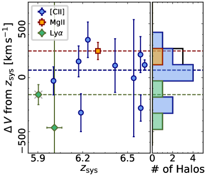
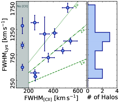
Figure 5: Left Panel — Velocity difference between the flux–weighted centroid of the nebular emission and the systemic redshift of the quasar (see Equation 3). Different symbols indicate different emission lines used to derive the quasar redshifts (i,e, blue points for [C ii] 158 $\mu$m, orange squares for Mg ii, and green diamonds for Ly$\alpha$, see section 2 for details). Horizontal dashed lines indicate the weighted average velocity difference of the different lines. The error–weighted average shift calculated for the entire sample is $\langle\Delta V_{\rm sys}\rangle=(+71\pm 31)$ km s^-1. This is shown as a black dashed line that overlaps with the average estimated from the [C ii] 158 $\mu$m redshifts only. The histograms on the left–hand side of this panel display the distribution of the shifts color–coded as on the right–hand side. Right Panel — Comparison between the FWHM of the detected extended Ly$\alpha$ emission (FWHM_Lyα) and of the [C ii] 158 $\mu$m line arising from the quasar’s host–galaxy (FWHM_C[II]). To guide the eye, green lines mark FWHM_Lyα that are 1, 2, and 3$\times$ wider than FWHM_C[II]. The wide distribution of the FWHM_Lyα (ranging from $\sim 250$ km s^-1 to $\sim 1750$ km s^-1) is apparent in the histogram on the left–hand side of this panel.
In both panels, gray crosses mark targets not part of our core sample (see section 2).

5.1.3 The SFR of the quasar host–galaxies

It is tempting to explore the possibility that the intense starbursts observed at mm–wavelengths directly influence the powering of the extended Ly$\alpha$ emission. SFR–based Ly$\alpha$ luminosities (${\rm L^{\rm SFR}_{\rm Ly\alpha}}$) are expected to follow the linear relation:

$$\frac{\rm L^{\rm SFR}_{\rm Ly\alpha}}{10^{42}\,{\rm erg\,s^{-1}}}=1.62\frac{\rm SFR}{\rm M_{\odot}\,yr^{-1}},$$ (4)

for which we assume the H$\alpha$ calibration relation (e.g., Kennicutt & Evans, 2012) and the case B recombination Ly$\alpha$–to–H$\alpha$ line ratio. Star formation rates can be derived either from the [C ii] 158 $\mu$m emission line or from rest frame far–infrared dust continuum luminosity of the quasar hosts. [C ii] 158 $\mu$m estimates, however, depend on the (unknown) dust metallicity, especially in the case of compact starbursts (e.g., De Looze et al., 2014). The dust continuum, on the other hand, can be used to estimate SFRs more directly by assuming that the dust is heated by star formation (i.e., considering that the quasar has a negligible contribution to the observed emission Leipski et al., 2014) and that the dust spectral energy distribution is well parameterized by a modified blackbody with a (typical) temperature of T${}_{\rm dust}=47$ K and a spectral index of $\beta=1.6$ (Beelen et al., 2006; Barnett et al., 2015). Conveniently, we detected the rest frame far–infrared dust continuum significantly for all quasars in our sample except J2228$+$0110. In the following, we will thus consider SFRs based on the dust continuum from Venemans et al. (2018 , and references therein). We stress that in high–$z$ quasar host–galaxies, SFRs derived from [C ii] 158 $\mu$m and from far–infrared continuum correlate, albeit with a large scatter (see discussion in, e.g., Decarli et al., 2018; Venemans et al., 2018).

Figure 6 shows that Ly$\alpha$ luminosities of the extended emission are broadly independent of the SFRs of the quasar host–galaxies and are typically well below the expectation based on Equation 4 (shown as a green dashed line). The resonant nature of the Ly$\alpha$ line with the large mass in dust present in the host–galaxies (M${}_{\rm dust}=10^{7}-10^{9}$ M_⊙, Venemans et al., 2018) are possible processes responsible for the suppression of the Ly$\alpha$ emission (e.g. Kunth et al., 1998; Verhamme et al., 2006; Gronwall et al., 2007; Atek et al., 2008; Sobral, & Matthee, 2019 ; see also Mechtley et al. 2012 for a study of the host galaxy of the $z\sim 6.4$ quasar J1148+5251). The cumulative effect can be quantified by the so–called Ly$\alpha$ escape fraction ($f_{\rm esc,Ly\alpha}$, e.g., Kennicutt & Evans, 2012). The median value of $f_{\rm esc,Ly\alpha}$ estimated for our sample is $\lesssim$1%. This is an order of magnitude lower than typically reported for $z\sim 6$ LAEs (e.g., Ono et al., 2010; Hayes et al., 2011) but consistent with the most massive, highly star–forming galaxies observed in the 3D–HST/CANDELS survey (Oyarzún et al., 2017). However, this value should be considered with some caution. The precise estimate of $f_{\rm esc,Ly\alpha}$ is strongly affected by different properties of the host galaxy (e.g., neutral hydrogen column density, neutral fraction, geometry, gas–to–dust ratio, etc., see Draine, 2011; Hennawi & Prochaska, 2013 ; and references therein) and by the patchiness of the dust cocoon (e.g., Casey et al., 2014). In addition, other mechanisms could contribute to the observed Ly$\alpha$ emission, in particular the presence of the strong radiation field generated by the quasar (e.g., Cantalupo et al., 2005 ; see also subsection 5.3).

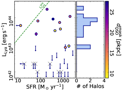
Figure 6: Total Ly$\alpha$ luminosity of the extended halos (L_Lyα, see Table 3) versus star formation rate derived from the dust continuum emission of the quasar host–galaxies (SFR). 3–$\sigma$ upper–limits on L_Lyα and on SFR are shown as downward and leftward arrows, respectively. Different colors show the value of $d^{\rm mask}_{\rm QSO}$ (see Table 2). The green dashed line indicates the unobscured Ly$\alpha$ emission expected from UV photons generated in intense starbursts, such as detected at mm–wavelengths (Equation 4). Most of the detected halos have L_Lyα below this prediction. Gray crosses represent quasars that are not part of our core sample (see section 2).

5.2 The kinematics of the gas

In Figure 4 we presented the two dimensional flux–weighted maps of the velocity centroid and dispersion distribution of the extended Ly$\alpha$ emission (see subsection 4.3 for details). In this section, we investigate these resolved kinematics maps in order to identify signatures of ordered motion, in/outflows, rotations, etc. We remind the reader that these maps were computed in a non–parametric way in the regions identified by ${\rm MASK_{x,y,\lambda}}$, and that velocity shifts are not relative to the quasar’s systemic redshift.

5.2.1 Velocity fields

The relatively low signal–to–noise of the first moment maps (see Figure 4) makes hard to infer the potential presence of ordered motion in the gas. In addition, due to the resonant nature of the Ly$\alpha$ line, the signature of coherent motion could be hindered by radiative transfer effects (e.g., Cantalupo et al., 2005). Indeed, the majority of the halos identified in the REQUIEM survey do not show evidence of rotation, as it was reported in extended Ly$\alpha$ halos at $z\sim 2-4$ (Borisova et al., 2016; Arrigoni Battaia et al., 2019a; Cai et al., 2019).

A noticeable exception is the nebular emission around the quasar P231$-$20. A velocity gradient can be seen ranging from $-200$ to $+800$ km s^-1 East to West (see Figure 7). Intriguingly, two [C ii] 158 $\mu$m–bright companions located within $\lesssim 14$ kpc from the quasar host galaxy have been discovered (Decarli et al., 2017; Neeleman et al., 2019). Both the velocity shear and the presence of a rich environment are reminiscent of the enormous Ly$\alpha$ nebular emission observed around the quasar SDSS J1020$+$1040 at $z=3.2$ by Arrigoni Battaia et al. (2018a) (albeit on a smaller scale). This system is considered a prototype to investigate the feasibility of inspiraling accretion onto a massive galaxy at $z\sim 3$. Indeed, simulations predict that baryons assemble in rotational structures, gaining angular momentum from their dark matters halos (e.g., Hoyle, 1951; Fall, & Efstathiou, 1980; Mo et al., 1998) and from accretion streams (e.g., Chen et al., 2003; Kereš et al., 2009; Kereš, & Hernquist, 2009; Brook et al., 2011; Stewart et al., 2017). In this scenario the cool accreting gas should be able to shape the central galaxy, delivering both fuel for star formation and angular momentum to the central regions (e.g., Sales et al., 2012; Bouché et al., 2013). High resolution ($\sim 0\farcs 35$) observations of the [C ii] 158 $\mu$m emission of the quasar host galaxy of P231$-$20 does not show a strong signature of rotation (Neeleman et al., 2019). This supports the idea that the system recently underwent a merger event with the close companion galaxy (located at a separation of 9 kpc and $-$135 km s^-1, Decarli et al., 2017; Neeleman et al., 2019) that perturbed the gas distribution.

If one assumes that the gas in the extended halo of P231$-$20 is (at first order) gravitationally bound, it is possible to approximate the dynamical mass of the system as $M_{\rm dyn}=1.16\times 10^{5}\,v_{\rm circ}\,d$ where $d$ is the diameter of the nebular emission in pkpc and $v_{\rm circ}$ its circular velocity in km s^-1. Given that the gas shows ordered motion, $v_{\rm circ}$ can be expressed as $v_{\rm circ}=0.75\,{\rm FWHM}_{\rm Ly\alpha}/\sin{i}$, with the (unknown) inclination typically considered to be $i=55^{\circ}$. This gives us a dynamical mass of $M_{\rm dyn}\sim 1.5\times 10^{13}$ M_⊙. Albeit the large uncertainties associated with this measurement, the estimated dynamical mass is remarkably similar to the mass predicted for the Ly$\alpha$ emission around the $z=2.28$ radio–quiet quasar UM287 (Cantalupo et al., 2014). Martin et al. (2015, 2019) interpreted this emission, which extends out to $\sim$500 kpc, as a large proto–galactic disc. Deeper MUSE observations are however necessary to fully capture the complex kinematics of this system.

The low incidence of clearly rotating structures in our sample is broadly in agreement with results by Dubois et al. (2012) who re–simulated two massive ($0.5$ and $2.5\times$10¹² M_⊙) $z\sim 6$ halos. They show that a significant fraction of the gas in the halo can fall almost radially towards the center. The reduced angular momentum inside the virial radius (mostly due to the isotropic distribution of the 0 and to gravitational instabilities and mergers, see also Prieto et al., 2015) allows for efficient funnelling of gas to the central regions of the halos, potentially sustaining the rapid growth of the first supermassive black holes.

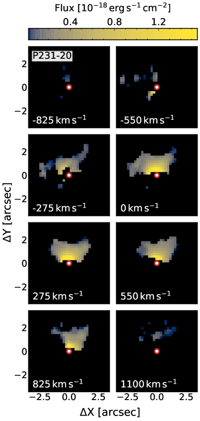
Figure 7: Velocity field of the extended Ly$\alpha$ nebular emission detected around the quasar P231$-$20 convolved with a 3D Gaussian kernel with $\sigma_{\rm spat}=0\farcs 2$ in the spatial and $\sigma_{\rm spec}=2.50$ Å in the spectral direction. Zero velocity is set to the [C ii] 158 $\mu$m redshift of the quasar ($z_{\rm sys}=6.5864\pm 0.0005$, while in Figure 4 velocity differences are relative to the flux–weighted centroid of the extended emission). The red circle in the center of each image marks the location of the quasar. Only voxels that are part of ${\rm MASK_{x,y,\lambda}}$ are shown. $\Delta X$ goes from East to West, $\Delta Y$ from South to North. The bulk of the emission is redshifted with respect to the quasar’s systemic redshift, and the nebula shows a velocity gradient going from East to West.

5.2.2 Velocity dispersion

The second–moment maps presented in Figure 4 show that the detected extended Ly$\alpha$ halos have average flux–weighted velocity dispersions ($\langle\sigma_{\rm Ly\alpha}\rangle$) spanning from $\langle\sigma_{\rm Ly\alpha}\rangle\sim 30$ km s^-1 to $460$ km s^-1 with an average of $320\pm 120$ km s^-1. Note that these values have been corrected for the limited spectral resolution of MUSE according to: $\left(\sigma_{\rm Ly\alpha}^{\rm corr}\right)^{2}=\left(\sigma_{\rm Ly\alpha}^{\rm meas.}\right)^{2}-\left(\sigma_{\rm Res.}^{\lambda}\right)^{2}$, where $\sigma_{\rm Res.}^{\lambda}\sim 35$ km s^-1 at the wavelengths explored in our sample. The relatively quiescent $\langle\sigma_{\rm Ly\alpha}\rangle$ values are consistent with measurements reported by Borisova et al. (2016), Arrigoni Battaia et al. (2019a), and Cai et al. (2019) around bright $z\sim 2-4$ quasars.

At $z\sim 3.7$ Borisova et al. (2016) reported a larger velocity dispersion ($\langle\sigma_{\rm ly\alpha}\rangle>400$ km s^-1) for a halo around a radio–loud quasar than for halos around radio–quiet quasars. In the REQUIEM sample there is one radio–loud quasar, J2228$+$0110. It shows a flux–weighted velocity dispersion of ($350\pm 90$) km s^-1, in agreement with the rest of our (radio–quiet) sample. This dispersion is consistent with Arrigoni Battaia et al. (2019a), who derived similar kinematics for nebulae around radio–loud and radio–quiet quasars at $z\sim 3.2$

Ginolfi et al. (2018) suggested that the high velocity dispersions observed for the Ly$\alpha$ extended emission around the broad–absorption line quasar J1605$-$0112 at $z=4.9$ could be linked to an outflow of material escaping the central black hole. Our sample contains only one broad–absorption line quasar (J2216$-$0016) that is 2.9 mag fainter than J1605$-$0112. For this object we do not detect the presence of any significant extended emission. Given the generally quiescent motion of the nebulae in our sample, it is unlikely we are probing fast outflows driven by the quasar (expected to be of the order of $\gtrsim 1000$ km s^-1, e.g., Tremonti et al., 2007; Villar-Martín, 2007; Greene et al., 2012). Nonetheless, we cannot exclude this scenario for the halos associated with the quasars P065$-$26 and P340$-$18, where the observed gas velocities are of the order ${\rm FWHM}\gtrsim 1500$ km s^-1. Simulations of luminous ($>{\rm few}\times 10^{46}$ erg s^-1) quasars indeed predict AGN–driven winds with such large velocities, however these could happen at different scales, from less than 1 kpc to several tens (e.g., Costa et al., 2015; Bieri et al., 2017). However, given the current spatial resolution of our data, we are not sensitive to the presence of extreme kinematics on scales $\lesssim 5$ kpc (where the such an emission would be diluted by the flux of the central AGN).

Is the gas gravitationally bound to the halo? Recent observations (both in absorption and in emission) of the gas in the circum–galactic medium of quasars have revealed velocity dispersions consistent with the gravitational motion within dark matter halos with masses ${\rm M}_{\rm DM}\gtrsim 10^{12.5}$ M_⊙ (e.g., Prochaska, & Hennawi, 2009; Lau et al., 2018; Arrigoni Battaia et al., 2019a). These are typical masses of halos hosting quasars, derived from strong quasar–quasar and quasar–galaxy clustering observed out to $z\sim 4$ (e.g., Shen et al., 2007; White et al., 2012; Eftekharzadeh et al., 2015; García-Vergara et al., 2017; Timlin et al., 2018; He et al., 2018). At $z\sim 6$, however, such a direct measurement still eludes us. Nevertheless, we can gain some insight by comparing the number density of bright quasars and massive dark matter halos (e.g., Shankar et al., 2010), under the assumption that there is a correlation between the luminosity (mass) of a quasar and the mass of the dark matter halo it is embed in (see e.g., Volonteri et al., 2011). By integrating the Kashikawa et al. (2015) luminosity function at $z=6.3$ (i.e., the average redshift of our survey), we can expect a number density of $\phi\left({\rm M}_{\rm 1450}<-25.25\right)=2.5\times 10^{-9}$ Mpc^-3 for quasars brighter than ${\rm M}_{\rm 1450}=-25.25$ mag. If we assume a high duty cycle of $f_{\rm duty}=0.9$ (as predicted by Shankar et al., 2010), we can infer that the integral of the halo mass function from Behroozi et al. (2013) matches the integral of the luminosity function for masses ${\rm M}_{\rm DM}\sim 10^{12.8}$ M_⊙.

We can now compare this value to the masses derived from the velocity dispersions observed in the detected halos. Indeed, if we assume an NFW (Navarro, Frenk, & White, 1997) density profile and the concentration–mass relation presented in Dutton & Macciò (2014), the 1D root–mean–square velocity dispersion ($\sigma^{\rm rms}_{\rm 1D}$) can be directly related with the maximum circular velocity ($V^{\rm Max}_{\rm circ}$) as: $\sigma_{\rm 1D}=V^{\rm Max}_{\rm circ}/\sqrt{2}$ (Tormen et al., 1997). The average $\sigma^{\rm rms}_{\rm 1D}$ in the REQUIEM sample is $\langle\sigma^{\rm rms}_{\rm 1D}\rangle=\left(340\pm 125\right)$ km s^-1, consistent with the gravitational motion in a ${\rm M_{\rm DM}}\sim 10^{12.5}$ M_⊙ halo at $z=6$ (see Figure 8). Although most of the detected nebulae are associated with quasars confined to a narrow luminosity range (i.e., between ${\rm M}_{\rm 1450}\sim-26$ mag and $-27.5$ mag), no clear dependency between the velocity dispersion of the nebulae and ${\rm M}_{\rm 1450}$ is observed (see Figure 8). This suggests that the mechanisms responsible for the broadening of the Ly$\alpha$ line do not depend on the rest–frame UV emission of the central super–massive black hole.

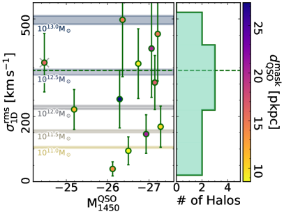
Figure 8: 1D root–mean–square velocity dispersion measured in each detected nebulosity ($\sigma^{\rm rms}_{\rm 1D}$) versus the monochromatic luminosity of the quasars ($M_{\rm 1450}^{\rm QSO}$). Points are color–coded by the size of the recovered halo ($d_{\rm QSO}^{\rm mask}$). Horizontal bands are velocity dispersions expected for NFW dark matter halos with masses ranging from 10¹¹ to 10¹³ M_⊙. Lower and upper limits of each band correspond to estimates at $z=5.9$ and $z=6.6$, respectively. Despite the large scatter, the average velocity dispersion of the nebulae (plotted as a green dashed line) is consistent with values expected in a $z\sim 6$ dark matter halo of ${\rm M}_{\rm DM}\sim 10^{12.5}$ M_⊙.

5.3 The powering mechanism(s) of the extended halos

The currently favored mechanism to explain the extended emission observed around quasars is Ly$\alpha$ fluorescence, i.e., the recombination emission following photoionization of cool ($T\sim 10^{4}$ K) gas by the strong quasar radiation field (e.g., Hennawi & Prochaska, 2013; Arrigoni Battaia et al., 2016, 2019a; Cantalupo, 2017). In general, if we assume that quasars are surrounded by a population of cool spherical gas clouds, we can directly infer the surface brightness of the fluorescence emission in two limiting regimes:

• The gas in the clouds is optically–thick (i.e., with $N_{\rm HI}\gg 10^{17.2}$ cm^-2). In this case it is able to self–shield from the quasar’s radiation and the Ly$\alpha$ emission originates from a thin, highly ionized envelope around each individual cloud;

• The gas is optically thin (i.e., with $N_{\rm HI}\ll 10^{17.2}$ cm^-2) and it is maintained in a highly ionized state by the quasar radiation. In this case, the Ly$\alpha$ emission originates from the entire volume of each cloud.

In the following we will exploit the formalism presented in Hennawi & Prochaska (2013) to gain insight into the physical status of the gas surrounding the first quasars.

5.3.1 Optically thick scenario

If the gas is optically thick, the Ly$\alpha$ surface brightness of the extended emission is expected to be proportional to the flux of ionizing photons coming from the central AGN ($\Phi$), to the covering fraction of optically thick clouds ($f^{\rm thick}_{\rm C}$), and to the fraction of incident photons converted into Ly$\alpha$ by the cloud’s envelope ($\eta_{\rm thick}$, see also Hennawi et al., 2015; Farina et al., 2017; Cantalupo, 2017):

$${\rm SB^{\rm thick}_{Ly\alpha}}=\frac{\eta_{\rm thick}h\nu_{\rm Ly\alpha}}{4\pi\left(1+z\right)^{4}}f^{\rm thick}_{\rm C}\Phi\left(\frac{R}{\sqrt{3}}\right),$$ (5)

where we considered the cool gas clouds to be spatially uniformly distributed in a spherical halo of radius $R$. $\Phi$ can be expressed as a function of the luminosity of the quasar as:

$$\Phi\left(r\right)=\int_{\nu_{\rm LL}}^{\infty}\frac{F_{\nu}}{h\nu}d\nu=\frac{L_{\nu_{\rm LL}}}{4\pi r^{2}}\int_{\nu_{\rm LL}}^{\infty}\frac{1}{h\nu}\left(\frac{\nu}{\nu_{\rm LL}}\right)^{\alpha_{\rm UV}}d\nu,$$ (6)

where we considered that, blueward of the Lyman limit ($\nu_{\rm LL}$) the quasar spectral energy distribution has the form $L_{\nu}=L_{\nu_{\rm LL}}\left(\nu/\nu_{\rm LL}\right)^{\alpha_{\rm UV}}$ with $\alpha_{\rm UV}=-1.7$. The luminosity at the Lyman edge ($L_{\nu_{\rm LL}}$) can be directly derived from ${\rm M}_{\rm 1450}$ as: ${\rm M}_{912}={\rm M}_{\rm 1450}+0.33$ (see Lusso et al., 2015). Considering $\eta_{\rm thick}=0.66$, we can thus write:

$$\frac{{\rm SB}_{\rm Ly\alpha}^{\rm thick}}{10^{-17}{\rm erg\,s^{-1}\,cm^{-2}\,arcsec^{-2}}}=21.0\left(\frac{1+z}{1+6.2}\right)^{-4}\times\\ \times\left(\frac{f_{\rm C}^{\rm thick}}{0.5}\right)\left(\frac{R}{20\,{\rm pkpc}}\right)^{-2}\left(\frac{L_{\nu_{\rm LL}}}{10^{31}\,{\rm erg\,s^{-1}\,Hz^{-1}}}\right).$$ (7)

Considering that our core sample has an average luminosity at the Lyman edge of $\langle L_{\nu_{\rm LL}}\rangle=2\times 10^{31}$ erg s^-1 Hz, the optically thick scenario predicts a surface brightness of ${\rm SB}_{\rm Ly\alpha}^{\rm thick}\sim 40\times 10^{-17}$ erg s^-1 cm^-2 arcsec^-2, i.e. $\gtrsim 2$ orders of magnitude higher than observed (see Figure 9). Despite the presence of unknowns such as the geometry of the quasar emission or the covering fraction of optically thick clouds (that may be of the order of 60% within a projected distance of 200 pkpc from $z\sim 2-3$ quasars, e.g. Prochaska et al., 2013a), this discrepancy points to a different scenario for the origin of the extended Ly$\alpha$ emission. The optically thick regime is also disfavored by the absence of a clear correlation between ${\rm SB}_{\rm Ly\alpha}$ and $L_{\nu_{\rm LL}}$ (and thus ${\rm M}_{\rm 1450}$) as expected from Equation 7 (see Figure 9).

5.3.2 Optically thin scenario

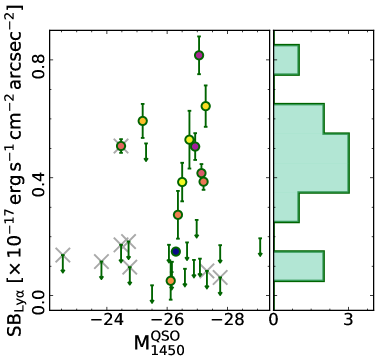
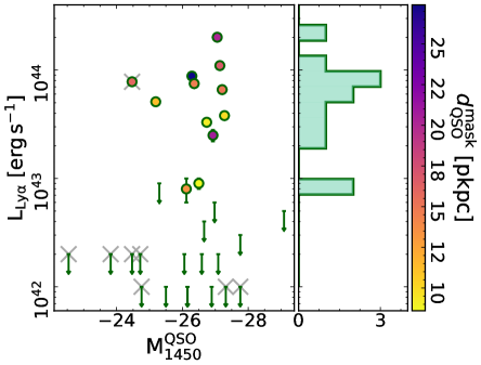
Figure 9: Left Panel — Average surface brightness versus ${\rm M}_{\rm 1450}$. $3-\sigma$ upper–limits for non–detected nebulae are shown as downward arrows. The colormap of the points is the same as in Figure 6. For consistency with subsection 4.2, here the average ${\rm SB}_{\rm Ly\alpha}$ is calculated using a circular aperture of radius $d_{\rm QSO}^{\rm mask}$ (or 20 pkpc if the halo was not detected) on pseudo–narrow–band images obtained collapsing the datacube between $\pm 500$ km s^-1 relative to the quasar’s systemic redshift. Targets not part of our core sample are marked with gray crosses (see section 2). Right Panel — Same as the left panel but with the total Ly$\alpha$ luminosity of the extended halo as $y$–axis.

If the quasar radiation is sufficiently intense to keep the gas highly ionized (i.e. if the neutral fraction $x_{\rm HI}=n_{\rm HI}/n_{\rm H}\ll 1$), the expected average surface brightness arising from these optically thin clouds is independent of the quasar luminosity and can be expressed as:

$$\frac{{\rm SB}_{\rm Ly\alpha}^{\rm thin}}{10^{-19}{\rm erg\,s^{-1}\,cm^{-2}\,arcsec^{-2}}}=3.6\left(\frac{1+z}{1+6.2}\right)^{-4}\times\\ \times\left(\frac{f_{\rm C}^{\rm thin}}{0.5}\right)\left(\frac{n_{\rm H}}{1\,{\rm cm^{-3}}}\right)\left(\frac{N_{\rm H}}{10^{20.5}\,{\rm cm^{-2}}}\right),$$ (8)

where $f^{\rm thin}_{\rm C}$ is the covering fraction of optically thin clouds, and $n_{\rm H}$ and $N_{\rm H}$ are the cloud’s hydrogen volume and column densities, respectively (see Osterbrock, & Ferland, 2006; Gould & Weinberg, 1996; Hennawi & Prochaska, 2013 for further details). Assuming photoionization equilibrium allows us to express the neutral column density averaged over the area of the halo ($\langle N_{\rm HI}\rangle$) in terms of $L_{\nu_{\rm LL}}$ and $L_{\rm Ly\alpha}$:

$$\frac{\langle N_{\rm HI}\rangle}{10^{17.2}\,{\rm cm}^{-2}}=0.1\left(\frac{L_{\rm Ly\alpha}}{10^{44}\,{\rm erg\,s^{-1}}}\right)\times\\ \times\left(\frac{L_{\nu_{\rm LL}}}{10^{31}\,{\rm erg\,s^{-1}\,Hz^{-1}}}\right)^{-1}.$$ (9)

Given the observed luminosities of the nebulae in our core sample ($L_{\rm Ly\alpha}\lesssim 10^{44}$ erg s^-1, see Table 3) we obtain $\langle N_{\rm HI}\rangle\ll 10^{17.2}$ cm^-2, consistent with the optically thin regime. However, we stress that $\langle N_{\rm HI}\rangle$ is obtained by averaging over the whole area of the halo. So, while $\langle N_{\rm HI}\rangle\gg 10^{17.2}$ cm^-2 definitively determines the clouds to be optically thick, a small value of $\langle N_{\rm HI}\rangle$ does not provide the same clear result, since individual clouds may still be optically thick while being surrounded by a thinner medium.

Under the assumption that the clouds are optically thin, it is of interest to use Equation 8 to derive constraints on the gas volume density ($n_{\rm H}$). Studies of absorption systems associated with gas surrounding $z\sim 2$ quasars suggest that $N_{\rm H}$ is almost constant within an impact parameter 200 pkpc at a median value of $N_{\rm H}=10^{20.5}$ cm^-2 (e.g. Lau et al., 2016). If $z\sim 6$ quasars are embedded in halos with similar hydrogen column densities, our observations imply $n_{\rm H}>1$ cm^-3. Intriguingly, similarly high gas densities have been invoked to explain the Ly$\alpha$ emission in giant nebulae discovered around $z\sim 2-3$ quasars (Cantalupo et al., 2014; Hennawi et al., 2015; Arrigoni Battaia et al., 2015b, 2018a; Cai et al., 2018).

5.3.3 Other possibilities

In addition, other mechanisms have been proposed to explain the presence of extended Ly$\alpha$ nebulae including gravitational cooling radiation (e.g., Haiman et al., 2000; Fardal et al., 2001; Furlanetto et al., 2005; Dijkstra, & Loeb, 2009), shocks powered by outflows (e.g., Taniguchi, & Shioya, 2000; Mori et al., 2004), or resonant scattering of Ly$\alpha$ photons (e.g. Gould & Weinberg, 1996; Dijkstra, & Loeb, 2008).

However, Ly$\alpha$ emission coefficients for collisional excitation are exponentially dependent on the temperature (Osterbrock, & Ferland, 2006). The concurrence of a very narrow density and temperature range for all the gas in every observed Ly$\alpha$ nebula would thus be necessary to validate this. Instead, recombination radiation has a much weaker dependence on temperature (Osterbrock, & Ferland, 2006), providing a more natural explanation for the Ly$\alpha$ extended emission in the presence of a strong ionizing flux (e.g., Borisova et al., 2016). In addition, the relatively quiescent motion of the gas in the detected halos (see subsection 5.2) is not easily reconciled with shock–powered emission (see also discussion in Arrigoni Battaia et al., 2019a).

On the other hand, resonant scattering of Ly$\alpha$ photons from the central AGNs and from young stars in the host galaxies can provide a relevant contribution to the emission, if the gas is optically thick at the Ly$\alpha$ transition ($N_{\rm HI}\gtrsim 10^{14}$ cm^-2). This was proposed as the main process powering the extended Ly$\alpha$ emission detected around $3\lesssim z\lesssim 6$ Ly$\alpha$ emitters by Wisotzki et al. (2016). Hennawi & Prochaska (2013) showed that the surface brightness of extended Ly$\alpha$ emission produced via resonant scattering by neutral gas in the CGM (${\rm SB}_{\rm Ly\alpha}^{\rm scatt.}$) is expected to be directly proportional to the flux of ionizing photons emitted close to the Ly$\alpha$ resonance ($L_{\rm\nu Ly\alpha}$). Given that the peak of the Ly$\alpha$ line of $z\sim 6$ quasars is typically absorbed by neutral hydrogen, there is no direct way to test for the presence of such a correlation in the REQUIEM survey. In any case, Arrigoni Battaia et al. (2019a) reported the lack of significant correlation between the surface brightness of Ly$\alpha$ halos and the luminosity of the peak of the Ly$\alpha$ line of $z\sim 3$ quasars. In addition, we do not detect clear signals of the characteristic double–peaked profiles expected for resonantly trapped Ly$\alpha$ photons (e.g., Dijkstra, 2017). However, a detailed analysis of the Ly$\alpha$ line shape performed on high signal–to–noise, high spectral resolution spectra is required to properly test this scenario.

We stress that all the aforementioned mechanisms can be in place at the same time and contribute at different levels to the observed emission. Additional factors can also modulate the total luminosity of the halos. For instance, the presence of dust on scales larger than 20 kpc (e.g. Roussel et al., 2010; Ménard et al., 2010) can destroy Ly$\alpha$ photons, and/or the variability of the quasar emission (e.g., MacLeod et al., 2012; Yang et al., 2019) can be faster than the response of the halo (with a strong dependence on $n_{\rm H}$) and wash out some of the expected correlations. Future observations of non–resonant lines such as He ii or H$\alpha$ will be instrumental in disentangling different emission mechanisms (e.g. Arrigoni Battaia et al., 2015b; Leibler et al., 2018; Cantalupo et al., 2019). This is particularly challenging at $z>6$, where only space–based observations will have the sensitivity necessary to provide additional information about the gas surrounding the first quasars.

5.4 Ly$\alpha$ nebulae and galaxy overdensities

Several giant Ly$\alpha$ nebulae extending on scales $\gg 100$ kpc have recently been reported in the literature (Cantalupo et al., 2014; Hennawi et al., 2015; Cai et al., 2018; Arrigoni Battaia et al., 2018a, 2019b; Lusso et al., 2019). The incidence of such large nebulae has been estimated to be of the order of few percent at $z\sim 2-3$ (Hennawi & Prochaska, 2013; Arrigoni Battaia et al., 2016, 2019a). A larger sample of $z\gtrsim 6$ quasars is necessary to assess if this low occurrence holds at high redshifts. In any case, all $z<4$ giant nebulae appear to be invariably associated with overdensities of AGN and galaxies, suggesting a connection between proto–cluster structures and extremely extended emission (e.g., Hennawi et al., 2015; Arrigoni Battaia et al., 2018b , but see Bădescu et al. 2017 for examples of large Ly$\alpha$ blobs located at the outskirts of high–density regions).

We can qualitatively test this scenario at $z>6$, by searching for peculiarities in the nebulae associated with quasars for which deep ALMA observations have revealed the presence of bright [C ii] 158 $\mu$m companions (i.e., J0305$-$3150, P231$-$20, P308$-$21, and J2100$-$1715; see section 2 and Decarli et al., 2017; Willott et al., 2017; Venemans et al., 2019). J2100$-$1715 has a [C ii] 158 $\mu$m companion located at a separation of $\sim 60$ kpc (Decarli et al., 2017; Neeleman et al., 2019) but does not show the presence of any significant extended Ly$\alpha$ emission. J0305$-$3150, although located in an overdensity with three [C ii] 158 $\mu$m and one LAE emitter (Farina et al., 2017; Venemans et al., 2019), shows a really faint halo. Finally, P231$-$20 and P308$-$21 host among the brightest and most extended halos in the REQUIEM survey and both are in the middle of gravitational interactions with their companions (Decarli et al., 2019b; Neeleman et al., 2019).

The variety of the Ly$\alpha$ emission observed in this (small) sample of quasars with companions suggests that at $z>6$, bright and extended Ly$\alpha$ halos may be associated with ongoing merger events. If this is the case, P323$+$12, that exhibits the brightest nebular emission in our sample, is likely to be in a gravitational interaction. Mazzucchelli et al. (2017) presented low resolution NOEMA observations on the [C ii] 158 $\mu$m emission line of this source, without detecting a merger. However testing the merger scenario requires a higher sensitivity and better spatial resolution, for example with ALMA or NOEMA.

5.5 The average surface–brightness profile

In this section we will infer the average surface brightness profile of the Ly$\alpha$ emission around quasars in the REQUIEM survey and we will compare its shape with lower redshift studies. To avoid selection effects, we will focus only on our core sample. We remind the reader that this consists of 23 radio–quiet quasars at an average redshift of $\langle z\rangle=6.27$ and absolute magnitude ranging from ${\rm M}_{\rm 1450}=-25.2$ mag to $-29.1$ mag, with an average of $\langle{\rm M}_{\rm 1450}\rangle=-27.1$ mag (see section 2). As a lower redshift comparison we will use the following studies (see Figure 10): (i) Cai et al. (2019), who investigated with KCWI 16 quasars at $2.20<z<2.38$ (with an average of $\langle z\rangle=2.27$) and absolute magnitude between ${\rm M}_{\rm 1450}=-29.0$ mag and $-26.1$ mag (with $\langle{\rm M}_{\rm 1450}\rangle=-27.3$ mag); (ii) QSO MUSEUM (Arrigoni Battaia et al., 2019a), a MUSE investigation for extended Ly$\alpha$ emission around a sample of 61 quasars at $3.03<z<3.46$ (with $\langle z\rangle=3.21$) with absolute magnitudes in the range $-28.3\,{\rm mag}<{\rm M}_{\rm 1450}<-25.6$ mag (with $\langle{\rm M}_{\rm 1450}\rangle=-27.2$ mag); and (iii) Borisova et al. (2016), who explored with MUSE the vicinity of 19 bright ($-29.0\,{\rm mag}<M1450<-26.8\,{\rm mag}$, and $\langle{\rm M}_{\rm 1450}\rangle=-28.0$ mag) quasars at $3.02<z<3.91$ (with $\langle z\rangle=3.36$).

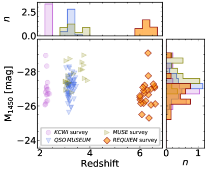
Figure 10: Redshift vs. ${\rm M}_{\rm 1450}$ distribution of the quasars part of the surveys from Cai et al. (2019 , 16 quasars, magenta circles and histograms), Arrigoni Battaia et al. (2019a , 61 quasars, light blue down–pointing triangles and histograms), and Borisova et al. (2016 , green right–pointing triangles and histograms). The 23 quasars part of our core sample are shown as orange diamonds and histograms. Histograms are normalized by the total number of targets and by the bin size (with steps $0.3$ in redshift and of $0.3$ mag in absolute magnitude). The average absolute magnitude of the Cai et al., Arrigoni Battaia et al., and our core sample are nearly identical, while the quasars studies in Borisova et al. are, in average, $\sim 0.7$ mag brighter.

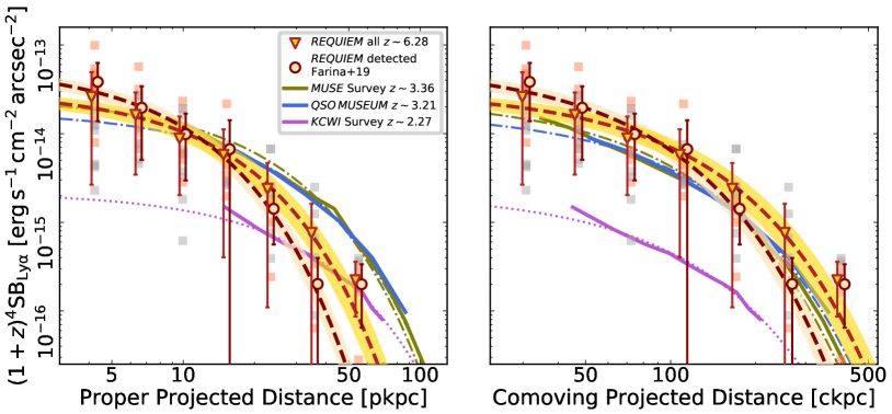
Figure 11: Left Panel – Average Ly$\alpha$ surface brightness profile of the core sample of our REQUIEM survey. We show the individual circularly–averaged profiles extracted around each quasar as orange squares for detected halos and gray squares for non–detections. Sum–averaged profiles considering all quasars (orange triangles) or only significantly detected halos (purple circles) are also shown, together with their respective best exponential fit (orange and purple dashed lines, shaded regions provide 1–$\sigma$ uncertainties in the fit). Data–points have been slightly shifted along the $x$–axis for the sake of clarity. The average surface brightness profile of the extended emission around quasars at $z\sim 2.27$ (magenta line, Cai et al., 2019), $z\sim 3.21$ (light blue line, Arrigoni Battaia et al., 2019a), and $z\sim 3.36$ (olive green line, Marino et al., 2019) are also plotted. The corresponding exponential best fits are shown in the same color palette. Note that all measurements are corrected for the $(1+z)^{4}$ factor to compensate for cosmological dimming. Right Panel – Same of Left Panel, but in comoving units.

The extended nebulae detected in the REQUIEM survey appear to have complex morphologies and clear asymmetries (see Figure 2). We proceeded following the standard approach in the literature and we obtained the surface brightness profiles averaging over circular apertures centered on the location of the quasars. As explained in subsection 4.2, single profiles were extracted from pseudo–narrow band images created by collapsing the datacubes over 30 Å centered at the location of the Ly$\alpha$ line, redshifted to the quasar’s systemic redshift. To create the stacked profile, we first correct these profiles for cosmological dimming (i.e., by a factor $(1+z)^{4}$) and then we average over them with equal weights. This prevents the introduction of biases towards deeper exposures and/or brighter objects (the marginal variations caused by the use of the median to combine the different radial profiles is discussed in Appendix D). We also create the stacked profile only using the sub–sample of quasars for which an extended emission has been detected with significance. The results of this procedure are plotted in Figure 11, where the average surface brightness profile obtained for all quasars is shown as orange triangles and the one from quasars embedded in halos as purple circles (the average radial profile for the entire core sample is tabulated in Table 4 in Appendix D). For comparison, the average profile from Cai et al. (2019), Arrigoni Battaia et al. (2019a), and Marino et al. (2019) are displayed as magenta, light blue, and olive solid lines, respectively.

In order to extract information from the stacked profiles, we perform a fit with an exponential function: $(1+z)^{4}\,{\rm SB}_{\rm Ly\alpha}\left(r\right)=C\exp{\left(-r/r_{h}\right)}$, where $C$ is the normalization and $r_{h}$ is the scale length of the profile. The resulting parameters are $C=(3.0\pm 0.4)\times 10^{-14}$ erg s^-1 cm^-2 arcsec^-2 and $r_{h}=(9.4\pm 0.8)$ kpc for the full sample and $C=(5.6\pm 0.8)\times 10^{-14}$ erg s^-1 cm^-2 arcsec^-2 and $r_{h}=(6.4\pm 0.3)$ kpc for the stack quasars with detected halos. As expected, while the two profile match within the errors, the latter appears slightly more concentrated due to the stronger signal in the central $\sim 20$ kpc. In the following, we will keep showing both profiles, however in the discussion we will focus solely on the one that includes all quasars as it is more representative of the full high–$z$ quasar population.

The scale length derived for $z\sim 6.2$ quasars is a factor of $\sim 2\times$ smaller than the $r_{h}=(15.5\pm 0.5)$ pkpc and $r_{h}=(21.1\pm 0.9)$ pkpc measured for radio–quiet quasars at $z\sim 3.2$ (Arrigoni Battaia et al., 2019a) and at $z\sim 2.3$ (Cai et al., 2019), suggesting that extended halos are more compact at higher redshift. For comparison, the sample of Ly$\alpha$ emitters in the Hubble Ultra Deep Field shows a much milder evolution of halo scale length, increasing from $r_{h}=(3.8\pm 1.3)$ pkpc at $5<z\lesssim 6$ to $r_{h}=(4.4\pm 1.5)$ pkpc at $3\lesssim z<4$ (Leclercq et al., 2017). However, we should note that, given the difference in apparent brightness of the quasars, the cosmological evolution of the angular diameter distance, and the factor $\sim 8\times$ in sensitivity due to redshift dimming, our observations are more sensitive to regions closer to the quasar while Cai et al. (2019), Arrigoni Battaia et al. (2019a), and Borisova et al. (2016) are more sensitive to extended emission at larger scales.

Arrigoni Battaia et al. (2019a) reported a strong evolution of the average properties of the extended emission with cosmic time. This was based on the comparison of the average surface brightness radial profiles of their quasars split into a $z\sim 3.3$ and a $z\sim 3.1$ sub–samples and the results obtained from a narrow–band survey of bright radio–quiet quasars at $z\sim 2.2$ (Arrigoni Battaia et al., 2016). Recently, Cai et al. (2019) showed that studies based on narrow–band imaging underestimated the total nebular emission of an order of magnitude (see also Discussion in Borisova et al., 2016). The new IFU observations revealed a less pronounced evolution, with halos surrounding quasars at $z\sim 2$ being $\sim 0.4$ dex fainter than at $z\sim 3$ (Cai et al., 2019). In the following, we will test if this trend holds out to the redshifts provided by the REQUIEM survey.

In the optically thin scenario, the Ly$\alpha$ surface brightness scales as ${\rm SB_{Ly\alpha}}\propto n_{\rm H}N_{\rm H}$ (see Equation 8). If the gas clouds are bound to the dark matter halo hosting the quasar (see subsection 5.2), it can be shown that $N_{\rm H}\propto n_{\rm H}R_{\rm vir}$, where $R_{\rm vir}$ is the virial radius (see also Churchill et al., 2013b , for a similar argument applied to Mg ii absorbers in the CGM of $z<1$ galaxies). In addition, given the inferred high densities ($n_{\rm H}>1$ cm^-3), the emitting gas is not likely to trace the evolution of the cosmic mean density. We thus expect the size of the nebular emission to scale with the growth of $R_{\rm vir}$ with cosmic times. For the sake of simplicity, we will consider that quasars are hosted by massive halos with $M_{\rm DM}=10^{12.5}$ M_⊙ independent of their redshift (see, e.g., discussion in Shen et al., 2007; He et al., 2018). Thus the virial radius $R_{\rm vir}\left(z\right)=\left[3M_{\rm DM}/4\pi\rho_{\rm c}\left(z\right)\right]^{\frac{1}{3}}$ depends only on the critical density of the Universe as a determined redshift [$\rho_{\rm c}\left(z\right)$]. For the considered halo, the virial radius calculated at $z=6.28$ increases of a factor $\sim 1.6\times$ down to $z=3.36$ and of a factor $\sim 2.2\times$ down to $z=2.27$.

In Figure 12 we show the average surface brightness profiles at $z=6.28$, $3.36$, $3.34$, $3.11$, and $2.27$ normalized by the virial radius. At all the these redshifts, the emitting gas appears to be located well within $R_{\rm vir}$ and the average profile becomes brighter at higher redshifts (with the $z\sim 3$ and $z\sim 6$ profiles being consistent within the scatter). If we model the profiles normalized by the virial radius with an exponential function: $(1+z)^{4}\,{\rm SB}_{\rm Ly\alpha}\left(r\right)=C_{h}\exp{\left(-x/x_{h}\right)}$ with $C_{h}$ and $x_{h}$ as free parameters and $x=r/R_{\rm vir}$, we obtain: $C_{h}=(3.0\pm 0.4)\times 10^{-14}$ erg s^-1 cm^-2 arcsec^-2 and $x_{h}=(0.15\pm 0.01)$ for the full quasar sample and $C_{h}=(5.6\pm 0.8)\times 10^{-14}$ erg s^-1 cm^-2 arcsec^-2 and $x_{h}=(0.13\pm 0.01)$ kpc for the sub–sample of detected halos. The value of $x_{h}$ measured at $z\sim 6.28$ matches the $x_{h}=0.14$, $0.16$, $0.15$, and $0.16$ estimated for quasars at $z\sim 3.36$, $z\sim 3.34$, $z\sim 3.11$, and $z\sim 2.27$ respectively. This suggests a scenario where the (average properties of the) extended Ly$\alpha$ emission mirrors the cosmic evolution of the dark matter halos they reside in (see also subsection 5.2). On the other hand, $C_{h}$ rapidly increases with redshift from $z\sim 2$ to $z\sim 3$ and grows much gradually between $z\sim 3$ and $z\sim 6$. This behavior is described by the gray dashed line in Figure 12. This is the expected average profile of the extended emission if the increase of the normalization observed between $z\sim 2.27$ and $z\sim 3.36$ would keep its pace linearly with redshift up to $z\sim 6.28$. The observed profile from the REQUIEM survey lies $\sim 0.4$ dex below this prediction.

Intriguingly, hydrodynamical cosmological simulations show that high–$z$ galaxies in dark matter halos of $M_{\rm DM}\gtrsim 10^{12}$ M_⊙ are mainly fed by cool gas streams (co–existing with a hot, shocked medium) down to redshift $z\sim 2-3$. Below this “critical” redshift, these cool streams are not able to balance the virial shock–heating and are suppressed (e.g., Dekel, & Birnboim, 2006; Dekel et al., 2009, 2019). This theoretical picture would naturally explain the observed evolution of the surface brightness profile. Under the assumption that the emission arises from optically thin clouds of gas, the surface brightness is expected to scale as: ${\rm SB_{Ly\alpha}}\propto(1+z)^{4}f_{\rm C}^{\rm thin}n_{\rm H}N_{\rm H}$ and $N_{\rm H}$ is proportional to the total mass in cool gas $M_{\rm cool}$ (see subsection 5.3 and Hennawi & Prochaska, 2013; Arrigoni Battaia et al., 2019a). Thus, the small variation in Ly$\alpha$ surface brightness reported between $z\sim 6$ and $z\sim 3$ suggests that cool streams are able to replenish the CGM with gas, permitting $M_{\rm cool}$ to keep pace with $M_{\rm DM}$. The consequent heating of massive halos at $z\lesssim 3$ may be responsible for the drop of cool gas in the CGM and, thus, of the average Ly$\alpha$ emission. However, this picture clashes with the large amount of cool gas revealed by absorption studies of the CGM around $0.5\lesssim z\lesssim 2$ quasars (e.g., Bowen et al., 2006; Farina et al., 2013, 2014; Prochaska et al., 2014; Johnson et al., 2015).

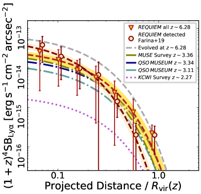
Figure 12: Average, cosmological dimming corrected, surface brightness profiles of the extended emission around quasars with the radius normalized to the virial radius R${}_{vir}\left(z\right)$ of a $10^{12.5}$ M_⊙ dark matter halo located at different redshifts. The color code of data–points and curves is the same as in Figure 11. In addition, following Arrigoni Battaia et al. (2019a), we split quasars part of the QSO MUSEUM in two sub–samples with median redshifts $z=3.11$ and $z=3.34$. The corresponding exponential fit of the surface brightness profiles are plot as light and dark blue dashed–dotted line, respectively. The gray dashed line shows the expected profile if the evolutionary trend observed between $z=2.27$ and $z=3.36$ is extrapolated linearly in redshift to $z=6.28$.

5.6 Extended emission and quasar near zones

Near the end of the cosmic reionization epoch, the large fraction of neutral hydrogen present in the Universe suppresses virtually all the emission blueward of the Ly$\alpha$ line (e.g., Gunn & Peterson, 1965). However, the intense radiation of a luminous quasar is able to ionize the surrounding gas, creating a bubble of enhanced transmission in the Ly$\alpha$ forest in its immediate vicinity known as the proximity (or near) zone (e.g., Cen, & Haiman, 2000; Madau, & Rees, 2000; Haiman, & Cen, 2001).

The size of the proximity zone ($R_{\rm p}$) is traditionally defined as the distance out to which the Ly$\alpha$ transmission, smoothed on a scale of 20Å, first falls below 10% (Fan et al., 2006). Absorption studies of the first quasars revealed that proximity zones can extend to several proper megaparsecs (Fan et al., 2006; Carilli et al., 2010; Venemans et al., 2015; Eilers et al., 2017), i.e. on scales much larger than the one probed by the extended Ly$\alpha$ emission around quasars (typically $\lesssim$100 kpc). Proximity zones are thus expected to be more sensitive to the state of the IGM than to the quasar’s CGM (e.g., Fan et al., 2006).

The interpretation of the magnitude of $R_{\rm p}$ depends on the neutral fraction of the surrounding IGM. If the gas is close to fully neutral, the size of the resulting proximity zone will reflect the ionized bubble carved out by the quasar:

$$R_{\rm p}=\left(\frac{3\dot{N}_{\rm ion}t_{\rm QSO}}{4\pi n_{\rm H}x_{\rm HI}}\right)^{\frac{1}{3}},$$ (10)

where $\dot{N}_{\rm ion}$ is the emission rate of the ionizing photons and $t_{\rm QSO}$ is the age of the quasars. Alternatively, if the gas is already mostly ionized, the proximity zone size instead reflects the distance out to which the ionizing flux from the quasar is enough to keep the Ly$\alpha$ forest sufficiently transparent (Bolton, & Haehnelt, 2007). The size of the proximity zone can still vary with the age of the quasar if the quasar is sufficiently young, such that the IGM gas has not yet reached photoionization equilibrium with the newly enhanced ionizing flux (Eilers et al., 2017, 2018; Davies et al., 2019b).

Once the dependence on the quasar luminosity is removed, the typical size for the “corrected” near zone of a $z\sim 6$ quasar is $R_{\rm p}^{\rm corr}=R_{\rm p}\times 10^{-0.4(-27.0-{\rm M}_{\rm 1450})/2.35}\sim 5$ pMpc. Deviations below $R_{\rm p,corr}\sim 3$ pMpc should be very rare unless non–equilibrium photoionization is at play (Eilers et al., 2017; Davies et al., 2019b). Thus, the discovery of quasars with exceptionally small proximity zones and no evidence for significantly neutral gas by Eilers et al. (2017) implies that these objects must have been shining for $t_{\rm QSO}\lesssim 10^{5}$ yr (see Eilers et al. 2018 and Davies et al. 2019b for further details).

Interestingly, this value is comparable to the light crossing time given the size of the nebulae observed in our survey: $t_{\rm cross}=d_{\rm QSO}/c\sim 3\times 10^{4}$ yr for $d_{\rm QSO}=10$ pkpc. This suggests that if a quasar in our sample has a peculiarly small $R_{\rm p}^{\rm corr}$, then its extended emission should also be small or not–existent (see Discussion in Eilers et al., 2018). We remind the reader that the recombination time scales as $t_{\rm rec}=1/n_{e}\alpha_{A}$ where the electron density can be calculated as $n_{e}=n_{\rm H}\left(1+Y/2X\right)$ (assuming that all helium is doubly ionized) and the case A recombination coefficient evaluated at $T=10^{5}$ K is $\alpha_{A}=4.2\times 10^{-13}$ cm³ s^-1 (Osterbrock, & Ferland, 2006). Thus, for the volume densities inferred in subsection 5.3, we obtain values of $t_{\rm rec}\lesssim 10^{5}$ year. This means that, in case of intermittent quasar activity, the extended Ly$\alpha$ halo would disappear if the time scale in which the quasar is inactive is $t_{\rm off}>t_{\rm rec}$.

We can test this scenario within our REQUIEM survey. Indeed, our targets overlap with the Eilers et al. (2017) sample in six quasars, two of which have $R_{\rm p,corr}\lesssim 3$ pMpc: J2229$+$1457 with $R_{\rm p}^{\rm corr}=(1.07\pm 0.33)$ pMpc, and J0100$+$2802 with $R_{\rm p}^{\rm corr}=(3.09\pm 0.06)$ pMpc. It is alluring that none of these young quasar candidates show an extended Ly$\alpha$ halo. Deeper MUSE observations complemented with sensitive NIR spectroscopy aimed to confirm the true nature of these small zones (e.g., Eilers et al., 2018) will provide new information on the nature of this class of objects (Eilers et al. in prep.).

5.7 Is the halo around P323$+$12 lensed?

The procedure to find and remove low–redshift contaminants described in section 4 revealed the presence of a galaxy located within the bright halo detected in association with the quasar P323$+$12, i.e. 1$\farcs$6 NNE from the quasar at RA_J2000=21:32:33.22 and Dec._J2000=+12:17:56.8 (see Figure 13). This galaxy is spatially resolved in deep near–infrared imaging collected with LBT/LUCI2$+$ARGOS (see Appendix C). The detection of the Ca H&K $\lambda\lambda$3969,3934 (hereafter Ca HK, see Figure 13) in the galaxy spectrum determined its redshift at $z_{\rm gal}=0.711\pm 0.001$. In the following we check the possibility that this galaxy could act as a lens and thus enhance the total luminosity observed for this halo.

The expected radius of the Einstein ring ($\theta_{\rm E}$) can be estimated by assuming the potential well of the galaxy is well described by a singular isothermal sphere (SIS). This allows us to directly relate $\theta_{\rm E}$ to the velocity dispersion of the SIS ($\sigma_{\rm SIS}$), to the angular diameter distance between the halo and the lens ($D_{\rm LH}$), and to the angular diameter distance between the halo and the observer ($D_{\rm H}$, e.g, Narayan & Schneider, 1990; Peacock, 1999; Chieregato et al., 2007):

$$\theta_{\rm E}=4\pi\left(\frac{\sigma_{\rm SIS}}{c}\right)^{2}\frac{D_{\rm LH}}{D_{\rm H}}$$ (11)

Given the relatively low $S/N$ per pixel and spectral resolution (i.e. $R=\lambda/\Delta\lambda\sim 2700$ at $\sim 6800$ Å) of the spectrum in our data, we assume that $\sigma_{\rm SIS}=\sigma_{\star}$ (i.e. the velocity dispersion of the galaxy) and we infer $\sigma_{\star}$ from the Faber–Jackson relation (Faber & Jackson, 1976). Using the updated relation from Nigoche-Netro et al. (2010), a galaxy with an $r$–band absolute magnitude of $M_{r}=-20.44$ mag has a $\sigma_{\star}=100$ km s^-1. Plugging these values in Equation 11, we obtain $\theta_{\rm E}\sim 0\farcs 2$. This is well below the current spatial resolution of our MUSE observations (see section 2) and thus our measurements are not significantly biased by lensing.

Given the estimated size of the Einstein ring, the new AO system GALACSI on MUSE (Stuik et al., 2006) should be able to resolve it. Future high spatial resolution observations of this system will allow us to investigate the extended halo of a $z\sim 6.6$ quasar in unprecedented detail.

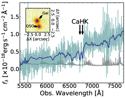
Figure 13: Spectrum of the foreground galaxy located 1$\farcs$57 North North–East of the optical position of the quasar P323$+$12 (light blue). The elliptical galaxy template from Mannucci et al. (2001) redshifted to $z_{\rm gal}=0.711$ and rescaled to the flux observed in the Pan-STARRS $i$–band $i_{\rm PS1,\,gal}=23.29$ mag is shown as a dark blue line (see subsection 5.7 for details). The inset plots the location of the galaxy with respect to the quasar in the pseudo–broad–band image obtained by collapsing the MUSE cube between 8200Å and 9200Å.

6 SUMMARY AND CONCLUSIONS

We conducted a sensitive search for extended Ly$\alpha$ emission around a sample of 31 $5.7<z<6.6$ quasars spanning absolute magnitudes from ${\rm M}_{\rm 1450}=-22.5$ mag to ${\rm M}_{\rm 1450}=-29.1$ mag. This ongoing VLT/MUSE effort represents the first statistical study of the circum–galactic medium of quasars during the epoch of reionization (see Figure 14). After subtracting the contribution of the central AGN, we unveil the presence of significant extended Ly$\alpha$ emission around 12 targets. The detected nebulosities extend out to $\sim 30$ kpc from the quasars and show a variety of morphologies and physical properties. The study of these systems reveals that:

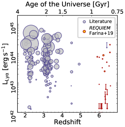
Figure 14: Redshift vs. total luminosity of all extended Ly$\alpha$ nebulae associated with QSOs known to date. Gray and orange points are data from the literature and from the REQUIEM survey, respectively. The size of the point is proportional to the area (in pkpc²) covered by each halo. Downward arrows are 3–$\sigma$ upper limits estimated integrating the nominal surface brightness limits over circular apertures with radius 20 pkpc. All values are uniformed to the concordance cosmology used in this paper (see Table 5 in Appendix E). However, effects of different sensitivities and observing technique are not taken into account.

1. The redshift of the extended emission well aligns with the systemic redshift of the quasar host–galaxies traced by the [C ii] 158 $\mu$m line with an average shift of $\langle\Delta V_{\rm sys}\rangle=(69\pm 36)$ km s^-1.

2. The luminosities of the halos appear to be independent of the amount of star formation in the host galaxy and of the UV luminosity of the central AGN.

3. The velocity dispersion of the gas in the halos is consistent with gravitational motion in dark matter halos of $M_{\rm DM}\lesssim 10^{13}$ M_⊙ at $z\sim 6$.

4. For most of our objects, we do not find clear evidence of rotation or ordered motion. However, the extended emission around the quasar P231$+$20 shows indications of a rotational pattern.

5. The surface brightness of the detected halos is consistent with the emission expected from optically thin clouds illuminated by the quasars. However, this requires high volume densities of the order $n_{\rm H}\gtrsim 1$ cm^-3.

6. The average surface brightness profile of the halos is well fit by an exponential curve. After correcting for redshift dimming and scaling distances by the virial radius of a halo of $10^{12.5}$ M_⊙, we observe no strong evolution of the profile between $z\sim 6$ and $z\sim 3$, followed by a decline in surface brightness down to $z\sim 2$.

7. The two quasars that have peculiarly small near zones ($R^{\rm corr}_{\rm p}\lesssim 3$ pMpc) do not show evidence for extended emission. This is consistent with a scenario where these quasars that have been shining for less than $\sim 10^{5}$ yr.

We can ask ourselves if the reservoirs of cool gas observed around the first quasars are sufficient to sustain the enormous star formation rates of the host galaxies (with depletion time of $t_{\rm dep}\sim 10-100$ Myr) and fast growth of the central supermassive black holes. The little evolution in the characteristics of the extended Ly$\alpha$ halos observed between $z\sim 6$ and $z\sim 3$ suggests that the emitting clouds retain similar properties within this redshift range. In this idealized model and assuming a spherical distribution for the clouds, the total mass in cool gas can be calculated as:

$$M_{\rm cool}=\pi Rf_{c}N_{\rm H}\frac{m_{p}}{X}.$$ (12)

Given that the extended emissions occur on scales of $10-30$ pkpc, we can roughly estimate $M_{\rm cool}\gtrsim 10^{9}$ M_⊙ around the first quasars. In general, hydrodynamical cosmological simulation are necessary to follow the complex journey of this gas from the IGM down to the host galaxy. However, given the observed kinematics, we can assume that the angular momentum has little impact in the accretion process and consider the free–fall time ($t_{\rm ff}=\sqrt{3\pi/32\,G\,\rho}\sim 50$ Myr) as the minimum time–scale over which gas inflows. This implies that, potentially, the rate of gas supply (of the order of ${\dot{M}}_{\rm cool}\sim 10-100$ M_⊙ yr^-1) is compatible with the SFR estimated for the quasar host galaxies. Further investigations of the detected nebulae are necessary to fully capture the physical status of the emitting material, however our REQUIEM survey suggest that the halos of the first quasars contain sufficient fuel to maintain the observed high–rate of gas consumption.

As the first IFS study aimed at mapping the Ly$\alpha$ emission around a statistical sample of $z>6$ quasars, the REQUIEM survey demonstrates that direct detection of the CGM of the first massive galaxies is possible in 1–10 hours of VLT/MUSE per target. The detected nebulae are unique targets for future multi–band follow–up observations to characterize the distribution of the gas and to constrain its physical conditions. In the near future, we will exploit the rich dataset provided by the REQUIEM survey to study the clustering of galaxies around these quasars (Paper II), to search for UV–bright counterparts of high–$z$ absorption selected galaxies (Paper III), and to perform a detailed comparison between the dynamics of the host–galaxies and the properties of the extended emission (Paper IV).

Appendix A Atlas of the quasars part of the REQUIEM survey

In Figure 15 we show the RGB postage stamps of the quasar vicinity created by combining three 2000 km s^-1 wide pseudo–narrow–band images: one located 16000 km s^-1 blueward, one 5000 km s^-1 redward, and one at the redshifted Ly$\alpha$ wavelength. The spectra of the quasars extracted over apertures with a radius two times larger than the seeing are also shown.

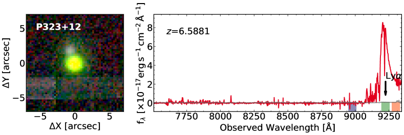
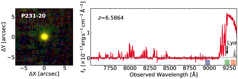
Figure 15: RGB images (left) and spectra (right) of the high–redshift quasars targeted in the REQUIEM survey (ordered by decreasing redshift). The wavelength ranges used to create the RGB images are highlighted with red, green, and blue boxes in the right panels. The wavelength of the Ly$\alpha$ line redshifted at $z_{\rm sys}$ is marked with a black arrow.

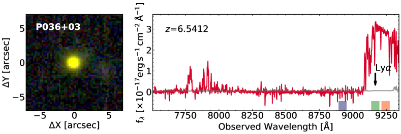
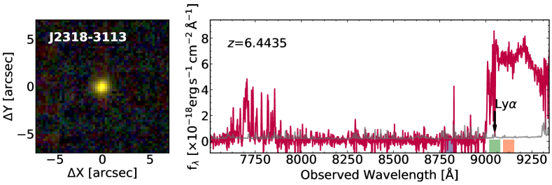
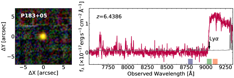
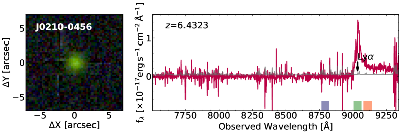
Figure 15: continued.

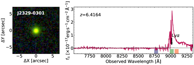
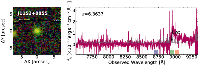
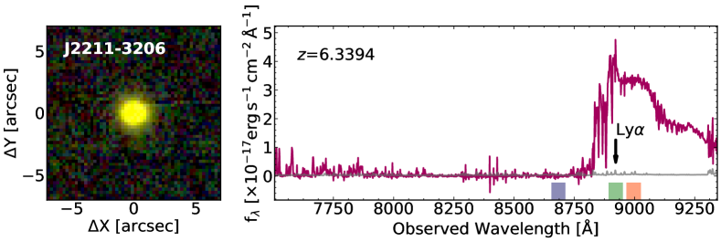
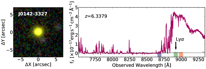
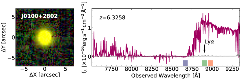
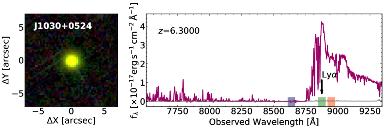
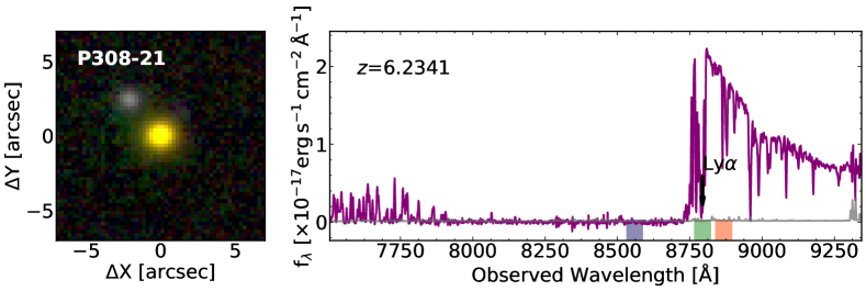
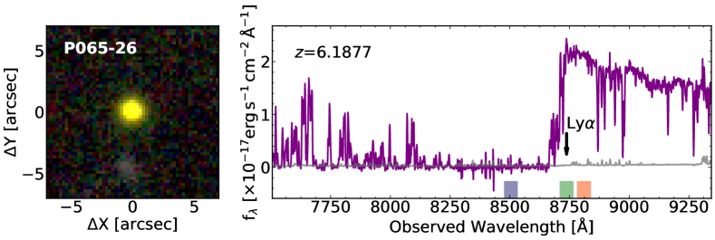
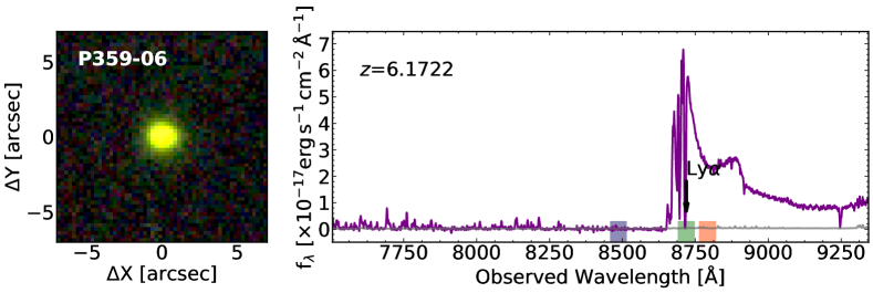
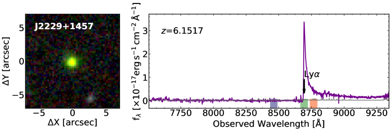
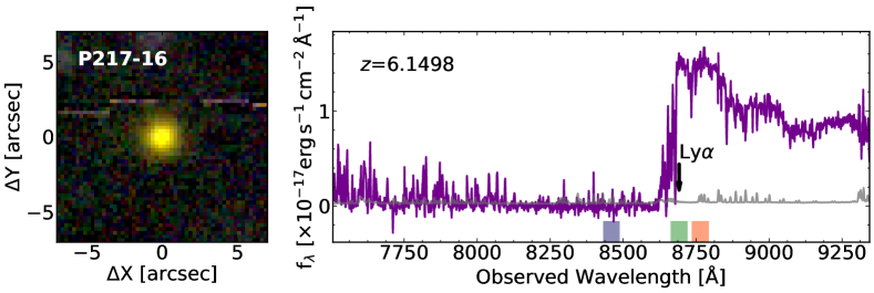
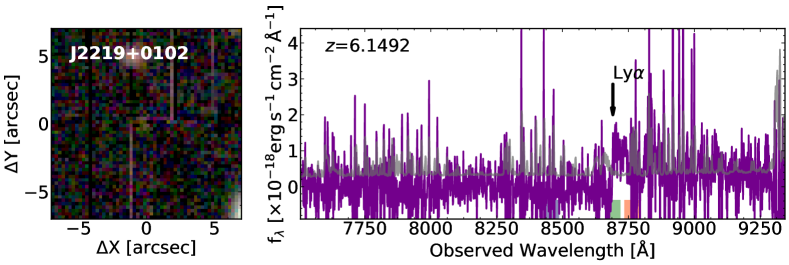
Figure 15: continued.

Figure 15: continued.

Figure 15: continued.

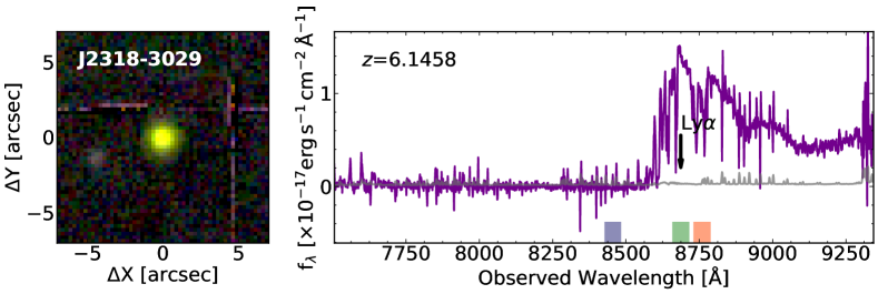
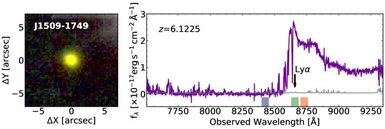
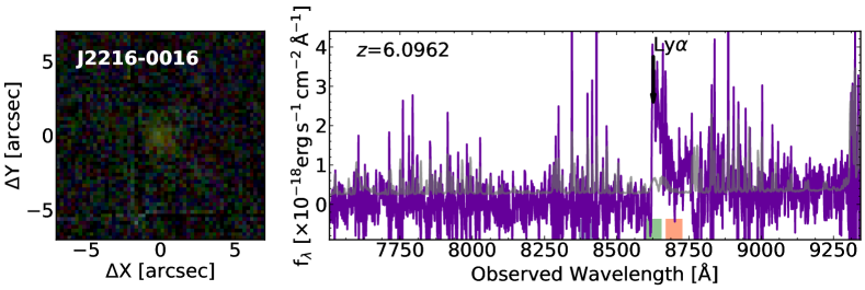
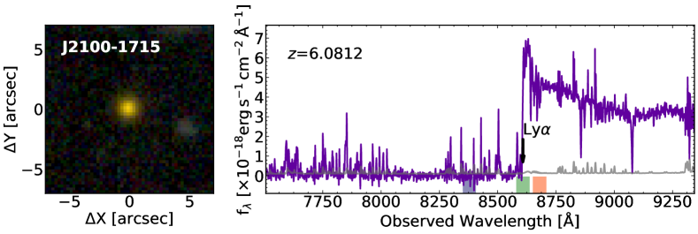
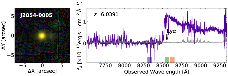
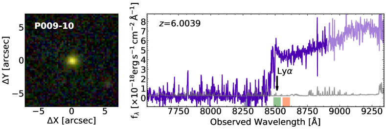
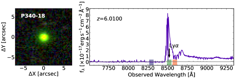
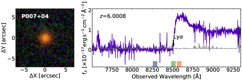
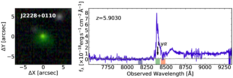
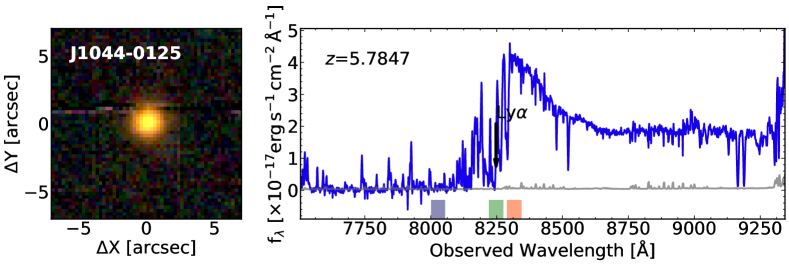
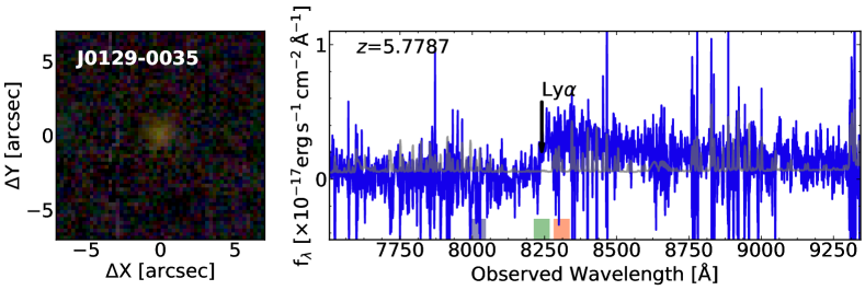
Figure 15: continued.

Figure 15: continued.

Figure 15: continued.

Appendix B The spectrum of P009$-$10

The spectrum of P009$-$10 plotted in Figure 15 shows a deviation from the typical blue slope of quasars at $\lambda>8700$ Å. This behavior appears to be independent from the spectrophotometric star used for flux calibration and from the frames used to correct for flat field. We argue that this is most probably due to imperfect illumination correction due to the rapid variation of the sky conditions occurred during the observation of the target during the night of August 3rd, 2018. This is supported by the strong variation on the background in the red side of different MUSE IFUs. However, given that the Ly$\alpha$ line is redshifted at $\lambda\sim 8500$ Å, this has no impact on the current analysis.

Appendix C Analysis of the LBT/LUCI2 + ARGOS images of P323$+$12

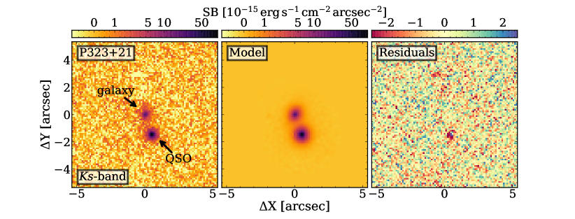
Figure 16: Results from the modelling of the quasar and close–by galaxy on the $Ks$–band images obtained with LBT/LUCI 2$+$ARGOS. Different panels show, from left to right: zoom–in on the 10″$\times$10″region centered on the galaxy; model of the quasar and galaxy emission; residuals after model subtraction (see Appendix C for details). In all panels, North is up and West is right.

High–resolution $Ks$–band images of the quasar P323$+$12 have been collected with the Large Binocular Telescope (LBT, Hill & Salinari, 2004; Hill et al., 2012) high with the Advanced Rayleigh guided Ground layer adaptive Optics System (ARGOS; Rabien et al., 2010, 2019) coupled with LUCI 2 (i.e., LBT Utility Camera in the Infrared; Seifert et al., 2003; Ageorges et al., 2010). Data where collected on 25^th October 2017 during an ARGOS commissioning run. The total time on targets was 660 s, divided in 263 individual 2.51 s exposures. The data reduction has been performed with standard IRAF routines following the procedure described in Farina et al. (2018) and Georgiev et al. (2019). We registered the image to the WCS using the Astrometry.net software (Lang et al., 2010). The absolute flux calibration was achieved by matching sources with the 2MASS catalogue (Cutri et al., 2003) and considering a Vega to AB conversion in the $K_{s}$–band of ${\rm m}_{\rm AB}-{\rm m}_{\rm Vega}=1.85$ mag. Uncertainty in the zeropoint is of the order of 0.1 mag. During the observations, the DIMM seeing was 1$\farcs$34 in the optical. The three green light (532 nm) lasers focused at 12 km used by ARGOS to correct for the ground layer turbulence, allowed us to enhance the $Ks$–band image quality to 0$\farcs$27 (FWHM of an unresolved source) of the entire LUCI 2 field–of–view. The 5–$\sigma$ detection limit for a point source (estimated from the rms of the sky counts integrated over the radius of an unresolved source) is $Ks_{\rm lim}=23.9$ mag.

We exploit this data to look for the possible presence of multiple lensed images of the quasar generated by the presence of the $z=0.711$ elliptical galaxy located 1$\farcs$6 NNE from the quasar (see subsection 5.7). First, we construct a spatially variable PSF model and we evaluated it at the quasar location (for further details see Farina et al., 2018; Georgiev et al., 2019). Then, we use this model to subtract both the emission from both the quasar and the close–by galaxy using the GALFIT v3.0.5 package (Peng et al., 2010, 2011 , see Figure 16). The galaxy emission is well represented by a Sérsic profile (Sérsic, 1963) with magnitude $Ks_{\rm gal}=(20.26\pm 0.16)$ mag, effective radius $R_{e}=(1.1\pm 0.3)$ arcsec, and Sérsic index $n=(4.9\pm 2.1)$. The quasar is unresolved, with apparent magnitude $Ks_{\rm QSO}=(19.33\pm 0.11)$ mag (see Figure 16). This implies that the host–galaxy is either compact (with radius $<1.5$ pkpc) or its emission is below a surface brightness of $\mu_{Ks,{\rm host}}>22.7$ mag arcsec^-1 5–$\sigma$ limit over a 1 arcsec² aperture). These limits are slightly looser, but consistent with those obtained by Mechtley et al. (2012) on the host galaxy of the $z=6.42$ quasar J1148$+$5251.

In the residual image we do not detect any source in the close proximity of the galaxy (down to a 2–$\sigma$ surface brightness limit of $\mu_{Ks,{\rm lim}}>23.7$ mag arcsec^-1 over an aperture of 1 arcsec²) that could be interpreted as multiple images of the quasar. This supports our simple model presented in subsection 5.7 where we showed that the Einstein ring is expected to be smaller than the separation between the quasar and the galaxy (i.e., $<1\farcs 6$).

Appendix D The median surface–brightness profile

In Figure 17 we show the surface brightness profile computed by median combining the profiles extracted from the pseudo–narrow band images of quasars part of the core sample of our REQUIEM survey (see subsection 4.2). Given the relatively small number of $z>5.5$ quasars observed with MUSE, we are not able to estimate the incidence of outliners (such as the nabulae with sizes $\gg 100$ pkpc observed around $\sim 1\%$ of intermediate redshift quasars, e.g., Hennawi et al., 2015; Arrigoni Battaia et al., 2019a) in our sample. We thus consider the average surface brightness profile presented in subsection 5.5 to be a more befitting depiction of the diffuse Ly$\alpha$ emission around $z\sim 6$ quasars. We notice, however, that our results do not depend on the type of profile chosen. A fit with the exponential function $(1+z)^{4}\,{\rm SB}_{\rm Ly\alpha}\left(r\right)=C\exp{\left(-r/r_{h}\right)}$ shows that the median profile has a slightly fainter normalization [$C=(2.2\pm 0.3)\times 10^{-14}$ erg s^-1 cm^-2 arcsec^-2] and a similar scale length [$r_{h}=(8.9\pm 0.6)$ kpc] with respect to the average profile (see subsection 5.5 and Figure 17).

Measured average and median surface brightness radial profiles of the extended Ly$\alpha$ emission around $z\sim 6$ quasars are tabulated in Table 4.

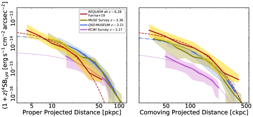
Figure 17: Left Panel – Median Ly$\alpha$ surface brightness profiles around quasars at different redshifts. Measurements are from the core sample of our REQUIEM survey (dark orange line), Marino et al. (2019 , olive green line), Arrigoni Battaia et al. (2019a , light blue line), and Cai et al. (2019 , magenta line). All data are corrected for cosmological dimming. Shaded regions represents the 25th–75th percentiles in each quasar sample. Exponential best fits are shown in the same color palette. Right Panel – Same of Left Panel, but in comoving units.

Table 4: Average and median Ly$\alpha$ surface brightness profile around quasars in the core sample of the REQUIEM survey

Radius	average Ly$\alpha$ SB	RMS	median Ly$\alpha$ SB	25th percentile	75th percentile
(pkpc)	($10^{-16}$ erg s-1 cm-2 arcsec-2)
string4.2	259.2	232.7	198.7	101.3	345.7
string6.5	162.7	128.2	120.8	string77.9	175.5
string9.9	string88.1	string67.9	string60.5	string37.6	106.7
15.3	string57.7	string53.7	string39.2	string28.0	string65.5
23.4	string23.9	string22.8	string18.5	string8.8	string25.3
35.9	string7.6	string8.7	string4.0	string2.1	string9.6
55.0	string2.2	string1.4	string2.1	string1.6	string3.4

Note. — All measurements are corrected for cosmological surface brightness dimming.

Appendix E List of known Ly$\alpha$ nebulae associated to quasars

Table 5 lists sizes and luminosities of the extended Ly$\alpha$ nebulae associated to quasars known as of the end of October 2019. Data are homogenized to the cosmology used in this paper. However, no attempt has been made to correct for the different sensitivities or for the diverse observing techniques employed in the listed studies.

Table 5: Ly$\alpha$ nebulae associated to quasars from the literature.

ID	Type	$z$	dLyα	LLyα	Ref.
			(pkpc)	($10^{43}$ erg s-1)
Q1658$+$575	QSO–RL	1.979	string89string	string9.9string	Heckman et al. (1991b)
Q0017$+$154	QSO–RL	2.012	string97string	12.9string	Heckman et al. (1991b)
Q1354$+$258	QSO–RL	2.032	string88string	21.1string	Heckman et al. (1991b)
Q0225$-$014	QSO–RL	2.037	string44string	string5.3string	Heckman et al. (1991b)
Q1345$+$258	QSO–RL	2.039	string79string	26.8string	Heckman et al. (1991b)
Jackpot	4$\times$QSO	2.040	310string	21.0string	Hennawi et al. (2015)
Q0445$+$097	QSO–RL	2.113	106string	string7.3string	Heckman et al. (1991a, b)
J0112$-$0048	QSO	2.149	string42string	string3.0string	Fathivavsari et al. (2016)
Q0109$+$176	QSO–RL	2.157	string26string	string1.5string	Heckman et al. (1991b)
Q1318$+$113	QSO–RL	2.176	string96string	25.0string	Heckman et al. (1991a, b)
J1154$-$0215	QSO	2.181	string50string	string2.4string	Fathivavsari et al. (2016)
Q2125$+$0112	QSO	2.203	string19string	string1.3string	Cai et al. (2019)
Q0050$+$0051	QSO	2.222	116string	string2.0string	Cai et al. (2019)
Q0814$+$3250	QSO	2.222	string85string	string0.2string	Cai et al. (2019)
Q1228$+$3128	QSO	2.231	124string	12.3string	Cai et al. (2019)
J2233$-$606	QSO	2.238	105string	13.6string	Bergeron et al. (1999)
Q1444$+$3904	QSO	2.250	101string	10.1string	Cai et al. (2019)
Q1426$+$2555	QSO	2.256	string96string	string3.9string	Cai et al. (2019)
Q2127$+$0049	QSO	2.261	string58string	string1.1string	Cai et al. (2019)
Q0107$+$0314	QSO	2.262	114string	string1.5string	Cai et al. (2019)
Q1227$+$2848	QSO	2.268	164string	string5.8string	Cai et al. (2019)
Q2123$-$0050	QSO	2.271	154string	string3.6string	Cai et al. (2019)
Slug	2$\times$QSO	2.279	460string	22.0string	Cantalupo et al. (2014); Martin et al. (2015, 2019)
Q0052$+$0140	QSO	2.300	127string	string2.0string	Cai et al. (2019)
Q1416$+$2649	QSO	2.301	141string	string5.0string	Cai et al. (2019)
J1058$+$0315	QSO	2.302	string34string	string1.6string	Fathivavsari et al. (2016)
Q0848$-$0114	QSO	2.302	string28string	string0.1string	Cai et al. (2019)
MAMMOTH-1	QSO	2.311	442string	51.0string	Cai et al. (2017)
Q1230$+$3320	QSO	2.313	204string	12.4string	Cai et al. (2019)
Q2150$+$053	QSO–RL	2.323	string87string	string7.4string	Heckman et al. (1991b)
Q0048$+$0056	QSO	2.327	104string	string2.3string	Cai et al. (2019)
Q2222$+$051	QSO–RL	2.328	104string	string7.4string	Heckman et al. (1991b)
NDFWS J143725$+$351048	QSO	2.332	string80	string5.3string	Yang et al. (2009)
Q2121$+$0052	QSO	2.377	141string	string4.6string	Cai et al. (2019)
ELAN0101$+$020	2$\times$QSO	2.450	232string	45.0string	Cai et al. (2018)
J0049$+$3510	QSO	2.480	string85string	35.4string	Barrio et al. (2008)
TXS 1436$+$157	QSO–RL	2.537	string92string	string4.6string	Roettgering et al. (1997); van Ojik et al. (1997); Humphrey et al. (2013)
Q2206$-$199	QSO	2.577	string80string	$\cdots$	Møller et al. (2000)
J0953$+$0349	QSO	2.594	string29string	string1.3string	Fathivavsari et al. (2016)
Q2338$+$042	QSO–RL	2.594	string94string	15.4string	Heckman et al. (1991b); Lehnert & Becker (1998)
Q0758$+$097	QSO–RL	2.683	110string	10.5string	Heckman et al. (1991a, b)
Q0730$+$257	QSO–RL	2.686	string93string	string5.3string	Heckman et al. (1991b)
AMS05	QSO	2.850	string66string	string2.7string	Smith et al. (2009)
Q0805$+$046	QSO–RL	2.877	116string	62.8string	Heckman et al. (1991a, b)
Q0941$+$261	QSO–RL	2.913	string99string	string6.4string	Heckman et al. (1991a, b)
J1253$+$1007	QSO	3.015	string49string	string8.5string	Fathivavsari et al. (2016)
CTS A31.05	QSO	3.020	120string	string6.1string	Borisova et al. (2016)
J1135$-$0221	2$\times$QSO	3.020	string60string	32.0string	Arrigoni Battaia et al. (2019b)
UM669	QSO	3.021	160string	10.0string	Borisova et al. (2016)
J0952$+$0114	QSO	3.020	string58	58.3string	Marino et al. (2019)
Q0041$-$2638	QSO	3.036	170string	string2.9string	Borisova et al. (2016)
SDSSJ0219$-$0215	QSO	3.036	string87	string3.5string	Arrigoni Battaia et al. (2019a)
Q1205$-$30	QSO	3.047	string81	string5.8string	Arrigoni Battaia et al. (2019a)
Q1759$+$7539	QSO	3.049	string65string	string9.0string	Christensen et al. (2006)
Q1205$-$30	QSO	3.040	string40string	string6.3string	Weidinger et al. (2004, 2005); Fynbo et al. (2000)
HE0940$-$1050	QSO	3.050	170string	14.0string	Borisova et al. (2016)
SDSSJ1342$+$1702	QSO	3.053	100	string2.4string	Arrigoni Battaia et al. (2019a)
SDSSJ0947$+$1421	QSO	3.073	string80	string2.0string	Arrigoni Battaia et al. (2019a)
LBQS1209$+$1524	QSO	3.075	108	string3.2string	Arrigoni Battaia et al. (2019a)
AWL 11	QSO	3.079	130string	string4.9string	Borisova et al. (2016)
SDSSJ0100$+$2105	QSO	3.097	string67	string5.0string	Arrigoni Battaia et al. (2019a)
TEX1033$+$137	QSO–RL	3.097	122	12.7string	Arrigoni Battaia et al. (2019a)
Q-N1097.1	QSO	3.099	string87	string3.0string	Arrigoni Battaia et al. (2019a)
Q0058$-$292	QSO	3.101	109	string3.8string	Arrigoni Battaia et al. (2019a)
S3 1013$+$20	QSO–RL	3.108	110	string5.6string	Arrigoni Battaia et al. (2019a)
SDSSJ1240$+$1455	QSO	3.113	string40string	string4.2string	Matsuda et al. (2011)
CTS A11.09	QSO	3.121	150string	string2.1string	Borisova et al. (2016)
J0525$-$233	QSO–RL	3.123	string77	string1.2string	Arrigoni Battaia et al. (2019a)
CT 656	QSO	3.125	130string	string2.8string	Borisova et al. (2016)
SDSSJ1209$+$1138	QSO	3.126	string83	string2.3string	Arrigoni Battaia et al. (2019a)
CTSH22.05	QSO	3.127	123	string7.4string	Arrigoni Battaia et al. (2019a)
UM672	QSO–RL	3.127	string93	string6.5string	Arrigoni Battaia et al. (2019a)
CTS B27.07	QSO	3.132	160string	10.0string	Borisova et al. (2016)
Q0140$-$306	QSO–RL	3.132	113	string5.1string	Arrigoni Battaia et al. (2019a)
UM683	QSO	3.132	142	string7.9string	Arrigoni Battaia et al. (2019a)
SDSSJ2100$-$0641	QSO	3.136	string68	string2.1string	Arrigoni Battaia et al. (2019a)
SDSSJ0814$+$1950	QSO–RL	3.137	string50	string2.6string	Arrigoni Battaia et al. (2019a)
SDSSJ0827$+$0300	QSO–RL	3.137	string57	string0.8string	Arrigoni Battaia et al. (2019a)
PKS0537$-$286	QSO–RL	3.141	112	string4.6string	Arrigoni Battaia et al. (2019a)
Q2138$-$4427	QSO	3.142	string82	string4.7string	Arrigoni Battaia et al. (2019a)
SDSSJ1550$+$0537	QSO	3.147	string99	string5.6string	Arrigoni Battaia et al. (2019a)
LBQS1244$+$1129	QSO	3.157	101	string5.2string	Arrigoni Battaia et al. (2019a)
6dF J0032$-$0414	QSO–RL	3.162	149	35.7string	Arrigoni Battaia et al. (2019a)
UM24	QSO	3.163	107	string2.6string	Arrigoni Battaia et al. (2019a)
SDSSJ0905$+$0410	QSO–RL	3.165	string98	string2.8string	Arrigoni Battaia et al. (2019a)
PKS1017$+$109	QSO	3.167	185	24.9string	Arrigoni Battaia et al. (2019a)
SDSSJ1020$+$1040	3$\times$QSO	3.167	297string	32.2string	Arrigoni Battaia et al. (2018a)
SDSSJ2319$-$1040	QSO	3.172	string86	string3.2string	Arrigoni Battaia et al. (2019a)
SDSSJ1243$+$0720	QSO–RL	3.178	string89	string5.1string	Arrigoni Battaia et al. (2019a)
Q2204$-$408	QSO	3.179	string30	string1.1string	Arrigoni Battaia et al. (2019a)
J0823$+$0529	QSO	3.188	string45string	16.8string	Fathivavsari et al. (2016)
UM678	QSO	3.188	150string	string7.8string	Borisova et al. (2016)
SDSSJ2348$-$1041	QSO	3.190	string92	string2.3string	Arrigoni Battaia et al. (2019a)
SDSSJ1032$+$1206	QSO–RL	3.195	string58	string1.5string	Arrigoni Battaia et al. (2019a)
Q0052$-$3901A	QSO–RL	3.203	120	string9.8string	Arrigoni Battaia et al. (2019a)
UM670	QSO	3.203	string92	string2.8string	Arrigoni Battaia et al. (2019a)
Q1425$+$606	QSO	3.204	string37string	10.1string	Christensen et al. (2006)
SDSSJ0819$+$0823	QSO	3.205	158	38.7string	Arrigoni Battaia et al. (2019a)
CTS G18.01	QSO	3.207	240string	17.0string	Borisova et al. (2016)
PKS1614$+$051	QSO	3.215	string50string	string2.0string	Husband et al. (2015)
UM679	QSO	3.215	string94	string4.5string	Arrigoni Battaia et al. (2019a)
PKS1614$+$051	QSO–RL	3.217	string66string	string7.3string	Hu, & Cowie (1987)
CT-669	QSO	3.218	string97	11.0string	Arrigoni Battaia et al. (2019a)
PKS1614$+$051	QSO	3.210	string40string	10.3string	Matsuda et al. (2011)
Q0115$-$30	QSO	3.221	string46	string0.3string	Arrigoni Battaia et al. (2019a)
Q2139$-$4434	QSO	3.221	140	string6.8string	Arrigoni Battaia et al. (2019a); Lusso et al. (2019)
Q2139$-$4433	QSO	3.229	100	string2.5string	Lusso et al. (2019)
SDSSJ1307$+$1230	QSO	3.229	117	string7.0string	Arrigoni Battaia et al. (2019a)
Q0347$-$383	QSO	3.230	113	string4.1string	Arrigoni Battaia et al. (2019a)
SDSSJ2321$+$1558	QSO	3.241	string71	string0.9string	Arrigoni Battaia et al. (2019a)
SDSSJ1025$+$0452	QSO	3.243	144	18.7string	Arrigoni Battaia et al. (2019a)
CTS C22.31	QSO	3.246	101	string5.0string	Arrigoni Battaia et al. (2019a)
Q0057$-$3948	QSO	3.251	107	string5.1string	Arrigoni Battaia et al. (2019a)
Q1451$+$122	QSO	3.253	string16string	string1.9string	Christensen et al. (2006)
Q0042$-$2627	QSO	3.280	320string	17.0string	Borisova et al. (2016)
SDSSJ1557$+$1540	QSO	3.288	107	21.8string	Arrigoni Battaia et al. (2019a)
Q2233$+$131	QSO	3.301	string11string	string1.2string	Christensen et al. (2006)
Q0956$+$122	QSO	3.309	string90string	string5.6string	Fumagalli et al. (2016)
Q0956$+$1217	QSO	3.316	106	string5.3string	Arrigoni Battaia et al. (2019a)
SDSSJ0125$-$1027	QSO	3.319	string43	string2.3string	Arrigoni Battaia et al. (2019a)
Q2348$-$4025	QSO	3.334	103	string5.1string	Arrigoni Battaia et al. (2019a)
SDSSJ0250$-$0757	QSO	3.336	string86	string2.9string	Arrigoni Battaia et al. (2019a)
SDSSJ0817$+$1053	QSO	3.336	102	string5.0string	Arrigoni Battaia et al. (2019a)
SDSSJ0154$-$0730	QSO	3.337	string83	string3.3string	Arrigoni Battaia et al. (2019a)
SDSSJ1337$+$0218	QSO	3.344	string51	string0.5string	Arrigoni Battaia et al. (2019a)
SDSSJ0001$-$0956	QSO–RL	3.348	131	10.8string	Arrigoni Battaia et al. (2019a)
CTS R07.04	QSO	3.351	170string	33.0string	Borisova et al. (2016)
SDSSJ1427$-$0029	QSO	3.354	string49	string4.1string	Arrigoni Battaia et al. (2019a)
Q0042$-$269	QSO	3.357	string61	string1.0string	Arrigoni Battaia et al. (2019a)
FBQSJ2334$-$0908	QSO–RL	3.361	string52	string0.7string	Arrigoni Battaia et al. (2019a)
Q2355p0108	QSO	3.395	121	string5.4string	Arrigoni Battaia et al. (2019a)
SDSSJ1019$+$0254	QSO	3.395	string73	string3.1string	Arrigoni Battaia et al. (2019a)
SDSSJ1429$-$0145	QSO	3.425	string79	string3.6string	Arrigoni Battaia et al. (2019a)
SDSSJ1057$-$0139	QSO–RL	3.452	string65	string1.7string	Arrigoni Battaia et al. (2019a)
0054$-$284	QSO	3.616	string38string	string0.8string	Bremer et al. (1992)
Q0055$-$269	QSO	3.634	180string	37.0string	Borisova et al. (2016)
0055$-$264	QSO	3.656	string30string	1.1 string	Bremer et al. (1992)
Q1621$-$0042	QSO	3.689	120string	string5.5string	Borisova et al. (2016)
Q1317$-$0507	QSO	3.701	140string	string3.6string	Borisova et al. (2016)
QB2000$-$330	QSO–RL	3.759	120string	12.0string	Borisova et al. (2016)
PKS1937$-$101	QSO–RL	3.769	110string	29.0string	Borisova et al. (2016)
J0124$+$0044	QSO	3.783	190string	41.0string	Borisova et al. (2016)
BRI1108$-$07	QSO	3.907	160string	12.0string	Borisova et al. (2016)
Q0953$+$4749	QSO	4.489	string14string	string0.8string	Christensen et al. (2006); Bunker et al. (2003)
BR1033$-$0327	QSO	4.510	string70string	string2.4string	North et al. (2012); Courbin et al. (2008)
SDSSJ14472$+$0401	QSO	4.510	string42string	string0.2string	North et al. (2012)
SDSSJ21474$-$0838	QSO	4.510	string56string	23.2string	North et al. (2012)
1605$-$0112	QSO	4.920	string60string	string4.4string	Ginolfi et al. (2018)
J2228$+$0110	QSO–RL	5.903	string30string	string7.8string	Roche et al. (2014); Drake et al. (2019); Farina et al. (2019)
P009$-$10	QSO	6.004	string15string	string0.9string	Farina et al. (2019)
P340$-$18	QSO	6.010	string18string	string7.5string	Farina et al. (2019)
P359$-$06	QSO	6.172	string17string	string3.3string	Farina et al. (2019)
P065$-$26	QSO	6.188	string25string	string6.6string	Farina et al. (2019)
P308$-$21	QSO	6.234	string43string	string8.8string	Farina et al. (2019)
J1030$+$0524	QSO	6.300	string34string	string2.5string	Decarli et al. (2012); Drake et al. (2019); Farina et al. (2019)
J2329$-$0301	QSO	6.416	string22string	string5.1string	Farina et al. (2019)
J2329$-$0301	QSO	6.416	string22string	string5.1string	Goto et al. (2009, 2012); Willott et al. (2011); Momose et al. (2019); Drake et al. (2019); Farina et al. (2019)
P036$+$03	QSO	6.541	string19string	string3.8string	Farina et al. (2019)
P231$-$20	QSO	6.586	string28string	11.0string	Drake et al. (2019); Farina et al. (2019)
P323$+$12	QSO	6.588	string25string	20.1string	Farina et al. (2019)
J0305$-$3150	QSO	6.615	string17string	string0.8string	Farina et al. (2017, 2019)

Note. — The ‘Type’ indicates if the nebula is associated with a radio–loud quasar (QSO–RL), a radio–quiet quasar (QSO), or with a system of multiple quasars ($N\times$QSO). The size is the maximum diameter distance of the Ly$\alpha$ emission. The table is published in its entirety in the machine-readable format. A portion is shown here for guidance regarding its form and content.

References

- (1)
- Ageorges et al. (2010) Ageorges, N., Seifert, W., Jütte, M., et al. 2010, Proc. SPIE, 7735, 77351L
- Alam & Miralda-Escudé (2002) Alam, S. M. K., & Miralda-Escudé, J. 2002, ApJ, 568, 576