Impact of Isolation and Fiducial Cuts on $q_{T}$ and N-Jettiness Subtractions

Abstract

Kinematic selection cuts and isolation requirements are a necessity in experimental measurements for identifying prompt leptons and photons that originate from the hard-interaction process of interest. We analyze how such cuts affect the application of the $q_{T}$ and $N$-jettiness subtraction methods for fixed-order calculations. We consider both fixed-cone and smooth-cone isolation methods. We find that kinematic selection and isolation cuts both induce parametrically enhanced power corrections with considerably slower convergence compared to the standard power corrections that are already present in inclusive cross sections without additional cuts. Using analytic arguments at next-to-leading order we derive their general scaling behavior as a function of the subtraction cutoff. We also study their numerical impact for the case of gluon-fusion Higgs production in the $H\to\gamma\gamma$ decay mode and for $pp\to\gamma\gamma$ direct diphoton production. We find that the relative enhancement of the additional cut-induced power corrections tends to be more severe for $q_{T}$, where it can reach an order of magnitude or more, depending on the choice of parameters and subtraction cutoffs. We discuss how all such cuts can be incorporated without causing additional power corrections by implementing the subtractions differentially rather than through a global slicing method. We also highlight the close relation of this formulation of the subtractions to the projection-to-Born method.

1 Introduction

An important class of measurements at colliders such as the LHC are processes involving leptons or photons in the final state. For example, the cleanest channels to measure Higgs production are the $H\to 4\ell$ and $H\to{\gamma\gamma}$ decay modes, and both have been studied extensively by ATLAS and CMS [1, 2, 3, 4, 5, 6, 7, 8]. Other important examples are inclusive $W\to\ell\nu$ and $Z/\gamma^{*}\to\ell\ell$ production [9, 10, 11, 12, 13, 14], direct diphoton production $pp\to{\gamma\gamma}$ [15, 16, 17, 18], and more generally any process involving prompt photons or electroweak bosons in leptonic decay channels. In all such measurements, lepton and photon kinematic selection cuts and isolation requirements are necessary to identify the leptons and photons originating from the hard interaction and to suppress backgrounds such as misidentified jets or secondary leptons and photons arising for example from the decay of hadrons.

The most prominent selection cuts are minimum $p_{T}$ requirements. The isolation is commonly achieved by restricting the energy in a cone around the lepton or photon to be bounded, for example

$$\sum_{i:\,d(i,\gamma/\ell)<R}E_{T}^{i}<E_{T}^{\rm iso}\,,$$ (1.1)

where the sum runs over all particles $i$ in a cone of size $R$ around the photon $\gamma$ or lepton $\ell$.

Since isolation requirements as in eq. (1.1) are sensitive to the momenta of all hadrons in an event, incorporating them into higher-order calculations requires one to explicitly take into account the isolation cuts when integrating over the phase space of real emissions. This in turn requires fixed-order calculations that are fully exclusive in the final state of real emissions. A key challenge in higher-order calculations is the cancellation of infrared (IR) divergences from the soft and collinear limits of real emissions against corresponding divergences from virtual corrections. At NLO, fully-exclusive calculations are achieved by applying local subtraction techniques such as the FKS [19, 20] or CS [21, 22, 23] subtractions. At next-to-next-to-leading order (NNLO), local subtraction techniques become much more involved due to the overlap of virtual and real divergences, and a variety of such methods have been developed [24, 25, 26, 27, 28, 29, 30, 31, 32, 33, 34, 35, 36].

Another approach to obtain fully-exclusive NNLO calculations is the use of global slicing methods [37, 38, 39], where one exploits that the cancellation of IR divergences occurs in the singular limit of a suitable resolution variable, and that this singular limit can be predicted from a factorization theorem. For the transverse momentum $q_{T}$, the relevant factorization was first shown in refs. [40, 41, 42]. For $N$-jettiness ${\mathcal{T}}_{N}$ [43], the relevant factorization was derived in refs. [44, 43] using the soft-collinear effective theory (SCET) [45, 46, 47, 48, 49]. All contributions to the cross section not described by the factorization, usually referred to as nonsingular terms or power corrections, can then be obtained from an NLO calculation. Hence, an advantage of the slicing methods is that they are comparably straightforward to implement, since they allow reusing much of the existing NLO calculations. For the same reasons, they are also extendable to N³LO [39, 50, 51].

An important aspect of slicing methods is that they require a resolution cutoff, which induces power corrections from contributions below the cutoff that are neglected. To improve the numerical performance, these power corrections can be included systematically by computing them in an expansion in the resolution variable about the soft and collinear limits. Recently, there has been significant interest and progress in understanding collider cross sections at subleading power [52, 53, 54, 55, 56, 57, 58, 59, 60, 61, 62, 63, 64, 65, 66, 67, 68, 69]. In particular, for inclusive Higgs and Drell-Yan production the leading-logarithmic (LL) corrections at NNLO at next-to-leading power (NLP) are known for ${\mathcal{T}}_{0}$ [70, 71, 72]. At NLO, the full NLP corrections are known for ${\mathcal{T}}_{0}$ [73, 74], $q_{T}$ [75], and ${\mathcal{T}}_{1}$ [76].

The same power corrections are also important for the resummation of logarithms $\ln(q_{T}/Q)$ or $\ln({\mathcal{T}}_{0}/Q)$ in the $q_{T}$ or ${\mathcal{T}}_{0}$ spectra at small $q_{T}\ll Q$ or ${\mathcal{T}}_{0}\ll Q$ (with $Q$ being the relevant hard-interaction scale). This resummation is based on the same factorization theorems underlying the subtraction methods, as the logarithmic terms precisely arise in the singular limit of the cross section. In addition to the resummed singular cross section, one has to include the power corrections in order to recover the full fixed-order result for the spectrum. Thus, understanding the effect of selection and isolation cuts on the factorization is equally important for resummation.

So far, studies of power corrections have only considered inclusive processes, while the effect of selection and isolation cuts have not yet been considered. As we will see, these cuts are an additional source of power corrections. Given their necessity for experimental measurements, it is important to study the cut-induced power corrections, and in particular determine if and when they lead to the dominant corrections or if they can even lead to a breakdown of the factorization and thus the subtraction methods.

In this paper, we study the effect of kinematic selection and isolation cuts on $q_{T}$ and ${\mathcal{T}}_{0}$ factorization. For concreteness, we focus on the case of diphoton production, either in the direct process $pp\to{\gamma\gamma}$ or the Higgs decay mode $pp\to H\to{\gamma\gamma}$. We will therefore primarily talk about photons, but we stress that our results and conclusions apply equally to leptons. Using a simplified calculation at NLO, we determine the scaling of power corrections induced by the cuts. In particular, we discuss the dependence on the isolation method and parameters, considering both fixed-cone and smooth-cone isolations. We will find that the cuts induce power corrections that are parametrically enhanced, and which can thus be significantly larger than for the case without cuts. This enhancement is particularly severe for the case of $q_{T}$ subtractions with smooth-cone isolation. This has important ramifications for the numerical stability of the subtractions in practical applications. In fact, in refs. [77, 78] it was already observed numerically that processes involving photon isolation suffer from large enhanced power corrections, which is explained by our results.

Given the potentially significant size of the cut-induced power corrections, it is essential to account for them. Since in general they are complicated and cut specific, including them by an explicit analytic calculation (e.g. along the lines of the inclusive ones discussed above) would be challenging and tedious. Differential subtractions [39] offer a way to avoid the power corrections because they do not require the finite cutoff that is necessary in the slicing approach. Exploiting this, we propose a strategy to incorporate the measurement cuts exactly such that the additional cut-induced power corrections are avoided. It uses the Born-like measurement that appears in the singular subtractions to separate the cut-induced power corrections from the inclusive, cut-independent ones, where the former can be kept exactly while the latter can be treated in the standard way. We also show that in this way the projection-to-Born method [31] naturally appears as the special case where the inclusive, cut-independent power corrections are fully known.

This paper is structured as follows. In section 2, we briefly review the $q_{T}$ and ${\mathcal{T}}_{N}$ subtraction formalism and give an overview of different photon isolation methods. We then provide a simple analytic study of the effect of both selection and isolation cuts on the subtraction techniques in section 3, before verifying our results numerically in section 4. Finally in section 5, we discuss how to incorporate the additional measurement cuts into the subtractions. We conclude in section 6.

2 Review of subtractions and photon isolation

2.1 Review of $q_{T}$ and ${\mathcal{T}}_{N}$ subtractions

In this section, we briefly review the $q_{T}$ and ${\mathcal{T}}_{N}$ subtraction methods. For a detailed discussion we refer to ref. [39].

We denote the relevant dimensionful resolution variable generically as ${\mathcal{T}}$ and its dimensionless version as $\tau$. For the case of color-singlet production ($N=0$), it can be chosen as the total transverse momentum of the color-singlet final state, ${\mathcal{T}}\equiv q_{T}^{2}$, which yields $q_{T}$ subtractions [37]. For $0$-jettiness subtractions, it is given by $0$-jettiness (aka beam thrust) ${\mathcal{T}}\equiv{\mathcal{T}}_{0}$. In terms of the hadronic final-state momenta $k_{i}$, these are defined as

$${\mathcal{T}} \equiv q_{T}^{2}=\Bigl{(}\sum_{i}\vec{k}_{T,i}\Bigr{)}^{2}\,,\qquad \tau\equiv q_{T}^{2}/Q^{2}\,,$$ (2.1)

$${\mathcal{T}} \equiv{\mathcal{T}}_{0}^{\mathrm{lep}}=\sum_{i}{\rm min}\bigl{\{}k_{i}^{+}e^{Y}\,,\,k_{i}^{-}e^{-Y}\bigr{\}}\,,\qquad \tau\equiv{\mathcal{T}}_{0}^{\rm lep}/Q\,.$$ (2.2)

Here, the sums over real emissions $i$ in the final state. The $k^{+}=n\cdot k$ and $k^{-}={\bar{n}}\cdot k$ are lightcone momenta, with $n^{\mu}=(1,0,0,1)$ and ${\bar{n}}^{\mu}=(1,0,0,-1)$ being lightlike reference vectors along the beam directions, and $Q$ and $Y$ are the total invariant mass and rapidity of the Born (the color-singlet) final state.

A key property of $\tau$ is that it is an IR-safe $N$-jet resolution variable, i.e. it vanishes for the Born process and in the IR-singular limit where all real emissions $k_{i}$ become soft or collinear. We can thus write the cross section $\sigma(X)$ as an integral over the cross section differential in $\tau$,

$$\sigma(X)=\int\!\mathrm{d}\tau\,\frac{\mathrm{d}\sigma(X)}{\mathrm{d}\tau}=\sigma(X,\tau_{\mathrm{cut}})+\int_{\tau_{\mathrm{cut}}}\!\mathrm{d}\tau\,\frac{\mathrm{d}\sigma(X)}{\mathrm{d}\tau}\,,$$ (2.3)

where the cumulative cross section as a function of $\tau_{\mathrm{cut}}$ is defined as

$$\sigma(X,\tau_{\mathrm{cut}})=\int^{\tau_{\mathrm{cut}}}\!\mathrm{d}\tau\,\frac{\mathrm{d}\sigma(X)}{\mathrm{d}\tau}\,.$$ (2.4)

Here, $X$ denotes all measurements. It includes the measurements performed on the Born process, including any selection cuts on its constituents. It also contains any additional cuts on the hadronic final state such as isolation cuts.

The slicing method is obtained by adding and subtracting a global subtraction term $\sigma^{\mathrm{sub}}(X,\tau_{\mathrm{cut}})$,

$$\sigma(X) =\sigma^{\mathrm{sub}}(X,\tau_{\mathrm{cut}})+\int_{\tau_{\mathrm{cut}}}\!\mathrm{d}\tau\,\frac{\mathrm{d}\sigma(X)}{\mathrm{d}\tau}+\Delta\sigma(X,\tau_{\mathrm{cut}})\,,$$

$$\Delta\sigma(X,\tau_{\mathrm{cut}}) =\sigma(X,\tau_{\mathrm{cut}})-\sigma^{\mathrm{sub}}(X,\tau_{\mathrm{cut}})\,.$$ (2.5)

Since $\tau$ vanishes by construction in the Born limit, the integral in eq. (2.1) necessarily involves at least one resolved real emission, and hence $\mathrm{d}\sigma(X)/\mathrm{d}\tau$ can be calculated from the corresponding Born+1-parton calculation at one lower order. The key requirement on $\sigma^{\mathrm{sub}}(X,\tau_{\mathrm{cut}})$ is that it must contain the leading terms in the $\tau_{\mathrm{cut}}\to 0$ limit. If that is the case, then $\Delta\sigma(X,\tau_{\mathrm{cut}})$ is a power correction of $\mathcal{O}(\tau_{\mathrm{cut}})$ which vanishes as $\tau_{\mathrm{cut}}\to 0$ and hence it can be neglected for sufficiently small $\tau_{\mathrm{cut}}$.

To construct $\sigma^{\mathrm{sub}}$ and study the size of $\Delta\sigma$, it is useful to expand the differential cross section and its cumulant for $\tau\ll 1$ and correspondingly $\tau_{\mathrm{cut}}\ll 1$,

$$\frac{\mathrm{d}\sigma(X)}{\mathrm{d}\tau} =\frac{\mathrm{d}\sigma^{(0)}(X)}{\mathrm{d}\tau} +\sum_{m>0}\frac{\mathrm{d}\sigma^{(2m)}(X)}{\mathrm{d}\tau}\,,$$ (2.6)

$$\sigma(X,\tau_{\mathrm{cut}}) =\sigma^{(0)}(X,\tau_{\mathrm{cut}}) +\sum_{m>0}\sigma^{(2m)}(X,\tau_{\mathrm{cut}})\,,$$

where the different contributions scale as

$$\frac{\mathrm{d}\sigma^{(0)}(X)}{\mathrm{d}\tau} \sim\delta(\tau)+\sum_{j\geq 0}\biggl{[}\frac{\ln^{j}\tau}{\tau}\biggr{]}_{+}\,,\qquad\sigma^{(0)}(X,\tau_{\mathrm{cut}}) \sim 1+\sum_{j\geq 0}\ln^{1+j}\tau_{\mathrm{cut}}\,,$$

$$\tau\frac{\mathrm{d}\sigma^{(2m)}(X)}{\mathrm{d}\tau} \sim\sum_{j\geq 0}\tau^{m}\ln^{j}\tau\,,\qquad\qquad\quad\sigma^{(2m)}(X,\tau_{\mathrm{cut}}) \sim\sum_{j\geq 0}\tau_{\mathrm{cut}}^{m}\ln^{j}\tau_{\mathrm{cut}}\,.$$ (2.7)

The $\mathrm{d}\sigma^{(0)}/\mathrm{d}\tau$ and $\sigma^{(0)}(\tau_{\mathrm{cut}})$ are the leading-power (LP) or singular terms, as they diverge as $1/\tau$ for $\tau\to 0$. In particular, they fully capture the cancellation of virtual and real IR divergences, which is encoded in the $\delta$ and plus distributions. The $\mathrm{d}\sigma^{(2m)}/\mathrm{d}\tau$ with $m>0$ contain at most integrable divergences for $\tau\to 0$, and correspondingly $\sigma^{(2m)}(\tau_{\mathrm{cut}}\to 0)\to 0$. They are thus referred to as nonsingular or power-suppressed corrections.

For eq. (2.1) to provide a viable subtraction, $\sigma^{\mathrm{sub}}(X,\tau_{\mathrm{cut}})$ must at least contain the singular terms, i.e., we require

$$\sigma^{\mathrm{sub}}(X,\tau_{\mathrm{cut}}) =\sigma^{(0)}(X,\tau_{\mathrm{cut}})\bigl{[}1+{\mathcal{O}}(\tau_{\mathrm{cut}})\bigr{]}\,.$$ (2.8)

The correction term in eq. (2.1) then scales as a power correction

$$\Delta\sigma(X,\tau_{\mathrm{cut}}) =\sigma(\tau_{\mathrm{cut}})-\sigma^{\mathrm{sub}}(X,\tau_{\mathrm{cut}})={\mathcal{O}}\bigl{(}\tau^{m}_{\mathrm{cut}}\bigr{)}\,,$$ (2.9)

where $m$ is determined by the first term in the sum in eq. (2.6) that is not contained in $\sigma^{\mathrm{sub}}$.

For inclusive Higgs and Drell-Yan production, the sum in eq. (2.6) starts with $m=1$ for both $q_{T}$ [74] and ${\mathcal{T}}_{0}$ [39, 70, 71, 72]. In these cases, the full ${\mathcal{O}}(\tau_{\mathrm{cut}}^{1})$ correction is known at NLO [73, 75, 74] and can be included in $\sigma^{\mathrm{sub}}$ such that $\Delta\sigma\sim{\mathcal{O}}(\tau_{\mathrm{cut}}^{2})$. In section 3, we will determine the scaling of $\Delta\sigma$ in the presence of selection and isolation cuts.

2.2 Review of photon isolation

Photon production at hadron colliders such as the LHC is dominated by secondary photons arising from the decay of hadrons inside final-state jets, in particular $\pi^{0},\eta\to{\gamma\gamma}$, whereas one is interested in prompt photons directly produced in hard interactions. Experimentally, secondary photons can be efficiently suppressed using the shape of the electromagnetic showers in the calorimeter, see e.g. ref. [81]. This is supplemented by an additional cone isolation which restricts the transverse energy inside a fixed cone of radius $R$ around the photon,

$$\sum_{i:\,d(i,\gamma)\leq R}E_{T}^{i}\leq E_{T}^{\rm iso}\,.$$ (2.10)

Here, the sum runs over all identified hadrons $i$ with momenta $k_{i}$, $E_{T}^{i}\equiv E_{T}(k_{i})$ is their transverse energy, and the distance measure between two particles $i$ and $j$ is as usual given in terms of their difference in azimuth and pseudorapidity,

$$d(i,j)=\sqrt{(\phi_{i}-\phi_{j})^{2}+(\eta_{i}-\eta_{j})^{2}}\,.$$ (2.11)

The isolation energy $E_{T}^{\rm iso}$ is typically chosen as either a fixed value or relative to the photon transverse energy, $E_{T}^{\rm iso}=\epsilon\,p_{T\gamma}$.

Theory predictions employing this fixed-cone isolation require the use of photon fragmentation functions $D_{q}$ to cancel collinear singularities arising from collinear quark splittings $q\to q+\gamma$. This is analogous to the absorption of collinear singularities from initial-state splittings into parton distribution functions. The fragmentation functions are nonperturbative objects and have been determined from data [82, 83, 84, 85]. After their inclusion, quark fragmentation factorizes into a nonperturbative and perturbative piece, allowing for an infrared-safe calculation [86, 87].

Currently, the fragmentation functions $D_{q}$ are only poorly constrained from data, yielding large theory uncertainties. Furthermore, for tight isolation cuts with small ${R\ll 1}$ one encounters large logarithms $\ln(R)$ which can render the perturbative calculation unstable [87]. Their resummation has been addressed e.g. in refs. [88, 89].

To avoid the added complications of nonperturbative fragmentation functions, perturbative calculations often employ the smooth-cone isolation proposed by Frixione [90], as used e.g. in the NNLO calculations of direct diphoton production in refs. [91, 92, 93]. Frixione isolation modifies eq. (2.10) to

$$\sum_{i:\,d(i,\gamma)\leq r}E_{T}^{i}\leq E_{T}^{\rm iso}\,\chi(r)\qquad\forall r\leq R\,,$$ (2.12)

where $\chi(r)$ is a function that vanishes as $\chi(r\to 0)\to 0$, and $E_{T}^{\rm iso}$ can again be chosen as a fixed value or relative to the photon momentum, $E_{T}^{\rm iso}=\epsilon\,p_{T\gamma}$. This isolation constraint becomes stronger the closer the hadrons are to the photon. In particular, it fully suppresses radiation exactly collinear to the photon, and hence removes the collinear singularities from $q\to q+\gamma$ splittings. On the other hand, soft radiation with $E_{T}\to 0$ is not vetoed, which is crucial to not spoil the cancellation of soft divergences. Thus, calculations employing Frixione isolation are infrared safe without the inclusion of fragmentation functions. Due to finite detector resolution, this isolation cannot be implemented experimentally, but it has been shown to yield results compatible (within theory uncertainties) to fixed-cone isolation for sufficiently tight isolations [95, 96, 93].

A common choice of $\chi(r)$ is given by

$$\chi(r)=\biggl{[}\frac{1-\cos(r)}{1-\cos(R)}\biggr{]}^{n}\,,$$ (2.13)

with the parameter $n>0$, and we will use this implementation for our numerical results in section 4. For the analytic study in section 3, we will instead use

$$\chi(r)=\Bigl{(}\frac{r}{R}\Bigr{)}^{2n}\,,$$ (2.14)

which is a good approximation of eq. (2.13) for $r,R\ll 1$.

For illustration purpose, we will also consider a harsh isolation criterion, where one completely vetoes any radiation inside the isolation cone, implemented by restricting the total hadronic transverse energy in the isolation cones to vanish,

$$\sum_{i:\,d(i,\gamma)\leq R}E_{T}^{i}=0\,.$$ (2.15)

While this criterion is of course infrared unsafe, as even soft radiation is vetoed, it will be useful to illustrate how factorization-violating effects can potentially arise.

Finally we note that recently a new isolation technique based on jet substructure techniques was proposed in ref. [97]. Here, one uses soft drop to identify “photon jets” that do not contain notable substructure and defines these as isolated photons. In the case of a single emission with momentum $k$ and distance $r<R$ from the photon, this technique amounts to requiring that

$$k_{T}<p_{T\gamma}\frac{z_{\rm cut}(r/R)^{\beta}}{1-z_{\rm cut}(r/R)^{\beta}}\,,$$ (2.16)

where $R$ is size of the isolation cone, and $z_{\rm cut}<1/2$ and $\beta$ are soft-drop parameters. As discussed in ref. [97], eq. (2.16) is equivalent to the Frixione isolation in eqs. (2.12) and (2.14) in the limit of small $z_{\rm cut}$ or $r/R$ if one identifies $E_{T}^{\rm iso}=z_{\rm cut}\,p_{T\gamma}$ and $\beta=2n$. Hence we will not discuss this technique separately.

3 Effect of isolation and fiducial cuts on singular cross sections

In this section, we present analytic arguments to derive the size of power corrections induced by kinematic selection and isolation cuts. For simplicity we consider the case of color-singlet production, though our conclusions on the parametric size of the cut-induced power corrections also apply to the $N$-jet case. The general setup to calculate such corrections is presented in section 3.1, where we largely follow the strategy in refs. [74, 75]. Kinematic selection cuts are discussed in section 3.2 and isolation cuts are discussed in section 3.3. We will numerically verify our results in section 4.

3.1 General setup

We consider the production of a generic color-singlet final state $L$ at fixed total invariant mass $Q$ and rapidity $Y$, and in the presence of additional cuts $X$. In section 2.1 we kept $Q$ and $Y$ as part of $X$. For our discussion here it is important to explicitly separate the measurements $Q$ and $Y$ that parametrize the Born phase space from the additional cuts $X$. We also measure a 0-jet resolution variable ${\mathcal{T}}$ that is only sensitive to additional radiation and thus vanishes at LO. Later on, we will specify to ${\mathcal{T}}\equiv q_{T}^{2}$ and ${\mathcal{T}}\equiv{\mathcal{T}}_{0}$. The Born process is denoted by

$$a(p_{a})+b(p_{b})\to L(\{p_{i}\})\,,$$ (3.1)

where $a$ and $b$ are the flavors of the incoming partons, which carry momenta $p_{a}$ and $p_{b}$, the color-singlet final state is composed of particles with individual momenta $\{p_{i}\}$, and we denote the total momentum of $L$ by $q^{\mu}=\sum_{i}p_{i}^{\mu}$. The Born cross section is given by

$$\frac{\mathrm{d}\sigma^{\mathrm{LO}}(X)}{\mathrm{d}Q^{2}\mathrm{d}Y\mathrm{d}{\mathcal{T}}} =\frac{f_{a}(x_{a})f_{b}(x_{b})}{2x_{a}x_{b}E_{\mathrm{cm}}^{4}}A^{\mathrm{LO}}(Q,Y;X)\,\delta\bigl{(}{\mathcal{T}}\bigr{)}\,$$ (3.2)

where $f_{a}$ and $f_{b}$ are the parton distribution functions for particles $a$ and $b$, $E_{\mathrm{cm}}$ is the hadronic center-of-mass energy, and the LO partonic cross section $A^{\mathrm{LO}}(Q,Y;X)$ is given by

$$A^{\mathrm{LO}}(Q,Y;X) =\int\!\mathrm{d}\Phi_{L}(p_{a}+p_{b})\,\bigl{\lvert}{\mathcal{M}}^{\mathrm{LO}}_{ab\to L}(p_{a},p_{b};\{p_{i}\})\bigr{\rvert}^{2}f_{X}(\{p_{i}\})\,,$$ (3.3)

$$\mathrm{d}\Phi_{L}(q) =\biggl{[}\prod_{i}\frac{\mathrm{d}^{4}p_{i}}{(2\pi)^{3}}\,\delta_{+}(p_{i}^{2}-m_{i}^{2})\biggr{]}\,(2\pi)^{4}\delta^{(4)}\Bigl{(}q-\sum_{i}p_{i}\Bigr{)}\,.$$ (3.4)

In eq. (3.3), $f_{X}(\{p_{i}\})$ implements the cuts on the final state momenta $\{p_{i}\}$, which are kept implicit in the phase-space integral $\mathrm{d}\Phi_{L}(q)$. In eq. (3.4), $\delta_{+}(p^{2}-m^{2})=\theta(p^{0})\delta(p^{2}-m^{2})$ are on-shell $\delta$ functions. Finally, the incoming momenta of the Born process are given by

$$p_{a}^{\mu} =x_{a}E_{\mathrm{cm}}\frac{n^{\mu}}{2}=Qe^{+Y}\frac{n^{\mu}}{2}\,,\qquad p_{b}^{\mu}=x_{b}E_{\mathrm{cm}}\frac{{\bar{n}}^{\mu}}{2}=Qe^{-Y}\frac{{\bar{n}}^{\mu}}{2}\,,$$ (3.5)

where as before $n^{\mu}=(1,0,0,1)$ and ${\bar{n}}^{\mu}=(1,0,0,-1)$ are lightlike reference vectors along the beam directions.

Next, we consider the correction to eq. (3.1) from a single real emission,

$$a^{\prime}(p^{\prime}_{a})+b^{\prime}(p^{\prime}_{b})\to L(\{p_{i}^{\prime}\})+k(k)\,,$$ (3.6)

where $k^{\mu}$ is the momentum of the emitted parton. The resulting cross section is given by

$$\frac{\mathrm{d}\sigma^{\rm real}(X)}{\mathrm{d}Q^{2}\mathrm{d}Y\mathrm{d}{\mathcal{T}}} =\int\!\frac{\mathrm{d}^{d}k}{(2\pi)^{d}}(2\pi)\delta_{+}(k^{2})\,\frac{f_{a^{\prime}}(\zeta_{a})f_{b^{\prime}}(\zeta_{b})}{2\zeta_{a}\zeta_{b}E_{\mathrm{cm}}^{4}}\delta\bigl{[}{\mathcal{T}}-\hat{\mathcal{T}}(k)\bigr{]}$$ (3.7)

$$\quad\times\int\mathrm{d}\Phi_{L}(p^{\prime}_{a}+p^{\prime}_{b}-k)\,\bigl{\lvert}{\mathcal{M}}(p^{\prime}_{a},p^{\prime}_{b};k,\{p_{i}^{\prime}\})\bigr{\rvert}^{2}\,f_{X}(k,\{p_{i}^{\prime}\})\,.$$

Here, ${\mathcal{M}}$ is the matrix element for the process in eq. (3.6), including the relevant strong coupling constant $\alpha_{s}$ and renormalization scale $\mu^{d-4}$, and $\hat{\mathcal{T}}(k)$ is the measurement operator that determines the value of ${\mathcal{T}}$ as a function of $k$. The measurement function $f_{X}$ now acts on both $k$ and $\{p_{i}^{\prime}\}$. The incoming momenta are now fully determined in terms of $k$ and the measurements of $Q$ and $Y$ as

$${p^{\prime}_{a}}^{\mu} =\zeta_{a}E_{\mathrm{cm}}\frac{n^{\mu}}{2}=\Bigl{(}k^{-}+e^{+Y}\sqrt{Q^{2}+k_{T}^{2}}\Bigr{)}\frac{n^{\mu}}{2}\,,$$

$${p^{\prime}_{b}}^{\mu} =\zeta_{b}E_{\mathrm{cm}}\frac{{\bar{n}}^{\mu}}{2}=\Bigl{(}k^{+}+e^{-Y}\sqrt{Q^{2}+k_{T}^{2}}\Bigr{)}\frac{{\bar{n}}^{\mu}}{2}\,.$$ (3.8)

The restriction that $\zeta_{a,b}\in[0,1]$ is kept implicit in the support of the PDFs.

Resolution variables ${\mathcal{T}}$ sensitive to soft emission, $k^{\mu}\to 0$, and collinear emissions, $n\cdot k\to 0$ or ${\bar{n}}\cdot k\to 0$, become singular in these limits. Following the strategy of refs. [74, 75], we can use the SCET power expansion to organize the expansion of the cross section in the ${\mathcal{T}}\to 0$ limit by considering the relevant collinear and soft scalings of $k^{\mu}$. Resolution variables insensitive to the transverse momentum $k_{T}$ are described by SCET_I, where the appropriate modes are

$$\text{$n$-collinear}:\quad k_{n}\sim Q\,(\lambda^{2},1,\lambda) \quad\Rightarrow\quad n\cdot k\ll k_{T}\ll{\bar{n}}\cdot k\,,$$ (3.9)

$$\text{${\bar{n}}$-collinear}:\quad k_{\bar{n}}\sim Q\,(1,\lambda^{2},\lambda) \quad\Rightarrow\quad{\bar{n}}\cdot k\ll k_{T}\ll n\cdot k\,,$$

$$\text{ultrasoft}:\quad k_{us}\sim Q\,(\lambda^{2},\lambda^{2},\lambda^{2}) \quad\Rightarrow\quad n\cdot k\,\sim k_{T}\,\sim{\bar{n}}\cdot k\,.$$

Here, we use the lightcone notation $k^{\mu}=(k^{+},k^{-},k_{T})=(n\cdot k,{\bar{n}}\cdot k,k_{T})$, and $\lambda$ is a power-counting parameter. For example, for $0$-jettiness ${\mathcal{T}}_{0}$ we have $\lambda\sim\sqrt{{\mathcal{T}}_{0}/Q}$.

Resolution variables resolving the transverse momentum $k_{T}$ fall into the realm of SCET_II and are characterized by the following modes,

$$\text{$n$-collinear}:\quad k_{n}\sim Q\,(\lambda^{2},1,\lambda) \quad\Rightarrow\quad n\cdot k\ll k_{T}\ll{\bar{n}}\cdot k\,,$$ (3.10)

$$\text{${\bar{n}}$-collinear}:\quad k_{\bar{n}}\sim Q\,(1,\lambda^{2},\lambda) \quad\Rightarrow\quad{\bar{n}}\cdot k\ll k_{T}\ll n\cdot k\,,$$

$$\text{soft}:\quad k_{s}\sim Q\,(\lambda,\lambda,\lambda) \quad\Rightarrow\quad n\cdot k\,\sim k_{T}\,\sim{\bar{n}}\cdot k\,.$$

For example, for $q_{T}$ we have $\lambda\sim q_{T}/Q$. Eqs. (3.9) and (3.10) only differ by the scaling of soft and ultrasoft modes, which will not change the analytic calculations here, only the resulting scaling of power corrections in $\lambda$. In contrast, it does have a significant impact on the singular limit of the matrix element itself, and for SCET_II it requires the use of rapidity regulators, see refs. [74, 75] for more details.

Inserting the appropriate scalings of eq. (3.9) or eq. (3.10) into eq. (3.7), we can systematically expand the cross section in $\lambda$,

$$\frac{\mathrm{d}\sigma(X)}{\mathrm{d}Q^{2}\mathrm{d}Y\mathrm{d}{\mathcal{T}}} =\underbrace{\frac{\mathrm{d}\sigma^{(0)}(X)}{\mathrm{d}Q^{2}\mathrm{d}Y\mathrm{d}{\mathcal{T}}}}_{\sim\lambda^{-2}}+\sum_{m>0}\underbrace{\frac{\mathrm{d}\sigma^{(2m)}(X)}{\mathrm{d}Q^{2}\mathrm{d}Y\mathrm{d}{\mathcal{T}}}}_{\sim\lambda^{2m-2}}\,.$$ (3.11)

As briefly reviewed in section 2.1, $\sigma^{(0)}$ is referred to as leading-power or singular limit and contains the cancellation of all IR divergences.

It is easy to see from eqs. (3.7) and (3.1) that the total momentum of $L$ reduces to its Born value at leading power, i.e.

$$q=p^{\prime}_{a}+p^{\prime}_{b}-k=\begin{pmatrix}\sqrt{Q^{2}+k_{T}^{2}}\cosh(Y)\\ {\vec{k}}_{T}\\ \sqrt{Q^{2}+k_{T}^{2}}\sinh(Y)\end{pmatrix}=p_{a}+p_{b}+{\mathcal{O}}(k_{T})\,.$$ (3.12)

Hence at leading power, the phase space $\mathrm{d}\Phi_{L}$ in eq. (3.7) reduces to the Born phase space. Note also that the light-cone coordinates $q^{\pm}$ only receive relative corrections of $\mathcal{O}(k_{T}^{2}/Q^{2})\sim\mathcal{O}(\lambda^{2})$.

For the cuts $X$ to be infrared safe they must be insensitive to collinear splittings or soft emissions, and hence reduce to their Born result at leading power. For the measurement function $f_{X}$ in eq. (3.7), this implies

$$\mathrm{d}\Phi_{L}(p_{a}^{\prime}+p_{b}^{\prime}-k)\,f_{X}(k,\{p_{i}^{\prime}\})=\mathrm{d}\Phi_{L}(p_{a}+p_{b})\,f_{X}(\{p_{i}\})\times\bigl{[}1+{\mathcal{O}}(\lambda^{m})\bigr{]}\,.$$ (3.13)

Here, on the right hand side the total momentum $q$ is replaced by its Born value, $q\to p_{a}+p_{b}$, and the individual momenta $\{p_{i}^{\prime}\}$ are correspondingly evaluated in the Born limit $\{p_{i}^{\prime}\}\to\{p_{i}\}$. Eqs. (3.12) and (3.13) are key ingredients in the derivation of the factorization theorem that predicts the leading singular terms $\sigma^{(0)}$. In particular, they imply that to all orders in $\alpha_{s}$, the singular cross section is only sensitive to the Born kinematics of the final state $L$. The corrections beyond the Born approximation crucially depend on the precise definition of $X$, but are always suppressed by ${\mathcal{O}}(\lambda^{m}$), where $m>0$ encodes the fact that $X$ is infrared safe. For $m=0$, $X$ would modify the leading singular behavior in ${\mathcal{T}}$ and hence break the factorization for ${\mathcal{T}}$ and lead to a divergent result for the cross section.

The $\sigma^{(2m)}$ with $m>0$ in eq. (3.11) denote power corrections to the singular cross section $\sigma^{(0)}$. They can be systematically computed by expanding all ingredients in eq. (3.7) to higher order in $\lambda$. The expansion of PDFs and matrix elements in this approach has already been carried out for Higgs and Drell-Yan production in refs. [74, 75], which found that these corrections scale as $\lambda^{0}$, i.e. the sum in eq. (3.11) starts indeed with $m=1$ as expected on general grounds.

Here, we extend these works by calculating the power corrections in eq. (3.13) arising from the color-singlet phase space and additional measurement cuts. They can be calculated by considering the cross section

$$\frac{\mathrm{d}\sigma^{(\mathrm{cuts})}(X)}{\mathrm{d}Q^{2}\mathrm{d}Y\mathrm{d}{\mathcal{T}}} =\int\!\frac{\mathrm{d}^{4}k}{(2\pi)^{3}}\,\delta_{+}(k^{2})\,\frac{f_{a^{\prime}}(\zeta_{a})f_{b^{\prime}}(\zeta_{b})}{2\zeta_{a}\zeta_{b}E_{\mathrm{cm}}^{4}}\delta\bigl{[}{\mathcal{T}}-\hat{\mathcal{T}}(k)\bigr{]}$$

$$\quad\times\int\Bigl{[}\mathrm{d}\Phi_{L}(p^{\prime}_{a}+p^{\prime}_{b}-k)\,f_{X}(k,\{p_{i}^{\prime}\})-\mathrm{d}\Phi_{L}(p_{a}+p_{b})\,f_{X}(\{p_{i}\})\Bigr{]}$$

$$\quad\qquad\times\bigl{\lvert}{\mathcal{M}}(p^{\prime}_{a},p^{\prime}_{b};k,\{p_{i}^{\prime}\})\bigr{\rvert}^{2}\,,$$ (3.14)

and expanding it in the power-counting parameter $\lambda$. The difference in square brackets is the difference between the exact and LP limit on the left and right-hand sides of eq. (3.13). Since it vanishes for $k\to 0$, the $k$ integral is IR finite and can be evaluated in $d=4$ dimensions.

Since eq. (3.1) contains the process-dependent matrix elements, it is not possible to give a general result for the cut-induced power corrections. To obtain a generic analytic understanding of their size, in the following we assume that the squared matrix element only depends on the total momentum $q^{\mu}$ of $L$ but not the individual momenta $\{p_{i}^{\prime}\}$, i.e., we assume that

$$\bigl{\lvert}{\mathcal{M}}(p^{\prime}_{a},p^{\prime}_{b};k,\{p_{i}^{\prime}\})\bigr{\rvert}^{2}\equiv\bigl{\lvert}{\mathcal{M}}(p^{\prime}_{a},p^{\prime}_{b};k,q\bigr{\rvert}^{2}\,.$$ (3.15)

This holds for Higgs production, where due to the isotropic decay all details of the decay are encapsulated in the branching ratio. While this is a crude approximation for more complicated processes such as direct photon production, it is completely sufficient to obtain a qualitative understanding of the cut effects, since their power suppression is determined by the term in square brackets in eq. (3.1).

Using eq. (3.15) allows us to pull out the matrix element, so eq. (3.1) becomes

$$\frac{\mathrm{d}\sigma^{(\mathrm{cuts})}(X)}{\mathrm{d}Q^{2}\mathrm{d}Y\mathrm{d}{\mathcal{T}}} =\int\!\frac{\mathrm{d}^{4}k}{(2\pi)^{3}}\delta_{+}(k^{2})\frac{f_{a^{\prime}}(\zeta_{a})f_{b^{\prime}}(\zeta_{b})}{2\zeta_{a}\zeta_{b}E_{\mathrm{cm}}^{4}}\bigl{\lvert}{\mathcal{M}}(p^{\prime}_{a},p^{\prime}_{b};k,q)\bigr{\rvert}^{2}\delta\bigl{[}{\mathcal{T}}-\hat{\mathcal{T}}(k)\bigr{]}\times\Delta\Phi_{X}(Q,Y,k)$$

$$\Delta\Phi_{X}(Q,Y,k) =\int\Bigl{[}\mathrm{d}\Phi_{L}(p_{a}^{\prime}+p_{b}^{\prime}-k)\,f_{X}\bigl{(}k,\{p_{i}^{\prime}\}\bigr{)}-\mathrm{d}\Phi_{L}(p_{a}+p_{b})\,f_{X}\bigl{(}\{p_{i}\}\bigr{)}\Bigr{]}\,,$$ (3.16)

where $\Delta\Phi_{X}(Q,Y,k)$ fully contains the effect of the recoil due to the emission $k$ on $\mathrm{d}\Phi_{L}$ as well as the cuts $X$. Recall that $p_{a,b}^{\prime}$ and $p_{a,b}$ are determined in terms of $Q$, $Y$, and $k$.

Using eq. (3.1), it is straightforward to deduce the scaling of the cut-induced power corrections by expanding $\Delta\Phi_{X}$ to the first nonvanishing order in $\lambda$, while keeping the remaining terms in eq. (3.1) in the singular limit. If $\Delta\Phi_{X}$ scales as ${\mathcal{O}}(\lambda^{2m})$, then the resulting power correction scales as $\mathrm{d}\sigma^{(\mathrm{cuts})}(X)/\mathrm{d}{\mathcal{T}}\sim\lambda^{-2+2m}$. More explicitly, for the two cases we are interested in we have

$$\frac{\mathrm{d}\sigma^{(\mathrm{cuts})}(X)}{\mathrm{d}Q^{2}\mathrm{d}Y\mathrm{d}q_{T}^{2}}\sim\frac{1}{q_{T}^{2}}\biggl{(}\frac{q_{T}^{2}}{Q^{2}}\biggr{)}^{m}\,,\qquad\frac{\mathrm{d}\sigma^{(\mathrm{cuts})}(X)}{\mathrm{d}Q^{2}\mathrm{d}Y\mathrm{d}{\mathcal{T}}_{0}}\sim\frac{1}{{\mathcal{T}}_{0}}\biggl{(}\frac{{\mathcal{T}}_{0}}{Q}\biggr{)}^{m}\,.$$ (3.17)

This should be compared to the normal power corrections that arise from expanding the matrix elements, etc. for which $m=1$. If the kinematic cuts or isolation requirements yield a larger value, $m>1$, then their effects are parametrically suppressed compared to the normal power corrections, while for $m<1$ they are parametrically enhanced, and for $m=0$ they would violate the factorization, as explained above. In the remainder of this section, we will determine $m$ for kinematic selection cuts and various photon isolation techniques.

3.2 Kinematic selection cuts

We begin by discussing the power corrections induced by kinematic selection cuts. As an illustrative example, we consider a color-singlet final state $L$ composed of two massless particles with momenta $p_{1}$ and $p_{2}$, and impose a minimum transverse momentum cut on both particles,

$$p_{T1}\,,p_{T2}\geq p_{T}^{\rm min}\,.$$ (3.18)

This is the most common selection cut, which is practically always applied. In addition, in practice one also requires cuts on the rapidities $y_{1,2}$, which we neglect here for simplicity as they do not lead to qualitatively new features.

We write the total momentum $q$ and the individual momenta $p_{1,2}$ as

$$q^{\mu} =\Bigl{(}\sqrt{Q^{2}+q_{T}^{2}}\cosh(Y)\,,\,q_{T},\,0\,,\sqrt{Q^{2}+q_{T}^{2}}\sinh(Y)\Bigr{)}\,,$$

$$p_{1}^{\mu} =p_{T}\bigl{(}\cosh(Y+\Delta y)\,,\,\cos\varphi\,,\,\sin\varphi\,,\,\sinh(Y+\Delta y)\bigr{)}\,,$$

$$p_{2}^{\mu} =q^{\mu}-p_{1}^{\mu}\,.$$ (3.19)

Here, $q^{\mu}$ is parameterized in terms of its invariant mass $Q$, rapidity $Y$, and transverse momentum $q_{T}$, and using overall azimuthal symmetry we choose to align the transverse momentum with the $x$ axis. The massless momentum $p_{1}^{\mu}$ is expressed in terms of the angle $\varphi$ between its transverse momentum ${\vec{p}}_{T}$ and ${\vec{q}}_{T}$ and the rapidity difference $\Delta y=y_{1}-Y$, where $y_{1}$ is the rapidity of $p_{1}^{\mu}$. Note that using this parameterization, for $q_{T}=0$ one has $y_{1,2}=Y\pm\Delta y$. For simplicity of notation, we now identify $p_{T}\equiv p_{T1}$, while $p_{T2}$ is defined implicitly through eq. (3.2). Momentum conservation yields the relation

$$p_{T}=\frac{Q^{2}/2}{\sqrt{Q^{2}+q_{T}^{2}}\cosh(\Delta y)-q_{T}\cos\varphi}\,.$$ (3.20)

In terms of the above variables, the two-particle phase space in eq. (3.4) is given by

$$\mathrm{d}\Phi_{L}(q) =\frac{\mathrm{d}^{4}p_{1}}{(2\pi)^{3}}\delta_{+}(p_{1}^{2})\,\frac{\mathrm{d}^{4}p_{2}}{(2\pi)^{3}}\delta_{+}(p_{2}^{2})\,(2\pi)^{4}\delta^{(4)}(p_{1}+p_{2}-q)=\frac{p_{T}^{2}}{8\pi^{2}Q^{2}}\mathrm{d}\varphi\,\mathrm{d}\Delta y\,.$$ (3.21)

Integrating this differential phase space in the presence of the cut in eq. (3.18) yields

$$\Phi_{L}(q,p_{T}^{\rm min}) =\int\mathrm{d}\Phi_{L}(q)\,\theta\bigl{(}p_{T1}-p_{T}^{\rm min}\bigr{)}\theta\bigl{(}p_{T2}-p_{T}^{\rm min}\bigr{)}$$ (3.22)

$$=4\int_{0}^{\pi}\mathrm{d}\varphi\int_{0}^{\infty}\mathrm{d}\Delta y\,\frac{p_{T}^{2}}{8\pi^{2}Q^{2}}\theta\bigl{[}{\rm min}\bigl{\{}p_{T}^{2},p_{T}^{2}-2p_{T}q_{T}\cos\varphi+q_{T}^{2}\bigr{\}}-(p_{T}^{\rm min})^{2}\bigr{]}\,.$$

In the second line, we combined the two cuts into one $\theta$ function, and employed symmetry of the integrand. Note that this integral is independent of the total rapidity $Y$.

Eq. (3.22) depends on the total transverse momentum $q_{T}$ only through the combinations $q_{T}^{2}$ and $q_{T}\cos\varphi$. Naively, one may thus expect that in the expansion of $\Phi_{L}(q,p_{T}^{\rm min})$, all odd powers of $q_{T}$ vanish due to the integral over the azimuthal angle $\varphi$, which would imply that the first power correction arises at ${\mathcal{O}}(q_{T}^{2})$. However, the minimum in eq. (3.22) explicitly breaks the azimuthal symmetry. Concretely, in the limit $q_{T}\ll Q$, we have

$${\rm min}\bigl{\{}p_{T}^{2},p_{T}^{2}-2p_{T}q_{T}\cos\varphi+q_{T}^{2}\bigr{\}}=\begin{cases}p_{T}^{2}\,,\hskip 89.626pt\cos\varphi<0\\ p_{T}^{2}-2p_{T}q_{T}\cos\varphi\,,\qquad\cos\varphi\geq 0\\ \end{cases}\,,$$ (3.23)

up to corrections of $\mathcal{O}(q_{T}^{2}/p_{T}^{2})$, and it is clear that this result breaks the azimuthal symmetry, such that the $\varphi$ integral does not vanish.

Expanding eq. (3.22) correspondingly in $q_{T}\ll p_{T}\sim Q$, we obtain the result

$$\Phi_{L}(q,p_{T}^{\rm min}) =\Phi^{(0)}_{L}(q,p_{T}^{\rm min})+\Phi^{(1)}_{L}(q,p_{T}^{\rm min})+\mathcal{O}(q_{T}^{2}/Q^{2})\,,$$ (3.24)

where the LP and NLP results are given by

$$\Phi^{(0)}_{L}(q,p_{T}^{\rm min}) =\frac{\theta(Q-2p_{T}^{\rm min})}{8\pi}\sqrt{1-(2p_{T}^{\rm min}/Q)^{2}}\,,$$ (3.25)

$$\ \Phi^{(1)}_{L}(q,p_{T}^{\rm min}) =-\frac{1}{2\pi^{2}}\frac{q_{T}}{Q}\frac{p_{T}^{\rm min}}{Q}\frac{\theta(Q-2p_{T}^{\rm min})}{\sqrt{1-(2p_{T}^{\rm min}/Q)^{2}}}\,.$$ (3.26)

These scale as ${\mathcal{O}}[(q_{T}/Q)^{0}]$ and ${\mathcal{O}}[(q_{T}/Q)^{1}]$, respectively. These results can be easily verified by comparing against the numerical evaluation of the exact expression in eq. (3.22).

For illustration, we show in figure -779 the relative difference between the exact phase space $\Phi_{L}$ and its Born approximation $\Phi_{L}^{(0)}$ in the presence of three different cuts $p_{T}^{\rm min}$, namely $p_{T}^{\rm min}=25~{}\,\mathrm{GeV}$ (red solid), $p_{T}^{\rm min}=40~{}\,\mathrm{GeV}$ (blue dashed), and $p_{T}^{\rm min}=60~{}\,\mathrm{GeV}$ (green dotted). From the slope of each of the three curves, one can easily see the linear dependence on $q_{T}$, and the slope is in perfect agreement with the result in eq. (3.26).

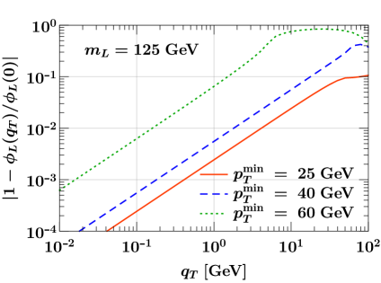
Figure -779: The two-particle phase space $\Phi_{L}(q_{T})$ relative to its Born-level value $\Phi_{L}(0)$ in the presence of a cut $p_{T}^{\rm min}$ on the individual momenta, as a function of the transverse momentum $q_{T}$.

The function $\Delta\Phi_{X}$ that captures the power corrections induced by the $p_{T}^{\rm min}$ cut is easily obtained by combining eqs. (3.1) and (3.24),

$$\Delta\Phi_{p_{T}^{\rm min}} =\Phi_{L}(q,p_{T}^{\rm min})-\Phi^{(0)}_{L}(q,p_{T}^{\rm min})={\mathcal{O}}\biggl{(}\frac{q_{T}}{Q}\frac{p_{T}^{\rm min}}{Q}\biggr{)}\,.$$ (3.27)

This linear dependence on $q_{T}$ translates into a relative power suppression of ${\mathcal{O}}(\lambda)$. Thus the power corrections in eq. (3.17) for a $p_{T}^{\rm min}$ cut have $m=1/2$ and scale as

$$\frac{\mathrm{d}\sigma^{(\mathrm{cuts})}(X)}{\mathrm{d}Q^{2}\mathrm{d}Y\mathrm{d}q_{T}^{2}}\sim\frac{1}{q_{T}^{2}}\frac{q_{T}}{Q}\,,\qquad\frac{\mathrm{d}\sigma^{(\mathrm{cuts})}(X)}{\mathrm{d}Q^{2}\mathrm{d}Y\mathrm{d}{\mathcal{T}}_{0}}\sim\frac{1}{{\mathcal{T}}_{0}}\sqrt{\frac{{\mathcal{T}}_{0}}{Q}}\,.$$ (3.28)

Hence, compared to the normal case of $m=1$, where the power corrections scale as $q_{T}^{2}/Q^{2}$ and ${\mathcal{T}}_{0}/Q$, corresponding to $\mathcal{O}(\lambda^{2})$, the power corrections induced by the kinematic selection cuts are enhanced as ${\mathcal{O}}(q_{T}/Q)$ and ${\mathcal{O}}(\sqrt{{\mathcal{T}}_{0}/Q})$. Intuitively, this arises from breaking the azimuthal symmetry that is present in the Born process, but which is explicitly broken by the recoil of the color-singlet system against the real emission. Hence, additional kinematic selection cuts will generically induce enhanced power corrections of $\mathcal{O}(\lambda)$.

3.3 Photon isolation

Next, we study the impact of photon isolation cuts on the power corrections. To disentangle this effect from the fiducial cuts considered in the previous section, we do not impose any other cuts besides the isolation. We define an isolation function $f_{\rm iso}(k,p_{\gamma})$ to evaluate to $1$ if the photon with momentum $p_{\gamma}$ is isolated from the emission with momentum $k$, and to evaluate to $0$ otherwise. The integrated phase space for diphoton production in the presence of such isolation, as defined in eq. (3.1), is given by

$$\Delta\Phi_{\rm iso}(Q,Y,k) =\int\Bigl{[}\mathrm{d}\Phi_{L}(p_{a}^{\prime}+p_{b}^{\prime}-k)\,f_{\rm iso}(k,p_{1}^{\prime})f_{\rm iso}(k,p_{2}^{\prime})-\mathrm{d}\Phi_{L}(p_{a}+p_{b})\Bigr{]}\,,$$ (3.29)

where as before $p_{1,2}^{\prime}$ are the momenta of the two photons, $p_{a,b}^{\prime}$ are the momenta of the incoming partons, and $k$ is the momentum of the real emission. To calculate the leading power behavior of eq. (3.29), it suffices to work in the singular limit of the phase space, where the photons are back to back with total momentum $q^{\mu}=(Q\cosh Y,0,0,Q\sinh Y)$. We parameterize their individual momenta by

$$p_{1}^{\mu} =p_{T}\bigl{(}\cosh(Y+\Delta y)\,,\,+\cos(\varphi)\,,\,+\sin(\varphi)\,,\,\sinh(Y+\Delta y)\bigr{)}\,,$$

$$p_{2}^{\mu} =p_{T}\bigl{(}\cosh(Y-\Delta y)\,,\,-\cos(\varphi)\,,\,-\sin(\varphi)\,,\,\sinh(Y-\Delta y)\bigr{)}\,,$$ (3.30)

where the rapidity difference $\Delta y$ and the photon transverse momenta $p_{T}$ are related by

$$\cosh(\Delta y)=\frac{Q}{2p_{T}}\,.$$ (3.31)

Using the expression eq. (3.21) for the diphoton phase space in the $q_{T}=0$ limit, we obtain

$$\Delta\Phi_{\rm iso}(Q,Y,k) =\frac{1}{32\pi^{2}}\int\frac{\mathrm{d}\Delta y}{\cosh^{2}\Delta y}\int_{-\pi}^{\pi}\!\mathrm{d}\varphi\,\bigl{[}f_{\rm iso}(k,p_{1})f_{\rm iso}(k,p_{2})-1\bigr{]}\,.$$ (3.32)

The calculation can be further simplified by assuming that both photons are well separated, such that their isolation cones never overlap with each other, and by assuming that the isolation energies for both photons are identically chosen as $E_{T}^{\rm iso}$. Since we work in the Born limit here, where $p_{T1}=p_{T2}\equiv p_{T}$, this assumption holds even if the isolation threshold is chosen proportional to the photon momentum, $E_{T}^{\rm iso}=\epsilon p_{T}$. This renders eq. (3.32) symmetric in both momenta $p_{1}$ and $p_{2}$, such that we obtain

$$\Delta\Phi_{\rm iso}(Q,Y,k) =\frac{1}{16\pi^{2}}\int\frac{\mathrm{d}\Delta y}{\cosh^{2}\Delta y}\int_{-\pi}^{\pi}\!\mathrm{d}\varphi\,\bigl{[}f_{\rm iso}(k,p_{1})-1\bigr{]}\,.$$ (3.33)

In the following, we evaluate eq. (3.33) for the different isolation techniques discussed in section 2.2 to deduce the resulting power corrections.

3.3.1 Fixed-cone isolation

We first study the fixed-cone isolation as defined in eq. (2.10), for which we have

$$f_{\rm cone}(k,p_{\gamma})=1-\theta(k_{T}-E_{T}^{\rm iso})\theta[R-d(k,p_{\gamma})]\,,$$ (3.34)

such that the photon is considered isolated unless the parton is inside the isolation cone of size $R$ and its transverse momentum exceeds the isolation energy $E_{T}^{\rm iso}$. Evaluating eq. (3.33) with eq. (3.34) gives

$$\Delta\Phi_{\rm cone}(Q,Y,k) =-\frac{\theta(k_{T}-E_{T}^{\rm iso})}{16\pi^{2}}\int\frac{\mathrm{d}\Delta y}{\cosh^{2}\Delta y}\int_{-\pi}^{\pi}\mathrm{d}\varphi\,\theta\Bigl{[}R-\sqrt{\varphi^{2}+(Y+\Delta y-y_{k})^{2}}\Bigr{]}$$

$$=-\frac{\theta(k_{T}-E_{T}^{\rm iso})}{8\pi^{2}}\int\frac{\mathrm{d}\Delta y}{\cosh^{2}\Delta y}\sqrt{R^{2}-(Y+\Delta y-y_{k})^{2}}\,.$$ (3.35)

Here, $y_{k}$ is the rapidity of $k$, and the range of the $\Delta y$ integral is kept implicit from the support of the square root. Note that eq. (3.3.1) is always negative, because it arises from an additional phase space restriction. For small $R^{2}\ll 1$, it can be approximated by

$$\Delta\Phi_{\rm cone}(Q,Y,k) =-\frac{R^{2}}{16\pi}\frac{\theta(k_{T}-E_{T}^{\rm iso})}{\cosh^{2}(Y-y_{k})}\times\bigl{[}1+{\mathcal{O}}(R^{2})\bigr{]}\,.$$ (3.36)

This correction vanishes as $R\to 0$, as in this limit the isolation turns off.

The nontrivial kinematic dependence of eq. (3.36) is entirely given by the denominator. To understand the induced power corrections, we first rewrite it as

$$\frac{1}{\cosh^{2}(Y-y_{k})}=\biggl{(}\frac{2e^{Y-y_{k}}}{1+e^{2(Y-y_{k})}}\biggr{)}^{2}=\frac{4k^{+}k^{-}}{(k^{-}e^{-Y}+k^{+}e^{Y})^{2}}\,.$$ (3.37)

Using the power counting from eqs. (3.9) and (3.10), we find in the $n$-collinear and soft limits the corrections

$$\text{$n$-collinear}:\quad k_{n}\sim Q\,(\lambda^{2},1,\lambda)\,, \quad\Rightarrow\quad\frac{1}{\cosh^{2}(Y-y_{k})}\quad\sim\quad{\mathcal{O}}(\lambda^{2})\,,$$

$$\text{soft}:\quad k_{s}\sim Q\,(\lambda,\lambda,\lambda)\,. \quad\Rightarrow\quad\frac{1}{\cosh^{2}(Y-y_{k})}\quad\sim\quad{\mathcal{O}}(\lambda^{0})\,,$$ (3.38)

and the corresponding ${\bar{n}}$-collinear and ultrasoft behavior follows trivially. Eq. (3.3.1) implies that only the (ultra)soft limit of eq. (3.36) can yield power corrections that are enhanced relative to the normal ${\mathcal{O}}(\lambda^{2})$ corrections intrinsic to the factorization, as the collinear corrections are always suppressed by (at least) ${\mathcal{O}}(\lambda^{2})$ as well.

From eqs. (3.36) and (3.3.1), it follows immediately that the power correction to the $q_{T}$ factorization from fixed-cone isolation is given by

$$\frac{\mathrm{d}\sigma^{\rm(cone)}(X)}{\mathrm{d}Q^{2}\mathrm{d}Y\mathrm{d}q_{T}^{2}}\sim\frac{R^{2}}{q_{T}^{2}}\theta(q_{T}-E_{T}^{\rm iso})\,.$$ (3.39)

Thus, while the scaling behavior is that of a leading-power term, $1/q_{T}^{2}\sim\lambda^{-2}$, this correction only contributes to $q_{T}\geq E_{T}^{\rm iso}$, and hence is suppressed for sufficiently large isolation energies. For a tight isolation, the effect can however become sizable.

The impact on the ${\mathcal{T}}_{0}$ subtraction is more involved, as it remains to integrate over $k$ against the ${\mathcal{T}}_{0}$ measurement. To do so, we first note that the effect of collinear emissions is always suppressed at least as ${\mathcal{T}}_{0}$ by virtue of eq. (3.3.1). Thus, an enhanced power correction can only result from the soft limit, which can be deduced by an explicit one-loop calculation. The bare expression for the soft limit without isolation effect is given by [74]

$$\frac{\mathrm{d}\sigma^{\rm soft}}{\mathrm{d}Q^{2}\mathrm{d}Y\mathrm{d}{\mathcal{T}}} =\frac{\mathrm{d}\sigma^{\mathrm{LO}}}{\mathrm{d}Q^{2}\mathrm{d}Y}\frac{\alpha_{s}\mathbf{C}}{\pi}\frac{e^{\epsilon\gamma_{E}}\mu^{2\epsilon}}{\Gamma(1-\epsilon)}\int_{0}^{\infty}\!\!\frac{\mathrm{d}k^{+}\mathrm{d}k^{-}}{(k^{+}k^{-})^{1+\epsilon}}$$ (3.40)

$$\quad\times\,\Bigl{[}\theta(e^{-Y}k^{-}-e^{Y}k^{+})\delta({\mathcal{T}}_{0}-e^{Y}k^{+})+\theta(e^{Y}k^{+}-e^{-Y}k^{-})\delta({\mathcal{T}}_{0}-e^{-Y}k^{-})\Bigr{]}\,,$$

where $\mathbf{C}=C_{F},C_{A}$ is the appropriate Casimir for quark annihilation and gluon fusion. Eq. (3.40) is the leading-power limit of the first line in eq. (3.1) without taking effects from $\Delta\Phi_{X}$ into account. By inserting eq. (3.36) into the integral in eq. (3.40), we can thus calculate the leading correction from the isolation. Letting $\epsilon\to 0$ and rescaling $k^{\pm}\to e^{\mp Y}k^{\pm}$ to remove any dependence on $Y$, we obtain

$$\frac{\mathrm{d}\sigma^{\rm(cone)}}{\mathrm{d}Q^{2}\mathrm{d}Y\mathrm{d}{\mathcal{T}}} =-\frac{\mathrm{d}\sigma^{\mathrm{LO}}}{\mathrm{d}Q^{2}\mathrm{d}Y}\times\frac{\alpha_{s}\mathbf{C}}{2\pi}\frac{R^{2}}{\pi}\int_{0}^{\infty}\frac{\mathrm{d}k^{-}}{({\mathcal{T}}_{0}+k^{-})^{2}}\theta[{\mathcal{T}}_{0}k^{-}-(E_{T}^{\rm iso})^{2}]\,\theta(k^{-}-{\mathcal{T}}_{0})$$

$$=-\frac{\mathrm{d}\sigma^{\mathrm{LO}}}{\mathrm{d}Q^{2}\mathrm{d}Y}\times\frac{\alpha_{s}\mathbf{C}}{2\pi}\frac{R^{2}}{\pi}\biggl{[}\frac{2}{{\mathcal{T}}_{0}}\theta({\mathcal{T}}_{0}-E_{T}^{\rm iso})+\frac{{\mathcal{T}}_{0}}{{\mathcal{T}}_{0}^{2}+(E_{T}^{\rm iso})^{2}}\theta(E_{T}^{\rm iso}-{\mathcal{T}}_{0})\biggr{]}\,.$$ (3.41)

In summary, the correction from fixed-cone isolation for ${\mathcal{T}}_{0}$ is given by

$$\frac{\mathrm{d}\sigma^{\rm(cone)}(X)}{\mathrm{d}Q^{2}\mathrm{d}Y\mathrm{d}{\mathcal{T}}_{0}}\sim\begin{cases}\displaystyle\frac{R^{2}}{{\mathcal{T}}_{0}}\biggl{(}\frac{{\mathcal{T}}_{0}}{E_{T}^{\rm iso}}\biggr{)}^{2}\qquad,\quad{\mathcal{T}}_{0}\leq E_{T}^{\rm iso}\,,\\ \displaystyle\frac{R^{2}}{{\mathcal{T}}_{0}}\hskip 64.01869pt,\quad{\mathcal{T}}_{0}>E_{T}^{\rm iso}\,.\end{cases}$$ (3.42)

For ${\mathcal{T}}_{0}>E_{T}^{\rm iso}$, this yields the leading-power $1/{\mathcal{T}}_{0}$ behavior, albeit suppressed by $R^{2}$, while for ${\mathcal{T}}_{0}<E_{T}^{\rm iso}$ this contribution is highly suppressed as $({\mathcal{T}}_{0}/E_{T}^{\rm iso})^{2}$.

3.3.2 Smooth-cone isolation

Next, we consider the smooth-cone isolation, eq. (2.12), using the definition of eq. (2.14) for $\chi(r)$. In this case, we have

$$f_{\rm smooth}(k,p_{\gamma}) =1-\theta\bigl{[}k_{T}-E_{T}^{\rm iso}(d(k,p_{\gamma})/R)^{2n}\bigr{]}\theta[R-d(k,p_{\gamma})]$$

$$=1-\theta\bigl{[}d_{\rm min}-d(k,p_{\gamma})\bigr{]}\,,$$ (3.43)

where

$$d_{\rm min}^{2}={\rm min}\bigl{\{}R^{2},R^{2}(k_{T}/E_{T}^{\rm iso})^{1/n}\bigr{\}}\,.$$ (3.44)

According to eq. (3.3.2), the photon is considered isolated unless the parton is inside the radiation cone and its transverse energy exceeds the threshold value, which itself depends on the distance between photon and parton. Eq. (3.33) in the presence of the isolation function eq. (3.3.2) can be evaluated similar to eq. (3.3.1) and yields

$$\Delta\Phi_{\rm smooth}(Q,Y,k) =-\frac{1}{16\pi^{2}}\int\frac{\mathrm{d}\Delta y}{\cosh^{2}(\Delta y)}\int_{-\pi}^{\pi}\mathrm{d}\varphi\,\theta\bigl{[}d_{\rm min}-d(k,\gamma)\bigr{]}$$

$$=-\frac{R^{2}}{16\pi}\frac{(k_{T}/E_{T}^{\rm iso})^{1/n}}{\cosh^{2}(Y-y_{k})}\times\bigl{[}1+{\mathcal{O}}(d_{\rm min}^{2})\bigr{]}\,,$$ (3.45)

where we expanded in small $d_{\rm min}$ and used that in the singular limit $k_{T}\ll Q$ the minimum in eq. (3.44) is always dominated by the second value.

From eqs. (3.3.2) and (3.3.1), it follows immediately that the power correction to the $q_{T}$ factorization from smooth-cone isolation is given by

$$\frac{\mathrm{d}\sigma^{\rm(smooth)}(X)}{\mathrm{d}Q^{2}\mathrm{d}Y\mathrm{d}q_{T}^{2}}\sim\frac{R^{2}}{q_{T}^{2}}\Bigl{(}\frac{q_{T}}{Q}\Bigr{)}^{1/n}\biggl{(}\frac{Q}{E_{T}^{\rm iso}}\biggr{)}^{1/n}\,.$$ (3.46)

Here, the overall $1/q_{T}^{2}$ arises from multiplying the leading-power singular with the isolation correction. This result should be compared to the inclusive power corrections, which scale as $q_{T}^{2}/Q^{2}$. Hence, while the absolute size of the isolation effect is suppressed by $R^{2}$, it is enhanced because the isolation energy $E_{T}^{\rm iso}$ is typically much smaller than the hard scale $Q$. For $n>1/2$ the scaling in $q_{T}$ is also parametrically enhanced compared to the inclusive case, and thus in practice the smooth-cone isolation can give sizable power corrections.

For ${\mathcal{T}}_{0}$, we have to distinguish that for collinear modes $k_{T}\sim\lambda Q\sim\sqrt{{\mathcal{T}}_{0}Q}$, while for ultrasoft modes $k_{T}\sim\lambda^{2}Q\sim{\mathcal{T}}_{0}$. Taking eq. (3.3.1) into account, we can deduce the dominant corrections depending on the isolation parameter $n$ from eq. (3.3.2) as

$$\frac{\mathrm{d}\sigma^{\rm(smooth)}(X)}{\mathrm{d}Q^{2}\mathrm{d}Y\mathrm{d}{\mathcal{T}}_{0}}\sim\begin{cases}\displaystyle\frac{R^{2}}{{\mathcal{T}}_{0}}\,\Bigl{(}\frac{{\mathcal{T}}_{0}}{Q}\Bigr{)}^{1+1/(2n)}\Bigl{(}\frac{Q}{E_{T}^{\rm iso}}\Bigr{)}^{1/n}\qquad,\quad n<1/2\,,\vspace{1ex}\\ \displaystyle\frac{R^{2}}{{\mathcal{T}}_{0}}\,\Bigl{(}\frac{{\mathcal{T}}_{0}}{Q}\Bigr{)}^{1/n}\Bigl{(}\frac{Q}{E_{T}^{\rm iso}}\Bigr{)}^{1/n}\hskip 44.10185pt,\quad n>1/2\,.\end{cases}$$ (3.47)

As for the $q_{T}$ case, there is an enhancement in $Q/E_{T}^{\rm iso}$ due to the typically small value for the isolation energy. Furthermore, compared to the inclusive case where the correction scales as ${\mathcal{O}}({\mathcal{T}}^{1})$, the scaling in ${\mathcal{T}}_{0}$ is parametrically enhanced for $n>1$. Hence, the relative parametric enhancement compared to the normal case turns out to be more severe for $q_{T}$ than ${\mathcal{T}}_{0}$.

The results in eqs. (3.46) and (3.47) hold for $q_{T}<E_{T}^{\rm iso}$ or ${\mathcal{T}}_{0}<E_{T}^{\rm iso}$, in which case the minimum in eq. (3.44) is given by the second term, which then induces the $k_{T}$ dependence of eq. (3.3.2). For the opposite case of $q_{T}>E_{T}^{\rm iso}$ or ${\mathcal{T}}_{0}>E_{T}^{\rm iso}$, the minimum in eq. (3.44) is instead given by $d_{\rm min}=R$, such that smooth-cone isolation reduces to fixed-cone isolation. Thus, we find that for $q_{T}>E_{T}^{\rm iso}$ or ${\mathcal{T}}_{0}>E_{T}^{\rm iso}$, smooth-cone isolation yields the same leading-power $1/q_{T}$ or $1/{\mathcal{T}}_{0}$ behavior as for fixed-cone isolation.

3.3.3 Harsh isolation.

Finally, we consider the harsh isolation defined in eq. (2.15), where

$$f_{\rm harsh}(k,p_{\gamma})=1-\theta\bigl{[}R-d(k,p_{\gamma})\bigr{]}\,,$$ (3.48)

which vetoes any radiation inside the isolation cone. The corresponding result for eq. (3.33) is easily obtained from eq. (3.36) by setting $E_{T}^{\rm iso}=0$,

$$\Delta\Phi_{\rm harsh}(Q,Y,k) =-\frac{R^{2}}{16\pi}\frac{\theta(k_{T})}{\cosh^{2}(Y-y_{k})}\times\bigl{[}1+{\mathcal{O}}(R^{2})\bigr{]}\,.$$ (3.49)

The induced correction then follows directly from eqs. (3.39) and (3.42) as

$$\frac{\mathrm{d}\sigma^{\rm(harsh)}(X)}{\mathrm{d}Q^{2}\mathrm{d}Y\mathrm{d}q_{T}^{2}}\sim\frac{R^{2}}{q_{T}^{2}}\,,\qquad\frac{\mathrm{d}\sigma^{\rm(harsh)}(X)}{\mathrm{d}Q^{2}\mathrm{d}Y\mathrm{d}{\mathcal{T}}_{0}}\sim\frac{R^{2}}{{\mathcal{T}}_{0}}\,.$$ (3.50)

This is a leading power (singular) effect, as the harsh isolation completely removes part of the real emission phase space, namely the vicinity of the two photons, and thus immediately breaks both factorization theorems, which rely on an analytic integration over the full emission phase space.

3.4 Factorization violation in photon isolation

In this section, we briefly discuss a potential source for factorization violation for isolation methods when not carefully applying the isolation procedure. In general, one only keeps events that satisfy the chosen isolation criterion. The remaining events can then still contain jets, as defined by a suitable jet algorithm applied after the isolation, that are inside or overlapping the isolation cones, e.g. if the jets are sufficiently soft.

Since any jet inside the isolation cone will typically be quite soft, as part of the overall isolation procedure one can in principle also remove any jets inside the isolation cone from further consideration, i.e., the events are kept but the jets are not further considered for the calculation of physical quantities, e.g. jet selection cuts. This approach is for example proposed in the original definition of smooth-cone isolation in ref. [90].

For the purpose of the subtractions, it is however crucial to keep all reconstructed jets, or more generally all emissions, for the determination of the resolution variable ${\mathcal{T}}$. More generally, this applies to employing any factorization theorem, irrespective of whether it is used for subtractions or resummation of large logarithms. For example, recall the definition for $0$-jettiness, see eq. (2.2)

$${\mathcal{T}}_{0}=\sum_{i}{\rm min}\bigl{\{}k_{i}^{+}e^{Y}\,,\,k_{i}^{-}e^{-Y}\bigr{\}}\,.$$ (3.51)

Here, the sum $i$ runs over all particles $i$ in the final state, only excluding the color-singlet final state, which is critical for the derivation of the ${\mathcal{T}}_{0}$ factorization theorem. Excluding any emissions inside the isolation cones from the sum in eq. (3.51) would thus change the definition of ${\mathcal{T}}_{0}$ and immediately violate the ${\mathcal{T}}_{0}$ factorization theorem. For example, at one loop, where one has only one real emission, excluding jets inside the isolation cones is equivalent to excluding the emission. As far as calculating ${\mathcal{T}}_{0}$ is concerned, this exactly corresponds to the harsh isolation defined in eq. (2.15). As discussed in section 3.3.3, this induces leading-power corrections, which exactly corresponds to breaking the factorization.

For $q_{T}$ subtraction, one can trivially avoid this problem by determining $q_{T}$ directly from the color-singlet final state $L$, i.e. $q_{T}\equiv q_{T,L}$. On the other hand, if $q_{T}$ is obtained from the sum of all real emissions, $q_{T}=|\sum_{i}\vec{k}_{T,i}|$, then as for ${\mathcal{T}}_{0}$, the sum over $i$ must not exclude emissions inside the isolation cones to not violate the factorization.

Lastly, we point out that this leads to a trivial yet dangerous pitfall in the calculation of power corrections. For example, to calculate the NLO cross section for $pp\to H$ using ${\mathcal{T}}_{0}$ subtractions, one would use $pp\to H+j$ at LO to calculate the power corrections or the above-cut contributions in the slicing approach. Naively applying the smooth-cone isolation including the discussed treatment of jets to the resulting $H+j$ events, one would classify all events where the emitted parton falls inside the isolation cone as $0$-jet events, which depending on the used tool might be discarded in a $pp\to H+j$ calculation, where at least one jet is required at Born level. We have explicitly checked that this is the case for MCFM8 [98, 99, 100, 101]. To not violate the subtraction method, it is however mandatory to keep all such events, and we have turned off this mechanism in MCFM8 to obtain the correct results for our numerical studies in section 4. (This does not impact the NLO calculations in MCFM8 itself, which keeps the $H+j$ events that are otherwise classified as $0$-jet events.)

4 Numerical results

To validate our findings and assess the importance of the discussed power corrections, we numerically study the $q_{T}$ and ${\mathcal{T}}_{0}$ spectrum at NLO₀, for direct diphoton production, $pp\to{\gamma\gamma}$, and for gluon-fusion Higgs production in the diphoton decay mode, $pp\to H\to{\gamma\gamma}$, using different photon acceptance cuts and isolation methods. In all cases, we compare the full QCD result obtained from MCFM8 [98, 99, 100, 101] against the predicted singular spectrum obtained from SCETlib [102]. For both processes, we use the PDF4LHC15_nnlo_mc [103] PDF set and fix the factorization and renormalization scales to $\mu_{f}=\mu_{r}=m_{H}=125~{}\,\mathrm{GeV}$.

To present our results, we normalize the cross section with the cuts $X$ to the LO cross section $\sigma^{\mathrm{LO}}(X^{\mathrm{LO}})$ and split it into singular and nonsingular contributions,

$$\frac{\mathrm{d}\hat{\sigma}^{\rm full}(X)}{\mathrm{d}{\mathcal{T}}}\equiv\frac{1}{\sigma^{\mathrm{LO}}(X^{\mathrm{LO}})}\frac{\mathrm{d}\sigma(X)}{\mathrm{d}{\mathcal{T}}} =\frac{\mathrm{d}\hat{\sigma}^{\rm sing}}{\mathrm{d}{\mathcal{T}}}+\frac{\mathrm{d}\hat{\sigma}^{\rm nons}(X)}{\mathrm{d}{\mathcal{T}}}$$

$$=\frac{\mathrm{d}\hat{\sigma}^{\rm sing}}{\mathrm{d}{\mathcal{T}}}+\frac{\mathrm{d}\hat{\sigma}^{\rm nons}}{\mathrm{d}{\mathcal{T}}}+\frac{\mathrm{d}\Delta\hat{\sigma}^{\rm nons}(X)}{\mathrm{d}{\mathcal{T}}}\,.$$ (4.1)

Here, $X^{\mathrm{LO}}$ indicates that the cuts only act on the Born kinematics of the produced diphoton system, which in particular implies that there are no isolation effects. For the normalized singular cross section $\hat{\sigma}^{\rm sing}=\sigma^{(0)}(X^{\mathrm{LO}})/\sigma^{\mathrm{LO}}(X^{\mathrm{LO}})$, the dependence on $X^{\mathrm{LO}}$ fully cancels since the LP cross section only depends on the Born-level cuts $X^{\mathrm{LO}}$. The nonsingular cross section $\hat{\sigma}^{\rm nons}(X)=\hat{\sigma}^{\rm full}(X)-\hat{\sigma}^{\rm sing}$ contains all power-suppressed contributions. In the second line, we have further split this piece into the power corrections $\mathrm{d}\hat{\sigma}^{\rm nons}$ that are already present without additional cuts and the additional power corrections $\mathrm{d}\Delta\hat{\sigma}^{\rm nons}(X)$ that are induced by the cuts $X$. Comparing these two thus gives a direct indication of their relative importance.

For Higgs production, we work in the on-shell limit where the invariant mass is fixed to $Q=m_{H}=125~{}\,\mathrm{GeV}$, while for diphoton production we restrict $Q=m_{\gamma\gamma}=120{-}130~{}\,\mathrm{GeV}$ such that $m_{\gamma\gamma}\sim m_{H}$. In both cases, we are inclusive over the rapidity $Y$ of the final state. For direct photon production, we furthermore restrict ourselves to the $q\bar{q}\to{\gamma\gamma}+g$ channel to avoid contributions from the fragmentation process $qg\to\gamma+q(\to q+\gamma)$. This allows us to obtain results without any photon isolation or fragmentation functions, and thus compare the results with and without photon isolation. Since direct diphoton production is divergent in the forward limit $p_{T}\to 0$, we always impose selection cuts $p_{T}>p_{T}^{\rm min}=25~{}\,\mathrm{GeV}$ to obtain a finite cross section. This is not necessary for Higgs production, which we can also consider without any photon selection cuts.

4.1 Kinematic selection cuts

We first study the effect of fiducial cuts by comparing $pp\to H\to{\gamma\gamma}$ with a lower cut on the photon transverse momenta, $p_{T}>p_{T}^{\rm min}=25~{}\,\mathrm{GeV}$, to the inclusive case without such a cut. As mentioned above, the same comparison cannot be performed for direct diphoton production, since it diverges in the forward limit.

In figure -778, we show the $q_{T}$ spectrum (left) and ${\mathcal{T}}_{0}$ spectrum (right). The red solid curve shows the full spectrum $\hat{\sigma}^{\rm full}$ for reference. The blue dashed curve shows the nonsingular spectrum $\hat{\sigma}^{\rm nons}$ without the $p_{T}^{\rm min}$ cut. Its slope shows the ${\mathcal{O}}(q_{T}^{2})$ and ${\mathcal{O}}({\mathcal{T}}_{0})$ suppression of the nonsingular corrections without any cuts. For ${\mathcal{T}}_{0}$, the nonsingular terms change sign around ${\mathcal{T}}_{0}\approx 30\,\mathrm{GeV}$, which due to the logarithmic scale leads to the kink of the blue-dashed curve. The green dotted curve shows the additional nonsingular corrections $\Delta\hat{\sigma}^{\rm nons}$ from applying the $p_{T}^{\rm min}$ cut on the photons. Its less steep slope shows the ${\mathcal{O}}(q_{T})$ and ${\mathcal{O}}(\sqrt{{\mathcal{T}}_{0}})$ scaling, consistent with the result of section 3.2. The cut-induced corrections dominate up to rather large values $q_{T}\lesssim 5~{}\,\mathrm{GeV}$ and ${\mathcal{T}}_{0}\lesssim 1~{}\,\mathrm{GeV}$, and hence have a significant impact for both subtractions and resummation applications. At typical subtraction cutoffs $q_{T}\lesssim 1~{}\,\mathrm{GeV}$ the cut-induced corrections are almost an order of magnitude enhanced, while for ${\mathcal{T}}_{0}\lesssim 0.1\,\mathrm{GeV}$ they are enhanced by a factor of two.

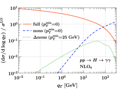
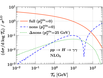
Figure -778: Comparison of Higgs production with and without a cut on the photon transverse momenta for the $q_{T}$ spectrum (left) and the ${\mathcal{T}}_{0}$ spectrum (right).

4.2 Photon isolation cuts

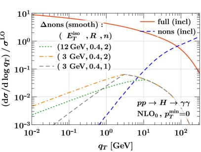
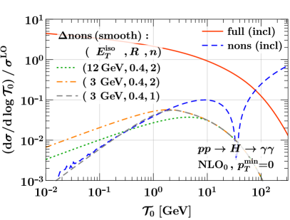
Figure -777: Power corrections in $H\to{\gamma\gamma}$ with smooth-cone isolation for the $q_{T}$ spectrum (left) and the ${\mathcal{T}}_{0}$ spectrum (right). The red and blue dashed lines show the full and nonsingular results without isolation. The other curves show the additional nonsingular corrections induced by the isolation for different isolation parameters.

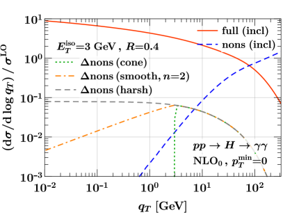
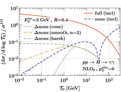
(a) $pp\to H\to{\gamma\gamma}$ with $p_{T}^{\rm min}=0$.

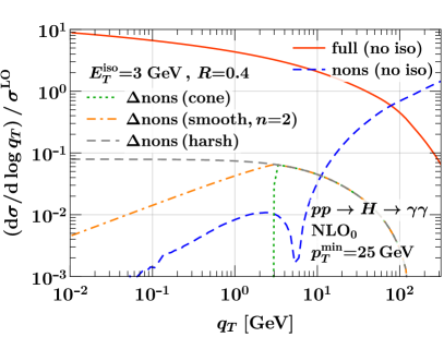
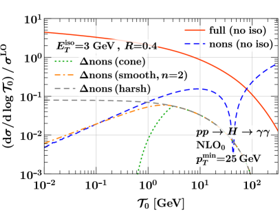
(b) $pp\to H\to{\gamma\gamma}$ with $p_{T}^{\rm min}=25~{}\,\mathrm{GeV}$.

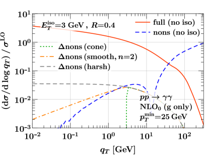
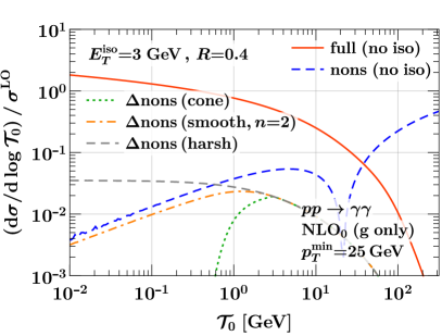
(c) $q\bar{q}\to{\gamma\gamma}$ with $p_{T}^{\rm min}=25~{}\,\mathrm{GeV}$ and $m_{{\gamma\gamma}}\in[120,130]~{}\,\mathrm{GeV}$.

Figure -776: Comparison of the power corrections for the $q_{T}$ spectrum (left) and the ${\mathcal{T}}_{0}$ spectrum (right) for different photon isolation methods. The red and blue curves show the full result and nonsingular corrections without any isolation. The other curves show the additional nonsingular corrections induced by the isolation using fixed-cone isolation (green), smooth-cone isolation (orange), and harsh isolation (gray).

Next, we consider the effect of photon isolation cuts. We begin by illustrating the dependence of the power corrections for smooth-cone isolation on the isolation parameters, as given in eqs. (3.46) and (3.47). To not mix effects from the photon isolation and kinematic acceptance cuts, we restrict ourselves to Higgs production with $p_{T}^{\rm min}=0$. Since the induced power corrections depend trivially on the isolation radius $R$, $\Delta\hat{\sigma}\sim R^{2}$, we fix $R=0.4$ and only vary the isolation energy $E_{T}^{\rm iso}$ and the parameter $n$. We consider the three choices

green dotted: $$E_{T}^{\rm iso}=12~{}\,\mathrm{GeV},~{}R=0.4,~{}n=2\,,$$

orange dot-dashed: $$E_{T}^{\rm iso}=3~{}\,\mathrm{GeV},~{}\,~{}R=0.4,~{}n=2\,,$$

gray dashed: $$E_{T}^{\rm iso}=3~{}\,\mathrm{GeV},~{}\,~{}R=0.4,~{}n=1\,,$$ (4.2)

for which we show in figure -777 the $q_{T}$ and ${\mathcal{T}}_{0}$ spectra. The red solid curve shows the full result $\hat{\sigma}^{\rm full}$ for reference. The blue dashed curve shows the nonsingular corrections $\hat{\sigma}^{\rm nons}$ without isolation cuts. Its slope shows the normal ${\mathcal{O}}(q_{T}^{2})$ and ${\mathcal{O}}({\mathcal{T}}_{0})$ suppression (and similar to figure -778 the kink around ${\mathcal{T}}_{0}\approx 30\,\mathrm{GeV}$ is due to a sign change). The additional curves as stated in eq. (4.2) show the additional nonsingular correction $\Delta\hat{\sigma}^{\rm nons}$ from the different isolations requirements, which for small $q_{T}$ and ${\mathcal{T}}_{0}$ obey the ${\mathcal{O}}(q_{T}^{1/n})$ and ${\mathcal{O}}({\mathcal{T}}_{0}^{1/n})$ behavior as predicted by eqs. (3.46) and (3.47). The gap between the green-dotted and orange-dot-dashed curves corresponds to a factor of $2$, correctly reflecting the scaling of the power corrections with $\sqrt{E_{T}^{\rm iso}}$ for $n=2$. Above $q_{T}\geq E_{T}^{\rm iso}$ and ${\mathcal{T}}_{0}\geq E_{T}^{\rm iso}$, the different isolations agree as in this limit each emission that falls into an isolation cone is necessarily too energetic to be allowed, independently of the chosen isolation method. In this region, the isolation is in fact a leading-power effect, while below this region it becomes a power correction which leads to the kink at $q_{T}=E_{T}^{\rm iso}$ and ${\mathcal{T}}_{0}=E_{T}^{\rm iso}$. (For ${\mathcal{T}}_{0}$, this follows from the explicit calculation presented in section 3.3.1.)

Overall, we find that in each case the smooth-cone isolation yields large additional corrections, which as expected from the relative scaling are significantly enhanced compared to the normal power corrections (blue dashed), and which exhibit a very slow convergence to zero for $q_{T}\to 0$ or ${\mathcal{T}}_{0}\to 0$. The relative enhancement is particularly severe for $q_{T}$, easily exceeding an order of magnitude for $q_{T}\lesssim 1\,\mathrm{GeV}$. This suggests that calculations of processes involving smooth-cone isolation with $q_{T}$ or ${\mathcal{T}}_{N}$ subtractions should prefer a loose isolation, which however goes opposite to the recommendation of refs. [95, 96, 93] to employ tight cuts in order for smooth-cone isolation to yield similar results as fixed-cone isolation.

In figure -776, we compare fixed-cone, smooth-cone, and harsh isolations. The top (middle) row shows Higgs production in the diphoton decay mode with a cut $p_{T}^{\rm min}=0$ ($p_{T}^{\rm min}=25~{}\,\mathrm{GeV}$) on the photons. The bottom row shows direct diphoton production $pp\to{\gamma\gamma}$ with $p_{T}^{\rm min}=25~{}\,\mathrm{GeV}$, where only the $q\bar{q}\to\gamma\gamma g$ channel is taken into account to avoid fragmentation contributions. In all figures, the red solid curves show the full result $\hat{\sigma}^{\rm full}$ for reference. The blue dashed curves show the nonsingular corrections $\hat{\sigma}^{\rm nons}$ without any isolation but including the $p_{T}^{\rm min}$ cut. The additional nonsingular corrections induced by the isolation are shown in green dotted for fixed-cone isolation, orange dot-dashed for smooth-cone isolation with $n=2$, and in gray dashed for harsh isolation. In each case, we use $R=0.4$ and $E_{T}^{\rm iso}=3~{}\,\mathrm{GeV}$.

For the $q_{T}$ spectrum, we see that cone isolation has no power corrections for $q_{T}\leq E_{T}^{\rm iso}$, and likewise almost negligible corrections to the ${\mathcal{T}}_{0}$ spectrum for ${\mathcal{T}}_{0}\leq E_{T}^{\rm iso}$, consistent with our findings in section 3.3. In contrast, smooth-cone isolation shows the predicted much weaker suppression of ${\mathcal{O}}(q_{T}^{1/n})$ and ${\mathcal{O}}({\mathcal{T}}_{0}^{1/n})$. As a result, it yields in all cases sizable additional power corrections, which for $q_{T}$ clearly dominate over the corrections without isolation, both with and without the $p_{T}^{\rm min}$ cut. For ${\mathcal{T}}_{0}$, they are of the same order as the corrections induced by the $p_{T}^{\rm min}$ cut, while for $p_{T}^{\rm min}=0$ the isolation again dominates over the inclusive nonsingular corrections. Finally, the harsh isolation yields an almost constant correction on the logarithmic plot, which translates into leading-power correction in $1/q_{T}$ and $1/{\mathcal{T}}_{0}$. Note that these are not integrable as $q_{T},{\mathcal{T}}_{0}\to 0$, reflecting the factorization violation from the infrared-unsafe isolation procedure.

5 ${\mathcal{T}}_{N}$ subtractions including measurement cuts

In this section, we discuss how all cut-induced power corrections can be accounted for exactly in the subtraction procedure. Our starting point are differential ${\mathcal{T}}_{N}$ subtractions [39], using which the cross section with a measurement $X$ is given by

$$\sigma(X) =\sigma^{\mathrm{sub}}(X,\tau_{\mathrm{off}})+\int\!\mathrm{d}\tau\,\biggl{[}\frac{\mathrm{d}\sigma(X)}{\mathrm{d}\tau}-\frac{\mathrm{d}\sigma^{\mathrm{sub}}(X)}{\mathrm{d}\tau}\theta(\tau<\tau_{\mathrm{off}})\biggr{]}$$

$$=\sigma^{\mathrm{sub}}(X,\tau_{\mathrm{off}})+\int^{\tau_{\mathrm{off}}}\!\mathrm{d}\tau\,\biggl{[}\frac{\mathrm{d}\sigma(X)}{\mathrm{d}\tau}-\frac{\mathrm{d}\sigma^{\mathrm{sub}}(X)}{\mathrm{d}\tau}\biggr{]}+\int_{\tau_{\mathrm{off}}}\!\mathrm{d}\tau\,\frac{\mathrm{d}\sigma(X)}{\mathrm{d}\tau}\,.$$ (5.1)

As in section 2.1, $\tau$ stands for any (dimensionless) $N$-jet resolution variable for which a LP factorization theorem is known. The differential subtraction term $\mathrm{d}\sigma^{\mathrm{sub}}(X)/\mathrm{d}\tau$ captures the leading-power singularities for $\tau\to 0$, which means it satisfies

$$\frac{\mathrm{d}\sigma^{\mathrm{sub}}(X)}{\mathrm{d}\tau}=\frac{\mathrm{d}\sigma^{(0)}(X)}{\mathrm{d}\tau}\bigl{[}1+\mathcal{O}(\tau)\bigr{]}\,,$$ (5.2)

such that the integrand in square brackets in eq. (5) is a power correction with at most integrable singularities for $\tau\to 0$, and so the integral can be carried out numerically. Since the integral exists and is finite, the point $\tau=0$ is irrelevant, which means the integrand is never evaluated at $\tau=0$. Hence, the full result for $\mathrm{d}\sigma(X)/\mathrm{d}\tau$ is only needed for nonzero $\tau>0$ and thus reduces to performing the NLO Born+1-parton calculation. Similarly the distributional structure of $\mathrm{d}\sigma^{\mathrm{sub}}(X)/\mathrm{d}\tau$ at $\tau=0$ is not needed for the differential subtraction terms, which are fully known to N³LO for both $q_{T}$ and ${\mathcal{T}}_{0}$ subtractions [51]. The first term in eq. (5) is the cumulant of $\mathrm{d}\sigma^{\mathrm{sub}}(X)/\mathrm{d}\tau$ up to $\tau_{\mathrm{off}}$. Its evaluation does require the full distributional structure of $\mathrm{d}\sigma^{\mathrm{sub}}(X)/\mathrm{d}\tau$.

Note that in principle the integrand does need to be sampled arbitrarily close to $\tau=0$, but due to the subtraction the contribution from a region $\tau<\delta$ is of $\mathcal{O}(\delta)$. This is similar to the fact that even in a fully local subtraction method the real-emission phase-space formally needs to be sampled arbitrarily close to the IR-singular region, but the subtractions ensure that the total subtracted integrand is well-behaved, so the contribution from a region of size $\delta$ around the singularity only contributes an amount of $\mathcal{O}(\delta)$. Letting $\delta\to 0$ still requires evaluating the real-emissions matrix elements arbitrarily close to the singularity, and to avoid numerical instabilities due to arbitrarily large numerical cancellations one always has a technical cutoff $\delta$ that cuts out the actual singular points of phase space.

The parameter $\tau_{\mathrm{off}}$ determines the range over which the subtractions act, and by taking $\tau_{\mathrm{off}}\sim 1$ there are no large numerical cancellations between the first and second term in eq. (5). (In the context of resummation, $\tau_{\mathrm{off}}$ corresponds to where the $\tau$ resummation is turned off.) The slicing method described in section 2.1 is obtained from eq. (5) by taking $\tau_{\mathrm{off}}=\tau_{\mathrm{cut}}$, see eq. (2.1). In this case, the integral below $\tau_{\mathrm{off}}=\tau_{\mathrm{cut}}$ corresponds to $\Delta\sigma(X,\tau_{\mathrm{cut}})$ and is neglected, which induces the power corrections. In contrast, eq. (5) is exact and involves no neglected power corrections.

The practical challenge in implementing eq. (5) is that the NLO calculation for $\mathrm{d}\sigma(X)/\mathrm{d}\tau$ has to be obtained as a function of $\tau$. In general this is not easy as it requires to organize the integration over the real-emission phase space in such a way that $\tau$ is preserved, which by default is not the case for standard NLO subtractions. For a more detailed discussion we refer to ref. [39].

To make the differential subtractions more viable in practice, we can follow the same basic strategy as in section 3 to separate the different sources of power corrections. We first note that the LP singular contribution only depends on the Born phase space. That is, the factorization theorem for $\tau$ is always fully differential in the Born phase space, which involves choosing a specific set of kinematic variables to parametrize the Born phase space. The measurement $X$ is then evaluated on this reference Born phase space. In other words, constructing $\mathrm{d}\sigma^{(0)}(X)/\mathrm{d}\tau$ involves choosing a Born projection $\hat{\Phi}_{N}(\Phi_{N+k})$ from the real-emission phase-space with $k$ additional emissions, $\Phi_{N+k}$, to the Born phase space, $\Phi_{N}$. For color-singlet production ($N=0$), a typical choice is to use $Q$ and $Y$ as the Born variables, as we did in section 3 above. The LP measurement function that actually enters in $\mathrm{d}\sigma^{(0)}(X)/\mathrm{d}\tau$ is then given by

$$f_{X}^{(0)}(\Phi_{N+k})=f_{X}[\hat{\Phi}_{N}(\Phi_{N+k})]\,.$$ (5.3)

For color-singlet production at NLO, this is precisely the LP term on the right-hand side of eq. (3.13). Denoting this LP measurement by $X^{(0)}$, we therefore have

$$\frac{\mathrm{d}\sigma^{\mathrm{sub}}(X)}{\mathrm{d}\tau}\equiv\frac{\mathrm{d}\sigma^{\mathrm{sub}}(X^{(0)})}{\mathrm{d}\tau}\,,\qquad\sigma^{\mathrm{sub}}(X,\tau_{\mathrm{off}})\equiv\sigma^{\mathrm{sub}}(X^{(0)},\tau_{\mathrm{off}})\,.$$ (5.4)

Next, we can consider the full cross section but with the measurement replaced by this LP Born reference measurement, $\mathrm{d}\sigma(X^{(0)})/\mathrm{d}\tau$. By adding and subtracting it, we can rewrite eq. (5) as

$$\sigma(X) =\sigma^{\mathrm{sub}}(X^{(0)},\tau_{\mathrm{off}})+\int\!\mathrm{d}\tau\,\biggl{[}\frac{\mathrm{d}\sigma(X^{(0)})}{\mathrm{d}\tau}-\frac{\mathrm{d}\sigma^{\mathrm{sub}}(X^{(0)})}{\mathrm{d}\tau}\theta(\tau<\tau_{\mathrm{off}})\biggr{]}+\int\!\mathrm{d}\tau\,\frac{\mathrm{d}\sigma(X-X^{(0)})}{\mathrm{d}\tau}$$

$$\equiv\sigma(X^{(0)})+\sigma(X-X^{(0)})\,.$$ (5.5)

We have now isolated the two different sources of power corrections. The sum of the first two terms in the first line of eq. (5) is the calculation of the reference cross section $\sigma(X^{(0)})$ using differential $\tau$ subtractions. Since it involves the same reference measurement $X^{(0)}$ everywhere, the difference $\mathrm{d}\sigma(X^{(0)})-\mathrm{d}\sigma^{\mathrm{sub}}(X^{(0)})$ does not involve any cut-induced power corrections, hence reducing the problem of power corrections to the normal and well-studied case, and for which the power corrections can be systematically calculated if necessary [70, 71, 72, 73, 74, 75, 76]. In particular, if the implementation of the differential $\tau$ subtractions proves too difficult in practice, this contribution could be calculated with the slicing approach (see below).

The last term in eq. (5) amounts to measuring the difference between $X$ and $X^{(0)}$ on the full cross section. Here we exploited that the difference of the two cross sections can be combined into a single cross section, as the only difference lies in the measurement,

$$\int\!\mathrm{d}\tau\biggl{[}\frac{\mathrm{d}\sigma(X)}{\mathrm{d}\tau}-\frac{\mathrm{d}\sigma(X^{(0)})}{\mathrm{d}\tau}\biggr{]}=\int\!\mathrm{d}\tau\,\frac{\mathrm{d}\sigma(X-X^{(0)})}{\mathrm{d}\tau}=\sigma(X-X^{(0)})\,.$$ (5.6)

That is, $\sigma(X-X^{(0)})$ contains the difference of the full and LP measurement functions, $f_{X}(\Phi_{N+k})-f_{X}^{(0)}(\Phi_{N+k})$. For example, for color-singlet production at NLO, $\mathrm{d}\sigma(X-X^{(0)})$ is precisely given by eq. (3.1). Since for any infrared safe $X$ this measurement difference vanishes in the singular limit, $\sigma(X-X^{(0)})$ still amounts to effectively performing a Born+1-parton calculation at one lower order. It contains all cut-induced power corrections, which as we discussed can be potentially large, and it should therefore be treated exactly. Since it can be formulated as a specific choice of measurement, it can be implemented straightforwardly into existing NLO calculations. Once this is done, the explicit dependence on $\tau$ disappears. (In general it might still be implicit through the choice of $X^{(0)}$.) One might say that the reference cross section $\mathrm{d}\sigma(X^{(0)})$ in eq. (5.6) effectively acts as a fully local subtraction term. However, this is somewhat misleading, since the IR singularities do not cancel in the difference of two singular contributions. Rather, they are simply regulated by performing an IR-safe Born+1-parton measurement.

When performing the calculation of $\sigma(X-X^{(0)})$ one might still have to integrate near the singular region of phase space, but only to the extent to which the full measurement is sensitive to, which is the best one can hope for. For example, if $X$ contains isolation cuts, then $X^{(0)}$ will contain no isolation cuts. The difference $X-X^{(0)}$ then measures the cross section that is removed by the isolation, which is sensitive to real emissions with energies down to $E_{T}^{\rm iso}$, while below that the difference of the two measurements explicitly vanishes. For selection cuts, one can still get sensitive to arbitrarily soft emissions, e.g., when measuring the $p_{T}$ of the photons in $H\to\gamma\gamma$ very close to the Born limit $p_{T}=m_{H}/2$. However, this is a well-known feature of such cuts and inherent to the measurement itself and not related the subtraction method.

From the above discussion, we can also see the connection to the projection-to-Born method [31]. It amounts to the special case where the reference cross section $\mathrm{d}\sigma(X^{(0)})$ is known analytically or from some other calculation, while the last term is precisely the effective Born+1-parton calculation that also appears in the projection-to-Born method. In other words, the projection-to-Born method is simply the statement that $\sigma(X)$ can be calculated as

$$\sigma(X)=\sigma(X^{(0)})+\sigma(X-X^{(0)})\,,$$ (5.7)

when the full cross section $\sigma(X^{(0)})$ for some reference measurement $X^{(0)}$ is already known, and the correction term $\sigma(X-X^{(0)})$ is calculated by evaluating the $X-X^{(0)}$ measurement for the lower-order Born+1-parton calculation as described above.

To conclude, we note that if the reference cross section $\sigma(X^{(0)})$ is obtained via a global $\tau$ slicing, one can of course combine both Born+1-parton calculations into a single one,

$$\sigma(X) =\sigma^{\mathrm{sub}}(X^{(0)},\tau_{\mathrm{cut}})+\sigma[X-X^{(0)}\theta(\tau<\tau_{\mathrm{cut}})]+\Delta\sigma(X^{(0)},\tau_{\mathrm{cut}})\,.$$ (5.8)

This makes it explicit that in contrast to eq. (2.1), here the power corrections $\Delta\sigma(X^{(0)},\tau_{\mathrm{cut}})$ are only those for the chosen reference measurement. The cut-induced power corrections are accounted for by the Born+1-parton calculation in the second term, because it correctly captures the difference $X-X^{(0)}$ below $\tau_{\mathrm{cut}}$.

6 Conclusions

We have studied the impact of kinematic selection cuts and isolation requirements for leptons and photons on the $q_{T}$ and $N$-jettiness subtraction methods. Using a simplified one-loop calculation, we analytically determined the scaling of power corrections induced by these cuts including their dependence on the isolation method and its parameters. We find that both selection cuts and isolation induce additional power corrections that are parametrically enhanced relative to the usual, cut-independent power corrections inherent to the $q_{T}$ and ${\mathcal{T}}_{0}$ factorization theorems. We have also discussed how the cut effects can be fully incorporated into the subtraction, thereby avoiding the additional power corrections, by employing differential subtractions for them instead of a global slicing method.

To summarize our key findings, we expand the differential $q_{T}$ and ${\mathcal{T}}_{0}$ spectra as

$$\frac{\mathrm{d}\sigma(X)}{\mathrm{d}Q^{2}\mathrm{d}Y\mathrm{d}q_{T}^{2}} =\frac{\mathrm{d}\sigma^{(0)}(X)}{\mathrm{d}Q^{2}\mathrm{d}Y\mathrm{d}q_{T}^{2}}\times\Bigl{[}1+{\mathcal{O}}\bigl{[}(q_{T}^{2}/Q^{2})^{m}\bigr{]}\Bigr{]}\,,$$

$$\frac{\mathrm{d}\sigma(X)}{\mathrm{d}Q^{2}\mathrm{d}Y\mathrm{d}{\mathcal{T}}_{0}} =\frac{\mathrm{d}\sigma^{(0)}(X)}{\mathrm{d}Q^{2}\mathrm{d}Y\mathrm{d}{\mathcal{T}}_{0}}\times\Bigl{[}1+{\mathcal{O}}\bigl{[}({\mathcal{T}}_{0}/Q)^{m}\bigr{]}\Bigr{]}\,,$$ (6.1)

where $\sigma^{(0)}$ are the leading-power limits predicted by the factorization theorems. We find the following power corrections in the square brackets in eq. (6) for typical selection and isolation cuts:

• For inclusive processes without any cuts, one has $m=1$.

• A typical $p_{T}>p_{T}^{\rm min}$ selection cut for photons or leptons yields enhanced power corrections with $m=1/2$ and proportional to $\sim p_{T}^{\rm min}/Q$. Since this arises from breaking azimuthal symmetry that is only present in the Born process, we expect a similar enhancement for generic fiducial cuts.

• All photon isolation methods yield leading-power corrections ($m=0$) for $q_{T}>E_{T}^{\rm iso}$ and ${\mathcal{T}}_{0}>E_{T}^{\rm iso}$, respectively, which are proportional to the size of the isolation cone $\sim{\mathcal{O}}(R^{2})$.

• At one loop, fixed-cone isolation induces no corrections for $q_{T}<E_{T}^{\rm iso}$ and highly suppressed corrections ($m=2$) for ${\mathcal{T}}_{0}<E_{T}^{\rm iso}$. At higher orders one can expect nontrivial corrections also below $E_{T}^{\rm iso}$, which should be power suppressed.

• Smooth-cone isolation as defined in eq. (2.14) yields power corrections scaling as $m=1/(2n)$ for $q_{T}$ and $m=1/n$ for ${\mathcal{T}}_{0}$, respectively. They are further enhanced by an overall factor $(Q/E_{T}^{\rm iso})^{1/n}$.

In general, tight cuts can thus yield significantly enhanced power corrections. The enhancement is most severe for smooth-cone isolation with $q_{T}$ subtractions. We have numerically verified and studied these findings for the examples of $pp\to H\to{\gamma\gamma}$ and $pp\to{\gamma\gamma}$.

While our analysis is based on an explicit one-loop study, we expect the dominant qualitative behavior to persist at NNLO and beyond, since the same kinematic effects will also appear at higher orders. For example, our results immediately apply to real-virtual contributions at higher orders involving a single real emission. For contributions with two or more real emissions additional nontrivial kinematic correlations among multiple emissions are likely to lead to additional effects, e.g., one can expect the kinks at $q_{T}=E_{T}^{\rm iso}$ and ${\mathcal{T}}_{0}=E_{T}^{\rm iso}$ to get smeared out. It seems extremely unlikely though that such effects from multiple emissions could somehow improve the behavior that is already present for a single real emission – one might hope that they do not make things worse. Note that at order $\alpha_{s}^{n}$, the inclusive power corrections contain up to $2n-1$ logarithms $\ln(Q/q_{T})$ and $\ln(Q/{\mathcal{T}}_{0})$, respectively, and it would be interesting to study in detail to what extent the enhanced power corrections also receive such additional logarithmic factors, which would make them numerically even more important.

Our results provide an important step for a better understanding of power corrections whenever kinematic selection cuts or isolation cuts are applied. This is crucial both for subtraction methods and the resummation of large logarithms in such processes. In principle, our technique can be employed to exactly calculate the induced corrections. In practice, it will however be more advantageous to account for all cut-induced corrections within the subtraction method itself as discussed in section 5.

References

- [1] ATLAS collaboration, Measurement of inclusive and differential cross sections in the decay channel in collisions at TeV with the ATLAS detector, JHEP 10 (2017) 132 [1708.02810].
- [2] ATLAS collaboration, Measurement of the Higgs boson coupling properties in the decay channel at = 13 TeV with the ATLAS detector, JHEP 03 (2018) 095 [1712.02304].
- [3] ATLAS collaboration, Measurements of Higgs boson properties in the diphoton decay channel with 36 fb-1 of collision data at TeV with the ATLAS detector, Phys. Rev. D98 (2018) 052005 [1802.04146].
- [4] ATLAS collaboration, Measurement of the Higgs boson mass in the and channels with TeV collisions using the ATLAS detector, Phys. Lett. B784 (2018) 345 [1806.00242].
- [5] CMS collaboration, Measurements of properties of the Higgs boson decaying into the four-lepton final state in pp collisions at TeV, JHEP 11 (2017) 047 [1706.09936].
- [6] CMS collaboration, Measurements of Higgs boson properties in the diphoton decay channel in proton-proton collisions at 13 TeV, JHEP 11 (2018) 185 [1804.02716].
- [7] CMS collaboration, Measurement of inclusive and differential Higgs boson production cross sections in the diphoton decay channel in proton-proton collisions at 13 TeV, JHEP 01 (2019) 183 [1807.03825].
- [8] CMS collaboration, A measurement of the Higgs boson mass in the diphoton decay channel, Tech. Rep. CMS-PAS-HIG-19-004, CERN, Geneva, 2019.
- [9] ATLAS collaboration, Measurement of the transverse momentum and distributions of Drell-Yan lepton pairs in proton-proton collisions at TeV with the ATLAS detector, Eur. Phys. J. C76 (2016) 291 [1512.02192].
- [10] ATLAS collaboration, Measurement of the -boson mass in pp collisions at TeV with the ATLAS detector, Eur. Phys. J. C78 (2018) 110 [1701.07240].
- [11] ATLAS collaboration, Measurement of the Drell-Yan triple-differential cross section in collisions at TeV, JHEP 12 (2017) 059 [1710.05167].
- [12] CMS collaboration, Measurements of differential and double-differential Drell-Yan cross sections in proton-proton collisions at 8 TeV, Eur. Phys. J. C75 (2015) 147 [1412.1115].
- [13] CMS collaboration, Measurement of the transverse momentum spectra of weak vector bosons produced in proton-proton collisions at TeV, JHEP 02 (2017) 096 [1606.05864].
- [14] CMS collaboration, Measurements of differential Z boson production cross sections in proton-proton collisions at = 13 TeV, JHEP 12 (2019) 061 [1909.04133].
- [15] CMS collaboration, Measurement of the Production Cross Section for Pairs of Isolated Photons in collisions at TeV, JHEP 01 (2012) 133 [1110.6461].
- [16] CMS collaboration, Measurement of differential cross sections for the production of a pair of isolated photons in pp collisions at , Eur. Phys. J. C74 (2014) 3129 [1405.7225].
- [17] ATLAS collaboration, Measurement of isolated-photon pair production in collisions at TeV with the ATLAS detector, JHEP 01 (2013) 086 [1211.1913].
- [18] ATLAS collaboration, Measurements of integrated and differential cross sections for isolated photon pair production in collisions at TeV with the ATLAS detector, Phys. Rev. D95 (2017) 112005 [1704.03839].
- [19] S. Frixione, Z. Kunszt and A. Signer, Three jet cross-sections to next-to-leading order, Nucl. Phys. B467 (1996) 399 [hep-ph/9512328].
- [20] S. Frixione, A General approach to jet cross-sections in QCD, Nucl. Phys. B507 (1997) 295 [hep-ph/9706545].
- [21] S. Catani and M. H. Seymour, The Dipole formalism for the calculation of QCD jet cross-sections at next-to-leading order, Phys. Lett. B378 (1996) 287 [hep-ph/9602277].
- [22] S. Catani and M. H. Seymour, A General algorithm for calculating jet cross-sections in NLO QCD, Nucl. Phys. B485 (1997) 291 [hep-ph/9605323].
- [23] S. Catani, S. Dittmaier, M. H. Seymour and Z. Trocsanyi, The Dipole formalism for next-to-leading order QCD calculations with massive partons, Nucl. Phys. B627 (2002) 189 [hep-ph/0201036].
- [24] A. Gehrmann-De Ridder, T. Gehrmann and E. W. N. Glover, Antenna subtraction at NNLO, JHEP 09 (2005) 056 [hep-ph/0505111].
- [25] J. Currie, E. W. N. Glover and S. Wells, Infrared Structure at NNLO Using Antenna Subtraction, JHEP 04 (2013) 066 [1301.4693].
- [26] M. Czakon, A novel subtraction scheme for double-real radiation at NNLO, Phys. Lett. B693 (2010) 259 [1005.0274].
- [27] M. Czakon and D. Heymes, Four-dimensional formulation of the sector-improved residue subtraction scheme, Nucl. Phys. B890 (2014) 152 [1408.2500].
- [28] R. Boughezal, K. Melnikov and F. Petriello, A subtraction scheme for NNLO computations, Phys. Rev. D85 (2012) 034025 [1111.7041].
- [29] V. Del Duca, C. Duhr, G. Somogyi, F. Tramontano and Z. Trócsányi, Higgs boson decay into b-quarks at NNLO accuracy, JHEP 04 (2015) 036 [1501.07226].
- [30] V. Del Duca, C. Duhr, A. Kardos, G. Somogyi and Z. Trócsányi, Three-Jet Production in Electron-Positron Collisions at Next-to-Next-to-Leading Order Accuracy, Phys. Rev. Lett. 117 (2016) 152004 [1603.08927].
- [31] M. Cacciari, F. A. Dreyer, A. Karlberg, G. P. Salam and G. Zanderighi, Fully Differential Vector-Boson-Fusion Higgs Production at Next-to-Next-to-Leading Order, Phys. Rev. Lett. 115 (2015) 082002 [1506.02660].
- [32] F. Caola, K. Melnikov and R. Röntsch, Nested soft-collinear subtractions in NNLO QCD computations, Eur. Phys. J. C77 (2017) 248 [1702.01352].
- [33] F. Caola, K. Melnikov and R. Röntsch, Analytic results for color-singlet production at NNLO QCD with the nested soft-collinear subtraction scheme, Eur. Phys. J. C79 (2019) 386 [1902.02081].
- [34] F. Herzog, Geometric IR subtraction for final state real radiation, JHEP 08 (2018) 006 [1804.07949].
- [35] L. Magnea, E. Maina, G. Pelliccioli, C. Signorile-Signorile, P. Torrielli and S. Uccirati, Local analytic sector subtraction at NNLO, JHEP 12 (2018) 107 [1806.09570].
- [36] L. Magnea, E. Maina, G. Pelliccioli, C. Signorile-Signorile, P. Torrielli and S. Uccirati, Factorisation and Subtraction beyond NLO, JHEP 12 (2018) 062 [1809.05444].
- [37] S. Catani and M. Grazzini, An NNLO subtraction formalism in hadron collisions and its application to Higgs boson production at the LHC, Phys. Rev. Lett. 98 (2007) 222002 [hep-ph/0703012].
- [38] R. Boughezal, C. Focke, X. Liu and F. Petriello, -boson production in association with a jet at next-to-next-to-leading order in perturbative QCD, Phys. Rev. Lett. 115 (2015) 062002 [1504.02131].
- [39] J. Gaunt, M. Stahlhofen, F. J. Tackmann and J. R. Walsh, N-jettiness Subtractions for NNLO QCD Calculations, JHEP 09 (2015) 058 [1505.04794].
- [40] J. C. Collins and D. E. Soper, Back-To-Back Jets in QCD, Nucl. Phys. B193 (1981) 381.
- [41] J. C. Collins and D. E. Soper, Back-To-Back Jets: Fourier Transform from B to K-Transverse, Nucl. Phys. B197 (1982) 446.
- [42] J. C. Collins, D. E. Soper and G. F. Sterman, Transverse Momentum Distribution in Drell-Yan Pair and W and Z Boson Production, Nucl. Phys. B250 (1985) 199.
- [43] I. W. Stewart, F. J. Tackmann and W. J. Waalewijn, N-Jettiness: An Inclusive Event Shape to Veto Jets, Phys. Rev. Lett. 105 (2010) 092002 [1004.2489].
- [44] I. W. Stewart, F. J. Tackmann and W. J. Waalewijn, Factorization at the LHC: From PDFs to Initial State Jets, Phys. Rev. D 81 (2010) 094035 [0910.0467].
- [45] C. W. Bauer, S. Fleming and M. E. Luke, Summing Sudakov logarithms in in effective field theory, Phys. Rev. D 63 (2000) 014006 [hep-ph/0005275].
- [46] C. W. Bauer, S. Fleming, D. Pirjol and I. W. Stewart, An Effective field theory for collinear and soft gluons: Heavy to light decays, Phys. Rev. D 63 (2001) 114020 [hep-ph/0011336].
- [47] C. W. Bauer and I. W. Stewart, Invariant operators in collinear effective theory, Phys. Lett. B516 (2001) 134 [hep-ph/0107001].
- [48] C. W. Bauer, D. Pirjol and I. W. Stewart, Soft collinear factorization in effective field theory, Phys. Rev. D 65 (2002) 054022 [hep-ph/0109045].
- [49] C. W. Bauer, S. Fleming, D. Pirjol, I. Z. Rothstein and I. W. Stewart, Hard scattering factorization from effective field theory, Phys. Rev. D66 (2002) 014017 [hep-ph/0202088].
- [50] L. Cieri, X. Chen, T. Gehrmann, E. W. N. Glover and A. Huss, Higgs boson production at the LHC using the subtraction formalism at N3LO QCD, JHEP 02 (2019) 096 [1807.11501].
- [51] G. Billis, M. A. Ebert, J. K. L. Michel and F. J. Tackmann, A Toolbox for and -Jettiness Subtractions at N3LO, 1909.00811.
- [52] E. Laenen, L. Magnea and G. Stavenga, On next-to-eikonal corrections to threshold resummation for the Drell-Yan and DIS cross sections, Phys.Lett. B669 (2008) 173 [0807.4412].
- [53] E. Laenen, L. Magnea, G. Stavenga and C. D. White, Next-to-eikonal corrections to soft gluon radiation: a diagrammatic approach, JHEP 1101 (2011) 141 [1010.1860].
- [54] D. Bonocore, E. Laenen, L. Magnea, L. Vernazza and C. D. White, The method of regions and next-to-soft corrections in Drell–Yan production, Phys. Lett. B742 (2015) 375 [1410.6406].
- [55] D. Bonocore, E. Laenen, L. Magnea, S. Melville, L. Vernazza and C. D. White, A factorization approach to next-to-leading-power threshold logarithms, JHEP 06 (2015) 008 [1503.05156].
- [56] D. W. Kolodrubetz, I. Moult and I. W. Stewart, Building Blocks for Subleading Helicity Operators, JHEP 05 (2016) 139 [1601.02607].
- [57] D. Bonocore, E. Laenen, L. Magnea, L. Vernazza and C. D. White, Non-abelian factorisation for next-to-leading-power threshold logarithms, JHEP 12 (2016) 121 [1610.06842].
- [58] I. Moult, I. W. Stewart and G. Vita, A subleading operator basis and matching for , JHEP 07 (2017) 067 [1703.03408].
- [59] I. Feige, D. W. Kolodrubetz, I. Moult and I. W. Stewart, A Complete Basis of Helicity Operators for Subleading Factorization, JHEP 11 (2017) 142 [1703.03411].
- [60] V. Del Duca, E. Laenen, L. Magnea, L. Vernazza and C. D. White, Universality of next-to-leading power threshold effects for colourless final states in hadronic collisions, JHEP 11 (2017) 057 [1706.04018].
- [61] C.-H. Chang, I. W. Stewart and G. Vita, A Subleading Power Operator Basis for the Scalar Quark Current, JHEP 04 (2018) 041 [1712.04343].
- [62] M. Beneke, M. Garny, R. Szafron and J. Wang, Anomalous dimension of subleading-power N-jet operators, JHEP 03 (2018) 001 [1712.04416].
- [63] I. Moult, I. W. Stewart, G. Vita and H. X. Zhu, First Subleading Power Resummation for Event Shapes, JHEP 08 (2018) 013 [1804.04665].
- [64] N. Bahjat-Abbas, J. Sinninghe Damsté, L. Vernazza and C. D. White, On next-to-leading power threshold corrections in Drell-Yan production at N3LO, JHEP 10 (2018) 144 [1807.09246].
- [65] M. Beneke, M. Garny, R. Szafron and J. Wang, Anomalous dimension of subleading-power -jet operators. Part II, JHEP 11 (2018) 112 [1808.04742].
- [66] M. Beneke, A. Broggio, M. Garny, S. Jaskiewicz, R. Szafron, L. Vernazza et al., Leading-logarithmic threshold resummation of the Drell-Yan process at next-to-leading power, JHEP 03 (2019) 043 [1809.10631].
- [67] A. Bhattacharya, I. Moult, I. W. Stewart and G. Vita, Helicity Methods for High Multiplicity Subleading Soft and Collinear Limits, JHEP 05 (2019) 192 [1812.06950].
- [68] M. Beneke, M. Garny, S. Jaskiewicz, R. Szafron, L. Vernazza and J. Wang, Leading-logarithmic threshold resummation of Higgs production in gluon fusion at next-to-leading power, JHEP 01 (2020) 094 [1910.12685].
- [69] I. Moult, I. W. Stewart, G. Vita and H. X. Zhu, The Soft Quark Sudakov, 1910.14038.
- [70] I. Moult, L. Rothen, I. W. Stewart, F. J. Tackmann and H. X. Zhu, Subleading Power Corrections for N-Jettiness Subtractions, Phys. Rev. D95 (2017) 074023 [1612.00450].
- [71] R. Boughezal, X. Liu and F. Petriello, Power Corrections in the N-jettiness Subtraction Scheme, JHEP 03 (2017) 160 [1612.02911].
- [72] I. Moult, L. Rothen, I. W. Stewart, F. J. Tackmann and H. X. Zhu, N -jettiness subtractions for at subleading power, Phys. Rev. D97 (2018) 014013 [1710.03227].
- [73] R. Boughezal, A. Isgrò and F. Petriello, Next-to-leading-logarithmic power corrections for -jettiness subtraction in color-singlet production, Phys. Rev. D97 (2018) 076006 [1802.00456].
- [74] M. A. Ebert, I. Moult, I. W. Stewart, F. J. Tackmann, G. Vita and H. X. Zhu, Power Corrections for N-Jettiness Subtractions at , JHEP 12 (2018) 084 [1807.10764].
- [75] M. A. Ebert, I. Moult, I. W. Stewart, F. J. Tackmann, G. Vita and H. X. Zhu, Subleading power rapidity divergences and power corrections for qT, JHEP 04 (2019) 123 [1812.08189].
- [76] R. Boughezal, A. Isgrò and F. Petriello, Next-to-leading power corrections to jet production in -jettiness subtraction, Phys. Rev. D101 (2020) 016005 [1907.12213].
- [77] M. Grazzini, S. Kallweit and D. Rathlev, and production at the LHC in NNLO QCD, JHEP 07 (2015) 085 [1504.01330].
- [78] M. Grazzini, S. Kallweit and M. Wiesemann, Fully differential NNLO computations with MATRIX, Eur. Phys. J. C78 (2018) 537 [1711.06631].
- [79] C. F. Berger, C. Marcantonini, I. W. Stewart, F. J. Tackmann and W. J. Waalewijn, Higgs Production with a Central Jet Veto at NNLL+NNLO, JHEP 04 (2011) 092 [1012.4480].
- [80] T. T. Jouttenus, I. W. Stewart, F. J. Tackmann and W. J. Waalewijn, The Soft Function for Exclusive N-Jet Production at Hadron Colliders, Phys. Rev. D83 (2011) 114030 [1102.4344].
- [81] ATLAS collaboration, Electron and photon performance measurements with the ATLAS detector using the 2015–2017 LHC proton-proton collision data, JINST 14 (2019) P12006 [1908.00005].
- [82] P. Aurenche, P. Chiappetta, M. Fontannaz, J. P. Guillet and E. Pilon, Next-to-leading order bremsstrahlung contribution to prompt photon production, Nucl. Phys. B399 (1993) 34.
- [83] M. Gluck, E. Reya and A. Vogt, Parton fragmentation into photons beyond the leading order, Phys. Rev. D48 (1993) 116.
- [84] L. Bourhis, M. Fontannaz and J. P. Guillet, Quarks and gluon fragmentation functions into photons, Eur. Phys. J. C2 (1998) 529 [hep-ph/9704447].
- [85] A. Gehrmann-De Ridder and E. W. N. Glover, A Complete calculation of the photon + 1 jet rate in annihilation, Nucl. Phys. B517 (1998) 269 [hep-ph/9707224].
- [86] S. Catani, M. Fontannaz and E. Pilon, Factorization and soft gluon divergences in isolated photon cross-sections, Phys. Rev. D58 (1998) 094025 [hep-ph/9803475].
- [87] S. Catani, M. Fontannaz, J. P. Guillet and E. Pilon, Cross-section of isolated prompt photons in hadron hadron collisions, JHEP 05 (2002) 028 [hep-ph/0204023].
- [88] S. Catani, M. Fontannaz, J. P. Guillet and E. Pilon, Isolating Prompt Photons with Narrow Cones, JHEP 09 (2013) 007 [1306.6498].
- [89] M. Balsiger, T. Becher and D. Y. Shao, Non-global logarithms in jet and isolation cone cross sections, JHEP 08 (2018) 104 [1803.07045].
- [90] S. Frixione, Isolated photons in perturbative QCD, Phys. Lett. B429 (1998) 369 [hep-ph/9801442].
- [91] S. Catani, L. Cieri, D. de Florian, G. Ferrera and M. Grazzini, Diphoton production at hadron colliders: a fully-differential QCD calculation at NNLO, Phys. Rev. Lett. 108 (2012) 072001 [1110.2375].
- [92] J. M. Campbell, R. K. Ellis, Y. Li and C. Williams, Predictions for diphoton production at the LHC through NNLO in QCD, JHEP 07 (2016) 148 [1603.02663].
- [93] S. Catani, L. Cieri, D. de Florian, G. Ferrera and M. Grazzini, Diphoton production at the LHC: a QCD study up to NNLO, JHEP 04 (2018) 142 [1802.02095].
- [94] X. Chen, T. Gehrmann, N. Glover, M. Höfer and A. Huss, Isolated photon and photon+jet production at NNLO QCD accuracy, 1904.01044.
- [95] J. R. Andersen et al., Les Houches 2013: Physics at TeV Colliders: Standard Model Working Group Report, 1405.1067.
- [96] J. R. Andersen et al., Les Houches 2015: Physics at TeV Colliders Standard Model Working Group Report, 2016, 1605.04692.
- [97] Z. Hall and J. Thaler, Photon isolation and jet substructure, JHEP 09 (2018) 164 [1805.11622].
- [98] J. M. Campbell and R. K. Ellis, An Update on vector boson pair production at hadron colliders, Phys. Rev. D60 (1999) 113006 [hep-ph/9905386].
- [99] J. M. Campbell and R. K. Ellis, MCFM for the Tevatron and the LHC, Nucl. Phys. Proc. Suppl. 205-206 (2010) 10 [1007.3492].
- [100] J. M. Campbell, R. K. Ellis and W. T. Giele, A Multi-Threaded Version of MCFM, Eur. Phys. J. C75 (2015) 246 [1503.06182].
- [101] R. Boughezal, J. M. Campbell, R. K. Ellis, C. Focke, W. Giele, X. Liu et al., Color singlet production at NNLO in MCFM, Eur. Phys. J. C77 (2017) 7 [1605.08011].
- [102] M. A. Ebert, J. K. L. Michel, F. J. Tackmann et al., SCETlib: A C++ Package for Numerical Calculations in QCD and Soft-Collinear Effective Theory, DESY-17-099 (2018) .
- [103] J. Butterworth et al., PDF4LHC recommendations for LHC Run II, J. Phys. G43 (2016) 023001 [1510.03865].