Axion Fragmentation
Abstract
We investigate the production of axion quanta during the early universe evolution of an axion-like field rolling down a wiggly potential. We compute the growth of quantum fluctuations and their back-reaction on the homogeneous zero-mode. We evaluate the transfer of kinetic energy from the zero mode to the quantum fluctuations and the conditions to decelerate the axion zero-mode as a function of the Hubble rate, the slope of the potential, the size of the barriers and the initial field velocity. We discuss how these effects impact the relaxion mechanism.
DESY 19-202
MITP/19-079
1 Introduction
Axion-like particles (ALPs) are ubiquitous in a large number of high-energy completions of the Standard Model (SM). They are for instance generic predictions in the low-energy spectrum of string compactifications Svrcek:2006yi ; Arvanitaki:2009fg . ALPs denote any particles which are a pseudo-Nambu Goldstone Bosons enjoying a discrete symmetry. They are light and have weak self-interactions. Interestingly, they can be used to solve open problems of the SM as they are well-motivated candidates to explain e.g. dark matter Preskill:1982cy ; Abbott:1982af ; Dine:1982ah , inflation Pajer:2013fsa ; Adshead:2015pva ; Domcke:2019qmm ; Adshead:2019lbr , and baryogenesis Servant:2014bla ; Domcke:2019mnd . They were originally introduced to solve the Strong CP problem Wilczek:1977pj ; Peccei:1977hh and still remain the most popular explanation to this puzzle. Independently of their virtues in providing solutions to some major open problems in the SM, they are also interesting purely from their specific phenomenological properties, notably in cosmology. They can leave imprints in many different ways such as in the Cosmic Microwave Background, in Large Scale Structures, in Gravitational Waves, in stellar astrophysics and they can be searched for directly in dedicated laboratory experiments such as haloscopes (see e.g Marsh:2015xka ; Irastorza:2018dyq for recent reviews).
The role of axions in cosmology has been the subject of a large number of studies. Specifically, zero-mode axion oscillations around the minimum of the axion potential can provide a large component of the energy density of the universe and mimic the effect of dark matter. Surprisingly, the effect of axion quantum fluctuations in the early universe has been mostly overlooked so far in the literature where only the zero mode homogeneous mode has been considered. In this paper, we investigate in details the effect of axion particle production during the evolution of the homogeneous zero-mode.
The production of axion quanta when the zero-mode field oscillates around one minimum of the potential is generally suppressed unless the initial position of the field is extremely close to the maximum of the potential Greene:1998pb .111As this work was being completed, Ref. Arvanitaki:2019rax appeared, which considers the production of axion quantum fluctuations during oscillations about the minimum of the potential, as in Greene:1998pb . This effect is important only if the initial position of the axion field is tuned very close to the top of the barrier of the axion potential, at the level of . Such peculiar initial position was recently motivated by some inflation dynamics in Co:2018mho and by anthropic arguments in Freivogel:2008qc . In this work, we are instead investigating the exponential production of axion quanta when the axion is rolling down its potential with a large velocity and the axion is crossing a large number of minima/maxima during its evolution. Such situation was somehow rarely investigated before, although it is quite generic. We are interested in the resulting friction force on the zero-mode. Our findings do not require any tuning of initial conditions. Our only assumption is the existence of a small slope together with some wiggles, and an initial kinetic energy larger than the barriers potential energy. In fact, this is precisely the type of potential introduced in the relaxion mechanism proposed in Graham:2015cka to resolve the electroweak scale hierarchy problem. This type of axion potential, with a linear term plus a cosine, was first considered in the context of string cosmology, in models of axion monodromy McAllister:2008hb ; Flauger:2009ab 222In Ref. McAllister:2008hb , particle production was not alluded to. In the follow-up paper Flauger:2009ab , the axion is the inflaton and axion particle production was mentioned, but in the case of small wiggles, which does not lead to exponential particle production. Friction from backreaction on the zero mode was therefore not discussed. Later, Ref. Jaeckel:2016qjp studied a quadratic potential with wiggles. The particle production, from the zero-mode oscillations around the global minimum with large amplitude, was discussed at the linearized level. However, the backreaction on the zero mode was not. In a follow-up study Berges:2019dgr , the particle production was discussed by non-perturbative numerical analysis. The aim is not to exploit this effect as a stopping condition (the field eventually stops at a global minimum) but as a dark matter production mechanism. It is there suggested that axions quanta produced during the rolling stage could be (warm) dark matter candidates..
In this paper, we show that the production of axion particles generates a friction that decelerates the rolling of the field. This occurs if the field velocity is large enough to overcome the sinusoidal term and the field goes over a large number of wiggles. As we will see, the equation of motion for the axion fluctuation can be described by the Mathieu equation and parametric resonance gives an exponential production of the particles with specific wave numbers. We denote this phenomenon as axion fragmentation. This provides a novel mechanism to stop axion rolling. We focus our attention on the most dramatic effect of fragmentation, i.e., the regime in which the axion stops its motion by transferring all of its kinetic energy to the fluctuations. Other effects can arise from fragmentation. For example, in situation in which a field rolls down a steep potential, fragmentation can be a way of generating a slow-roll regime not sustained by the sole Hubble friction. At the same time, the effect discussed in this paper is mathematically very similar to the amplification of fluctuations in oscillons Hertzberg:2010yz ; Amin:2010xe ; Amin:2010dc ; Antusch:2017flz ; Olle:2019kbo 333A recent analysis Olle:2019kbo , although not related to axions, suggests that quanta produced by oscillons could be the dark matter candidates..
The phenomenon of scalar field fragmentation has been studied in the context of preheating Dolgov:1989us ; Traschen:1990sw ; Kofman:1994rk ; Shtanov:1994ce ; Kofman:1997yn . The excitation of gauge field quanta from an axion has been studied extensively in different contexts, mainly in axion inflation models where the axion has a coupling to gauge fields, see e.g. Pajer:2013fsa ; Domcke:2019qmm . We provide a model-independent detailed analytical treatment of axion fragmentation that can be applied to various setups. We discuss the precise conditions for fragmentation to stop the field (even far away from the global minimum), which we check over a numerical analysis. We discuss the implications of these findings for the relaxation mechanisms of the electroweak scale. In this case, the relaxion scans the Higgs mass-squared term in the early universe, and dynamically realizes an electroweak scale which is suppressed compared to the cutoff scale. A key ingredient of this scenario is the friction that slows down the relaxion field rolling. In the original paper Graham:2015cka , Hubble friction is responsible for the slow roll of the relaxion. Alternatively, a coupling to SM gauge bosons can provide the necessary friction, through tachyonic particle production Hook:2016mqo ; Choi:2016kke ; Tangarife:2017rgl ; Matsedonskyi:2017rkq ; Fonseca:2018xzp ; Fonseca:2018kqf . In Ibe:2019udh the necessary friction is provided by parametric resonance of the Higgs zero mode. In Wang:2018ddr the field is stopped thanks to a potential instability. Finally, in Kadota:2019wyz the relaxion is slowed down via the production of dark fermions. So far, the excitation of axion particle themselves, was not considered, although they are present in the most minimal models where the relaxion has no extra couplings to gauge fields. We analyse in details how this can be used as a stopping mechanism for the relaxion in our companion paper Fonseca:2019lmc , the results of which are summarised here.
The paper is organized as follows. In section 2, we describe our setup and derive the equation of motion of the fluctuations at the leading order. We also give an intuitive discussion on the particle production effect. Then, we derive semi-analytic formula in section 3, and show numerical results in section 4. We discuss the analysis beyond the leading order in section 5. In Sec. 6 we discuss how our results apply to the relaxion mechanism. Our conclusions are drawn in Sec. 7. In the appendices A and B we provide further details on the derivation of our results.
2 Axion fragmentation in a nutshell
In this section we discuss how the axion field evolution is affected by the axion fragmentation phenomenon. The dynamics of axion quantum fluctuation is described by a Mathieu equation with time varying coefficients, from which we can estimate how the fluctuations back-react on the zero mode. Our goal is to study the dynamics of axion particle production when the axion field is rolling down a wiggly potential. For concreteness, we consider the following potential
| (1) |
and we assume the height of the barrier as a constant for simplicity (see Fig. 1 for a sketch of the potential). For simplicity, we do not include any cosmological constant term in Eq. (1), and we assume that the vacuum energy is cancelled in the late universe by some other mechanism, about which we remain agnostic. We are interested in the case in which the barriers are large, i.e.
| (2) |
which corresponds to say that the potential has local minima. Additionally, we assume that the kinetic energy of is large enough to overcome the barriers, .
The equation of motion of the axion is given by
| (3) |
where is the scale factor of the Friedmann-Lemaître-Robertson-Walker metric and is the Hubble expansion rate. Let us decompose into a classical homogeneous mode and small fluctuations (with no risk of confusion, we will denote the homogeneous mode as ):
| (4) |
with , being respectively the annihilation and creation operators which satisfy
| (5) |
and the initial condition of the mode function at is given by
| (6) |
In the analysis of this work, we treat as small perturbation. We discuss the validity of this approximation in Sec. 5. By using this approximation, we expand the last term of the LHS of Eq. (3) as . The third term of this expansion gives the dominant source of the backreaction to the zero mode from the particle production. The equations of motion of and are given by
| (7) | ||||
| (8) |
where indicates a quantum expectation value. Equations (7) and (8) can be rewritten in terms of the mode functions as
| (9) | ||||
| (10) |
Let us denote with the initial velocity of the field . We assume that is large enough to overcome the barrier, i.e.,
otherwise is trapped in the first valley. This marks a crucial difference with the well-studied case of parametric resonance due to a scalar field which oscillates coherently at the minimum of its potential Dolgov:1989us ; Traschen:1990sw ; Kofman:1994rk ; Shtanov:1994ce ; Kofman:1997yn ; Greene:1998pb ; Hertzberg:2010yz ; Amin:2010xe ; Amin:2010dc ; Antusch:2017flz ; Olle:2019kbo . Our case of study is sketched in Fig. 1. The field rolls over many wiggles until it gets trapped.
To get insights about the axion particle production, let us estimate the effect of friction. In the limit of constant and , Eq. (10) is simplified to the Mathieu equation mclachlan :
| (11) |
Solutions to the Mathieu equation have instability and grow exponentially if the parameters are in some specific regions.444See e.g., figure 8 (A) of mclachlan and section IV of Kofman:1997yn For , the instability region presents a band structure, as it is shown in Fig. 2.

In the limit , the solution has an instability if the momentum is close to with integer . For , the speed of the growth is slow and the size of the instability band is small. Hence, the instability band with gives the most important source of the friction to decelerate the axion rolling, which is given by
| (12) |
Equivalently, one can write the instability band as for , where and are defined as
| (13) |
where, initially, . Inside the instability band, the asymptotic behavior of at large is given by
| (14) |
Let us now estimate the energy of the growing modes. The number of modes which exponentially grow per unit volume is . The energy density of the fluctuations is
| (15) |
As long as is constant, this grows as
| (16) |
The homogeneous mode gradually looses its kinetic energy because of back-reaction, and the instability band moves towards the region of small values of (see Fig. 3). The exponential growth of the modes with the wave number stops when this mode goes out from the instability band. At that time, the critical wave number has changed by . Using the definition of , the kinetic energy of the zero mode decreases by
| (17) |
with the new given by
| (18) |
The energy density of the fluctuations is
| (19) |
The timescale that the mode with wave number spends inside the instability band can be estimated combining Eqs. (19) and (16):
| (20) |
The time evolution of kinetic energy is roughly given as :
| (21) |
where we have dropped the subscript because this equation of motion is now valid at any velocity. Eq. (21) can be integrated exactly from to , giving the time and the field excursion from the beginning of particle production until the field stops:
| (22) | ||||
| (23) |
Here is the velocity of at the beginning of the particle production. In the equations above we neglected factors as the calculation above was only approximate. In the next section, we will derive these expressions using a more precise treatment. The correct numerical factors are the ones of Eqs. (49) and (50) below, which reproduce the parametric dependence of Eqs. (22) and (23).
3 Analytical discussion
In what follows we discuss in detail the axion fragmentation dynamics introduced in the previous section. We establish the conditions to decelerate an axion field uniquely due to particle production friction from the axion field itself. The approximate analytical formulae derived here will be compared with the numerical solutions in the next section.
In the intuitive discussion in Sec. 2 we considered the limit in which the Hubble expansion is negligible, i.e., . Before deriving the conditions to make the field decelerate, let us consider the effect of the Hubble friction in the equation of motion for the fluctuation in Eq. (10). We can anticipate two additional effects once we consider the cosmic expansion. Most importantly, the growth of the modes is suppressed by the friction term in Eq. (10). In addition, since the instability band moves towards smaller values of momentum when the zero-mode decelerates, Hubble expansion makes a given mode to spend more time inside the instability band due to the red-shift of the physical momentum .
Let us assume for the moment to be constant. By defining , Eq. (10) can be rewritten as
| (24) |
For , the last equation simply reproduces Eq. (11). According to Eq. (14), the exponential growth of is at most . Thus, in order for to grow, the Hubble expansion rate should be bounded by
| (25) |
Equivalently, the last equation can be rewritten as
| (26) |
where
| (27) |
is the slow-roll velocity of the field in the linear potential for a constant Hubble rate . With a slight abuse of notation, in the following we will use this definition also in the case in which is not constant or the potential is not linear, and this quantity will turn out to be useful, even without representing a proper slow-roll velocity. In addition, to have particle production active, the field should go over the barriers, .555 This condition guarantees that the time needed to go over one wiggle is shorter than one Hubble time. If this were not the case, the effect of Hubble friction would be dominant with respect to fragmentation. In particular, if the wiggles are large enough, instead of rolling over many of them the field would stopped as soon as , just due to cosmic expansion. For a more detailed discussion about this point, we refer the reader to Ref. Fonseca:2019lmc . However, this condition is trivially satisfied when both of Eq. (25) and are satisfied. Hence, we assume
| (28) |
The first of this assumption is valid until the field keeps rolling. As , the field stops. Contrary to the former, the second becomes easier to satisfy as the velocity decreases, therefore it is enough to assume that it is valid for the initial conditions. The assumptions above allow us to simplify the analysis due to the following three reasons. First, we can regard as a smooth function of the time . The numerical solution of has a smooth component and a rapidly oscillating component with frequency . This oscillating component is caused by the wiggles and its relative size compared to the smooth component is . We then neglect this oscillating term in this section. Second, we can assume that is constant during the amplification time , which we defined before as the time it takes for the mode to exit the instability band. This can be calculated, using Eq. (18), as
| (29) |
Using the result in (29), we impose that , which we will justify later in Eq. (47). This condition can be rewritten as
| (30) |
which shows that if depends on polynomially, this condition is satisfied if . As a third simplification, we can drop the friction term in Eq. (10) without changing the physical momentum by fraction during the amplification.
Now that we have presented our simplifying assumptions, let us go back to discuss the equation of motion. For a given velocity , once cosmic expansion is taken into account, the critical mode and the width are obtained dividing the left hand side of Eq. (13) by the scale factor :
| (31) |
The condition , which was discussed above Eq. (28), ensures that . In other words, the amplification process takes place and ends when the modes are well inside the horizon. This marks an important difference with the case in which quantum fluctuations grow until they exit the horizon, as it happens, for example, with the gauge fields generated at the end of axion inflation Pajer:2013fsa . For our discussion, we do not need to specify when the axion fragmentation dynamics takes place. The latter can be embedded in the cosmological history of the universe at different epochs. The usual dynamics of the modes crossing the horizon during inflation and then re-entering after the Big Bang does not affect our discussion.
By taking the initial condition Eq. (6) and assuming constant , the asymptotic behaviour of with after the amplification is
| (32) |
Equation (32) is derived in Appendix A in the following way. The equation of motion Eq. (24) is solved by means of a WKB approximation in three separate time intervals, before the mode enters the instability band, when the mode is well inside the instability band and after it has left it. In the two transition regions, when the mode enters and exit the instability band, the solution is found in terms of Airy functions. Finally, the five intervals are matched by imposing the continuity of the solution. From Eq. (32) we see that for exponential particle production occurs, one needs:
| (33) |
where the factor of difference compared to Eq. (32) depends on the fact that the energy density scales with . We discuss the validity of this assumption later, around Eq. (43). Using Eq. (4) and Eq. (32), we can estimate the energy density per volume in comoving momentum space right after the end of the amplification as
| (34) |
Using the initial condition for in Eq. (6), the energy density before the amplification is . Then, the energy of the fluctuation is amplified by a factor of
| (35) |
When this factor is much larger than , particle production is efficient to provide the friction for the homogeneous mode. The increment of the energy density of the fluctuations because of the particle production is
| (36) |
where is the velocity of the instability band in the momentum space. For non-zero , is determined as
Therefore, the velocity of the instability band is given as . Thus,
| (37) |
The kinetic energy of the homogeneous mode is and its time derivative is . As a result, from conservation of energy, we obtain the following equation:
| (38) |
Compared to Eqs. (7) and (9), Eq.(38) describes the effect of fragmentation after averaging over many oscillations of the sinusoidal potential, and is more suitable for our analysis. Using this equation we will determine the general conditions to stop the field due to axion fragmentation, which are obtained in the next sections. The first and second term in the right-handed side of Eq. (38) are the effect of Hubble friction and acceleration by the slope, respectively. This equation can be regarded as a consistency condition for during the fragmentation phase. By solving the above equation, can be calculated as a function of , , , , and .
3.1 General condition to stop the axion
Let us discuss conditions to stop the axion field. Here we summarize the results, while the details of the derivation are given in Appendix B.
must hold from the initial time until the field has come to a complete stop. As detailed in Appendix B.3, this is realized if (and only if) the following condition holds for the initial velocity:
| (39) |
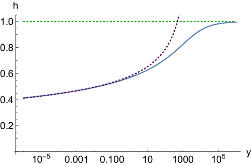
Here is the product logarithm function (also known as Lambert function),666 The product logarithm function is the inverse function of . In general, there exist infinite number of solutions for this equation, and and are the two real ones. In particular, is real for and is real for . Also, for large . A plot of and for small values of is shown in Fig. 4. This function is available ProductLog in Mathematica or special.lambertw in SciPy. See e.g., http://mathworld.wolfram.com/LambertW-Function.html. whose real branches are plotted in Fig. 4.
Eq. (39) expresses an equilibrium between the slope and the Hubble expansion which allows for efficient fragmentation: if the slope increases, in order to avoid the field acceleration, the friction due to cosmic expansion should compensate this effect. Alternatively, for , one can see Eq. (39) as a lower bound on that expresses, for given and , the necessary amount of fragmentation needed in order to slow down the field.
If Eq. (39) is satisfied, Eq. (38) has only one solution, with negative , which is given by777Before fragmentation is active, the field is only subject to its potential and to Hubble friction, and its equation of motion is simply , where we neglected a small oscillating term. This cannot be obtained as the limit of Eq. (40). The reason is that the equation of motion Eq. (38) was derived assuming fragmentation is active. In particular, we assumed . The acceleration is initially , and asymptotes to Eq. (40) as fragmentation starts.
| (40) |
Here and are dimensionless parameters which are defined as
| (41) |
Let us discuss the validity of the assumption Eq. (33). The effect of the axion fragmentaion in Eq. (38) has a exponential factor with a exponent . As we have discussed, for exponential particle production to occur, should be larger than 1. By using Eq. (40), we obtain
| (42) |
As we can see in Fig. 5, for fixed , is an monotonously increasing function of . For , as we will always assume, becomes small at , and is well approximated as . Thus, by requiring , we obtain
| (43) |
If , the LHS of Eq. (43) is positive and the inequality is satisfied. Thus, the above condition can be rewritten as
| (44) |
As long as Eq. (43) (or equivalently Eq. (44)) is satisfied, we can safely use given in Eq. (40). Note that is a monotonously increasing function of . Thus, we can see that Eq. (44) is satisfied for any if (and only if)
| (45) |
If this condition is satisfied, Eq. (40) for the acceleration can be used to describe the fragmentation process from its begininng until the end of that. In phenomenologically interesting applications , and Eq. (45) is always satisfied.
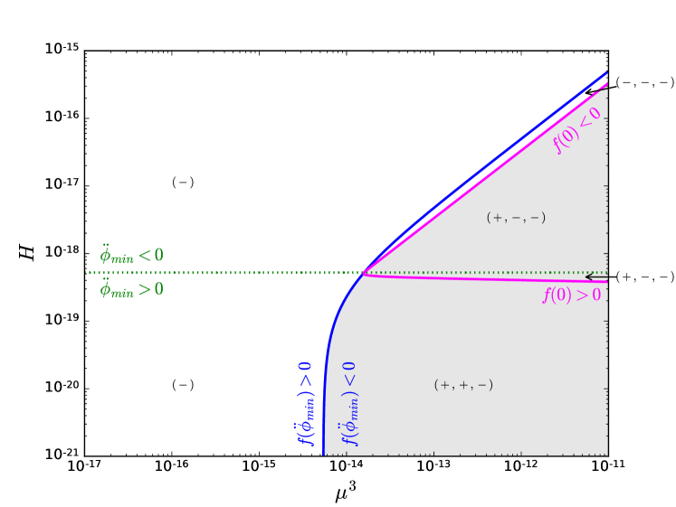
To summarize, in order for fragmentation to stop the rolling of the axion field we need to simultaneously impose the conditions of Eq. (26) and Eq. (39) to stop the axion. We are interested in the case in which the potential has local minima (i.e. ), and we will assume . In this case, Eq. (26) is trivially satisfied, and the only condition that must hold is Eq. (39).
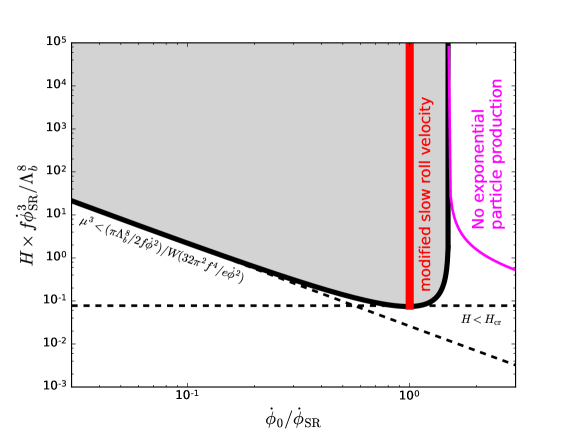
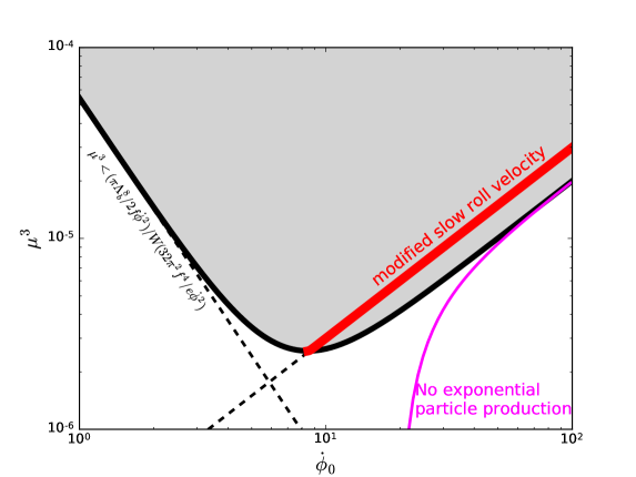
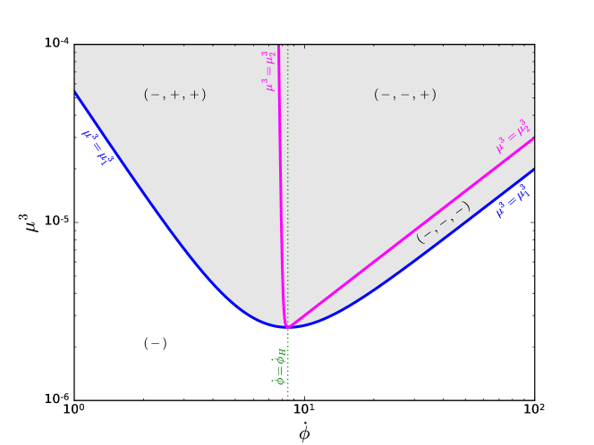
Figure 6 and Fig. 7 show examples of the parameter space in which Eq. (39) is satisfied. In the case of , there is an upperbound on because the acceleration effect by the slope should be weaker than the particle production effect. On the other hand, the bound on is very weak for and it becomes trivial for . Indeed, for , Eq. (39) is always satisfied, and the field is slowed down by Hubble friction without the need of fragmentation. In this region, the only bound comes from imposing that the exponential amplification of the fluctuations is active, as we do in Eq. (45).
It is interesting to investigate whether Eq. (38) admits constant velocity solutions. If such solutions exist the field can reach a steady state, and fragmentation can not stop the evolution. Equation (38) with has no solution for if (and only if):
| (46) |
is satisfied. This means that the axion zero mode cannot roll with constant velocity in such cases. For details, see the Appendix B.4. Note that Eq. (46) represents an upper bound on for fixed , but for fixed it can be rewritten as a lower bound on . On the other hand, for , Eq. (38) with admits solutions. To distinguish it from the slow roll velocity , we denote this velocity as the modified slow roll velocity . We show this velocity in red in Fig. 6 and Fig. 7. As long as , the modification to the slow roll velocity is small, i.e., .
3.2 Stopping conditions in several limits
In the previous section, we described the generic negative solution of and the stopping conditions. Here we discuss several cases in which the conditions can be simplified by taking some limits of the parameters.
3.2.1 and
First, let us discuss the limit of and . In this limit, Eqs. (25) and (39) are satisfied automatically. The expression for given in Eq. (40) is simplified to888 Eq. (47) can be obtained by separately taking the limits and of the two branches of Eq. (40), respectively, and using the expansions for and for , from which we get
| (47) |
This can be regarded as a refinement of Eq. (21). In this case, the amplification factor of the fluctuation energy in Eq. (35) is given by
| (48) |
In the derivation of Eq. (32) we assumed that , which is necessary for the validity of the low-energy EFT of the axion field, thus the amplification factor is much larger than , enhancing the efficiency of fragmentation. The time scale and the field excursion during the axion particle production are
| (49) | ||||
| (50) |
where we dropped subleading terms. The number of wiggles which the axion travels until it stops is
| (51) |
For example, for and , this number is .
3.2.2 and
Next, let us discuss the case in which and is small enough to be neglected. For , Eq. (39) can be simplified as
| (52) |
This corresponds to the left part of Figs. 6 and 7, which show how is irrelevant if . In the limit of , the negative solution Eq. (40) is simplified as
| (53) |
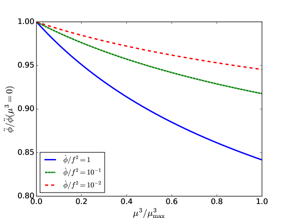
where are defined in Eq. (41). In the limit we recover Eq. (47). The acceleration monotonically decreases as a function of . In Fig. 8, we show the relative variation of when the slope goes from to defined in Eq. (52). As long as , the decrements of is at most %. Hence, the estimates for the fragmentation time and the total field excursion of Eqs. (49, 50) still provide a reliable approximation.
3.2.3
Let us discuss the case in which the initial velocity is equal to the slow roll velocity, i.e., . This is the case if the dynamics takes place during inflation, since the velocity is exponentially driven to the attractor slow-roll velocity irrespectively of the initial conditions. In this case, the condition Eq. (39) can be simplified to the following equation:
| (54) |
By replacing , the above condition Eq. (54) can be equivalently rewritten as a condition for and for given and :
| (55) |
This condition tells us that the Hubble friction is required to prevent acceleration in order to work the fragmentation mechanism if the slope is steeper than the threshold value . Alternatively, one can think of Eq. (54) as a lower bound on to have enough fragmentation to stop the field, for given and .
The negative solution Eq. (40) for is given as
| (56) |
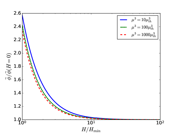
In Fig. 9, we show the ratio between evaluated with Eq. (56) and computed in Eq. (47) with , with the same velocity . Again, as long as Eq. (55) (or equivalently Eq. (54)) is satisfied, the acceleration is well described by the equation (47), thus the estimates for the fragmentation time and the total field excursion of Eqs. (49, 50) are reliable also in this case.
4 Numerical analysis of the equations of motion
In this section, we test the analytical understanding developed in Sec. 3 against a numerical solution of the equations of motion for the homogeneous mode , Eq. (9), and for the fluctuations , Eq. (10). We still limit ourselves to a linear level analysis, the validity of which will be further discussed in Sec. 5. For this calculation, we discretize the integral in Eq. (9) and take 10000 modes whose momentum is between and . The momenta are evenly spaced in logarithmic scale. The differential equations are solved numerically by the fourth order Runge-Kutta method.
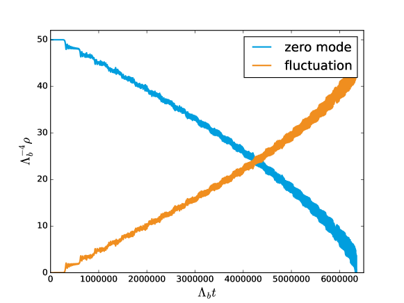
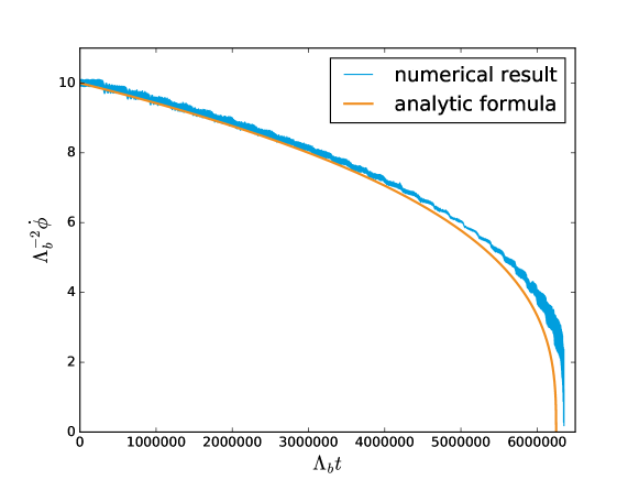
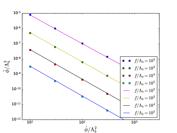
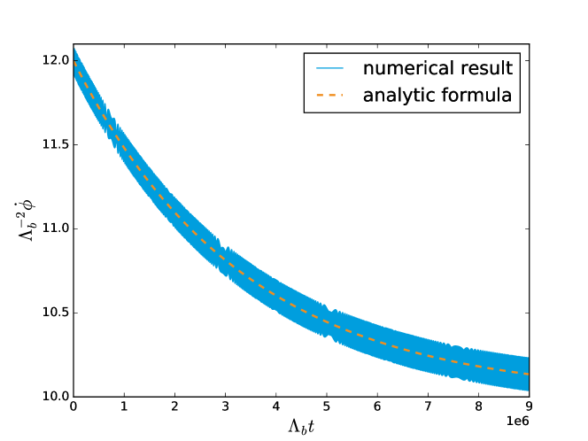
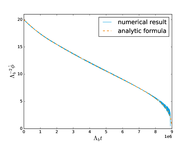
In Fig. 10, we show the time evolution of the energy of zero-mode and of the fluctuations, for and . The total energy is conserved and the figure shows that the energy of the zero-mode is successfully transferred to the fluctuations. In Figs. 11 and 12 we show the time evolution of and , again with and The numerical solution of Eqs. (9), (10) is compared to the result of Eq. (47). In Fig. 12, we show as a function of and , again comparing the numerical solution with the analytical results. Both Figs. 11 and 12 show that Eq. (47) is consistent with the direct numerical calculation with Eqs. (9, 10).
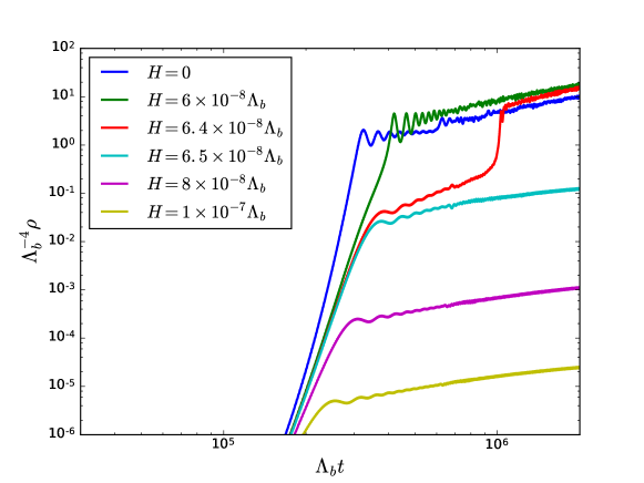
The effect of Hubble is shown in Fig. 13, where we plot the time evolution of the energy of fluctuations for several value of , with . As long as Eq. (54) is satisfied, Eq. (38) has only one solution and mildly depends on in this regime. However, when becomes larger than the critical value, the additional solutions given in Eqs. (144), (145) appear. Fig. 13 shows this transition behavior and the fragmentation process becomes slower for large value of .
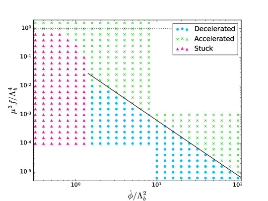
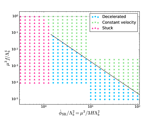
The phase diagrams of the axion particle production are shown in Figs. 14 and 15 for general values of and . In these figures, we take as the initial condition so that at the beginning. In Fig. 14, we take and show the parameter region in which the particle production is efficient in - plane. The figure shows that the condition Eq. (52) successfully reproduces the numerical result for the maximal slope that allows stopping due to fragmentation. In Fig. 15, we take nonzero and show the parameter region in which the particle production is efficient in the plane. The figure shows the excellent agreement between Eq. (54) and the numerical results.
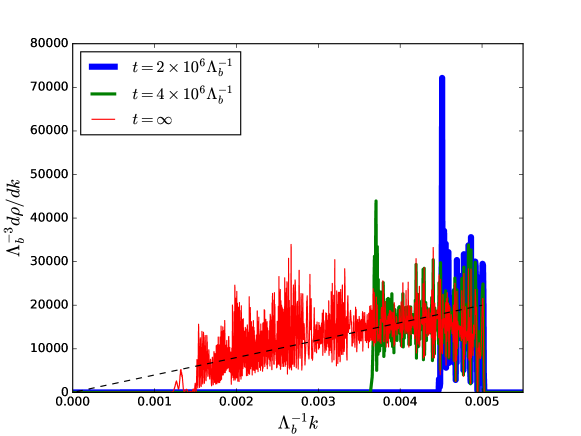
In Fig. 16, we show the time evolution of the energy spectrum of the fluctuations. This quantity can be easily estimated as follows. For and , by using Eqs. (32) and (47), we get
| (57) |
Then, we can calculate the energy spectrum after fragmentation as
| (58) |
where we dropped the oscillating terms. Fig. 16 shows that this estimation agrees with the result of the numerical calculation. From Eq. (58), we see that the peak frequency coincides with the initial position of the instability band, . Since , the emitted particles are typically relativistic. We expect that non-perturbative effects will broaden this spectrum (see the discussion in the next section).
5 Beyond the perturbative analysis
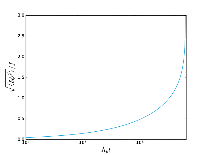
Let us comment on the validity of the leading order expansion of . For and , the size of fluctuation which is generated by the axion particle production can be estimated by using Eq. (57) as
| (59) |
where we averaged out the oscillating term in the integral. The time evolution of the ratio between and is shown in Fig. 17. We can see that at late times becomes large and we need to use non-perturbative methods for a concrete analysis in this regime. However, Fig. 17 shows that is satisfied during most of fragmentation process. Thus, we can expect that the estimation on the time scale Eq. (49) and field excursion Eq. (50) during fragmentation do not considerably vary from the ones obtained using a non-perturbative analysis, unless non-linear effects lead to a significant suppression of the growth of the field perturbations. This suppression is not expected to happen in our scenario due to the periodic potential, as we elaborate in the next paragraph.
A non-linear analysis would require a dedicated lattice study, on which we are currently working lattice . Preliminary results indicate that our main quantitative result, namely the estimate of the total field excursion before the axion is stopped Eq. (50), is correct up to a factor of order 1. The main difference that we expect to emerge from a non-linear analysis is the spectrum of excited fluctuations, which will be broadened by interactions among different modes. Moreover, the final field configuration will be inhomogeneous, with the scalar field populating more than one minima of the potential. This observation does not change significantly the picture we described so far, since the spread will always be much smaller compared to the total field excursion . Interestingly, formation of domain walls can occur in this scenario, depending on the non-linear evolution of the system and on other model dependent inputs such as the axion lifetime. We postpone this discussion to a future publication lattice .
A thorough comparison with other resonant systems is non-trivial, and it can hardly provide any insight on the non-linear behaviour of our model. Many models which were studied in the context of preheating feature a strong suppression of the growth at the non-linear level, generically due to the appearance of large effective mass terms. As an example, in Ref. Prokopec:1996rr , the resonant production of scalar particles from the oscillations of the inflaton is studied, and it is shown that both the perturbations of the inflaton field (which are generated non-linearly) and the inclusion of the quartic coupling , suppress the further growth of modes through a mass term (with appropriate coupling constants). Moreover, as fluctuations grow and drain energy from the zero-mode, the amplitude of the latter decreases, and hence the force driving the growth also progressively decreases. The case under study here has two peculiarities with respect to the one above. First, since the field traverses many periods of the periodic potential, the oscillating term that stimulates the growth of fluctuations has effectively a constant amplitude. Secondly, because of the approximate shift symmetry, no effective mass scale is generated in our case. Instead, all corrections enter the equation of motions only through the cosine potential, and thus there is no reason to expect any suppression. A setup similar to ours is discussed in Berges:2019dgr , in which a monodromy potential is studied. The paper shows that the evolution of the zero-mode stops shortly after the fluctuations have entered the non-linear regime, in accordance with our expectations.
6 Consequences: Relaxation of the electroweak scale
The axion fragmentation dynamics explored in this work should be taken into account in the evolution of any axion field which rolls down a wiggly potential. This phenomenon can fundamentally impact on a broad range of models, such as axion monodromy constructions and relaxion scenarios. In this section, we consider the effects of axion fragmentation on the relaxation mechanisms of the electroweak scale.
The relaxion mechanism is a solution to the electroweak hierarchy problem in which the Higgs mass term is controlled by the evolution of an axion-like field, the relaxion Graham:2015cka . This field evolves classically in the early universe until it stops close to a critical point, defined as the field value at which the Higgs VEV is zero. A key ingredient in this picture is a potential that features periodic wiggles, similar to the one discussed in this work. Relaxion fragmentation affects this construction in a substantial way Fonseca:2019lmc , as we detail below in the two main implementations of the relaxion idea which have been discussed in the literature so far.
Higgs dependent barriers
In the original proposal Graham:2015cka , the cosine term in the relaxion potential Eq. (1) has an amplitude dependent on the Higgs VEV, , with . For (QCD relaxion), where is the light quark masses. For the case with , the scale cannot be far from the electroweak scale, satisfying . The potential contains an interaction between the Higgs and the relaxion:
| (60) |
Initially, the Higgs mass term is positive, and the VEV is zero. As soon as , turns negative, a VEV develops, and the cosine term grows. In Ref. Graham:2015cka , it is assumed that the entire evolution takes place during a long period of inflation, and that Hubble friction is strong enough to stop the field as soon as the wiggles become larger than the average slope and the potential develop local minima, i.e. for . In particular, this happens when the time that it takes to roll over one period of the cosine term is longer than one Hubble time, i.e. for
| (61) |
Relaxion fragmentation offers an additional source of friction for the relaxion rolling. As discussed in Ref. Fonseca:2019lmc , this opens up two possibilities: on the one hand, the relaxion can be stopped by fragmentation even when Eq. (61) is not satisfied. On the other hand, it is possible to stop the relaxion field with a much shorter period of inflation or even in the absence of an inflationary background, with a negligible Hubble friction. This opens new possibilities for relaxion model building, independent from constraints on the inflationary sector. If relaxation takes place after inflation, it is possible, at least in principle, to conceive a model in which this phase has observable features, most probably in gravitational waves.This study could open the way to observable relaxion models.
Higgs independent barriers
An alternative relaxion construction was proposed in Hook:2016mqo , in which the amplitude of the cosine term is Higgs-independent, and the friction is mainly provided by gauge boson particle production. The relaxion couples to the Chern-Simons term of the massive SM boson, through a term
| (62) |
In the presence of this coupling, the equation of motion for the transverse polarization of the has a tachyonic instability for small mass
| (63) |
Contrarily to the case discussed above, initially the Higgs has a large VEV, and the SM particles are heavy. As the relaxion approaches the critical point and the gauge bosons become lighter, the tachyonic instability is triggered and the relaxion kinetic energy is dissipated through the production of bosons.
Fragmentation poses a serious threat to this model Fonseca:2019lmc . Since the amplitude of the cosine term is constant, fragmentation is always active, and the relaxion can be slowed down and stopped when the Higgs mass is large and close to the cut-off , thus spoiling the successful relaxation of the Higgs VEV to its current value. In particular,
-
•
if relaxation takes place after inflation Fonseca:2018xzp , the parameter space is restricted by the condition of avoiding excessive fragmentation. Moreover, once cosmological constraints are taken into account, the mechanism is excluded at least for a cutoff larger than few TeV.
-
•
If relaxation happens during inflation, the constraints from fragmentation reduce the available parameter space but do not exclude the model. The dark matter scenario discussed in Fonseca:2018kqf , in particular, is not affected.
7 Summary and outlook
In this paper, we discussed the production of quantum fluctuations during the evolution of an axion-like field rolling down a potential featuring wiggles, as given in Eq. (1). We refer to this effect as axion fragmentation. While the production of quanta is suppressed when an axion oscillates around the minimum of its potential, unless the initial amplitude is very large and the initial position of the field is tuned close to the maximum of the sinusoidal potential, the effect is very large in the case where the axion field crosses many of its maxima. We studied in detail under which conditions axion fragmentation can efficiently stop the evolution of the field. We computed the time scale needed for stopping and the corresponding field excursion.
The wavefunction of the fluctuations obeys the Mathieu equation and the energy of the modes within the instability band Eq. (12) grows exponentially. If both the slope of the potential and the Hubble expansion rate are sufficiently small, this particle production effect decelerates the homogeneous mode. The condition is given as Eq. (26) and Eq. (39) in terms of the initial field velocity, the linear slope of the potential, the Hubble rate, the size of the barriers and the periodicity of the sinusoidal potential. The corresponding acceleration is given in Eq. (40).
Axion fragmentation is a generic effect which can have interesting phenomenological implications. It is particularly relevant for the mechanism of cosmological relaxation of the electroweak scale. We dedicate a separate paper to study in details these implications in Ref. Fonseca:2019lmc , where we conclude that new regions of parameter space open and novel directions for relaxion model building are offered by this effect.
In the present work we study the regime in which the potential has local minima, see Eq. (2). It would be interesting to investigate the effect of fragmentation in the case in which the oscillating term in potential does not generate local minima. This may have implications for some relaxion models where loop effects generate small Higgs-independent barriers, so that there are constant wiggles with small amplitude during the whole scanning of the Higgs mass parameter.
Another promising direction will be to explore the impact of axion quanta on the cosmological history of the universe. As discussed in Ref. Fonseca:2019lmc , depending on the equation of the state of the universe during axion rolling, the produced quanta may represent a significant fraction of the energy density of the universe. Whether they can be viable dark matter candidates, depends on the time of fragmentation. Such quanta may in turn induce gravitational waves. They may be diluted or leave observable imprints. These effects deserve detailed studies which we postpone for future work.
Acknowledgements
The authors thank Yohei Ema, Hyungjin Kim, Kyohei Mukaida, and Gilad Perez, Alexander Westphal for useful discussions. We are grateful to Sven Krippendorf for important discussions in the initial stages of this work. This work is supported by the Deutsche Forschungsgemeinschaft under Germany’s Excellence Strategy - EXC 2121 “Quantum Universe” - 390833306. Research in Mainz is supported by the Cluster of Excellence “Precision Physics, Fundamental Interactions, and Structure of Matter” (PRISMA+ EXC 2118/1) funded by the German Research Foundation(DFG) within the German Excellence Strategy (Project ID 39083149).
Appendix A Approximate solution of Eq. (10)
Let us discuss the evolution of the wave functions . The boundary condition at is given by Eq. (6). For the duration of the amplification process, we can neglect the Hubble friction term in the equation of motion. This is justified for if is satisfied (see the discussion around Eq. (25)). The mode function satisfies the following equation of motion:
| (64) |
Note that the Hubble expansion still has its effect via term although we have dropped .
A.1 and (Mathieu equation)
First, let us consider the case of constant and as in Sec. 2. Taking the scale factor , Eq. (64) is simplified as
| (65) |
This is the Mathieu equation, and it is known that grows exponentially when satisfies
| (66) |
Let us see this behavior explicitly. We define and for convenience:
| (67) |
Then, Eq. (65) is rewritten as
| (68) |
We assume and we will expand perturbatively in . On the other hand, we assume , as we are interested in the first instability band. In the limit , the solution is of the form for constant and . This motivates the following ansatz for :
| (69) |
Here and encode the rapid oscillations of the solution, while ’s and ’s are slowly varying coefficients. The terms with are introduced to maintain a consistency with Eq. (68). We define a dimensionless time :
| (70) |
By plugging Eqs. (69, 70) into Eq. (65), we obtain the following differential equations for ’s and ’s:
| (71) | ||||
| (72) |
for and, for ,
| (73) | ||||
| (74) |
The differential equations above indicate a simple hierarchy between the coefficients
| (75) |
At the leading order in , we can neglect and with , and also the second derivative in Eqs. (71), (72). We obtain
| (76) | ||||
| (77) |
For , the asymptotic behavior of and are then
| (78) |
For the solution is unstable. On the contrary, for it oscillates as .
A.2 Small non-zero and
Let us now introduce a small, constant acceleration :
| (79) |
where . The assumption of neglecting higher derivatives is justified in the main text, see the discussion around Eq. (30). Let us consider a given mode . By a simple time shift, here we define as the time at which is at the center of the instability band, which is now defined as
| (80) |
As the velocity decreases, the instability band moves to lower modes. For a given , we will solve the equations of motion from a time slightly before it enters the instability band, until slightly after it exits, and we will see how the initial oscillatory behaviour is then amplified inside the instability band until the mode exits. We assume for an ansatz similar to Eq. (69), but this time the cosine will depend on :
| (81) |
Again, we only consider the case in which the velocity is larger than the wiggles, . In order to keep the evolution under perturbative control, we assume that the time spend in the instability band is short, and that the velocity changes only slightly during this time. Furthermore, we assume that the effect of Hubble friction is small:
| (82) |
In Eq. (81) we make explicit the dependence of the mode functions on the scale factor. When taking the derivatives , we will keep this factor as a constant, consistently with the assumption that the amplification time for any mode is much shorter than a Hubble time. By plugging the above into the equation of motion Eq. (64), we obtain the equations for the coefficients of the sine and cosine terms. Similarly to before, the equations show an hierarchy . This can be extracted from the equations of motion or by analogy with the constant velocity case, remembering that the acceleration gives only a small correction to the evolution according to Eq. (82). Thus, we can neglect the contribution from the terms. For we obtain the equation for the coefficients of and :
| (83) | ||||
| (84) |
By using the results in the previous section, we can estimate that . Thus, by assuming , we can drop and in the above equations. We require the time evolution of is sufficiently slower than that of and , i.e., . This condition can be understood as follows. The time evolution of the energy of zero mode is given by . The energy stored in the fluctuations inside the instability band is
| (85) |
Thus, dropping second time derivatives, the growth of is given by
| (86) |
The growth in energy of the modes inside the instability band correspond to the slow-down of the zero mode. Thus, , and we obtain . Due to the smallness of the band width , , and hence . The last condition can be rewritten as
| (87) |
which implies . Thus, we can drop the terms and . Finally, we define the auxiliary quantities
| (88) |
where . Furthermore, since we assume the Hubble expansion rate is sufficiently small as explained in Eq. (82), we expand the scale factor as . In terms of and , we obtain
| (89) | ||||
| (90) |
A.2.1 Generic solution for Eqs. (89, 90)
Let us discuss the solution of Eqs. (89, 90) for . Eqs. (89, 90) can be rewritten as
| (91) | |||
| (92) |
In the case of , we can use WKB approximation for these differential equations. can be written as where and . At leading and next to leading order in , we obtain the following equations from Eq. (91):
| (93) | ||||
| (94) |
Solutions of the above equation are
| (95) | |||
| (96) |
Similarly, by plugging into Eq. (92), we obtain
| (97) | |||
| (98) |
The generic solution for is given as
| (99) | ||||
| (100) |
For ,
| (101) | ||||
| (102) |
For ,
| (103) | ||||
| (104) |
In Eqs. (99-102), , , and are constants, and the relative factors between and are determined to satisfy Eqs. (89, 90).
The WKB approximation fails for , as can be seen for example from the last term in Eq. (94) becoming of order . For , Eqs. (89, 90) can be approximated as
| (105) | |||
| (106) |
Eq. (106) can be rewritten as an Airy/Stokes equation, the solution of which can be written in terms of the Airy functions , as
| (107) |
where and are constants. can be obtained using Eq. (105):
| (108) |
Here and . Similarly, we obtain the generic solution for :
| (109) | ||||
| (110) |
where and are constants.
Now we have the generic solution of Eqs. (89, 90) in the following five separate region of :
- •
- •
- •
- •
- •
To connect each region of , we will need the asymptotic form of Airy functions:
| (111) |
and
| (112) |
We will also need the expansion of the phases of the WKB solutions close to the critical points :
| (113) | ||||
| (114) | ||||
| (115) | ||||
| (116) |
A.2.2 Matching with the initial condition Eq. (6)
The solutions described have free coefficients that can be obtained from matching at the intersection of their regime of validity and with the initial condition
| (117) |
where Eq. (117) is specified up to a phase, which we choose in order to make the phases of and real and positive for . The initial conditions for and are given as
| (118) |
where is a phase which we do not specify here.
Matching Eqs. (99, 100) with the initial condition Eq. (118) at , we have
| (119) | ||||
| (120) |
For , can be written as a linear combination of Airy functions. The solution which is consistent with Eqs. (119, 120) is
| (121) | ||||
| (122) |
For , we can use WKB approximation again. The solution consistent with Eqs. (121, 122) is given as
| (123) | ||||
| (124) |
Here we dropped exponentially suppressed term . For , can be written as a linear combination of Airy functions. Matching onto Eq. (123, 124) gives
| (125) | ||||
| (126) |
Finally, for , we can use WKB approximation again. Matching with Eqs. (125, 126) gives
| (127) | ||||
| (128) |
Therefore, after amplification has ended, the asymptotic behavior of is
| (129) |
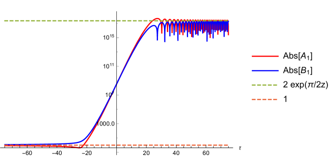
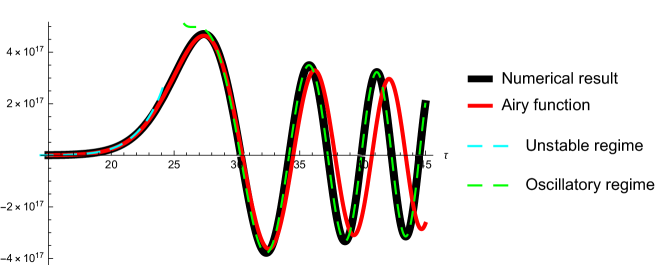
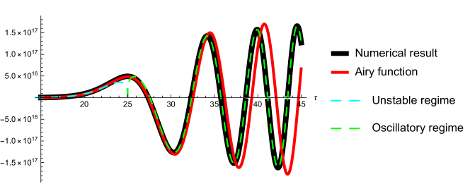
Figure 18 shows the good agreement of a numerical solution of Eqs. (89, 90) with the analytic formulae above. By using the definition of given in Eq. (88), we obtain Eq. (32).
So far, we have discussed the case with , i.e., . In closing this section, let us briefly look at the solutions of Eqs. (89, 90) for , i.e., . This solution is required to discuss positive solution and solution in Eq. (38). For , the initial conditions for and is
| (130) |
Eq. (89, 90) are symmetric under the transformation of and . Also, complex conjugation is a symmetry of the equation of motion. The initial conditions in Eq. (130) can be obtained by taking complex conjugate of Eq. (118) after exchanging . Thus, and for can be obtained from Eqs. (119–128) by replacing and
| (131) |
The coefficients , for are given as
| (132) | ||||
| (133) |
and for are given as
| (134) | ||||
| (135) |
Therefore, after amplification has ended, the asymptotic behavior of is
| (136) |
By using the definition of given in Eq. (88), we obtain Eq. (32).
Appendix B Detailed analysis on Eq. (38)
In this section, we discuss Eq. (38) in detail.
B.1 The solutions of Eq. (38)
Let us discuss the solutions of Eq. (38), which we report here for simplicity:
| (137) |
By defining
| (138) |
Eq. (38) can be rewritten as
| (139) |
where and are dimensionless parameters which are defined as
| (140) |
Eq. (139) can be rewritten as
| (141) |
which has the following solutions:
| (142) |
where , are the two main branches of the Lambert function (product logarithm). The first two solutions have , the other two have . Formally, the first solution only exists for . By using the consistency condition of EFT, we can assume , i.e., . In terms of the acceleration , the analytic solutions of Eq. (137) are given as
| (143) | ||||
| (144) | ||||
| (145) |
Again, and exist only if . Moreover, , and if they exist. The solution has two different rappresentations for positive or negative , but it is continuous in at when diverges. Finally, by looking at Eq. (137), one notices that , as it is expected since the particle production effect always takes away energy from the zero mode.
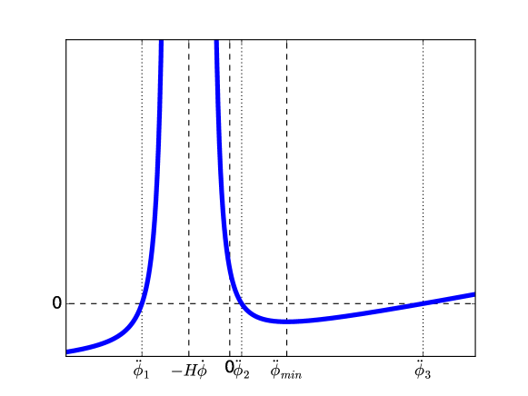
B.2 The condition not to have positive solution
In order to stop the axion rolling, the acceleration should always be negative. Before fragmentation starts, the field is only subject to the slope and Hubble friction, . Let us start by deriving a condition not to have a solution . Let us define as
| (146) |
Eq. (38) is equivalent to . We can easily see the following property of :
| (147) | ||||
| (148) | ||||
| (149) | ||||
| (150) | ||||
| (151) | ||||
| (152) |
The function monotonously increases for because of . There exists one local minimum at . A typical behavior of is shown in Fig. 19. The solutions of are classified depending on the sign of , , and , which are given as
| (153) | ||||
| (154) | ||||
| (155) |
After having discussed the behaviour of the function , it is clear that the equation has up to three solutions, which correspond to , , of Eqs. (143-145). These are summarized in Tab. 1. We are interested in a situation in which the field is slown-down by fragmentation, thus we want to avoid solutions with . This condition, depending on the sign of , can be written as
| (156) | ||||
| (157) |
Eqauations (156, 157) cover, respectively, a situation in which the solution do not exist and one in which they do exist but they are negative. It is convenient to rewrite this condition as an upperbound on :
| (158) |
where we have defined
| (159) | ||||
| (160) | ||||
| (161) |
Note that corresponds to , corresponds to , and corresponds to . Moreover, for . Figure 20 shows the parameter region which is excluded by the condition Eq. (158). is a monotonously decreasing function of ; thus, Eq. (158) are equivalent to
| (162) |
Here is defined as the solution of , so that is equivalent to , and it is explicitly written as
| (163) |
where satisfies
| (164) |
The numerical value of is shown in Fig. 21.
| ( do not exist.) | |
|---|---|
| , | |
| , , | |
| , , |
B.3 The stopping condition
Before fragmentation is active, . This is not a solution of Eq. (137), and does not result as the limit of . The failure of to reproduce this initial condition is due to our assumption Eq. (87), which gives a minimal value of (and thus a minimal efficiency of the fragmentation effect) below which our calculation is not reliable. Still, in this regime, we can assume that varies continuously. When fragmentation turns on and Eq. (137) becomes valid, will smoothly decrease from its initial value until it reaches one of the solutions in Eqs. (143-145), and it will stick to it for the rest of the evolution. In order to understand the behaviour during this phase, it is also useful to notice that, if , will decrease. Oppositely, if , will increase. Hence, is a stable solution, as well as (if it exists). On the contrary, , if it exists, is an unstable solution.
Let us now discuss the necessary and sufficient conditions in order to guarantee that the field slows-down until it stops. The conditions in Eqs. (156, 157), or equivalently in Eq. (162), give a bound on the slope that depends on the velocity . If this condition is satisfied for , initially the solutions to Eq. (137) have :
| (165) |
This is a necessary but not sufficient condition to stop the rolling of the field . Indeed, should be negative until the axion will be stopped. In the case , the only solution of is . Thus, at the beginning, becomes and starts to decrease. As decreases, changes continuously and is always satisfied even if or solution appear at some velocity . As we have seen in App. B.1, is always negative and the field will be stopped in the end.
On the other hand, in the case , has three solutions. The acceleration decreases from the initial value until it reaches , because . Following the discussion in Sec. B.2, the solution exists and is negative if both and are satisfied. In this case, the field starts to decelerate. As decreases, changes continuously and is always satisfied. However, is not always negative, and in particular, , since, as we discussed below the definitions Eqs. (159, 160, 161), for , and .999 Alternatively, by using the definition Eqs. (159, 160, 161), one can show that takes its minimum at , and then, . Also, we can show . Thus, holds and for is positive. This is depicted in Fig. 22, which shows that for and coincide, leaving space only for positive . This means that there exists a velocity such that for . (For an existence condition of solution, see also the Appendix B.4.) If the axion evolution is governed by the solution , the field will approach that constant velocity, and its rolling cannot be stopped. Thus, in order to stop the axion rolling, we need to assume that the solutions do not exist, i.e., that
| (166) |
To conclude this section, let us show a numerical example that supports the analytical discussion above. In Fig. 23, we show , , and as a function of . We take , , and in units of . In this example, at the beginning of fragmentation becomes if , and if . In Fig. 24, we show the time evolution of for and . The numerical result is consistent with for , and for , confirming our understanding.

B.4 Modified slow roll velocity
In this section, we want to determine the existence conditions and the value of a constant-velocity solution of the equation of motion, under the effect of fragmentation. Fragmentation acts as an additional source friction, thus it is clear that this velocity, which we call , will be smaller than the usual slow-roll velocity . As we discussed in App. B.3, if such a solution exists the field will decelerate until it reaches , and its evolution cannot be stopped.
First, let us discuss the existence condition of the solution of . Let us define . Then, we can rewrite as
| (167) |
For given , , and , there exists a critical value of the Hubble expansion rate , such that has two solution if , one solution if , and no solution if . In order to avoid constant velocity solutions, we need to impose . It should be noticed that this condion is an upper bound on if is fixed, but it can be rewritten as a lower bound on for fixed . If , should not have solution tostop the axion. For the consistency of the EFT description we assume that . Thus, we can treat as a small parameter. In this case, the solution of Eq. (167) with is close to 1, since we expect the deviations from the slow roll velocity to be at least of order . Equation Eq. (167) can then be expressed as
| (168) |
where, after simplifying a factor , we expanded separately the right-hand side and the exponent of the left-hand side for . This procedure is justified by the observation that the exponent is very large and thus the LHS changes much more rapidly than the RHS with . By solving and simultaneously, we obtain
| (169) |
For , Eq. (167) admits two solutions. The smallest of the two has and is unstable. The largest solution is instead stable, and can be regarded the modified slow roll velocity, given by
| (170) |
References
- (1) P. Svrcek and E. Witten, Axions In String Theory, JHEP 06 (2006) 051 [hep-th/0605206].
- (2) A. Arvanitaki, S. Dimopoulos, S. Dubovsky, N. Kaloper and J. March-Russell, String Axiverse, Phys. Rev. D81 (2010) 123530 [0905.4720].
- (3) J. Preskill, M. B. Wise and F. Wilczek, Cosmology of the Invisible Axion, Phys. Lett. 120B (1983) 127.
- (4) L. F. Abbott and P. Sikivie, A Cosmological Bound on the Invisible Axion, Phys. Lett. 120B (1983) 133.
- (5) M. Dine and W. Fischler, The Not So Harmless Axion, Phys. Lett. 120B (1983) 137.
- (6) E. Pajer and M. Peloso, A review of Axion Inflation in the era of Planck, Class. Quant. Grav. 30 (2013) 214002 [1305.3557].
- (7) P. Adshead, J. T. Giblin, T. R. Scully and E. I. Sfakianakis, Gauge-preheating and the end of axion inflation, JCAP 1512 (2015) 034 [1502.06506].
- (8) V. Domcke, Y. Ema and K. Mukaida, Chiral Anomaly, Schwinger Effect, Euler-Heisenberg Lagrangian, and application to axion inflation, 1910.01205.
- (9) P. Adshead, J. T. Giblin, M. Pieroni and Z. J. Weiner, Constraining axion inflation with gravitational waves from preheating, 1909.12842.
- (10) G. Servant, Baryogenesis from Strong Violation and the QCD Axion, Phys. Rev. Lett. 113 (2014) 171803 [1407.0030].
- (11) V. Domcke, B. von Harling, E. Morgante and K. Mukaida, Baryogenesis from axion inflation, JCAP 1910 (2019) 032 [1905.13318].
- (12) F. Wilczek, Problem of Strong and Invariance in the Presence of Instantons, Phys. Rev. Lett. 40 (1978) 279.
- (13) R. D. Peccei and H. R. Quinn, CP Conservation in the Presence of Instantons, Phys. Rev. Lett. 38 (1977) 1440.
- (14) D. J. E. Marsh, Axion Cosmology, Phys. Rept. 643 (2016) 1 [1510.07633].
- (15) I. G. Irastorza and J. Redondo, New experimental approaches in the search for axion-like particles, Prog. Part. Nucl. Phys. 102 (2018) 89 [1801.08127].
- (16) P. B. Greene, L. Kofman and A. A. Starobinsky, Sine-Gordon parametric resonance, Nucl. Phys. B543 (1999) 423 [hep-ph/9808477].
- (17) A. Arvanitaki, S. Dimopoulos, M. Galanis, L. Lehner, J. O. Thompson and K. Van Tilburg, The Large-Misalignment Mechanism for the Formation of Compact Axion Structures: Signatures from the QCD Axion to Fuzzy Dark Matter, 1909.11665.
- (18) R. T. Co, E. Gonzalez and K. Harigaya, Axion Misalignment Driven to the Hilltop, JHEP 05 (2019) 163 [1812.11192].
- (19) B. Freivogel, Anthropic Explanation of the Dark Matter Abundance, JCAP 1003 (2010) 021 [0810.0703].
- (20) P. W. Graham, D. E. Kaplan and S. Rajendran, Cosmological Relaxation of the Electroweak Scale, Phys. Rev. Lett. 115 (2015) 221801 [1504.07551].
- (21) L. McAllister, E. Silverstein and A. Westphal, Gravity Waves and Linear Inflation from Axion Monodromy, Phys. Rev. D82 (2010) 046003 [0808.0706].
- (22) R. Flauger, L. McAllister, E. Pajer, A. Westphal and G. Xu, Oscillations in the CMB from Axion Monodromy Inflation, JCAP 1006 (2010) 009 [0907.2916].
- (23) J. Jaeckel, V. M. Mehta and L. T. Witkowski, Monodromy Dark Matter, JCAP 1701 (2017) 036 [1605.01367].
- (24) J. Berges, A. Chatrchyan and J. Jaeckel, Foamy Dark Matter from Monodromies, JCAP 1908 (2019) 020 [1903.03116].
- (25) M. P. Hertzberg, Quantum Radiation of Oscillons, Phys. Rev. D82 (2010) 045022 [1003.3459].
- (26) M. A. Amin, Inflaton fragmentation: Emergence of pseudo-stable inflaton lumps (oscillons) after inflation, 1006.3075.
- (27) M. A. Amin, R. Easther and H. Finkel, Inflaton Fragmentation and Oscillon Formation in Three Dimensions, JCAP 1012 (2010) 001 [1009.2505].
- (28) S. Antusch, F. Cefala, S. Krippendorf, F. Muia, S. Orani and F. Quevedo, Oscillons from String Moduli, JHEP 01 (2018) 083 [1708.08922].
- (29) J. Ollé, O. Pujolàs and F. Rompineve, Oscillons and Dark Matter, 1906.06352.
- (30) A. D. Dolgov and D. P. Kirilova, ON PARTICLE CREATION BY A TIME DEPENDENT SCALAR FIELD, Sov. J. Nucl. Phys. 51 (1990) 172.
- (31) J. H. Traschen and R. H. Brandenberger, Particle Production During Out-of-equilibrium Phase Transitions, Phys. Rev. D42 (1990) 2491.
- (32) L. Kofman, A. D. Linde and A. A. Starobinsky, Reheating after inflation, Phys. Rev. Lett. 73 (1994) 3195 [hep-th/9405187].
- (33) Y. Shtanov, J. H. Traschen and R. H. Brandenberger, Universe reheating after inflation, Phys. Rev. D51 (1995) 5438 [hep-ph/9407247].
- (34) L. Kofman, A. D. Linde and A. A. Starobinsky, Towards the theory of reheating after inflation, Phys. Rev. D56 (1997) 3258 [hep-ph/9704452].
- (35) A. Hook and G. Marques-Tavares, Relaxation from particle production, JHEP 12 (2016) 101 [1607.01786].
- (36) K. Choi, H. Kim and T. Sekiguchi, Dynamics of the cosmological relaxation after reheating, Phys. Rev. D95 (2017) 075008 [1611.08569].
- (37) W. Tangarife, K. Tobioka, L. Ubaldi and T. Volansky, Dynamics of Relaxed Inflation, JHEP 02 (2018) 084 [1706.03072].
- (38) O. Matsedonskyi and M. Montull, Light Higgs Boson from a Pole Attractor, Phys. Rev. D98 (2018) 015026 [1709.09090].
- (39) N. Fonseca, E. Morgante and G. Servant, Higgs relaxation after inflation, JHEP 10 (2018) 020 [1805.04543].
- (40) N. Fonseca and E. Morgante, Relaxion Dark Matter, Phys. Rev. D100 (2019) 055010 [1809.04534].
- (41) M. Ibe, Y. Shoji and M. Suzuki, Fast-Rolling Relaxion, JHEP 11 (2019) 140 [1904.02545].
- (42) S.-J. Wang, Paper-boat relaxion, Phys. Rev. D99 (2019) 095026 [1811.06520].
- (43) K. Kadota, U. Min, M. Son and F. Ye, Cosmological Relaxation from Dark Fermion Production, 1909.07706.
- (44) N. Fonseca, E. Morgante, R. Sato and G. Servant, Relaxion Fluctuations (Self-stopping Relaxion) and Overview of Relaxion Stopping Mechanisms, 1911.08473.
- (45) N. McLachlan, Theory and Applications of Mathieu Functions. Oxford Univ. Press, Clarendon, 1947.
- (46) I. Kovacic, R. Rand and S. M. Sah, Mathieu’s equation and its generalizations: Overview of stability charts and their features, Applied Mechanics Reviews 70 (2018) 020802.
- (47) E. Morgante and R. Sato, Lattice analysis of relaxion fragmentation and its cosmological consequences, in preparation, .
- (48) T. Prokopec and T. G. Roos, Lattice study of classical inflaton decay, Phys. Rev. D55 (1997) 3768 [hep-ph/9610400].