Time-varying constrained proximal type dynamics
in multi-agent network games

Abstract

In this paper, we study multi-agent network games subject to affine time-varying coupling constraints and a time-varying communication network. We focus on the class of games adopting proximal dynamics and study their convergence to a persistent equilibrium. The assumptions considered to solve the problem are discussed and motivated. We develop an iterative equilibrium seeking algorithm, using only local information, that converges to a special class of game equilibria. Its derivation is motivated by several examples, showing that the original game dynamics fail to converge. Finally, we apply the designed algorithm to solve a constrained consensus problem, validating the theoretical results.

I Introduction

I-A Motivation: Multi-agent decision making over networks

In multi-agent decision making over networks, all the decision makers, in short, agents, share their information only with a selected number of agents. In particular, the agents’ state (or decision) is the result of a local decision making process, e.g. a constrained optimization problem, and a distributed communication with the neighboring agents, defined by the communication network. In many problems, the goal of the agents is reaching a collective equilibrium state, where no agent can benefit from changing its state. The local interation between the agents is exploited in opinion dynamics to model the evolution of a population’s collective opinion as an emerging phenomenon of the local interactions, see [1, 2, 3]. Another interesting consequence of the communication structure is that the agents keep their own data private, exchanging information only with selected agents. This characteristic is of particular interest in, for example, traffic and information networks problems [4] or in the charging scheduling of electric vehicles [5, 6]. This class of problems arises also in other applications, e.g., in smart grids [7, 8] and sensor network [9], [10].

I-B Literature overview: Multi-agent optimization and multi-agent network games

In this work, we study a particular instance of the problem introduced above, namely a multi-agent network game, where the communication network and the constraints between the agents are both time-varying. Multi-agent network games arise from the well established field of distributed optimization and equilibrium seeking over networks. In the past years, several results were proposed for optimization problems subject to a time-varying communication network: in [11] the subgradients of the cost functions are bounded and the communication is described by a strongly connected sequence of directed graphs, while in [12] the cost functions are assumed to be continuously differentiable and a linearly convergent algorithm is designed under the assumption of a time-varying undirected communication network. Another approach, explored in [13], is to construct a game, whose emerging behavior solves the optimization problems. In this case, the cost functions are differentiable and the communication ruled by an undirected time-varying graph connected over time.

The problem of noncooperative multi-agent games, subject to coupling constrains, was firstly studied in [14], under the assummptions of continuosly differentiable cost functions and no network structure between the agents. In the past years, several researchers focused on this class of problems providing many results for games over networks, e.g., in [15, 16, 5] where the communication network is always assumed undirected, while the cost functions are chosen either differentiable or continuously differentiable. Moreover, some authors also focused on the class of noncooperative games over time-varying communication network, in particular on the unconstrained case. For example, in [17] differentiable and strictly convex cost functions with Lipschitz continuous gradient were considered, where the sequence of time-varying communication networks was repeatedly strongly connected, and the associated adjacency matrices doubly stochastic.

I-C Paper contribution

A complete formulation of multi-agent network games, subject to proximal type dynamics, can be found in [8] where the unconstrained case is studied for a time-varying strongly connected communication network, described by a doubly stochastic adjacency matrix. In [18, 19], the condition on the double stochasticity of the adjacency matrix was relaxed, in the first case by means of a dwell time. Notice that these types of games can also be rephrased as paracontracions; in this framework, the work in [20] provided convergence for repeatedly jointly connected digraphs. Iterative equilibrium seeking algorithms were developed for constrained multi-agent network games in [8, 19] under the assumption of a static communication network.

In this work, we aim to address the problem of a constrained multi-agent network games subject to a time-varying communication network. In particular, we first discuss the convergence of the game and motivate the technical assumption needed to ensure the existence of an equilibrium, and then we develop an equilibrium seeking algorithm that achieves global convergence for the game at hand. The main difference with the work in [19] is the presence of both time-varying communication network and time-varying constraints, and this generalization leads to several technical challenges, requiring a more involved convergence analysis.

II NOTATION

II-A Basic notation

The set of real, positive, and non-negative numbers are denoted by $\mathbb{R}$, $\mathbb{R}_{>0}$ and $\mathbb{R}_{\geq 0}$, respectively; $\overline{\mathbb{R}}:=\mathbb{R}\cup\{\infty\}$. The set of natural numbers is denoted by $\mathbb{N}$. For a square matrix $A\in{\mathbb{R}}^{n\times n}$, its transpose is denoted by $A^{\top}$, $[A]_{i}$ denotes the $i$-th row of the matrix, and $[A]_{ij}$ the element in the $i$-th row and $j$-th column.Also, $A\succ 0$ ($A\succeq 0$) stands for a symmetric and positive definite (semidefinite) matrix, while $>$ ($\geq$) describes an element wise inequality. $A\otimes B$ is the Kronecker product of the matrices $A$ and $B$. The identity matrix is denoted by $I_{n}\in{\mathbb{R}}^{n\times n}$, and $\boldsymbol{0}$ ($\boldsymbol{1}$) represents the vector/matrix with only $0$ ($1$) elements. For $x_{1},\dots,x_{N}\in\mathbb{R}^{n}$ and $\mathcal{N}=\{1,\dots,N\}$, the collective vector is denoted as $\boldsymbol{x}:=\mathrm{col}((x_{i})_{i\in\mathcal{N}})=[x_{1}^{\top},\dots,x_{N}^{\top}]^{\top}$ and $\boldsymbol{x}_{-i}:=\mathrm{col}((x_{j})_{j\in\mathcal{N}\setminus\{i\}})=[x_{1}^{\top},\dots,x_{i-1}^{\top},x_{i+1}^{\top},\dots,x_{N}^{\top}]^{\top}$. Given the $N$ operators $A_{1},\dots,A_{N}$, ${\mathrm{diag}}(A_{1},\dots,A_{N})$ denotes a block-diagonal operators with $A_{1},\dots,A_{N}$ as diagonal elements. The Cartesian product of the sets $\Omega_{1},\dots,\Omega_{N}$ is described by $\prod^{N}_{i=1}\Omega_{i}$. Given two vectors $x,y\in{\mathbb{R}}^{n}$ and a symmetric and positive definite matrix $Q\succ 0$, the weighted inner product and norm are denoted by $\langle\,x\,|\,y\,\rangle_{Q}$ and $\lVert x\rVert_{Q}$, respectively; the $Q-$induced matrix norm is denoted by $\lVert A\rVert_{Q}$. A real $n$ dimensional Hilbert space obtained by endowing $\mathcal{H}=({\mathbb{R}}^{n},\lVert\,\cdot\,\rVert)$ with the product $\langle\,x\,|\,y\,\rangle_{Q}$ is denoted by $\mathcal{H}_{Q}$.

II-B Operator-theoretic notations and definitions

The identity operator is defined by $\textrm{Id}(\cdot)$. The indicator function $\iota_{\mathcal{C}}:{\mathbb{R}}^{n}\rightarrow[0,+\infty]$ of $\mathcal{C}\subseteq{\mathbb{R}}^{n}$ is defined as $\iota_{\mathcal{C}}(x)=0$ if $x\in\mathcal{C}$; $+\infty$ otherwise. The set valued mapping $N_{\mathcal{C}}:{\mathbb{R}}^{n}\rightrightarrows{\mathbb{R}}^{n}$ stands for the normal cone to the set $\mathcal{C}\subseteq{\mathbb{R}}^{n}$, that is $N_{\mathcal{C}}(x)=\{u\in{\mathbb{R}}^{n}\,|\,\mathrm{sup}\langle\mathcal{C}-x,u\rangle\leq 0\}$ if $x\in\mathcal{C}$ and $\varnothing$ otherwise. The graph of a set valued mapping $\mathcal{A}:\mathcal{X}\rightrightarrows\mathcal{Y}$ is $\mathrm{gra}(\mathcal{A}):=\{(x,u)\in\mathcal{X}\times\mathcal{Y}\,|\,u\in\mathcal{A}(x)\}$. For a function $\phi:{\mathbb{R}}^{n}\rightarrow\overline{\mathbb{R}}$, define $\mathrm{dom}(\phi):=\{x\in{\mathbb{R}}^{n}|f(x)<+\infty\}$ and its subdifferential set-valued mapping, $\partial\phi:\mathrm{dom}(\phi)\rightrightarrows{\mathbb{R}}^{n}$, $\partial\phi(x):=\{u\in{\mathbb{R}}^{n}|\>\langle y-x|u\rangle+\phi(x)\leq\phi(y)\,,\>\forall y\in\mathrm{dom}(\phi)\}$. The projection operator over a closed set $S\subseteq{\mathbb{R}}^{n}$ is $\textrm{proj}_{S}(x):{\mathbb{R}}^{n}\rightarrow S$ and it is defined as $\textrm{proj}_{S}(x):=\mathrm{argmin}_{y\in S}\lVert y-x\rVert^{2}$. The proximal operator $\mathrm{prox}_{f}(x):{\mathbb{R}}^{n}\rightarrow\mathrm{dom}(f)$ is defined by $\mathrm{prox}_{f}(x):=\mathrm{argmin}_{y\in{\mathbb{R}}^{n}}f(y)+\textstyle\frac{1}{2}\lVert x-y\rVert^{2}$. A set valued mapping $\mathcal{F}:{\mathbb{R}}^{n}\rightrightarrows{\mathbb{R}}^{n}$ is $\ell$-Lipschitz continuous with $\ell>0$, if $\lVert u-v\rVert\leq\ell\lVert x-y\rVert$ for all $(x,u)\,,\,(y,v)\in\mathrm{gra}(\mathcal{F})$; $\mathcal{F}$ is (strictly) monotone if for all $(x,u),(y,v)\in\mathrm{gra}(\mathcal{F})$ $\langle u-v,x-y\rangle\geq(>)0$ holds, and maximally monotone if there is no monotone operator with a graph that strictly contains $\mathrm{gra}(\mathcal{F})$; $\mathcal{F}$ is $\alpha$-strongly monotone if for all $(x,u),(y,v)\in\mathrm{gra}(\mathcal{F})$ it holds $\langle x-y,u-v\rangle\geq\alpha\lVert x-y\rVert^{2}$. $\mathrm{J}_{\mathcal{F}}:=(\textrm{Id}+\mathcal{F})^{-1}$ denotes the resolvent mapping of $\mathcal{F}$. Let $\textrm{fix}(\mathcal{A}):=\{x\in\mathbb{R}^{n}|\,x\in\mathcal{F}(x)\}$ and $\textrm{zer}(\mathcal{F}):=\{x\in\mathbb{R}^{n}|\,0\in\mathcal{F}(x)\}$ denote the set of fixed points and zeros of $\mathcal{F}$, respectively. The operator $\mathcal{A}:{\mathbb{R}}^{n}\rightarrow{\mathbb{R}}^{n}$ is $\eta$-averaged ($\eta$-AVG) in $\mathcal{H}_{Q}$, with $\eta\in(0,1)$, if $\lVert\mathcal{A}(x)-\mathcal{A}(y)\rVert^{2}_{Q}\leq\lVert x-y\rVert^{2}_{Q}-\frac{1-\eta}{\eta}\lVert(\textrm{Id}-\mathcal{A})(x)-(\textrm{Id}-\mathcal{A})(y)\rVert^{2}_{Q}$, for all $x,y\in{\mathbb{R}}^{n}$; $\mathcal{A}$ is nonexpansive (NE) if $1$-AVG; $\mathcal{A}$ is firmly nonexpansive (FNE) if $\frac{1}{2}$-AVG; $\mathcal{A}$ is $\beta$-cocoercive if $\beta\mathcal{A}$ is $\frac{1}{2}$-AVG (i.e., FNE). The operator $\mathcal{A}$ belongs to the class $\mathfrak{I}$ in $\mathcal{H}_{P}$ if and only if $\mathrm{dom}(\mathcal{A})={\mathbb{R}}^{n}$ and for all $y\in{\mathrm{fix}}(\mathcal{A})$ and $x\in{\mathbb{R}}^{n}$ it holds $\lVert x-\mathcal{A}x\rVert_{P}\leq\langle x-\mathcal{A}x,x-y\rangle_{P}$. Several type of operators belongs to this class, e.g. FNE operators and the resolvent of a maximally monotone operator. We refer to [21] for more properties of operators of class $\mathfrak{I}$.

III Mathematical setup and problem formulation

III-A Mathematical formulation

We consider $N$ players (or agents) taking part in a game. A constrained network game is defined by three main components: the constraints each players has to satisfy, the cost functions to be minimized and the communication network.

The constraints can be divided in two types: local and coupling. At every time instant $k\in{\mathbb{N}}$, each agent $i\in\mathcal{N}\coloneqq\{1,\dots,N\}$ adopts an action (or strategy) $x_{i}\in{\mathbb{R}}^{n}$ belonging to its local feasible set $\Omega_{i}\subset{\mathbb{R}}^{n}$, i.e., the collection of those strategies meeting its local constraints. We assume that this set is convex and closed.

Standing Assumption 1 (Convexity)

For every $i\in\mathcal{N}$, the set $\Omega_{i}\subset\mathbb{R}^{n}$ is non-empty, compact and convex. ∎

The agents are also subject to $M$ time-varying affine and separable coupling constraints, that generate an entanglement between the strategy chosen by player $i$ and those of the others. For an agent $i\in\mathcal{N}$, at time instant $k\in{\mathbb{N}}$, the time-varying set of strategies satisfying the coupling constraints, given the other agents’ strategies $\boldsymbol{x}_{-i}$, reads as

$$\mathcal{X}_{i}(\boldsymbol{x}_{-i},k)\coloneqq\left\{y\in{\mathbb{R}}^{n}\,|\,C_{i}(k)y+\textstyle{\sum_{\begin{subarray}{c}j=1\\ j\not=i\end{subarray}}^{N}}C_{j}(k)x_{j}(k)\leq c(k)\right\}\>\,$$

where $C_{j}(k)\in{\mathbb{R}}^{M\times n}$ and $c(k)\in{\mathbb{R}}^{M}$.

In the following, we refer to the collective vector $\boldsymbol{x}\coloneqq\mathrm{col}((x_{i})_{i\in\mathcal{N}})\in{\mathbb{R}}^{Nn}$ as the strategy profile of the game. All the strategies profiles that satisfy both the local and coupling constraints determine the collective feasible decision set, defined as

$$\boldsymbol{\mathcal{X}}(k)\coloneqq\boldsymbol{\Omega}\cap\left\{\boldsymbol{x}\in{\mathbb{R}}^{Nn}|\boldsymbol{C}(k)\boldsymbol{x}\leq c(k)\right\}$$ (1)

where $\boldsymbol{C}(k)\coloneqq[C_{1}(k),\dots,C_{N}(k)]\in{\mathbb{R}}^{M\times Nn}$ and $\boldsymbol{\Omega}\coloneqq\prod_{i=1}^{N}\Omega_{i}$.

Standing Assumption 2

For all $i\in\mathcal{N}$ and $k\in{\mathbb{N}}$, the collective feasible decision set $\boldsymbol{\mathcal{X}}(k)$ satisfies Slater’s condition. ∎

All the players in the network are assumed myopic and rational, and thus each agent $i\in\mathcal{N}$ aims only at minimizing its local cost function $J_{i}(x_{i},z)$. The myopic nature of the agents is reflected in the argument of the cost function that depend only on the current strategies of the players (as we will clarify in the following). In this work, we assume that the cost function have the proximal structure, as defined next.

Standing Assumption 3 (Proximal cost functions)

For all $i\in\mathcal{N}$, the function $J_{i}:\mathbb{R}^{n}\times\mathbb{R}^{n}\rightarrow\overline{\mathbb{R}}$ is defined as

$$J_{i}(x_{i},z):=\bar{f}_{i}(x_{i})+\textstyle{\frac{1}{2}}\lVert x_{i}-z\rVert^{2},$$ (2)

where the function $\bar{f}_{i}\coloneqq f_{i}+\iota_{\Omega_{i}}:\mathbb{R}^{n}\rightarrow\overline{\mathbb{R}}$ is convex and lower semi-continuous. ∎

The cost function is composed of two parts, $\bar{f}_{i}$ is the local part and has a double role: describing the local objective of agent $i$, via $f_{i}$, and ensuring that the next strategy belongs to $\Omega_{i}$, through the indicator function $\iota_{\Omega_{i}}$. The quadratic part of $J_{i}$ works as a regularization term and penalizes the distance of the local strategy from $z$. It is also responsible for the strict-convexity of $J_{i}$, even though $\bar{f}_{i}$ is only lower semi-continuous, see [22, Th. 27.23].

Before providing a formal description of the second argument $z$ in the cost function, let us introduce the time-varying communication network adopted by the agents. We assume that, at each time instant $k\in{\mathbb{N}}$, it is described by a strongly connected digraph, defined via the couple $(\mathcal{V},A(k))$. The set $\mathcal{V}$ represents the nodes of the graph that are the players in the game, i.e., $\mathcal{V}=\mathcal{N}$, so this set does not vary over time. The matrix $A(k)$ denotes the adjacency matrix of the digraph, at time $k$, where $a_{i,j}(k)\coloneqq[A(k)]_{ij}$. For every $i,j\in\mathcal{N}$, $a_{i,j}(k)\in[0,1]$ is the weight that agent $i$ assigns to the strategy of agent $j$. If $a_{i,j}(k)=0$, then agent $i$ does not communicate with agent $j$. The set of all the neighbors of agent $i$ is defined as $\mathcal{N}_{i}(k)\coloneqq\{j\,|\,a_{i,j}(k)>0\}$. The following assumption formalizes the properties of the adjacency matrix required throughout this work.

Standing Assumption 4 (Row stochasticity and self-loops)

At every time instant $k\in{\mathbb{N}}$, the communication graph is strongly connected. The matrix $A(k)=[a_{i,j}(k)]$ is row stochastic, i.e., $a_{i,j}(k)\geq 0$ for all $i,j\in\mathcal{N}$, and $\sum_{j=1}^{N}a_{i,j}(k)=1$, for all $i\in\mathcal{N}$. Moreover, $A(k)$ has strictly-positive diagonal elements, i.e., $\min_{i\in\mathcal{N}}a_{i,i}(k)=:\underline{a}_{k}>0$ .  ∎

For each agent $i\in\mathcal{N}$, the term $z$ in (2) represents an aggregative quantity defined by

$$z\coloneqq\textstyle{\sum_{j=1}^{N}}a_{i,j}(k)x_{j}(k)\,,$$

and hence it is the average of the neighbors’ strategies, weighted via the adjacency matrix $A(k)$. So, the actual cost function of agent $i$ at time $k$ is $J_{i}(x_{i},\sum_{j=1}^{N}a_{i,j}(k)x_{j}(k))$.

As mentioned before, the agents are considered rational, thus their only objective is to minimize their local cost function, while satisfying the local and coupling constraints. The dynamics describing this behavior are the myopic best response dynamics, defined, for each player $i\in\mathcal{N}$, as:

$$x_{i}(k+1)=\mathop{\mathrm{argmin}}\limits_{y\in\mathcal{X}_{i}(\boldsymbol{x}_{-i},k)}\;J_{i}\left(y,\textstyle\sum_{j=1}^{N}a_{i,j}(k)x_{j}(k)\right)\>.$$ (3)

The interaction of the $N$ players, using dynamics (3), can be natuarally formalized as a noncooperative network game, defined, for all $k\in{\mathbb{N}}$, as

$$\forall i\in\mathcal{N}:\begin{cases}\textstyle\mathop{\mathrm{argmin}}\limits_{y\in\mathbb{R}^{n}}&f_{i}(y)+\frac{1}{2}\left\|y-\sum_{j=1}^{N}a_{i,j}x_{j}\right\|^{2}\\ \>\>\text{ s.t. }&y\in\Omega_{i}\cap\mathcal{X}_{i}(\boldsymbol{x}_{-i},k)\,,\end{cases}$$ (4)

where we omitted the time dependency of $a_{i,j}(k)$ and $x_{j}(k)$ to ease the notation.

III-B Equilibrium concept and convergence

For the game in (4), the concept of equilibrium point is non trivial. A popular equilibrium notion for constrained game is the, so called, generalized network equilibrium (GNWE). Loosely speaking, a profile strategy $\boldsymbol{\hat{x}}$ is a GNWE of the game, if no player $i$ can change its strategy to another feasible one while decreasing $J_{i}\left(\hat{x}_{i},\textstyle\sum_{j=1}^{N}a_{i,j}\hat{x}_{j}\right)$. Notice that, if $A$ does not have self-loops, GNWE boils down to generalized Nash equilibrium, see [14].

This idea of equilibrium cannot be directly applied to (4) and in fact every variation in the communication network generates a different game, with its own set of GNWE. Therefore, the equilibria in which we are interested are those invariant to the changes in the communication; they take the name of persistent GNWE (p–GNWE).

Definition 1 (persistent GNWE)

A collective vector $\bar{\boldsymbol{x}}=\mathrm{col}((\bar{x}_{i})_{i\in\mathcal{N}})$ is a persistent GNWE (p–GNWE) for the game (4), if there exists some $\overline{k}>0$, such that for all $i\in\mathcal{N}$,

$$\bar{x}_{i}=\bigcap_{k\geq\bar{k}}\quad\mathop{\mathrm{argmin}}\limits_{y\in\mathcal{X}(\bar{\boldsymbol{x}}_{-i},k)}J_{i}\left(y,\textstyle\sum_{j=1}^{N}a_{i,j}(k)\bar{x}_{j}\right)\>.$$ (5)

∎

We have defined both the game and the set of equilibria we are interested in. Let us now elaborate on the convergence properties of the game in (4), providing three examples highlighting different aspects of these dynamics. By means of the first two examples, we show, first that the dynamics in (3) can fail to converge to an equilibrium point, even in the case of a static communication network, where the existence of a GNWE is guaranteed by [8, Prop. 4] and then that the existence of p–GNWE is not guaranteed. Finally, the last example shows a case where the game in (4) converges.

Example 1 (non–convergence)

Consider a 2-player constrained game, where, for $i\in\{1,2\}$, $x_{i}\in{\mathbb{R}}$ and the local feasible decision set is defined as $\mathcal{X}_{i}(u):=\{v\in{\mathbb{R}}\,|\,u+v=0\}=\{-u\}$ and does not vary over time. The collective feasible decision set is convex and reads as $\boldsymbol{\mathcal{X}}:=\{\boldsymbol{x}\in{\mathbb{R}}^{2}\,|\,x_{1}+x_{2}=0\}$, hence the game is jointly convex. The dynamics of the game are as in (3), and can be rewritten in closed form as the discrete-time linear system:

$$\begin{bmatrix}x_{1}(k+1)\\ x_{2}(k+1)\end{bmatrix}=\begin{bmatrix}0&-1\\ -1&0\end{bmatrix}\begin{bmatrix}x_{1}(k)\\ x_{2}(k)\end{bmatrix},$$ (6)

which is not globally convergent, e.g., consider $x_{1}(0)=x_{2}(0)=1$. ∎

Example 2 (equilibirum existence)

Consider a 2-player game without local or coupling constraints and scalar strategies. The communication network can vary between the two graphs described respectively by the adjacency matrices $A_{1}=\left[\begin{smallmatrix}\nicefrac{{1}}{{2}}&\nicefrac{{1}}{{2}}\\ \nicefrac{{1}}{{2}}&\nicefrac{{1}}{{2}}\end{smallmatrix}\right]$ and $A_{2}=\left[\begin{smallmatrix}\nicefrac{{1}}{{3}}&\nicefrac{{2}}{{3}}\\ \nicefrac{{1}}{{3}}&\nicefrac{{2}}{{3}}\end{smallmatrix}\right]$. The cost functions of the agents are in the form of (2), where the local part is chosen as $\bar{f}_{i}(x_{i})=\frac{1}{2}\lVert x_{i}-i\rVert^{2}$, for $i\in\{1,2\}$. For each one of the communication networks, there exists only one equilibrium point of the game, i.e., $\boldsymbol{x}_{A_{1}}=[\nicefrac{{5}}{{4}}\,,\>\nicefrac{{7}}{{4}}]^{\top}$ and $\boldsymbol{x}_{A_{2}}=[\nicefrac{{4}}{{3}}\,,\>\nicefrac{{11}}{{6}}]^{\top}$, when respectively $A_{1}$ or $A_{2}$ is adopted. Therefore the set of p–GNWE of the game is empty, leading the dynamics to oscillate between $\boldsymbol{x}_{A_{1}}$ and $\boldsymbol{x}_{A_{2}}$. ∎

Example 3 (convergence)

Once again, consider the a 2-player game, where for a player $i\in\{1,2\}$ the local feasible set is $\Omega_{i}=[-1,1]$ and $f_{i}(x_{i})=0$. The collective feasible decision set is defined as

$$\boldsymbol{\mathcal{X}}(k)\coloneqq\{\boldsymbol{x}\in[-1,1]^{2}\,|\,m(k)\leq x_{1}+x_{2}\}$$

where $m(k)\in[-1,-0.25]$. We choose $A(k)$ satisfying Standing Assumption 4 and it is doubly stochastic, for every time instant $k\in{\mathbb{N}}$. If the strategy profile belongs to the consensus subspace $\mathcal{C}$, both agents achieve the minimum of their cost function, and therefore all those points are equilibria of the unconstrained game. Furthermore, for the set $\hat{\mathcal{C}}=\{u\in{\mathbb{R}}^{2}\,|\,u=\alpha\boldsymbol{1}^{\top},\>\alpha\in[-0.25,1]\}$, it always holds that $\hat{\mathcal{C}}\subseteq\mathcal{C}\cap\boldsymbol{\mathcal{X}}$, and hence they are p-GNWE of the game. Assume that at $\bar{k}>0$, $m(\bar{k})=-0.25$, then, for all $k>\bar{k}$, the dynamics reduce to $\boldsymbol{x}(k+1)=A(k)\boldsymbol{x}(k)$, therefore the profile strategy will converge to a point in $\hat{\mathcal{C}}$, i.e., to a p–GNWE of the game. ∎

III-C Primal–dual characterization

As illustrated in Example 1, the myopic constrained dynamics in (3) can fail to converge, and thus we recast them as pseudo collaborative ones. The idea is that each player will minimize its own cost function, while at the same time coordinate with the others to satisfy the constraints. With this approach, we aim to achieve asymptotic fulfillment of the coupling constraints. As a first step, we dualize the dynamics introducing, for each player $i\in\mathcal{N}$, a dual variable $\lambda_{i}\in{\mathbb{R}}^{M}_{\geq 0}$. The arising problem is an auxiliary (extended) network game, see [23, Ch. 3]. The collective vector of the dual variables is denoted by $\boldsymbol{\lambda}\coloneqq\mathrm{col}((\lambda_{i})_{i\in\mathcal{N}})$. The equilibrium concept is adapted to this modification in the dynamics, so we define the persistent Extended Network Equilibrium (p–ENWE).

Definition 2 (persistent Extended Network Equilibrium)

The pair $(\boldsymbol{\overline{x}},\boldsymbol{\overline{\lambda}})$, is a p–ENWE for the game in (4) if there exists $\bar{k}>0$ such that, for every $i\in\mathcal{N}$,

$$\overline{x}_{i} =\bigcap_{k\geq\bar{k}}\mathop{\mathrm{argmin}}\limits_{y\in{\mathbb{R}}^{n}}\,J_{i}\left(y,\textstyle\sum_{j=1}^{N}a_{i,j}(k)\overline{x}_{j}\right)+\overline{\lambda}^{\top}_{i}C_{i}(k)y,$$

$$\overline{\lambda}_{i} =\bigcap_{k\geq\bar{k}}\mathop{\mathrm{argmin}}\limits_{\xi\in{\mathbb{R}}^{M}_{\geq 0}}\,-\xi^{\top}(C(k)\boldsymbol{\overline{x}}-c(k))\>.$$ (7)

∎

In the following, we assume the presence of a central coordinator facilitating the synchronization between agents. This approach aligns with the new pseudo-collaborative behaviors of the agents, which is widely used in the literature. The central coordinator broadcasts an auxiliary variable $\sigma\in{\mathbb{R}}^{M}$ to each agent $i$, that, in turn, uses this information to compute its local dual variable $\lambda_{i}$. Specifically, at every time instant $k$, the agent scales the received variable $\sigma(k)$, by a possibly time-varying factor $\alpha_{i}(k)\in[0,1]$, attaining in this way its local dual variable, i.e., $\lambda_{i}(k)\coloneqq\alpha_{i}(k)\sigma(k)$. The scaling factors $\alpha_{i}$ describe how the burden of satisfying the constraints are divided between the agents, hence $\sum_{i=1}^{N}\alpha_{i}=1$. If $\alpha_{i}=\nicefrac{{1}}{{N}}$, for all $i\in\mathcal{N}$, then the effort to satisfy the couplying constraints is fairly splitted between the agents, this case is considered in several works, e.g., [5, 15, 24]. This class of problems was introduced for the first time in the seminal work by Rosen [25], where the author formulates the concept of normalized equilibrium. We adapt this idea for the problem at hand, defining the persistent normalized extended network equilibrium (pn-ENWE).

Definition 3 (persistent normalized-ENWE)

The pair $(\boldsymbol{\overline{x}},\overline{\sigma})$, is a pn–ENWE for the game in (4), if it exists $\bar{k}>0$, such that for all $i\in\mathcal{N}$ it satisfies

$$\overline{x}_{i} =\bigcap_{k\geq\bar{k}}\mathop{\mathrm{argmin}}\limits_{y\in{\mathbb{R}}^{n}}\,J_{i}\left(y,\textstyle\sum_{j=1}^{N}a_{i,j}(k)\overline{x}_{j}\right)+\alpha_{i}(k)\,\overline{\sigma}^{\top}C_{i}(k)y,$$

$$\overline{\sigma} =\bigcap_{k\geq\bar{k}}\mathop{\mathrm{argmin}}\limits_{\varsigma\in{\mathbb{R}}^{M}_{\geq 0}}\,-\varsigma^{\top}(\boldsymbol{C}(k)\boldsymbol{\overline{x}}-c(k)),$$ (8)

with $\alpha_{i}(k)>0$. ∎

The following lemma shows that a pn–ENWE is also a p–GNWE, and vice versa.

Lemma 1 (p–GNWE as fixed point)

The following statements are equivalent:

1. $\overline{\boldsymbol{x}}$ is a p–GNWE for the game in (4);

2. $\exists\overline{\sigma}\in{\mathbb{R}}^{M}$ and $\bar{k}>0$ such that $\mathrm{col}(\overline{\boldsymbol{x}},\overline{\sigma})\in\mathcal{E}$, where $\mathcal{E}$ is the set of all the pn–GNWE of the game (4). ∎

We omit the demonstration of the lemma, since it is analogous to that in [8, Lem. 2].

This reformulation of the problem addresses the criticism highlighted in Example 2. In the following, we develop a distributed iterative algorithm converging to a p-GNWE of the original game in (4).

 

$$\forall i\in\mathcal{N}\,:\quad\tilde{x}_{i} =\textrm{prox}_{\textstyle{\frac{\delta_{i}(k)}{\delta_{i}(k)+1}}\bar{f}_{i}}\left(\textstyle{\frac{\delta_{i}(k)}{\delta_{i}(k)+1}}\left(\textstyle{\frac{1}{\delta_{i}(k)}}x_{i}+\textstyle{\sum_{j=1}^{N}}a_{i,j}(k)x_{j}-\alpha_{i}(k)C_{i}^{\top}(k)\sigma\right)\right)$$ (9a)

$$\tilde{\sigma} =\textrm{proj}_{{\mathbb{R}}_{\geq 0}^{M}}\left(\sigma+\textstyle{\frac{1}{\beta(k)}}\left(C(k)\boldsymbol{x}-c(k)\right)\right)$$ (9b)

$$\forall i\in\mathcal{N}\,:\quad x_{i}^{+} =x_{i}+\gamma(k)q_{i}(k)\left[\delta_{i}(k)(\tilde{x}_{i}-x_{i})+\textstyle{\sum_{j=1}^{N}}a_{i,j}(k)(\tilde{x}_{j}-x_{j})-\alpha_{i}(k)C_{i}^{\top}(k)\left(\tilde{\sigma}-\sigma\right)\right]$$ (9c)

$$\sigma^{+} =\sigma+\gamma(k)\big{[}\beta(k)(\tilde{\sigma}-\sigma)+C(k)(\boldsymbol{\tilde{x}}-\boldsymbol{x})\big{]}$$ (9d)

 

III-D On the existence of persistent equilibria

We devote the remainder of the section to a more in depth analysis of the problem of the existence of a p–GNWE for the game in (4). In general, there is no guarantee that such an equilibrium exists, as shown in Example 2. The literature dealing similar problems is split on how to handle this problem. Namely, two possible assumptions can be adopted to proceed with the analysis. The first one supposes a priori the existence of at least one p–GNWE in the game. This assumption does not restrict the problem at hand, since the convergence can be established only for the cases in which it is satisfied. However, it can be difficult to check if this assumption holds in practice. This approach is the one chosen in this work and it is usually adopted when the focus is more on theoretical results, see [22, Cor. 5.19], [26, Prop. 3.1], [8, Ass. 3] and [19, Ass. 6].

Standing Assumption 5 (Existence of a pn-ENWE)

The set of pn-ENWE of (4) is non-empty, hence $\mathcal{E}\not=\varnothing$ . ∎

On the other hand, the second assumption considers only those games in which the $N$ local cost functions share at least one common fixed point. This implies that at least one point in the consensus subspace is an equilibrium invariant to the change of the communication network. If, at the same time, this point is also feasible, then it is a p–GNWE of the game. This assumption is clearly stronger than the previous one. Nevertheless, it is easier to verify in practice, since it only requires the analysis of the cost functions of the agents, as shown in Example 3. Mainly for this reason, it is widely spread throughout the literature, where it is either implicitly verified as in [27] or explicitly required [20, Ass in Th. 2] .

IV Convergence result

Next, we propose the main result of this paper, an iterative and decentralized algorithm converging to a pn-GNWE of the game in (4). We call it TV–Prox–GNWE and it is reported in (9a)–(9d), while its complete derivation is described in the Appendix.

In order to provide the bounds for the choices of the parameters in the algorithm, let us redefine the matrix $\boldsymbol{A}(k)$ via a diagonal matrix, an upper and a lower triangular matrix, i.e., $\boldsymbol{A}(k)=\boldsymbol{A}_{\textup{ut}}(k)+\boldsymbol{A}_{\textup{d}}(k)+\boldsymbol{A}_{\textup{lt}}(k)$, where $\boldsymbol{A}_{\textup{ut}}$ and $\boldsymbol{A}_{\textup{lt}}$ always have zeros diagonal elements. For each time instant $k\in{\mathbb{N}}$, the parameters in TV–Prox–GNWE are set such that, the following inequalities hold:

$$\min_{i\in\mathcal{N}}(\delta_{i}^{-1}+a_{i,i})\geq\lVert\boldsymbol{A}-\boldsymbol{A}_{\textup{d}}\rVert+\lVert\boldsymbol{C}^{\top}-\boldsymbol{\Lambda C}^{\top}\rVert$$ (10a)

$$\max_{i\in\mathcal{N}}(2q_{i}(\delta_{i}^{-1}+a_{i,i}))<R+\gamma^{-1}$$ (10b)

$$R\coloneqq 2\lVert\boldsymbol{QA}_{\textup{ut}}+\boldsymbol{AQ}_{\textup{lt}}\rVert+\lVert\boldsymbol{Q}(\boldsymbol{C}^{\top}-\boldsymbol{\Lambda C}^{\top})\rVert$$

$$\beta\geq{\textstyle\frac{1}{2}}\lVert\boldsymbol{C}-\boldsymbol{C\Lambda}\rVert$$ (10c)

$$\beta<{\textstyle\frac{1}{2}}\big{(}\gamma^{-1}-\lVert\boldsymbol{C}-\boldsymbol{C\Lambda}\rVert\big{)}$$ (10d)

where $\boldsymbol{\Lambda}(k)\coloneqq{\mathrm{diag}}((\alpha_{i}(k))_{i\in\mathcal{N}})\otimes I_{n}$ and $\boldsymbol{Q}(k)\coloneqq{\mathrm{diag}}((q_{i}(k))_{i\in\mathcal{N}})\otimes I_{n}$, with $q_{i}$ being the $i$-th element of the left Perron-Frobenius eigenvector of $A(k)$. Also in this case, we omitted the time dependency of the matrices to ease the notation. The bounds in (10c) – (10d) implicitly lead to a condition on the maximum value of the step size $\gamma$, namely $\gamma\leq{\scriptstyle\frac{1}{2}}\lVert\boldsymbol{C}-\boldsymbol{C\Lambda}\rVert^{-1}$.

The TV–Prox–GNWE in (9), is composed of three main steps: a proximal gradient descend, performed by every agent (9a), a dual ascend done by the central coordinator (9b) and correction step, in (9c) – (9d), to balance the asymmetricity of the weights in the directed network, i.e., $a_{i,j}\not=a_{j,i}$.

The main technical result of the paper is the following theorem, where we establish global convergence of the sequence generated by the TV–Prox–GNWE to a p-GNWE of the game in (4).

Theorem 1

For all $i\in\mathcal{N}$ and $k\in{\mathbb{N}}$, set $\alpha_{i}(k)=q_{i}(k)$, with $q_{i}(k)$ the $i$-th element of the left Perron–Frobenius eigenvector of $A(k)$, and choose $\delta_{i}(k)$, $\beta(k)$ and $\gamma$ satisfying (10). Then, for any initial condition, the sequence $(\boldsymbol{x}(k))_{k\in{\mathbb{N}}}$ generated by (9) converges to a p-GNWE of the game in (4).  ∎

Proof:

See Appendix. ∎

V Simulation

In this section, we adopt TV–Prox–GNWE to solve a problem of constrained consensus. We consider a game with $N=15$ agents, where the strategy of every agent $i$ is $x_{i}\in{\mathbb{R}}^{5}$, and its local feasible decision set is $\Omega_{i}\in[m_{i},\,M_{i}]$, with $m_{i}$ and $M_{i}$ randomly drawn respectively from $[-100,-5]$ and $[5,100]$. The local cost function is equal to $f_{i}(x_{i})=\iota_{\Omega_{i}}(x_{i})$. The adjacency matrices, descibing the communication network at every time instant $k$, are randomly generated and define digraphs of the type small-word, satisfying Standing Assumption 4. The coupling constraints are used to force the strategies towards the consensus subspace and are in the form $|x_{i}(k)-x_{j}(k)|\leq s(k)\boldsymbol{1}$, for every $i,j\in\mathcal{N}$, where $s(k)>0$ and it is decreasing over time. Notice that in this case the multiplier graph is complete, see [15]. Finally, the parameters of the algorithm are chosen such that they always satisfy (10).

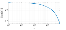
Figure 1: Convergence of the strategy profile $\boldsymbol{x}(k)$ to the consensus subspace. The matrix $\boldsymbol{L}$ is the Laplacian matrix associated to the multiplier graph.

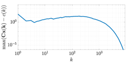
Figure 2: Asymptotic satisfaction of the time-varying affine coupling constraints $\boldsymbol{Cx}(k)\leq c(k)$.

The trajectory of the profile strategy generated by TV–Prox–GNWE converges to the consensus subspace, this is shown in Fig. 1, by means of the Laplacian matrix $\boldsymbol{L}$ of the multiplier graph. The initial strategy profile $\boldsymbol{x}(0)$ is randomly chosen in $\boldsymbol{\Omega}$. As expected from the result in Theorem 1, the constraints are satisfied asymptotically, see Fig. 2.

VI Conclusion and outlook

In multi-agent network games, subject to time-varying coupling constraints and time-varying communication network, described by strongly connected digraphs, agents can fail to converge when they adopt proximal dynamics. Nevertheless, it is developed an iterative equilibrium seeking algorithms (TV–Prox–GNWE) that ensures the global convergence of the agents’ strategies to an normalized equilibrium of the game, when it exists.

One of the most important open question in these type of problems regards the existence of an equilibrium point. This work can be improved with a new assumption for the equilibrium existence, which is general and easy to check.

-A Algorithm derivation

In this section, we propose the complete derivation of the iterative algorithm that we called TV–Prox–GNWE. We divide the derivation in two mains steps

1. Equilibria reformulation

2. Modified proximal point algorithm

-A1 Equilibria reformulation

the set of pn-ENWE, defined by the two equalities in (8), can be equivalently rephrased as the set of fixed points of a suitable mappings. First, we introduce the block-diagonal proximal operator

$$\boldsymbol{\textrm{prox}_{f}}\left(\begin{bmatrix}z_{1}\\ \vdots\\ z_{N}\end{bmatrix}\right):=\begin{bmatrix}\textrm{prox}_{\bar{f}_{1}}(z_{1})\\ \vdots\\ \textrm{prox}_{\bar{f}_{N}}(z_{N})\end{bmatrix}.$$ (11)

In (8), the first equality is equivalent to

$$\overline{\boldsymbol{x}}=\cap_{k>\bar{k}}\>\boldsymbol{\textrm{prox}_{f}}(\boldsymbol{A}(k)\boldsymbol{x}-\boldsymbol{\Lambda}(k)\boldsymbol{C}^{\top}(k)\overline{\sigma})\>,$$

where $\boldsymbol{A}(k)\coloneqq A(k)\otimes I_{n}$ and $\boldsymbol{\Lambda}(k)={\mathrm{diag}}((\alpha_{i}(k))_{i\in\mathcal{N}})\otimes I_{n}$. The second equality holds true if and only if $\overline{\sigma}=\textrm{proj}_{{\mathbb{R}}^{M}}(\overline{\sigma}+\boldsymbol{C}(k)\boldsymbol{\overline{x}}-c(k))$.

In order to describe via operators these two relations, we define the static mappings

$$\boldsymbol{\mathcal{R}}:=\mathrm{diag}(\boldsymbol{\textrm{prox}_{f}},\>\textrm{proj}_{{\mathbb{R}}^{M}_{\geq 0}})$$ (12)

and the time-varying affine one $\boldsymbol{\mathcal{G}}_{k}:{\mathbb{R}}^{nN+M}\rightarrow{\mathbb{R}}^{nN+M}$ as

$$\begin{split}\boldsymbol{\mathcal{G}}_{k}(\cdot)&:=\boldsymbol{G}\,\cdot+\begin{bmatrix}\boldsymbol{0}\\ c(k)\end{bmatrix}\\ &:=\begin{bmatrix}\boldsymbol{A}(k)&-\boldsymbol{\Lambda}(k)\boldsymbol{C}^{\top}(k)\\ C(k)&I\end{bmatrix}\cdot-\begin{bmatrix}\boldsymbol{0}\\ c(k)\end{bmatrix}\>.\end{split}$$ (13)

As a result, the dynamics of the game result equal to

$$\begin{bmatrix}\boldsymbol{x}(k+1)\\ \sigma(k+1)\end{bmatrix}=\boldsymbol{\mathcal{R}}\circ\boldsymbol{\mathcal{G}}_{k}\left(\begin{bmatrix}\boldsymbol{x}(k)\\ \sigma(k)\end{bmatrix}\right)\>.$$ (14)

We exploit this new compact form to describe the set of pn–ENWE via the fixed points of $\boldsymbol{\mathcal{R}}\circ\boldsymbol{\mathcal{G}}_{k}$. In particular, by Definiton 3, a pair $(\bar{\boldsymbol{x}},\bar{\sigma})$ is a pn–ENWE of the game in (4) if and only if $\mathrm{col}((\bar{\boldsymbol{x}},\bar{\sigma}))\in\cap_{k>\bar{k}}{\mathrm{fix}}(\boldsymbol{\mathcal{R}}\circ\boldsymbol{\mathcal{G}}_{k})$. Furthermore, from Lemma 1, we also know that a pn–ENWE is a p–GNWE of the original game. So, we focus on the design of an algorithm converging to the subset $\mathcal{E}$ for which we can take advantage of this new formulation.

A useful tool to solve fixed point seeking problem is to reformulate it as a zero finding problem, as done in the next lemma, see [28, Ch. 26].

Lemma 2 ([28, Prop. 26.1 (iv)])

Let $\boldsymbol{\mathcal{B}}:=F\times N_{{\mathbb{R}}^{M}_{\geq 0}}$, with $F:=\prod_{i=1}^{N}\partial\bar{f}_{i}$. Then,

$${\mathrm{fix}}\left(\boldsymbol{\mathcal{R}}\circ\boldsymbol{\mathcal{G}}_{k}\right)=\textrm{zer}\left(\boldsymbol{\mathcal{A}}_{k}\right)\>,$$

where $\boldsymbol{\mathcal{A}}_{k}\coloneqq\boldsymbol{\mathcal{B}}+\textrm{Id}-\boldsymbol{\mathcal{G}}_{k}$.  ∎

-A2 Modified proximal point algorithm

we describe in details the passages to develop the iterative algorithm solving the zero finding problem associated to the operator $\boldsymbol{\mathcal{A}}_{k}$, and, as a consequence, the original one of finding pn–ENWE of (4). We adopt a modified version of the proximal point algorithm (PPP) (see [28, Prop. 23.39] for its standard formulation). In particular, the update rule is a preconditioned version of the PPP algorithm proposed in [29, Eq. 4.18], after defining $\boldsymbol{\varpi}:=\mathrm{col}(\boldsymbol{x}(k),\,\sigma(k))$ and $\boldsymbol{\varpi}^{+}:=\mathrm{col}(\boldsymbol{x}(k+1),\,\sigma(k+1))$, it can be rewritten as

$$\tilde{\boldsymbol{\varpi}} =\mathrm{J}_{\Phi^{-1}(k)\boldsymbol{\mathcal{A}}_{k}}\boldsymbol{\varpi}$$ (15a)

$$\boldsymbol{\varpi}^{+} =\boldsymbol{\varpi}+\gamma(k)\boldsymbol{\bar{Q}}(k)\Phi(k)(\tilde{\boldsymbol{\varpi}}-\boldsymbol{\varpi})$$ (15b)

where and $\gamma(k)>0$ is the step–size of the algorithm and $\boldsymbol{\bar{Q}}(k)\coloneqq{\mathrm{diag}}(\boldsymbol{Q}(k),I)$. The preconditioning matrix is chosen as

$$\Phi(k):=\begin{bmatrix}\boldsymbol{\delta}^{-1}(k)+\boldsymbol{A}(k)&-\boldsymbol{\Lambda}(k)C(k)^{\top}\\ C(k)&\beta(k)I_{M}\end{bmatrix}$$ (16)

where $\beta(k)\in{\mathbb{R}}_{>0}$ and $\boldsymbol{\delta}(k)\coloneqq{\mathrm{diag}}((\delta_{i}(k))_{i\in\mathcal{N}})\otimes I_{n}$. The self-adjoint and skew symmetric components are defined as $U(k):=(\Phi(k)+\Phi^{\top}(k))/2$ and $S(k):=(\Phi(k)-\Phi^{\top}(k))/2$. Due to the non symmetric preconditioning the resolvent operator takes the form

$$\mathrm{J}_{\Phi^{-1}(k)\boldsymbol{\mathcal{A}}_{k}}:=\mathrm{J}_{U^{-1}(k)(\boldsymbol{\mathcal{A}}_{k}+S(k))}(\textrm{Id}+U^{-1}(k)S(k))\>.$$

The parameters $\boldsymbol{\delta}(k)$ and $\beta(k)$ in the preconditioning have to be chosen such that $U(k)\succ 0$ and $\lVert\boldsymbol{\bar{Q}}(k)U(k)\rVert\leq\gamma^{-1}(k)$. This can be done via the Gerschgorin Circle Theorem for partitioned matrices (more stringent but more involved bounds can be obtained via [30, Th. 2.1]). The resulting bounds are reported in (10).

Using a reasoning akin to the one in [29, Proof of Th. 4.2], one can show that, at every time instant $k$, the set of fixed points of the mapping describing the update in (15a)–(15b) coincides with ${\mathrm{zer}}(\boldsymbol{\mathcal{A}}_{k})$.

Finally, we are ready for the complete derivation of the algorithm by explicitly compute the local update rules of the agents and of the central coordinator. We omit the time dependency in the following formulas.

First, we focus on (15a) , so

$$\tilde{\boldsymbol{\varpi}}=\mathrm{J}_{U^{-1}(\boldsymbol{\mathcal{A}}+S)}(\textrm{Id}+U^{-1}S)\boldsymbol{\varpi}$$ (17a)

$$\tilde{\boldsymbol{\varpi}}+U^{-1}(\boldsymbol{\mathcal{A}}+S)\tilde{\boldsymbol{\varpi}}\ni\boldsymbol{\varpi}+U^{-1}S\boldsymbol{\varpi}$$ (17b)

$$\boldsymbol{0}\in U(\tilde{\boldsymbol{\varpi}}-\boldsymbol{\varpi})+\boldsymbol{\mathcal{A}}\tilde{\boldsymbol{\varpi}}+S(\tilde{\boldsymbol{\varpi}}-\boldsymbol{\varpi})$$ (17c)

$$\boldsymbol{0}\in\Phi(\tilde{\boldsymbol{\varpi}}-\boldsymbol{\varpi})+\boldsymbol{\mathcal{A}}\tilde{\boldsymbol{\varpi}}$$ (17d)

By solving the first row block of (17d), i.e. $\boldsymbol{0}\in(\boldsymbol{\delta}^{-1}+\boldsymbol{A})(\tilde{\boldsymbol{x}}-\boldsymbol{x})-\boldsymbol{\Lambda}C^{\top}(\tilde{\sigma}-\sigma)+F(\tilde{\boldsymbol{x}})+\tilde{\boldsymbol{x}}-\boldsymbol{A}\tilde{\boldsymbol{x}}+\boldsymbol{\Lambda}C^{\top}\tilde{\sigma}$ , we obtain

$$\boldsymbol{0}_{nN} \in\boldsymbol{\delta}^{-1}(\tilde{\boldsymbol{x}}-\boldsymbol{x})-\boldsymbol{A}\boldsymbol{x}+\boldsymbol{\Lambda}C^{\top}\sigma+F(\tilde{\boldsymbol{x}})+\tilde{\boldsymbol{x}}$$

$$\boldsymbol{0}_{nN} \in(\boldsymbol{\delta}^{-1}+I)\tilde{\boldsymbol{x}}+F(\tilde{\boldsymbol{x}})-\boldsymbol{\delta}^{-1}\boldsymbol{x}-\boldsymbol{A}\boldsymbol{x}+\boldsymbol{\Lambda}C^{\top}\sigma\>.$$

Let us define, with a small abuse of notation, the matrix $\frac{1}{\delta^{-1}+1}\coloneqq{\mathrm{diag}}\left(\big{(}\frac{1}{\boldsymbol{\delta}_{i}^{-1}+1}\big{)}_{i\in\mathcal{N}}\right)\otimes I_{n}$, then we attain

$$\boldsymbol{0}_{nN} \in\tilde{\boldsymbol{x}}+\textstyle{\frac{1}{\boldsymbol{\delta}^{-1}+1}}F(\tilde{\boldsymbol{x}})+\textstyle{\frac{1}{\boldsymbol{\delta}^{-1}+1}}\big{[}\boldsymbol{\Lambda}C^{\top}\sigma-\boldsymbol{\delta}^{-1}\boldsymbol{x}-\boldsymbol{A}\boldsymbol{x}\big{]}$$

$$\tilde{\boldsymbol{x}} =\mathrm{J}_{\scriptstyle{\frac{1}{\boldsymbol{\delta}^{-1}+1}}F}\left(\textstyle{\frac{1}{\boldsymbol{\delta}^{-1}+1}}\big{[}\boldsymbol{\delta}^{-1}\boldsymbol{x}+\boldsymbol{A}\boldsymbol{x}-\boldsymbol{\Lambda}C^{\top}\sigma\big{]}\right)\>.$$ (18)

The second row block instead reads as $\boldsymbol{0}\in C(\tilde{\boldsymbol{x}}-\boldsymbol{x})+\beta(\tilde{\sigma}-\sigma)+N_{{\mathbb{R}}^{M}_{\geq 0}}(\tilde{\sigma})+\tilde{\sigma}-C\tilde{\boldsymbol{x}}+c$, and leads to

$$\boldsymbol{0}_{M} \in-C\boldsymbol{x}+\beta(\tilde{\sigma}-\sigma)+N_{{\mathbb{R}}^{M}_{\geq 0}}(\tilde{\sigma})+c$$ (19a)

$$\tilde{\sigma} =\mathrm{J}_{N_{{\mathbb{R}}^{M}_{\geq 0}}}\left(\sigma+\textstyle{\frac{1}{\beta}}(C\boldsymbol{x}-c)\right)$$ (19b)

Combining (18) and (19b) together with (15b), leads to the final formulation for the TV–Prox–GNWE, its dynamics are shown in (9a) – (9d).

-B Convergence proof of TV–Prox–GNWE

In order to simplify the proofs proposed in the following, let us introduce some useful definition that will be adopted thorough the whole section. We define the two scalars $L_{k}$ and $m_{k}$, the former is the Lipschitz constant of $S(k)$ and the latter is such that $m_{k}\lVert x\rVert^{2}<\langle U(k)x,x\rangle$, this also implies that $\lVert U^{-1}(k)\rVert\leq m_{k}^{-1}$. Next, we define the time-varying matrix $K(k)\coloneqq\overline{\boldsymbol{Q}}_{k}U(k)$ and the scalars $\rho\coloneqq m_{k}^{-1}L_{k}$, $q_{m}\coloneqq\min_{i}[\boldsymbol{\overline{Q}}_{k}]_{ii}$ and $M_{k}\geq\lVert U(k)\rVert$. Notice that, without loss of generality, we can always choose the normalized version of the left Perron Frobenius eigenvector $q(k)$ of the matrix $A(k)$, so $\max_{i}[\boldsymbol{\overline{Q}}_{k}]_{ii}\leq 1$.

In the following, we also omit the time dependency of the operators when this does not lead to ambiguities. The proofs follow similar steps to the ones in [29, Prop.2.1 and 4.2], where the case of a static communication network is considered.

Lemma 3

For all $k\in{\mathbb{N}}$, consider the time-varying operator

$$\mathcal{T}_{\Phi}:=\mathrm{J}_{\Phi^{-1}\boldsymbol{\mathcal{A}}}+U^{-1}S(\mathrm{J}_{\Phi^{-1}\boldsymbol{\mathcal{A}}}-\textrm{Id})\>,$$ (20)

then the following hold:

1. $\mathcal{T}_{\Phi}$is quasi-nonexpansive in the space $\mathcal{H}_{K}$,

2. if $L_{k}\leq m_{k}$, then ${\mathrm{fix}}(\mathcal{T}_{\Phi})={\mathrm{zer}}(\boldsymbol{\mathcal{A}})$ . ∎

Proof:

(i) From the proof of [19, Th. 5], the operator $\boldsymbol{\mathcal{A}}\coloneqq\boldsymbol{\mathcal{B}}+\textrm{Id}-\boldsymbol{\mathcal{G}}_{k}$ is maximally monotone in $\mathcal{H}_{\overline{\boldsymbol{Q}}}$ for all $k\in{\mathbb{N}}$. The operator $S$ is also maximally monotone, since it is a skew-symmetric matrix, [28, Ex. 20.30]. Next, we define the two auxiliary operators $\mathcal{M}=U^{-1}(\boldsymbol{\mathcal{A}}+S)$ and $\mathcal{D}=-U^{-1}S$. It is easy to see that $\mathcal{A}$ is monotone and $\mathcal{D}$ is monotone and $\rho$-Lipschitz, , in $\mathcal{H}_{K}$. From [29, Prop. 2.1 (3)], we obtain that for $\varpi^{*}\in{\mathrm{fix}}(\mathcal{T}_{\Phi})$ it holds for some $\bar{\gamma}>0$

$$\lVert\mathcal{T}_{\Phi}\varpi-\varpi^{*}\rVert^{2}_{K}\leq\lVert\varpi-\varpi^{*}\rVert_{K}-(1+\rho^{2})\lVert\varpi-x\rVert^{2}_{K}$$ (21)

where $x\coloneqq\mathrm{J}_{\mathcal{M}}(\varpi-\mathcal{D}\varpi)$. Hence, we conclude that $\mathcal{T}_{\Phi}$ is quasi-nonexpansive in $\mathcal{H}_{K}$.

(ii) If $L_{k}\leq m_{k}$, then the result follows directly from [29, Prop. 2.1 (1)], where we considered $A\coloneqq\mathcal{M}$, $B_{1}=0$ and $B_{2}\coloneqq\mathcal{D}$. ∎

Proof of Theorem 1

Consider $\mathcal{T}_{\Phi}$, as in (20), then the following relation always holds

$$\overline{\boldsymbol{Q}}U(\textrm{Id}-\mathcal{T}_{\Phi})(x)=\overline{\boldsymbol{Q}}\Phi(x-\mathrm{J}_{\Phi^{-1}\boldsymbol{\mathcal{A}}})\,.$$ (22)

From Lemma 3 we know that $\mathcal{T}_{\Phi}$ is quasi-nonexpansive in $\mathcal{H}_{K}$, hence $\mathcal{S}:=(\textrm{Id}+\mathcal{T}_{\Phi})/2$ belongs to the class $\mathfrak{I}$ in $\mathcal{H}_{K}$, [21, Prop. 2.2(v)]. From [29, Prop. 4.1] and (22), we define the operator

$$\begin{split}\mathcal{W}_{\Phi}&:=\textrm{Id}-\lVert K\rVert^{-1}K(\textrm{Id}-\mathcal{S})\\ &=\textrm{Id}-\frac{1}{2}\lVert K\rVert^{-1}K(\textrm{Id}-\mathcal{T}_{\Phi})\>,\\ \end{split}$$ (23)

belonging to $\mathfrak{I}$ in $\mathcal{H}$ and ${\mathrm{fix}}(\mathcal{W}_{\Phi})={\mathrm{fix}}(\mathcal{T}_{\Phi})={\mathrm{zer}}(\boldsymbol{\mathcal{A}})$, where the last equality comes from Lemma 3. The update rule in (15) can be rewritten as

$$\boldsymbol{\varpi}^{+}=\boldsymbol{\varpi}+2\gamma\lVert K\rVert(\mathcal{W}_{\Phi}\boldsymbol{\varpi}-\boldsymbol{\varpi})\>,$$ (24)

where $\gamma\lVert K\rVert<1$ for all $k$, due to the choice of $\delta_{i}$ and $\beta$. Thus, from [21, Th. 4.2(ii) and 4.3], we have that $(\lVert\boldsymbol{\varpi}-\mathcal{W}_{\Phi}\boldsymbol{\varpi}\rVert^{2})_{k\in{\mathbb{N}}}$ is summable and converges in $\mathcal{H}$ to an element $\overline{\boldsymbol{\varpi}}\in\mathcal{E}_{c}$, hence to a pn-ENWE, if and only if every sequential cluster point of sequence belong to $\mathcal{E}_{c}$.

Toward this aim, we define $x_{\varpi}\coloneqq\mathrm{J}_{\Phi^{-1}\boldsymbol{\mathcal{A}}}(\varpi)$ then we prove that $\varpi-x_{\varpi}\rightarrow 0$ and $x_{\varpi}\rightarrow\overline{x}_{\varpi}\in{\mathrm{zer}}(\boldsymbol{\mathcal{A}})$, concluding the proof.

First, notice that, due to the choice of the coefficients $\boldsymbol{\delta}$ and $\beta$ in $\Phi(k)$, it holds

$$\begin{split}\lVert\boldsymbol{\varpi}-\mathcal{T}_{\Phi}\boldsymbol{\varpi}\rVert^{2}_{K}&\leq\lVert K^{-1}\rVert\lVert\boldsymbol{\varpi}-\mathcal{T}_{\Phi}\boldsymbol{\varpi}\rVert^{2}\\ &\leq 4m_{k}^{-1}M_{k}^{2}\lVert\boldsymbol{\varpi}-\mathcal{W}_{\Phi}\boldsymbol{\varpi}\rVert^{2}\rightarrow 0\>.\end{split}$$ (25)

Let us define $x_{\varpi}\coloneqq\mathrm{J}_{\bar{\gamma}\mathcal{A}}(\varpi-\bar{\gamma}U^{-1}S\varpi)$, Moreover, from (21), it follows

$$\begin{split}(1-\rho^{2})\lVert\varpi&-x_{\varpi}\rVert_{K}\leq\lVert\varpi-\varpi^{*}\rVert_{K}-\lVert\mathcal{T}_{\Phi}\varpi-\varpi\rVert_{K}\\ &=-\lVert\mathcal{T}_{\Phi}\varpi-\varpi\rVert_{K}-2\langle\mathcal{T}_{\Phi}\varpi-\varpi,\varpi-\varpi^{*}\rangle_{K}\\ &\leq-\lVert\mathcal{T}_{\Phi}\varpi-\varpi\rVert_{K}-2M_{k}\lVert\mathcal{T}_{\Phi}\varpi-\varpi\lVert_{K}\rVert\varpi-\varpi^{*}\rVert\end{split}$$

The above inequality leads to

$$(1-\rho^{2})m_{k}q_{m}\lVert\varpi-x_{\varpi}\rVert \leq-\lVert\mathcal{T}_{\Phi}\varpi-\varpi\rVert_{K}$$ (26)

$$-2M_{k}\lVert\mathcal{T}_{\Phi}\varpi-\varpi\lVert_{K}\rVert\varpi-\varpi^{*}\rVert$$

The sequence $(\lVert\varpi(k)-\varpi^{*}\rVert)_{k\in{\mathbb{N}}}$ is bounded and from (25) and (26), we deduce that $\varpi-x_{\varpi}\rightarrow 0$. Notice also that

$$\lVert\overline{Q}\Phi(\varpi-x_{\varpi})\rVert\leq(M_{k}+L)\lVert\varpi-x_{\varpi}\rVert\rightarrow 0\>.$$

From the definition of $x_{\varpi}$, it follows

$$u_{k}\coloneqq\overline{Q}\Phi(\varpi-x_{\varpi})\in\boldsymbol{\mathcal{A}}x_{\omega}\>.$$

Thus, since $u_{k}\rightarrow 0$, we conclude that $x_{\varpi}\rightarrow\overline{x}_{\varpi}\in{\mathrm{zer}}(\boldsymbol{\mathcal{A}})$.

∎

References

• [1] S. Grammatico, “Opinion dynamics are proximal dynamics in multi-agent network games,” in 2017 IEEE 56th Annual Conference on Decision and Control (CDC), Dec 2017, pp. 3835–3840.
• [2] J. Ghaderi and R. Srikant, “Opinion dynamics in social networks with stubborn agents: Equilibrium and convergence rate,” Automatica, vol. 50, pp. 3209–3215, 2014.
• [3] S. R. Etesami and T. Başar, “Game-theoretic analysis of the hegselmann-krause model for opinion dynamics in finite dimensions,” IEEE Trans. on Automatic Control, vol. 60, no. 7, pp. 1886–1897, 2015.
• [4] R. Jaina and J. Walrand, “An efficient Nash-implementation mechanism for network resource allocation,” Automatica, vol. 46, pp. 1276–1283, 2010.
• [5] C. Cenedese, G. Belgioioso, S. Grammatico, and M. Cao, “An asynchronous, forward-backward, distributed generalized nash equilibrium seeking algorithm,” in 2019 18th European Control Conference (ECC), June 2019, pp. 3508–3513.
• [6] D. Callaway, “Tapping the energy storage potential in electric loads to deliver load following and regulation, with application to wind energy,” Energy Conversion and Management, vol. 50, no. 5, pp. 1389–1400, 2009.
• [7] F. Dörfler, J. Simpson-Porco, and F. Bullo, “Breaking the hierarchy: Distributed control and economic optimality in microgrids,” IEEE Trans. on Control of Network Systems, vol. 3, no. 3, pp. 241–253, 2016.
• [8] S. Grammatico, “Proximal dynamics in multi-agent network games,” IEEE Trans. on Control of Network Systems, vol. 5, no. 4, pp. 1707–1716, Dec 2018.
• [9] S. Martínez, F. Bullo, J. Cortés, and E. Frazzoli, “On synchronous robotic networks – Part i: Models, tasks, and complexity,” IEEE Trans. on Automatic Control, vol. 52, pp. 2199–2213, 2007.
• [10] A. Simonetto and G. Leus, “Distributed maximum likelihood sensor network localization,” IEEE Transactions on Signal Processing, vol. 62, no. 6, pp. 1424–1437, March 2014.
• [11] A. Nedić and A. Olshevsky, “Distributed optimization over time-varying directed graphs,” IEEE Transactions on Automatic Control, vol. 60, no. 3, pp. 601–615, March 2015.
• [12] A. Nedić, A. Olshevsky, and W. Shi, “Achieving geometric convergence for distributed optimization over time-varying graphs,” SIAM Journal on Optimization, vol. 27, no. 4, pp. 2597–2633, 2017.
• [13] N. Li and J. R. Marden, “Designing games for distributed optimization with a time varying communication graph,” pp. 7764–7769, Dec 2012.
• [14] F. Facchinei and C. Kanzow, “Generalized Nash equilibrium problems,” A Quarterly Journal of Operations Research, Springer, vol. 5, pp. 173–210, 2007.
• [15] P. Yi and L. Pavel, “A distributed primal-dual algorithm for computation of generalized Nash equilibria via operator splitting methods,” in 2017 IEEE 56th Annual Conference on Decision and Control (CDC), Dec 2017, pp. 3841–3846.
• [16] G. Belgioioso and S. Grammatico, “Projected-gradient algorithms for generalized equilibrium seeking in aggregative games arepreconditioned forward-backward methods,” pp. 2188–2193, June 2018.
• [17] J. Koshal, A. Nedić, and U. Shanbhag, “Distributed algorithms for aggregative games on graphs,” Operations Research, vol. 64, no. 3, pp. 680–704, 2016.
• [18] C. Cenedese, Y. Kawano, S. Grammatico, and M. Cao, “Towards time-varying proximal dynamics in multi-agent network games,” in 2018 IEEE Conference on Decision and Control (CDC), Dec 2018, pp. 4378–4383.
• [19] C. Cenedese, G. Belgioioso, Y. Kawano, S. Grammatico, and M. Cao, “Asynchronous and time-varying proximal type dynamics multi-agent network games,” arXiv e-prints, p. arXiv:1909.11203, Sep 2019.
• [20] D. Fullmer and A. S. Morse, “A distributed algorithm for computing a common fixed point of a finite family of paracontractions,” IEEE Transactions on Automatic Control, vol. 63, no. 9, pp. 2833–2843, Sep. 2018.
• [21] P. Combettes, “Quasi-Fejérian analysis of some optimization algorithms,” in Studies in Computational Mathematics, Inherently parallel algorithms in feasibility and optimization and their applications.   Elsevier, 2001, pp. 115–152.
• [22] H. H. Bauschke and P. L. Combettes, Convex analysis and monotone operator theory in Hilbert spaces.   Springer, 2010.
• [23] R. Cominetti, F. Facchinei, and J. Lasserre, Modern optimization modelling techniques.   Birkhäuser, 2010.
• [24] G. Belgioioso and S. Grammatico, “Semi-decentralized Nash equilibrium seeking in aggregative games with separable coupling constraints and non-differentiable cost functions,” IEEE Control Systems Letters, vol. 1, no. 2, pp. 400–405, Oct 2017.
• [25] J. Rosen, “Existence and uniqueness of equilibrium points for concave n-person games,” Econometrica, vol. 33, pp. 520–534, 1965.
• [26] P. L. Combettes and I. Yamada, “Compositions and convex combinations of averaged nonexpansive operators,” Journal of Mathematical Analysis and Applications, pp. 55–70, 2015.
• [27] A. Nedić, A. Ozdaglar, and P. Parrillo, “Constrained consensus and optimization in multi-agent networks,” IEEE Trans. on Automatic Control, vol. 55, no. 4, pp. 922–938, 2010.
• [28] H. H. Bauschke and P. L. Combettes, Convex Analysis and Monotone Operator Theory in Hilbert Spaces, 2010.
• [29] L. Briceno-Arias and D. Davis, “Forward-backward-half forward algorithm for solving monotone inclusions,” SIAM Journal on Optimization, vol. 28, no. 4, pp. 2839–2871, 2018.
• [30] A. Melman, “Generalizations of gershgorin disks and polynomial zeros,” Proceedings of the American Mathematical Society, vol. 138, no. 7, pp. 2349–2364, 2010.