Defective Convolutional Networks

Abstract

Robustness of convolutional neural networks (CNNs) has gained in importance on account of adversarial examples, i.e., inputs added as well-designed perturbations that are imperceptible to humans but can cause the model to predict incorrectly. Recent research suggests that the noises in adversarial examples break the textural structure, which eventually leads to wrong predictions. To mitigate the threat of such adversarial attacks, we propose defective convolutional networks that make predictions relying less on textural information but more on shape information by properly integrating defective convolutional layers into standard CNNs. The defective convolutional layers contain defective neurons whose activations are set to be a constant function. As defective neurons contain no information and are far different from standard neurons in its spatial neighborhood, the textural features cannot be accurately extracted, and so the model has to seek other features for classification, such as the shape. We show extensive evidence to justify our proposal and demonstrate that defective CNNs can defense against black-box attacks better than standard CNNs. In particular, they achieve state-of-the-art performance against transfer-based attacks without any adversarial training being applied.

1 Introduction

Deep learning [24], especially deep Convolutional Neural Network (CNN) [25], has led to state-of-the-art results spanning many machine learning fields [15, 34]. Despite the great success in numerous applications, recent studies show that deep CNNs are vulnerable to some well-designed input samples named as Adversarial Examples [41, 3]. Take the task of image classification as an example, for almost every commonly used well-performed CNN, attackers are able to construct a small perturbation on an input image, which is almost imperceptible to humans but can make the model give a wrong prediction. The problem is serious as some well-designed adversarial examples can be transferred among different kinds of CNN architectures [32]. As a result, a machine learning system can be easily attacked even if the attacker does not have access to the model parameters.

There is a rapidly growing body of work on how to obtain a robust CNN, mainly based on adversarial training [41, 29, 14, 21]. However, those methods need lots of extra computation to obtain adversarial examples at each time step and tend to overfit the attacking method used in training [5]. In this paper, we tackle the problem in a perspective different from most existing methods. In particular, we explore the possibility of designing new CNN architectures which can be trained using standard optimization methods on standard benchmark datasets and can enjoy robustness by themselves, without appealing to other techniques. Recent studies [11, 12, 2] show that the predictions of standard CNNs mainly depend on the texture of objects. The textural information has a high degree of redundancy and may be easily injected with adversarial noise  [45, 17]. Also, [27] finds adversarial attack methods may perturb local patches to contain textural features of incorrect classes. All the literature suggests that the wrong prediction by CNNs for adversarial examples mainly comes from the change in the textural information. The small perturbation of adversarial examples will change the textures and eventually affect the features extracted by the CNNs. Therefore, a natural way to avoid adversarial examples is to let the CNN make predictions relying less on textures but more on other information, such as the shape, which cannot be severely affected by small perturbations.

In real practice, sometimes a camera might have mechanical failures which cause the output image to have many defective pixels (such pixels are always black in all images). Nonetheless, humans can still recognize objects in the image with defective pixels since we are able to classify the objects even in the absence of local textural information. Motivated by this, we introduce the concept of defectiveness into the convolutional neural networks: we call a neuron a defective neuron if its output value is fixed to zero no matter what input signal is received; similary, a convolutional layer is a defective convolutional layer if it contains defective neurons. Before training, we replace the standard convolutional layers with the defective version on a standard CNN and train the network in the standard way. As defective neurons of the defective convolutional layer contain no information and are very different from their spatial neighbors, the textural information cannot be accurately extracted from the bottom defective layers to top layers. Therefore, we destroy local textural information to a certain extent and prompt the neural network to rely more on other information for classification. We call the architecture deployed with defective convolutional layers as defective convolutional network.

We find that applying the defective convolutional layers to the bottom layers of the network and introducing various patterns for defective neurons arrangement across channels are crucial for robustness. In summary, our main contributions are:

• We propose the Defective CNNs that, compared to the standard CNNs, relies less on textures and more on shapes of the inputs for making predictions. The adversarial robustness is implanted in the design of Defective CNNs, because most adversarial attacks produce perturbations that leave the underlying shape intact, only to manipulate the local texture of the inputs.

• Experimental results show that Defective CNN has superior defense performance than standard CNN against transfer-based attacks, decision-based attacks, additive Gaussian noise, and grey-box attacks.

• Using the standard training method, Defective CNN achieves state-of-the-art results against two transfer-based black-box attacks while maintaining high accuracy on clean test data.

2 Related Work

Various methods have been proposed to defend against adversarial examples. One line of research is to derive a meaningful optimization objective and optimize the model by adversarial training [41, 29, 14, 21]. The high-level idea of these works is that if we can predict the potential attack to the model during optimization, then we can give the attacked sample a correct signal and use it during training. Another line of research is to take an adjustment to the input image before letting it go through the deep neural network [26, 37, 35, 39, 44]. The basic intuition behind this is that if we can clean the adversarial attack to a certain extent, then such attacks can be defended. Although these methods achieve some success, a major difficulty is that it needs a large extra cost to collect adversarial examples and hard to apply on large-scale datasets.

Several studies [11, 12, 2] show that the prediction of CNNs is mainly from the texture of objects but not the shape. Also, [27] found that adversarial examples usually perturb a patch of the original image so that the perturbed patch looks like the texture of incorrect classes. For example, the adversarial example of the panda image is misclassified as a monkey because a patch of the panda skin is perturbed adversarially so that it alone looks like the face of a monkey (see Figure 11 in [27]). All previous works above suggest that the CNN learns textural information more than shape and the adversarial attack might come from textural-level perturbations. This is also correlated with robust features [43, 22, 17, 45] which has attracted more interest recently. Pixels which encode textural information contain high redundancy and may be easily deteriorated to the distribution of incorrect classes. However, shape information is more compact and might be a more robust feature.

3 Defective Convolutional Neural Network

3.1 Design of Defective Convolutional Layers

In this subsection, we introduce our proposed defective convolutional neural networks and discuss the differences between our proposed method and related topics.

First, we briefly introduce the notations. For one convolutional layer, denote $x$ as the input and $z$ as the output of neurons in the layer. Note that $x$ may be the input image or the output of the last convolutional layer. The input $x$ is usually a $M\times N\times K$ tensor in which $M/N$ are the height/width of a feature map, and $K$ is the number of feature maps, or equivalently, channels. Denote $w$ and $b$ as the parameters (e.g., the weights and biases) of the convolutional kernel. Then a standard convolutional layer can be mathematically defined as below.

Standard convolutional layer:

$$x^{\prime} = w\otimes_{\text{conv}}x+b,$$ (1)

$$z = f(x^{\prime}),$$ (2)

where $f(\cdot)$ is a non-linear activation function such as ReLU and $\otimes_{\text{conv}}$ is the convolutional operation.

The convolutional filter receives signals in a patch and extracts local textural information from the patch. As mentioned in the introduction, recent works suggest that the prediction of standard CNNs strongly depends on such textural information, and noises imposed on the texture may lead to wrong predictions. Therefore, we hope to learn a feature extractor which does not solely rely on textural features and also considers other information. To achieve this goal, we introduce the defective convolutional layer in which some neurons are purposely designed to be corrupted. Define $M_{\text{defect}}$ to be a binary matrix of size $M\times N\times K$. Our defective convolutional layer is defined as follows.

Defective convolutional layer:

$$x^{\prime} = w\otimes_{\text{conv}}x+b,$$ (3)

$$z^{\prime} = f(x^{\prime})$$ (4)

$$z = M_{\text{defect}}*z^{\prime},$$ (5)

where $*$ denotes element-wise product. $M_{\text{defect}}$ is a fixed matrix and is not learnable during training and testing. A simple visualization of a defective convolutional layer is shown in Figure 1. From the figure, we can see that $M_{\text{defect}}$ plays a role of “masking” out values of some neurons in the layer. This disturbs the distribution of local textural information and decouples the correlation among neurons. With the masked output $z$ as input, the feature extractor of the next convolutional layer cannot accurately capture the local textural feature from $x$. As a consequence, the textural information is hard to pass through the defective CNN from bottom to top. To produce accurate predictions, the deep neural network has to find relevant signals other than the texture, e.g., the shape. Those corrupted neurons have no severe impact on the extraction of shape information since neighbors of those neurons in the same filter are still capable of passing the shape information to the next layer.

In this paper, we find that simply setting $M_{\text{defect}}$ by random initialization is already helpful for learning a robust CNN. Before training, we sample each entry in $M_{\text{defect}}$ using Bernoulli distribution with keep probability $p$ and then fix $M_{\text{defect}}$ during training and testing. More discussions and ablation studies are provided in Section 4.

Figure 1: An illustration of three channels (neuron-wise) from standard convolutional layer to defective convolutional layer. Black neurons are the defective neurons which are randomly selected. The output of defective neurons is fixed to zero during both training and testing phases. Note that the number of parameters in the network is not reduced after including defective neurons.

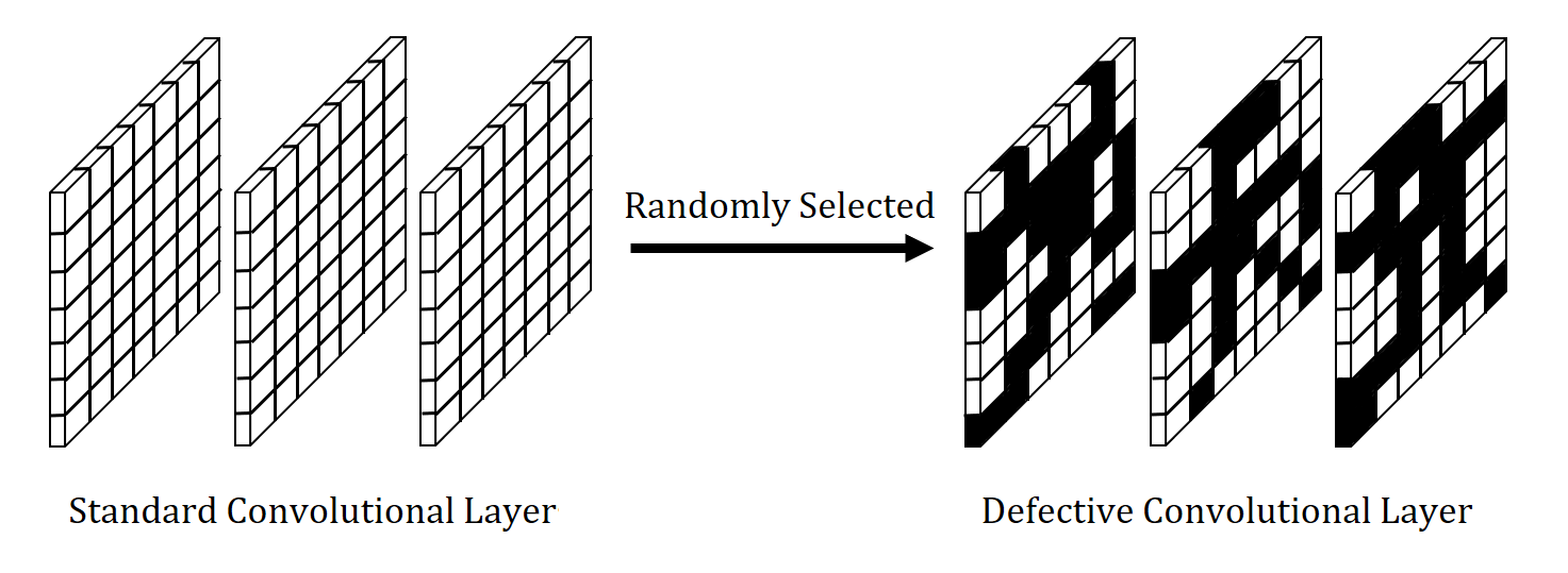
As can be seen from Equation (3)-(5), the implementation of our defective convolutional layer is similar to the dropout operation [38]. To demonstrate the relationship and differences, we mathematically define the dropout as below.

Standard convolutional layer + dropout:

$$M_{\text{dp}} \sim \text{Bernoulli}(p)$$ (6)

$$x^{\prime} = w\otimes_{\text{conv}}x+b$$ (7)

$$z^{\prime} = f(x^{\prime})$$ (8)

$$z = M_{\text{dp}}*z^{\prime}.$$ (9)

The shape of $M_{\text{dp}}$ is the same as $M_{\text{defect}}$, and the value of each entry in $M_{\text{dp}}$ is sampled in each batch using some sampling strategies at each step during training. Generally, entries in $M_{\text{dp}}$ are independent and identically sampled in an online fashion using Bernoulli distribution with keep probability $p$. DropBlock [13] dropouts a connected block in each channel. In SpatialDropout [42], the dropout masks apply to whole channels. Note that the masked unit of our proposed method is a single neuron.

There are several significant differences between dropout and defective convolutional layer. First, the motivations behind the two methods are quite different. Dropout tries to reduce overfitting by preventing co-adaptations on training data. As the neurons in the feature maps still have full access to local textural features in testing, the model does not have to learn shape features. However, in our proposed architecture, defective neurons are fixed to be corrupted, and such neurons cannot contribute to local features. Second, the binary matrix $M_{\text{dp}}$ is sampled online during training and is removed during testing, while the binary matrix $M_{\text{defect}}$ in defective convolutional layers is predefined and keeps fixed in both training and testing. Third, places to apply and values of the keep probability $p$ for two methods are different. Dropout methods are usually applied to top layers, and $p$ is set to be large (e.g., $0.9$)  [42, 13]. For defective convolutional layer, we find using a small $p$ (e.g., $0.1$) and applying it to bottom layers are more effective.

3.2 Defective CNN Relies Less on Texture but More on Shape

In the defective CNN, some neurons are set to be corrupted during both training and testing, and we argue that this design can help the CNN make prediction relying less on textural information but more on shape information. In this subsection, we provide some empirical analyses to verify our intuition.

We design a particular image manipulation in which the local texture of the object in an image is preserved while the shape is destroyed. In detail, we divide an image into $k\times k$ patches and randomly relocate those patches to form a new image. A typical example is shown in Figure 2. By relocating the patches, it is even hard for a human to recognize the object in the picture when $k$ is large.

(a) original image

(b) $2\times 2$ patches

(c) $4\times 4$ patches

(d) $8\times 8$ patches

Figure 2: An example image that is randomly shuffled after being divided into $2\times 2$, $4\times 4$ and $8\times 8$ patches respectively.

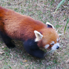
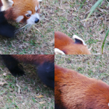
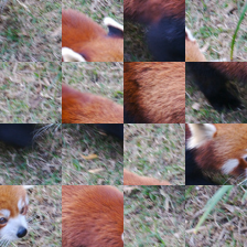
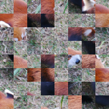
We manipulate a set of images and test whether a defective CNN and a standard CNN can make correct predictions. The experimental details are described as follows. First, we construct a defective CNN by applying defective convolutional layers to the bottom layers of a standard ResNet-18, and train the defective CNN along with a standard ResNet-18 on the ImageNet dataset. Then, we sample images from the validation set which are predicted correctly by both two CNNs. We make manipulations to the sampled images by setting $k\in\{2,4,8\}$, feed these images to the networks and check their classification accuracy. The results in Table 1 show that when the shape information is destroyed but the local textural information is preserved, the defective CNN performs consistently worse than standard CNN, verifying that defective CNN makes predictions relying less on local textural information but more on shape information.

Model	$2\times 2$	$4\times 4$	$8\times 8$	IN $\rightarrow$ SIN
Standard CNN	99.53%	84.36%	20.08%	15.33%
Defective CNN	96.32%	56.91%	9.04%	20.20%

Table 1: Left three columns are the accuracy of classifying randomly shuffled images. The rightmost column is the accuracy of training on ImageNet and testing on Stylized-ImageNet. More results for different architectures can be found in Appendix 0.A.5.

We also test the models on the Stylized-ImageNet [12], a stylized version of ImageNet, where the local textures of images are heavily distorted, while global object shapes remain. A model that more focuses on the shape cues should achieve higher performance on the Stylized-ImageNet while it is trained on the ImageNet. We test on the same model used in the randomly shuffled experiments by feeding the images from the validation set of Stylized-ImageNet whose corresponding images in ImageNet can be correctly classified by both two tested models. The result is listed in Table 1. It shows that the Defective CNN achieves higher transferring accuracy than the Standard CNN and thus verify our intuition.

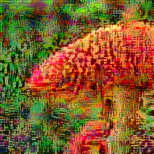
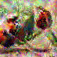
From another perspective, if a model makes predictions relying less on textural information but more on shape information, the manipulation of the shape of objects will play a larger role in designing adversarial examples. To verify this, we train a defective CNN on CIFAR-10 dataset and Tiny-ImageNet dataset, and then apply an iterative attack method MIFGSM [9] on the validation set. Some examples are shown in Figure 3 and Appendix 0.B. We can see that adversarial examples against the defective CNN change the shape of the objects and may even fool humans as well. The phenomena not only supports the intuition, but also is consistent with the findings in [43] that the representations learned by robust models tend to align better with salient data characteristics.

(a) Dog

(b) Bird

(c) Frog

(d) Ship

(e) Mushroom

(f) Ladybug

(g) Airplane

(h) Ship

(i) Truck

(j) Automobile

(k) Goldfish

(l) Fly

Figure 3: Adversarial examples generated by Defective CNNs with perturbation scale $\ell_{\infty}\in\{16,32\}$. First row: the adversarial examples and the labels predicted by the CNNs. Second row: the corresponding original images and the ground truth labels. Detailed experimental settings and more examples can be found in Appendix 0.B.

Furthermore, perturbations generated by standard CNNs and additive Gaussian noises usually change the textural information but hard to affect the shape information. A model is supposed to defend these attacks on textures better if it relies much on shape information for predictions. In Section 4, we show that defective CNNs achieve higher defense performance than standard CNN against the two types of attack, further supporting our intuitions.

4 Experiments

In this section, we provide extensive experimental analyses on the robustness of defective CNNs against black-box attacks. To better evaluate this point, we suggest that we should examine the target model against transfer-based attacks, decision-based attacks, and additive Gaussian noise.

In real-world tasks, attackers usually cannot access the parameters of the target models and thus need to transfer adversarial examples generated by their models. This setting of attack is referred to as transfer-based attacks [28, 23]. Sometimes, attackers can get the final model decision and raise the more powerful decision-based attacks [4]. Both the two types of black-box attack are available in most real-world scenarios and should be considered. Recently, [10] bridge the adversarial robustness and corruption robustness [16], and points out that a successful adversarial defend method should also effectively defense against additive Gaussian noise. Also, the additive Gaussian noise can be viewed as a type of black-box attack since the noise distribution has nothing to do with the parameters of tested models. Therefore, we also test the performance of target models against additive Gaussian noise.

We first test the robustness of defective CNN against transfer-based attacks, decision-based attacks, additive Gaussian noise, and then make ablation studies on possible design choices of defective CNN. Since we alter the network architecture and may pick up different potentially robust features following the argument in [22], we also carefully study the robustness in the gray-box setting. Due to space limitation, we list the results of gray-box attacks, white-box attacks, and transfer-based attacks from ensemble models in Appendix 0.A.

Note that, in this paper, all the successful defense rates except the rates listed in Table 2 are calculated on the samples whose corresponding original images can be classified correctly by the tested model. This can erase the influence of test accuracy that different models have different test accuracy on clean data, and thus help evaluate the robustness of models.

4.1 Transfer-based Attack

4.1.1 Experimental Settings

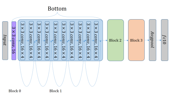
In this subsection, we evaluate the defense performance of networks with defective convolutional layers against transfer-based attacks. We compare our proposed method with state-of-the-art defense methods [5, 29]. For fair comparisons, we follow [5] to generate adversarial examples using wide residual networks [46] with a depth of $32$ and a width factor of $4$. The $4$-block structure of ResNet-32 is shown in Appendix 0.C. The blocks are labeled $0,1,2,3$ and the $0^{\text{th}}$ block is the first convolution layer. Both FGSM [14] and PGD [23] attacks are run on the entire validation set of CIFAR-10 dataset. These two methods both have $\ell_{\infty}$ perturbation scale $8$ and PGD runs for $7$ gradient descent steps with step size $2$. The generated adversarial examples are used to attack target networks. For the target network, we use the same structure but applying defective convolutional layers to the $0^{\text{th}}$ and $1^{\text{st}}$ blocks with keep probability $p=0.07$ and train the model using standard optimization method. As is mentioned in Section 3, our proposed method is essentially different from dropout, and thus we also take dropout methods as baselines. More specifically, we test SpatialDropout and DropBlock. For both methods, we follow the instruction from [13] to apply dropout to the $3^{\text{rd}}$ block with $p=0.9$. The block of DropBlock is set to be a $3\times 3$ square. Training details and curves can be found in Appendix 0.D.

Second, we test our proposed method in different architectures on the CIFAR-10 dataset. We apply defective convolutional layers, in a way which is similar to the experiment above, to five popular network architectures: ResNet-18 [15], ResNet-50, DenseNet-121 [20], SENet-18 [18] and VGG-19 [36]. For each architecture, we replace the standard convolutional layer with the defective version on the bottom layers. We then test the black-box defense performance against transfer-based attacks on 5000 samples from the validation set. Adversarial examples are generated by PGD, which runs for $20$ steps with step size $1$ and the $\ell_{\infty}$ perturbation scale is set to $16$. More results on the MNIST dataset and illustrations of where to apply the defective layers can be found in Appendix 0.A and 0.C.

4.1.2 Experimental Results

First, we compare with two strong defense methods [29, 5] and two dropout methods [42, 13]. The results are listed in Table 2. [29] is one adversarial training method that directly optimizes on adversarial examples in an online way. Based on adversarial training, [5] proposed a method that discretizes inputs and achieved higher accuracy against transfer-based attack. The results show the strengths of our proposed method on both robustness and generalization, even though our model is only trained on clean data. In addition, from the results of two dropout methods, we can conclude that spatial dropout and drop block do not improve the robustness of standard CNNs.

Model	FGSM	PGD	Test Accuracy
Standard CNN	52.88%	15.98%	95.39%
Standard CNN + SD [42]	51.63%	14.28%	95.98%
Standard CNN + DB [13]	51.55%	12.71%	95.81%
Adversarial Training [29]	85.60%	86.00%	87.30%
Thermometer(16) [5]	-	88.25%	89.88%
Thermometer(32) [5]	-	86.60%	90.30%
Defective CNN	86.24%	88.43%	91.12%

Table 2: Black-box defense performances against transfer-based attacks. SD and DB denote spatial dropout and drop block, respectively. Detailed settings are listed in Section 4.1.1.

Second, we list the black-box defense results of applying defective convolutional layers to various architectures in Table 3. The results show that defective convolutional layers consistently improve the robustness of various network architectures against transfer-based attacks.

Architecture	ResNet-18	ResNet-50	DenseNet-121	SENet-18	VGG-19	Test Accuracy
ResNet-18	5.98%	0.94%	14.14%	3.32%	26.97%	95.33%
0.5-Bottom	53.89%	33.05%	70.38%	57.52%	58.66%	93.39%
0.3-Bottom	78.23%	67.64%	86.99%	82.46%	77.57%	91.83%
ResNet-50	16.61%	0.22%	14.60%	12.26%	42.38%	95.25%
0.5-Bottom	51.55%	17.61%	62.69%	53.82%	62.73%	94.43%
0.3-Bottom	71.63%	48.03%	80.94%	75.91%	75.72%	93.46%
DenseNet-121	14.53%	0.60%	2.98%	7.79%	31.57%	95.53%
0.5-Bottom	35.07%	8.01%	34.21%	30.86%	45.28%	94.34%
0.3-Bottom	58.19%	33.86%	62.32%	59.74%	62.09%	92.82%
SENet-18	6.72%	0.90%	12.29%	2.23%	26.86%	95.09%
0.5-Bottom	52.95%	30.78%	66.81%	52.49%	57.45%	93.53%
0.3-Bottom	74.73%	59.42%	84.31%	78.72%	75.04%	92.54%
VGG-19	33.46%	14.16%	49.76%	29.98%	21.20%	93.93%
0.5-Bottom	72.27%	59.70%	83.50%	77.93%	66.75%	91.73%
0.3-Bottom	85.53%	79.20%	91.01%	88.51%	81.92%	90.11%

Table 3: Black-box defense performances against transfer-based attacks. Numbers in the middle mean the success defense rates. Networks in the first row are the source models for generating adversarial examples by PGD. 0.5-Bottom and 0.3-Bottom mean applying defective convolutional layers with keep probability $0.5$ and $0.3$ to the bottom layers of the network whose name lies just above them. The source and target networks are initialized differently if they share the same architecture. Detailed settings are listed in Section 4.1.1.

4.2 Decision-based Attack

4.2.1 Experimental Settings

In this subsection, we evaluate the defense performance of networks with defective convolutional layers against the decision-based attack. Decision-based attack performs based on the prediction of the model. It needs less information from the model and has the potential to perform better against adversarial defenses based on gradient masking. Boundary attack [4] is one effective decision-based attack. The attack will start from a point that is already adversarial by applying a large scale perturbation to the original image and keep decreasing the distance between the original image and the adversarial example by random walks. After iterations, we will get the final perturbation, which has a relatively small scale. The more robust the model is, the larger the final perturbation will be.

In our experiments, we use the implementation of boundary attack in Foolbox  [33]. It finds the adversarial initialization by simply adding large scale uniform noises on input images. We perform our method on ResNet-18 and test the performance on CIFAR-10 with 500 samples from the validation set. The 5-block structure of ResNet-18 is shown in Appendix Figure 2. The blocks are labeled $0,1,2,3,4$ and the $0^{\text{th}}$ block is the first convolution layer. We apply the defective layer structure with keep probability $p=0.1$ to the bottom blocks (the $0^{\text{th}},1^{\text{st}},2^{\text{nd}}$ blocks). For comparison, we implement label smoothing [40] with smoothing parameter $\epsilon=0.1$ on a standard ResNet-18, and spatial dropout and drop block with the setting same as Section 4.1.1.

4.2.2 Experimental Results

We use the median squared to evaluate the performance, which is defined as $\ell_{2}$-distance of final perturbation across all samples proposed in [4]. The score $S(M)$ is defined as $\operatorname*{\textit{Median}}_{i}\left(\frac{1}{N}\|P_{i}^{M}\|^{2}_{2}\right)$ , where $P_{i}^{M}\in\mathbb{R}^{N}$ is the final perturbation that the Boundary attack finds on model $M$ for the $i^{\text{th}}$ image. Before computing $P_{i}^{M}$, the images are normalized into $[0,1]^{N}$.

From the results in Table 4, we point out that spatial dropout and drop block can not enhance the robustness against the boundary attack. Neither does the label smoothing technique. This is consistent with the discovery in Section 4.1.1, and in [31] where they point out that label smoothing is a kind of gradient masking method. Also, the defective CNN achieves higher performance over the standard CNN.

Model	$S(M)$
Standard CNN	7.3e-06
Standard CNN + SD [42]	7.2e-06
Standard CNN + DB [13]	6.1e-06
Standard CNN + LS [40]	6.8e-06
Defective CNN	3.5e-05

Table 4: Black-box defense performances against decision-based attack. $S(M)$ is defined above. The larger value $S(M)$ has, the more robust the model is. SD, DB, and LS denote spatial dropout, drop block, and label smoothing, respectively. Detailed settings are listed in Section 4.2.

4.3 Additive Gaussian Noise

4.3.1 Experimental Settings

In this subsection, we evaluate the defense performance of networks with defective convolutional layers against additive Gaussian noise. Recently, [10] bridge the adversarial robustness and corruption robustness, and points out that a successful adversarial defense method should also effectively defense against additive Gaussian noise. Also the Gaussian noises usually do not change the shape of objects, our models should have better defense performance. To see whether our structure is more robust in this setting, we feed input images with additive Gaussian noises to both standard and defective CNNs.

To obtain noises of scales similar to the adversarial perturbations, we generate i.i.d. Gaussian random variables $x\sim N(0,\sigma^{2})$, where $\sigma\in\{1,2,4,8,12,16,20,24$ $,28,32\}$, clip them to the range $[-2\sigma,2\sigma]$ and then add them to every pixel of the input image. Note that, the magnitude range of Gaussian noises used in our experiments covers all 5 severity levels used in [16]. For CIFAR-10, we add Gaussian noises to $5000$ samples which are drawn randomly from the validation set and can be classified correctly by all the tested models. We place the defective layers with keep probability $p=0.1$ on ResNet-18 in the same way as we did in Section 4.2.

4.3.2 Experimental Results

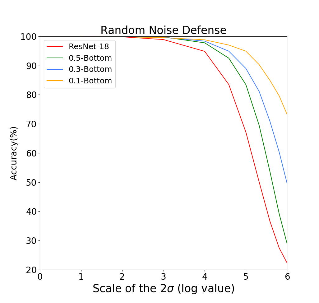
The experimental results are shown in Figure 4. The standard CNN is still robust to small scale Gaussian noise such as $\sigma\leq 8$. After that, the performance of the standard CNN begins to drop sharply as $\sigma$ increases. In contrast, defective CNNs show far better robustness than the standard version. The defective CNN with keep probability $0.1$ can maintain high accuracy until $\sigma$ increase to $16$ and have a much slower downward trend as $\sigma$ increases.

Figure 4: Defense performance against additive Gaussian noise. $p\text{-Bottom}$ means applying defective convolutional layers with keep probability $p$ to the bottom layers of a standard ResNet-18.

4.4 Ablation Studies

There are several design choices of the defective CNN, which include the appropriate positions to apply defective convolutional layers, the benefit of breaking symmetry, the diversity introduced by randomness, as well as the extensibility of defective layers via structure adjustment. In this subsection, we conduct a series of comparative experiments and use black-box defense performance against transfer-based attacks as the evaluation criterion. In our experiments, we found that the performance is not sensitive to the choices on the source model to attack and the target model to defense. Without loss of generality, we only list the performances using DenseNet-121 as the source model and ResNet-18 as the target model on the CIFAR-10 dataset and leave more experimental results in Appendix 0.A.7. The results are listed in Table 5.

Architecture	$\text{FGSM}_{16}$	$\text{PGD}_{16}$	$\text{PGD}_{32}$	$\text{CW}_{40}$	Test Accuracy
ResNet-18	14.91%	14.14%	7.16%	8.23%	95.33%
0.7-Bottom	23.29%	51.29%	37.00%	36.95%	94.03%
0.5-Bottom	30.86%	70.38%	56.36%	54.02%	93.39%
0.3-Bottom	48.57%	86.99%	78.41%	73.70%	91.83%
0.7-Top	14.62%	10.55%	4.91%	7.88%	95.16%
0.5-Top	10.76%	11.06%	5.10%	7.19%	94.94%
0.3-Top	11.23%	11.77%	5.80%	10.10%	94.61%
0.7-Bottom, 0.7-Top	24.15%	45.12%	30.24%	29.65%	94.16%
0.7-Bottom, 0.3-Top	11.26%	33.67%	20.28%	23.31%	93.44%
0.3-Bottom, 0.3-Top	27.43%	75.49%	62.78%	62.47%	89.78%
0.3-Bottom, 0.7-Top	40.58%	82.77%	72.15%	68.58%	91.23%
0.5-Bottom	30.86%	70.38%	56.36%	54.02%	93.39%
0.1-Bottom	79.93%	96.70%	94.68%	89.67%	87.68%
$\text{0.5-Bottom}_{\text{DC}}$	12.15%	19.93%	11.20%	12.72%	95.12%
$\text{0.1-Bottom}_{\text{DC}}$	19.00%	53.87%	41.40%	44.80%	93.27%
$\text{0.5-Bottom}_{\text{SM}}$	48.86%	85.00%	75.60%	72.07%	92.57%
$\text{0.1-Bottom}_{\text{SM}}$	39.40%	80.36%	72.43%	65.38%	74.28%
$\text{0.5-Bottom}_{\times 2}$	20.78%	50.16%	34.24%	34.00%	94.12%
$\text{0.1-Bottom}_{\times 2}$	68.83%	93.35%	88.25%	82.74%	90.49%

Table 5: Ablation experiments of defective CNNs. Numbers in the middle mean the success defense rates. $p\text{-Bottom}$ and $p\text{-Top}$ mean applying defective layers with keep probability $p$ to bottom layers and top layers respectively. $p\text{-Bottom}_{\text{DC}}$ means making whole channels defective with keep probability $p$. $p\text{-Bottom}_{\text{SM}}$ means using the same defective mask in every channel with keep probability $p$. $p\text{-Bottom}_{\times n}$ means increasing channel number to $n$ times at defective layers. $\text{FGSM}_{16}$, $\text{PGD}_{16}$ and $\text{PGD}_{32}$ denote attack method FGSM with perturbation scale $\ell_{\infty}=16$, PGD with perturbation scale $\ell_{\infty}=16$ and $32$ respectively. $\text{CW}_{40}$ denotes CW attack method [6] with confidence $\kappa=40$.

Defective Layers on Bottom layers v.s Top Layers. We apply defective layers with different keep probabilities to the bottom layers and the top layers of the original CNN, respectively. Comparing the results of the models with the same keep probability but different parts being masked, we find that applying defective layers to bottom layers enjoys significantly higher success defense rates. Moreover, only applying defective layers to bottom layers can achieve better performance than applying defective layers on both the bottom and top layers. The bottom layers mainly contribute to detect the edges and shape, while the receptive fields of neurons in top layers are too large to respond to the location sensitive information. This corroborates the phenomena shown in [47, 30]. Also, we find that the defense accuracy monotonically increases as the test accuracy decreases along with the keep probability (See the trend map in Appendix 0.A.6). The appropriate value for the keep probability mainly depends on the relative importance of generalization and robustness.

Defective Neuron v.s. Defective Channel. As our method independently selects defective neurons on different channels in a layer, we break the symmetry of the original CNN structure. To see whether this asymmetric structure would help, we try to directly mask whole channels instead of neurons using the same keep probability as the defective layer and train it to see the performance. This defective channel method does not hurt the symmetry while also leading to the same decrease in the number of convolutional operations. Table 5 shows that although our defective CNN suffers a small drop in test accuracy due to the low keep probability, we have a great gain in the robustness, compared with the defective-channel CNN.

Defective Masks are Shared Among Channels or Not. The randomness in generating masks in different channels and layers allows each convolutional filter to focus on different input patterns. Also, it naturally involves various topological structures for local feature extraction instead of learning [8, 7]. We show the essentiality of generating various masks per layer via experiments that compare to a method that only randomly generates one mask per layer and uses it in every channel. Table 5 shows that applying the same mask to each channel will decrease the test accuracy. This may result from the limitation of expressivity due to the monotone masks at every channel of the defective layer.

Increase the Number of Channels at Defective Layers. Although masking neurons does not reduce the parameters of the CNN, it reduces the number of convolutional operations and may decrease the expressive capacity of the CNN. To compensate for these defective positions, we increase the number of neurons at the defective layers by increasing the number of channels. Table 5 shows that increasing channels does help the network with defective layers to obtain higher test accuracy while maintaining good robustness performance.

5 Conclusion

In this paper, we introduce and experiment on defective CNNs, a modified version of existing CNNs that makes CNNs capture more information other than local textures, especially the shape. We show that defective CNNs can achieve much better robustness while maintaining high test accuracy. More specifically, by using defective convolutional layers, we reach state-of-the-art performance against two transfer-based attack methods. Another insight resulting from our experiments is that the adversarial perturbations generated against defective CNNs can actually change the semantic information of images and may even “fool” humans. We hope that these findings bring more understanding on adversarial examples and the robustness of neural networks.

Defective Convolutional Networks Supplementary Material

Table of Contents

• Appendix A: More Experimental Results

  • Transfer-based Attack from Ensemble Models on CIFAR-10

  • Transfer-based Attack on MNIST

  • Gray-box Attack

  • White-box Attack

  • Randomly Shuffled Images and Stylized-ImageNet

  • Black-box Attack with Different Keep Probabilities

  • Full Information on Experiments Mentioned in Section 4.3

• Appendix B: Adversarial Examples Generated by Defective CNNs

• Appendix C: Architecture Illustrations

• Appendix D: Training Details on CIFAR-10 and MNIST

• Appendix E: Attack approaches

Appendix 0.A More Experimental Results

0.A.1 Transfer-based Attack from Ensemble Models on CIFAR-10

In this subsection, we evaluate the defense performance of networks with defective convolutional layers against transfer-based attack from ensemble models on the CIFAR-10 dataset. We apply defective convolutional layers to five popular network architectures ResNet-18, ResNet-50 [15], DenseNet-121, SENet-18 [19], VGG-19 [36], and test the black-box defense performance against transfer-based attacks from ensemble models on the CIFAR-10 dataset. For each architecture, we replace the standard convolutional layer with the defective version on the bottom layers of different architectures. Illustrations of defective layers applied to these network architectures can be found in Appendix 0.C. We test the black-box defense performance against transfer-based attacks on 5000 samples from the validation set. Adversarial examples are generated by PGD, which runs for $7$ steps with step size $2$ and the $\ell_{\infty}$ perturbation scale is set to $8$. We generate five ensemble models as the source model by fusing every four models in all five models.

The results can be found in Table 6. These results show that defective convolutional layers can consistently improve the black-box defense performance of various network architectures against transfer-based attacks from ensemble models on the CIFAR-10 dataset.

Architecture	–ResNet-18	–ResNet-50	–DenseNet-121	–SENet-18	–VGG-19	Test Accuracy
ResNet-18	1.02%	0.74%	0.76%	0.94%	0.88%	95.33%
0.5-Bottom	32.98%	35.95%	29.36%	32.31%	37.24%	93.39%
0.3-Bottom	69.52%	72.44%	67.02%	68.63%	72.23%	91.83%
ResNet-50	1.07%	2.32%	1.31%	1.17%	0.82%	95.25%
0.5-Bottom	23.61%	31.52%	21.20%	22.89%	25.59%	94.43%
0.3-Bottom	55.47%	62.43%	53.25%	55.13%	58.47%	93.46%
DenseNet-121	0.70%	0.88%	1.37%	0.74%	0.58%	95.53%
0.5-Bottom	6.99%	10.19%	7.77%	6.93%	8.10%	94.34%
0.3-Bottom	32.07%	38.28%	31.59%	31.01%	35.42%	92.82%
SENet-18	0.91%	0.66%	0.74%	0.92%	0.64%	95.09%
0.5-Bottom	29.16%	32.58%	25.84%	29.17%	32.88%	93.53%
0.3-Bottom	62.12%	65.83%	59.94%	62.90%	65.64%	92.54%
VGG-19	8.27%	8.28%	6.42%	7.64%	14.08%	93.93%
0.5-Bottom	60.62%	63.71%	57.85%	59.28%	64.73%	91.73%
0.3-Bottom	80.97%	82.84%	80.06%	80.04%	82.86%	90.11%

Table 6: Black-box defense performances against transfer-based attacks from ensemble models on the CIFAR-10 dataset. Numbers in the middle mean the success defense rates. Networks in the first row indicate the source models which ensemble other four models except for the network itself. The source model generates adversarial examples by PGD. 0.5-Bottom and 0.3-Bottom mean applying defective convolutional layers with keep probability 0.5 and 0.3 to the bottom layers of the network whose name lies just above them. The source and target networks are initialized differently if they share the same architecture.

0.A.2 Transfer-based Attack on MNIST

In this subsection, we evaluate the defense performance of networks with defective convolutional layers against trasfer-based attack on the MINST dataset. We apply defective convolutional layers to five popular network architectures ResNet-18, ResNet-50, DenseNet-121, SENet-18, VGG-19, and test the black-box defense performance against transfer-based attacks on MNIST dataset. For each architecture, we replace the standard convolutional layer with the defective version on bottom layers of different architectures. Illustrations of defective layers applied to these network architectures can be found in Appendix 0.C. We test the black-box defense performance against transfer-based attacks on 5000 samples from the validation set. Adversarial examples are generated by PGD which runs for 40 steps with step size $0.01\times 255$ and perturbation scale $0.3\times 255$.

The results can be found in Table 7. These results show that defective convolutional layers can consistently improve the black-box defense performance of various network architectures against transfer-based attacks on the MNIST dataset.

Architecture	ResNet-18	ResNet-50	DenseNet-121	SENet-18	VGG-19	Test Accuracy
ResNet-18	0.06%	24.13%	1.66%	0.14%	9.57%	99.49%
0.5-Bottom	3.49%	43.04%	8.66%	7.66%	26.47%	99.34%
0.3-Bottom	25.91%	75.59%	36.19%	38.03%	64.63%	99.29%
ResNet-50	2.93%	9.30%	7.68%	5.94%	19.68%	99.39%
0.5-Bottom	8.54%	23.06%	8.76%	10.09%	28.49%	99.32%
0.3-Bottom	10.91%	36.44%	16.04%	14.55%	39.57%	99.28%
DenseNet-121	0.48%	29.81%	0.02%	1.64%	9.90%	99.48%
0.5-Bottom	2.57%	35.85%	1.10%	3.93%	16.29%	99.46%
0.3-Bottom	7.13%	58.92%	3.37%	11.39%	32.69%	99.38%
SENet-18	0.22%	18.77%	2.34%	0.10%	13.75%	99.41%
0.5-Bottom	3.37%	24.09%	6.90%	2.21%	17.24%	99.35%
0.3-Bottom	11.97%	51.63%	14.39%	16.45%	40.23%	99.31%
VGG-19	3.83%	51.77%	5.59%	7.34%	3.25%	99.48%
0.5-Bottom	12.47%	61.18%	12.91%	21.71%	19.32%	99.37%
0.3-Bottom	29.14%	70.59%	31.55%	41.87%	47.65%	99.33%

Table 7: Black-box defense performances against transfer-based attacks on the MNIST dataset. Numbers in the middle mean the success defense rates. Networks in the first row are the source models for generating adversarial examples by PGD. 0.5-Bottom and 0.3-Bottom mean applying defective convolutional layers with keep probability 0.5 and 0.3 to the bottom layers of the network whose name lies just above them. The source and target networks are initialized differently if they share the same architecture.

0.A.3 Gray-box Attack

In this subsection, we show the gray-box defense performance of defective CNNs on the CIFAR-10 dataset. We use gray-box attacks in the following two ways. One way is to generate adversarial examples against one trained neural network and test those images on a network with the same structure but different initializations. The other way is specific to our defective models. We generate adversarial examples on one trained defective CNN and test them on a network with the same keep probability but different sampling of defective neurons. In both of these two ways, the adversarial knows some information on the structure of the network but does not know the specific parameters of it.

Architecture	0.5-Bottom	0.3-Bottom
0.5-Bottom	30.90%	40.49%
$\text{0.5-Bottom}_{\text{DIF}}$	32.77%	40.39%
0.3-Bottom	59.24%	36.84%
$\text{0.3-Bottom}_{\text{DIF}}$	57.45%	37.04%

Table 8: Defense performances against two kinds of gray-box attacks for defective CNNs. Numbers mean the success defense rates. Networks in the first row are the source models for generating adversarial examples by PGD, which runs for $20$ steps with step size $1$ and perturbation scale $\ell_{\infty}=16$. 0.5-Bottom and 0.3-Bottom in the left column represent the networks with the same structure as the corresponding source networks but with different initialization. $\text{0.5-Bottom}_{\text{DIF}}$ and $\text{0.3-Bottom}_{\text{DIF}}$ in the left column represent the networks with the same keep probabilities as the corresponding source networks but with different sampling of defective neurons.

From the results listed in Table 8, we find that defective CNNs have similar performance on adversarial examples generated by our two kinds of gray-box attacks. This phenomenon indicates that defective CNNs with the same keep probability would catch similar information which is insensitive to the selections of defective neurons. Also, comparing with the gray-box performance of standard CNNs (See Table 9), defective CNNs show stronger defense ability.

Architecture	ResNet-18	DenseNet-121
ResNet-18	5.98%	14.14%
DenseNet-121	14.53%	2.98%

Table 9: Defense performances against gray-box attacks for standard CNNs. Numbers mean the success defense rates. Networks in the first row are the source models for generating adversarial examples by PGD, which runs for $20$ steps with step size $1$ and perturbation scale $\ell_{\infty}=16$. The diagonal shows gray-box performances in the setting that the source and target networks share the same structure but with different initializations.

0.A.4 White-box Attack

In this subsection, we show the white-box defense performance of defective CNNs. Table 10 shows the results of ResNet-18 on the CIFAR-10 dataset. The performance on other network architectures is similar. Note that, the proposed method would not involve any obfuscated gradients [1]. Also, We study the combination of the proposed method and adversarial training. We adversarially train a defective CNN under the same setting described in [29] and reach 51.6% successful defense rate against the default PGD attack ($\ell_{\infty}=8$ and $7$ steps) used in training, which outperforms the standard CNN (50.0%).

We want to emphasize that the adversarial examples generated by defective CNNs appear to have semantic shapes and may even fool humans as well (see Figure 3 and Appendix 0.B). This indicates that small perturbations can actually change the semantic meaning of images for humans. Those samples should probably not be categorized into adversarial examples and used to evaluate white-box robustness. This is also aligned with [22].

To further verify the adversarial examples generated by defective CNNs align better with human perception than standard CNNs, we conduct a user study. We show users a pair of adversarial examples generated by defective CNNs and standard CNNs, respectively. The corresponding labels are attached. The user will be asked which one of the pair is better aligned with the predicted label. More specifically, we generate two sets of adversarial examples on CIFAR-10 and Tiny-ImageNet by defective CNNs and standard CNNs, respectively. For each user, we randomly sample $50$ pairs from the two sets and ask him/her to select. A total of $13$ people are involved in our study. The results show that all users select more images generated by defective CNNs than the ones generated by standard CNNs. On average, the number of defective CNNs ones is $14$ more than the number of standard CNNs ones. This supports our arguments.

Architecture	$\text{FGSM}_{1}$	$\text{FGSM}_{2}$	$\text{FGSM}_{4}$	$\text{PGD}_{2}$	$\text{PGD}_{4}$	$\text{PGD}_{8}$	Test Accuracy
ResNet-18	81.24%	65.78%	51.24%	23.80%	3.16%	0.02%	95.33%
0.5-Bottom	85.22%	68.65%	52.04%	38.16%	6.67%	0.12%	93.39%
0.3-Bottom	85.70%	69.69%	54.51%	49.01%	18.93%	2.86%	91.83%

Table 10: Defense performances against white-box attacks. Numbers in the middle mean the success defense rates. $\text{FGSM}_{1},\text{FGSM}_{2},\text{FGSM}_{4}$ refer to FGSM with perturbation scale 1,2,4 respectively. $\text{PGD}_{2},\text{PGD}_{4},\text{PGD}_{8}$ refer to PGD with perturbation scale 2,4,8 and step number 4,6,10 respectively. The step size of all PGD methods are set to 1.

0.A.5 Randomly Shuffled Images and Stylized-ImageNet

In this subsection, we show more results on randomly shuffled images and Stylized-ImageNet [12]. As shown in Section 3.2, shape information in randomly shuffled images is destroyed while textural information preserving, and Stylized-ImageNet has the opposite situation. If a CNN make predictions relying less on textural information but more on shape information, it should have worse performance on randomly shuffled images but better performance on Stylized-ImageNet.

We construct defective CNNs by applying defective convolutional layers to the bottom layers of standard ResNet-18, ResNet-50, DenseNet-121, SENet-18, and VGG-19. We train all defective CNNs and their plain counterparts on the ImageNet dataset. For each pair of CNNs, we sample images from the validation set, which are predicted correctly by both two kinds of CNNs. We make manipulations to the sampled images by setting $k\in\{2,4,8\}$ and pick corresponding images from Stylized-ImageNet. We check the accuracy of all models on the these images. The results are shown in Table 11. We can see the defective CNNs perform consistently worse than the standard CNNs on the randomly shuffled images, and perform consistently better than the standard CNNs on Stylized-ImageNet. This justifies our argument that defective CNNs make predictions relying less on textural information but more on shape information.

Model	$2\times 2$	$4\times 4$	$8\times 8$	IN $\rightarrow$ SIN
ResNet-18	99.53%	84.36%	20.08%	15.33%
0.1-Bottom	96.32%	56.91%	9.04%	20.20%
ResNet-50	99.80%	87.34%	18.00%	15.12%
0.1-Bottom	98.30%	65.87%	9.23%	21.16%
DenseNet-121	99.55%	85.87%	18.78%	15.53%
0.1-Bottom	92.23%	47.82%	7.52%	19.09%
SENet-18	98.88%	75.57%	14.61%	15.83%
0.1-Bottom	92.39%	46.94%	7.07%	18.79%
VGG-19	99.10%	81.58%	15.45%	6.17%
0.1-Bottom	97.98%	71.85%	11.00%	13.98%

Table 11: The left three columns are the accuracy of classifying randomly shuffled test images. The rightmost column is the accuracy of training on ImageNet and testing on Stylized-ImageNet. 0.1-Bottom mean applying defective convolutional layers with keep probability 0.1 to the bottom layers of the network whose name lies just above them.

0.A.6 Black-box Attack with Different Keep Probabilities

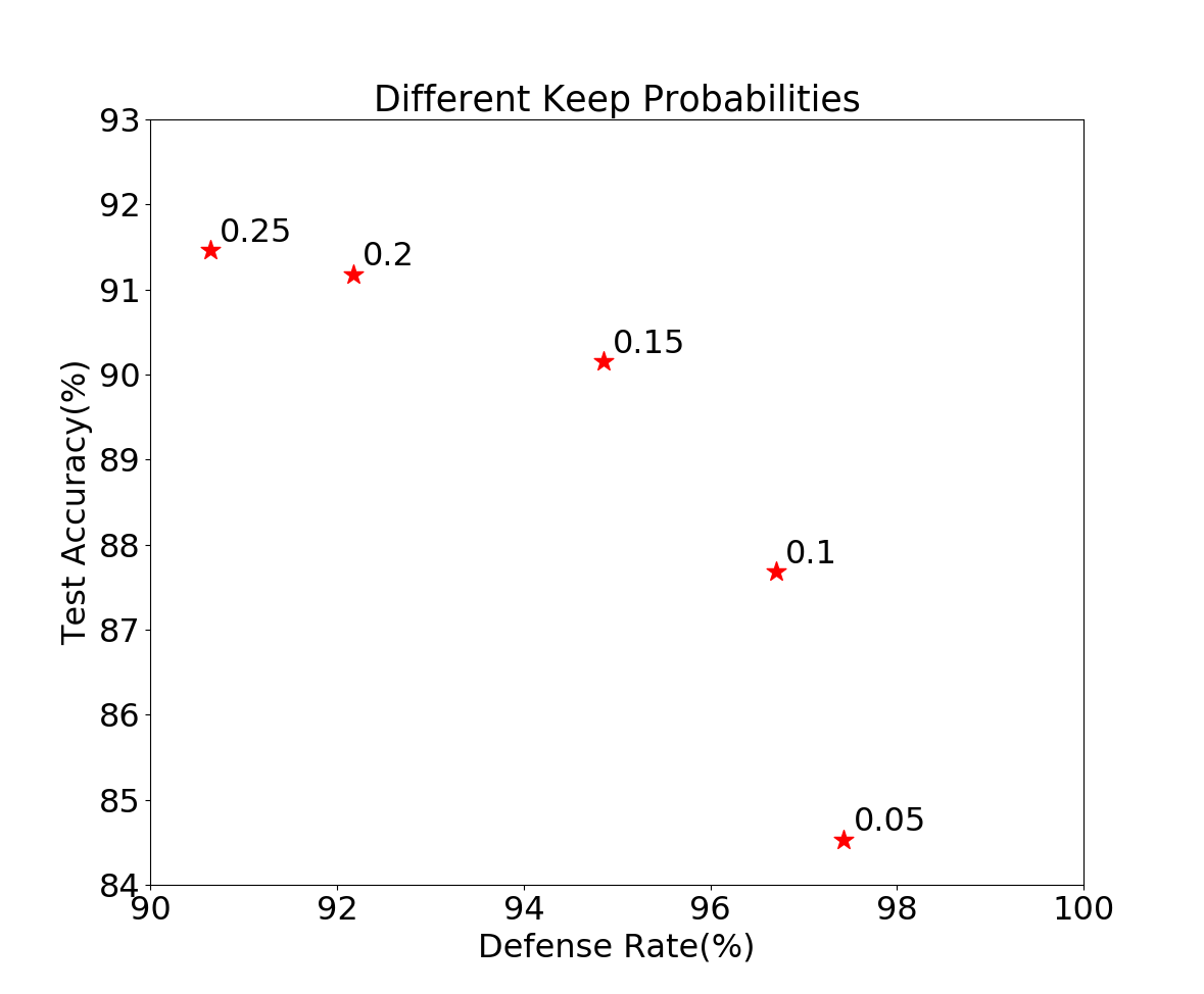
In this subsection, we show the trade-off between robustness and generalization performance in defective CNNs with different keep probabilities. We use DenseNet-121 [20] as the source model to generate adversarial examples from CIFAR-10 with PGD [23], which runs for 20 steps with step size 1 and perturbation scale 16. The defective convolutional layers are applied to the bottom layers of ResNet-18 [15]. Figure 5 shows that the defense accuracy monotonically increases as the test accuracy decreases along with the keep probability. We can see the trade-off between robustness and generalization.

Figure 5: Relationship between success defense rates against adversarial examples generated by PGD and test accuracy with respect to different keep probabilities. Each red star represents a specific keep probability with its value written near the star.

0.A.7 Full Information on Experiments Mentioned in Section 4.3

In this subsection, we will show more experimental results on defective CNNs using different adversarial examples, different attack methods and different mask settings on ResNet-18. The networks used to generate adversarial examples including ResNet-18, ResNet-50, DenseNet-121, SENet18, and VGG-19. More specifically, we choose $5000$ samples to generate adversarial examples via FGSM and PGD, and $1000$ samples for CW attack. All samples are drawn from the validation set of CIFAR-10 dataset and can be correctly classified correctly by the model used to generate adversarial examples.

For FGSM, we try step size $\epsilon\in\{8,16,32\}$, namely $\textbf{FGSM}_{8}$, $\textbf{FGSM}_{16}$, $\textbf{FGSM}_{32}$, to generate adversarial examples. For PGD, we have tried more extensive settings. Let $\{\epsilon,T,\alpha\}$ be the PGD setting with step size $\epsilon$, the number of steps $T$ and the perturbation scale $\alpha$, then we have tried PGD settings $(1,8,4),(2,4,4),(4,2,4),(1,12,8),(2,6,8),(4,3,8),(1,20,16),(2,10,16),(4,5,16),$ $(1,40,32),$ $(2,20,32),(4,10,32)$ to generate PGD adversarial examples. From the experimental results, we observe the following phenomena. First, we find that the larger the perturbation scale is, the stronger the adversarial examples are. Second, for a fixed perturbation scale, the smaller the step size is, the more successful the attack is, as it searches the adversarial examples in a more careful way around the original image. Based on these observation, we only show strong PGD attack results in the Appendix, namely the settings $(1,20,16)$ ($\textbf{PGD}_{16}$), $(2,10,16)$ ($\textbf{PGD}_{2,16}$) and $(1,40,32)$ ($\textbf{PGD}_{32}$). Nonetheless, our models also perform much better on weak PGD attacks. For the CW attack, we have also tried different confidence parameters $\kappa$. However, we find that for large $\kappa$, the algorithm is hard to find adversarial examples for some neural networks such as VGG because of its logit scale. For smaller $\kappa$, the adversarial examples have weak transferability, which means they can be easily defended even by standard CNNs. Therefore, in order to balance these two factors, we choose $\kappa=40$ ($\textbf{CW}_{40}$) for DenseNet-121, ResNet-50, SENet-18 and $\kappa=20$ ($\textbf{CW}_{20}$) for ResNet-18 as a good choice to compare our models with standard ones. The step number for choosing the parameter $c$ is set to $30$.

Note that the noises of FGSM and PGD are considered in the sense of $\ell_{\infty}$ norm and the noise of CW is considered in the sense of $\ell_{2}$ norm. All adversarial examples used to evaluate can fool the original network. Table 12,13,14,15 and 16 list our experimental results. DC means we replace defective neurons with defective channels in the corresponding blocks to achieve the same keep probability. SM means we use the same defective mask on all the channels in a layer. $\times n$ means we multiply the number of the channels in the defective blocks by $n$ times. EN means we ensemble five models with different defective masks of the same keep probability.

Appendix 0.B Adversarial Examples Generated by Defective CNNs

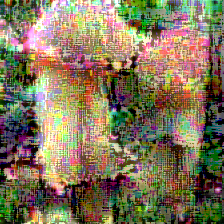
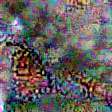
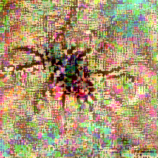
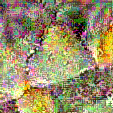
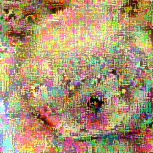
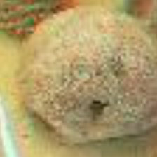
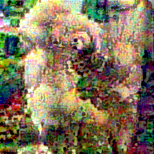
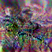
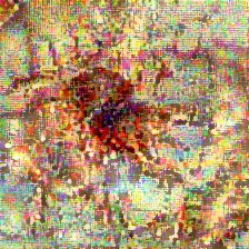
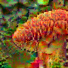
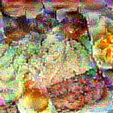
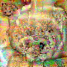
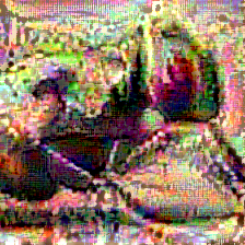
In this subsection, we show more adversarial examples generated by defective CNNs. Figure 6 shows some adversarial examples generated on the CIFAR-10 dataset along with the corresponding original images. These examples are generated from CIFAR-10 against a defective ResNet-18 of keep probability $0.2$ on the $0^{\text{th}},1^{\text{st}},2^{\text{nd}}$ blocks, a defective ResNet-18 of keep probability $0.1$ on the $1^{\text{st}},2^{\text{nd}}$ blocks, and a standard ResNet-18. We use attack method MIFGSM with perturbation scale $\alpha=16$ and $\alpha=32$. We also show some adversarial examples generated from Tiny-ImageNet along with the corresponding original images in Figure 7. These examples are generated from Tiny-ImageNet against a defective ResNet-18 of keep probability of the keep probability $0.1$ on the $1^{\text{st}},2^{\text{nd}}$ blocks and a standard ResNet-18. The attack methods are MIFGSM with scale $64$ and $32$, step size $1$ and step number $40$ and $80$ respectively.

The adversarial examples generated by defective CNNs exhibit more semantic shapes of their fooled classes, such as the mouth of the frog in Figure 6. This also corroborates the point made in [43] that more robust models will be more aligned with human perception.

(a) Frog

(b) Dog

(c) Automobile

(d) Dog

(e) Ship

(f) Dog

(g) Ship

(h) Bird

(i) Frog

(j) Truck

(k) Horse

(l) Truck

(m) Airplane

(n) Automobile

(o) Bird

(p) Automobile

(q) Ship

(r) Bird

(s) Frog

(t) Cat

(u) Automobile

(v) Dog

(w) Truck

(x) Plane

(y) Truck

(z) Plane

(aa) Deer

Figure 6: CIFAR-10 dataset. First row: the adversarial examples generated by defective CNNs and the predicted labels. Second row: original images. Second row: the adversarial examples generated by the standard CNN and the predicted labels.

(a) Mushroom

(b) Monarch Butterfly

(c) Black Widow

(d) Mushroom

(e) Sulphur Butterfly

(f) Teddy

(g) Ladybug

(h) Tarantula

(i) Black Widow

(j) Ladybug

(k) Goldfish

(l) Egyptian Cat

(m) Brain Coral

(n) Fly

(o) Standard Poodle

(p) Dragonfly

(q) Roach

(r) Mushroom

(s) Mashed Potato

(t) Teddy

(u) drumstick

Figure 7: Tiny-ImageNet dataset. First row: the adversarial examples generated by defective CNNs and the predicted labels. Second row: original images. Second row: the adversarial examples generated by the standard CNN and the predicted labels.

Appendix 0.C Architecture Illustrations

In this subsection, we briefly introduce the network architectures used in our experiments. Generally, we apply defective convolutional layers to the bottom layers of the networks and we have tried six different architectures, namely ResNet-18, ResNet-50, DenseNet-121, SENet-18, VGG-19 and WideResNet-32. We next illustrate these architectures and show how we apply defective convolutional layers to them. In our experiments, applying defective convolutional layers to a block means randomly selecting defective neurons in every layer of the block.

0.C.1 ResNet-18

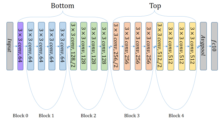
ResNet-18 [15] contains $5$ blocks: the $0^{\text{th}}$ block is one single $3\times 3$ convolutional layer, and each of the rest contains four $3\times 3$ convolutional layers. Figure 8 shows the whole structure of ResNet-18. In our experiments, we apply defective convolutional layers to the $0^{\text{th}},1^{\text{st}},2^{\text{nd}}$ blocks which are the bottom layers.

Figure 8: The architecture of ResNet-18

0.C.2 ResNet-50

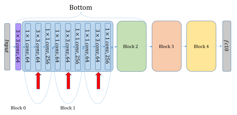
Similar to ResNet-18, ResNet-50 [15] contains $5$ blocks and each block contains several $1\times 1$ and $3\times 3$ convolutional layers (i.e. Bottlenecks). In our experiment, we apply defective convolutional layers to the $3\times 3$ convolutional layers in the first three “bottom” blocks. The defective layers in the $1^{\text{st}}$ block are marked by the red arrows in Figure 9.

Figure 9: The architecture of ResNet-50

0.C.3 DenseNet-121

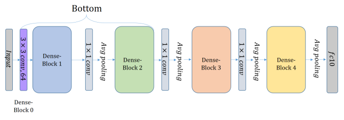
DenseNet-121 [20] is another popular network architecture in deep learning researches. Figure 10 shows the whole structure of DenseNet-121. It contains $5$ Dense-Blocks, each of which contains several $1\times 1$ and $3\times 3$ convolutional layers. Similar to what we do for ResNet-50, we apply defective convolutional layers to the $3\times 3$ convolutional layers in the first three “bottom” blocks. The growth rate is set to 32 in our experiments. vspace-0.1in

Figure 10: The architecture of DenseNet-121

0.C.4 SENet-18

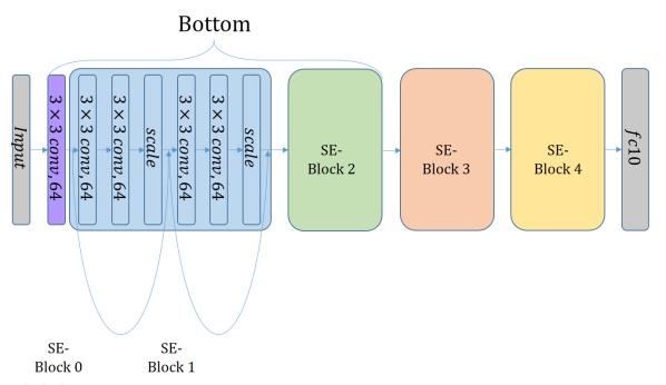
SENet [19], a network architecture which won the first place in ImageNet contest $2017$, is shown in Figure 11. Note that here we use the pre-activation shortcut version of SENet-18 and we apply defective convolutional layers to the convolutional layers in the first $3$ SE-blocks.

Figure 11: The architecture of SENet-18

0.C.5 VGG-19

VGG-19 [36] is a typical neural network architecture with sixteen $3\times 3$ convolutional layers and three fully-connected layers. We slightly modified the architecture by replacing the final $3$ fully connected layers with $1$ fully connected layer as is suggested by recent architectures. Figure 12 shows the whole structure of VGG-19. We apply defective convolutional layers on the first four $3\times 3$ convolutional layers.

Figure 12: The architecture of VGG-19

0.C.6 WideResNet-32

Based on residual networks, [46] proposed a wide version of residual networks which have much more channels. In our experiments, we adopt the network with a width factor of $4$ and apply defective layers on the $0^{\text{th}}$ and $1^{\text{st}}$ blocks. Figure 13 shows the whole structure of WideResNet-32.

Figure 13: The architecture of WideResNet-32

Appendix 0.D Training Details on CIFAR-10 and MNIST

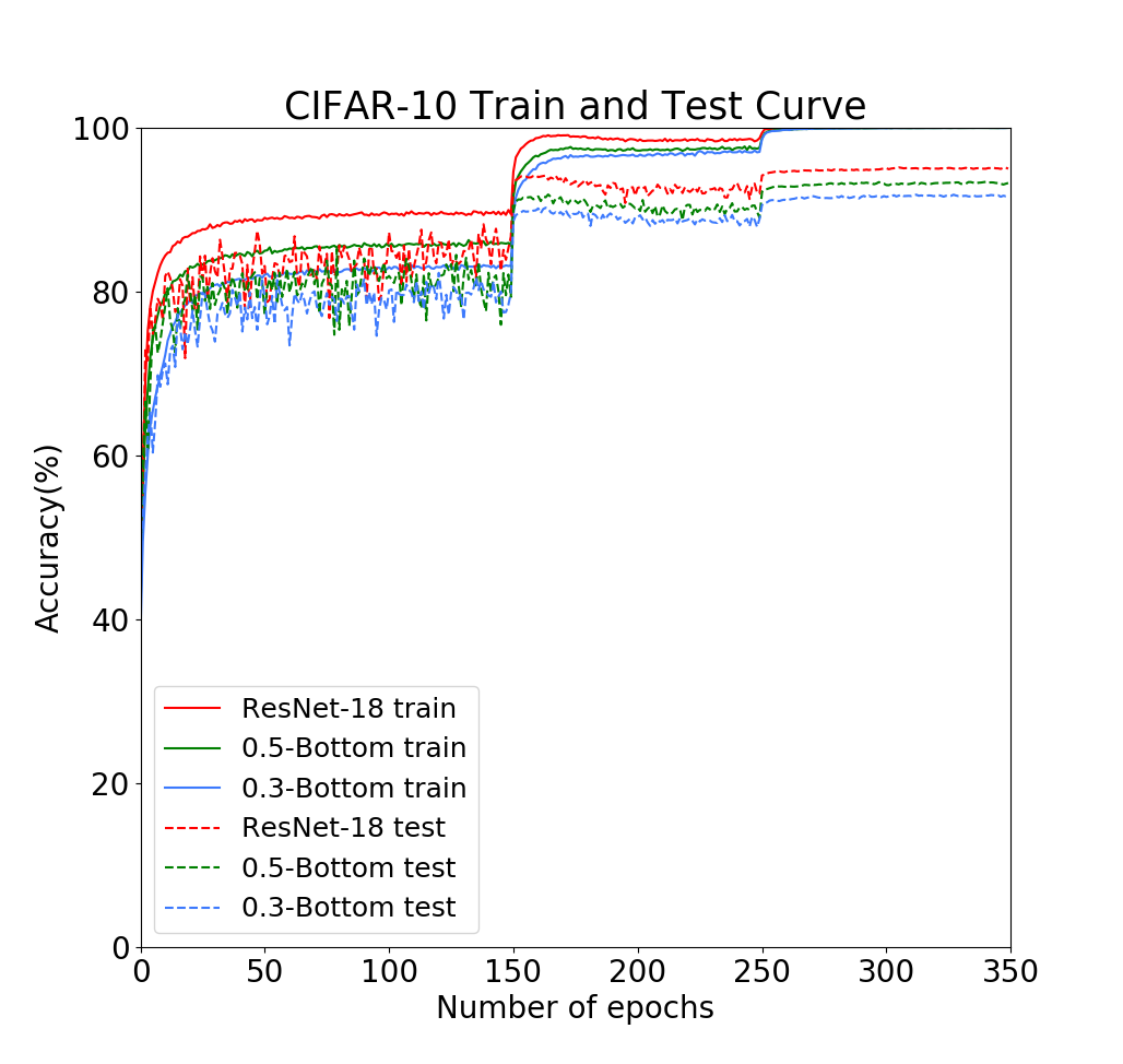
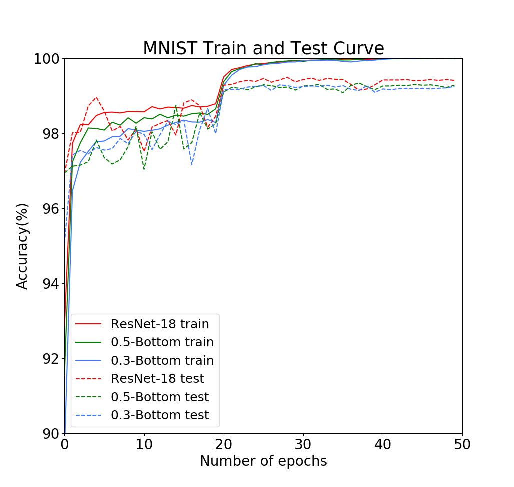
To guarantee our experiments are reproducible, here we present more details on the training process in our experiments. When training models on CIFAR-10, we first subtract per-pixel mean. Then we apply a zero-padding of width $4$, a random horizontal flip and a random crop of size $32\times 32$ on train data. No other data augmentation method is used. We apply SGD with momentum parameter $0.9$, weight decay parameter $5\times 10^{-4}$ and mini-batch size $128$ to train on the data for $350$ epochs. The learning rate starts from $0.1$ and is divided by 10 when the number of epochs reaches $150$ and $250$. When training models on MNIST, we first subtract per-pixel mean. Then we apply random horizontal flip on train data. We apply SGD with momentum parameter $0.9$, weight decay parameter $5\times 10^{-4}$ and mini-batch size $128$ to train on the data for $50$ epochs. The learning rate starts from $0.1$ and is divided by 10 when the number of epochs reaches $20$ and $40$. Figure 14 shows the train and test curves of standard and defective ResNet-18 on CIFAR-10 and MNIST. Different network structures share similar tendency regarding the train and test curves.

(a) CIFAR-10

(b) MNIST

Figure 14: Train and test curve of standard and defective ResNet-18 on CIFAR-10 and MNIST

Appendix 0.E Attack approaches

In this subsection, we describe the attack approaches used in our experiments. We first give an overview of how to attack a neural network in mathematical notations. Let ${\bm{x}}$ be the input to the neural network and $f_{\bm{\theta}}$ be the function which represents the neural network with parameter ${\bm{\theta}}$. The output label of the network to the input can be computed as $c=\operatorname*{arg\,max}_{i}f_{\bm{\theta}}({\bm{x}})_{i}$. In order to perform an adversarial attack, we add a small perturbation $\mathbf{\delta}_{x}$ to the original image and get an adversarial image ${\bm{x}}_{\text{adv}}={\bm{x}}+\mathbf{\delta}_{x}$. The new input ${\bm{x}}_{\text{adv}}$ should look visually similar to the original ${\bm{x}}$. Here we use the commonly used $\ell_{\infty}$-norm metric to measure similarity, i.e., we require that $||\mathbf{\delta}_{x}||\leq\epsilon$. The attack is considered successful if the predicted label of the perturbed image $c_{\text{adv}}=\operatorname*{arg\,max}_{i}f_{\bm{\theta}}({\bm{x}}_{\text{adv}})_{i}$ is different from $c$.

Generally speaking, there are two types of attack methods: Targeted Attack, which aims to change the output label of an image to a specific (and different) one, and Untargeted Attack, which only aims to change the output label and does not restrict which specific label the modified example should let the network output.

In this paper, we mainly use the following four gradient-based attack approaches. $J$ denotes the loss function of the neural network and $y$ denotes the ground truth label of ${\bm{x}}$.

• Fast Gradient Sign Method (FGSM). FGSM  [14] is a one-step untargeted method which generates the adversarial example ${\bm{x}}_{\text{adv}}$ by adding the sign of the gradients multiplied by a step size $\epsilon$ to the original benign image ${\bm{x}}$. Note that FGSM controls the $\ell_{\infty}$-norm between the adversarial example and the original one by the parameter $\epsilon$.

  $${\bm{x}}_{\text{adv}}={\bm{x}}+\epsilon\cdot\text{sign}(\nabla_{\bm{x}}J({\bm{x}},y)).$$

• Basic iterative method (PGD). PGD [23] is a multiple-step attack method which applies FGSM multiple times. To make the adversarial example still stay “close” to the original image, the image is projected to the $\ell_{\infty}$-ball centered at the original image after every step. The radius of the $\ell_{\infty}$-ball is called perturbation scale and is denoted by $\alpha$.

  $${\bm{x}}_{\text{adv}}^{0}={\bm{x}},\;\;\;{\bm{x}}_{\text{adv}}^{k+1}=\text{Clip}_{{\bm{x}},\alpha}\left[{\bm{x}}_{\text{adv}}^{k}+\epsilon\cdot\text{sign}(\nabla_{{\bm{x}}}J({\bm{x}}_{\text{adv}}^{k},y))\right].$$

• Momentum Iterative Fast Gradient Sign Method (MIFGSM).
  MIFGSM [9] is a recently proposed multiple-step attack method. It is similar to PGD, but it computes the optimize direction by a momentum instead of the gradients. The radius of the $\ell_{\infty}$-ball is also called perturbation scale and is denoted by $\alpha$.

  $$g_{k+1}=\mu\cdot g_{k}+\frac{\nabla_{{\bm{x}}}J({\bm{x}}_{\text{adv}}^{k},y)}{\|\nabla_{{\bm{x}}}J({\bm{x}}_{\text{adv}}^{k},y)\|_{1}}$$

  $${\bm{x}}_{\text{adv}}^{0}={\bm{x}},g_{0}=0\;\;\;{\bm{x}}_{\text{adv}}^{k+1}=\text{Clip}_{{\bm{x}},\alpha}\left[{\bm{x}}_{\text{adv}}^{k}+\epsilon\cdot\text{sign}(g_{k+1})\right].$$

• CW Attack. [6] shows that constructing an adversarial example can be formulated as solving the following optimization problem:

  $${\bm{x}}_{\text{adv}}=\operatorname*{arg\,min}_{{\bm{x}}^{\prime}}c\cdot g({\bm{x}}^{\prime})+||{\bm{x}}^{\prime}-{\bm{x}}||_{2}^{2},$$

  where $c\cdot g({\bm{x}}^{\prime})$ is the loss function that evaluates the quality of ${\bm{x}}^{\prime}$ as an adversarial example and the term $||{\bm{x}}^{\prime}-{\bm{x}}||_{2}^{2}$ controls the scale of the perturbation. More specifically, in the untargeted attack setting, the loss function $g({\bm{x}})$ can be defined as below, where the parameter $\kappa$ is called confidence.

  $$g({\bm{x}})=\max\{\max_{i\neq y}\left(f({\bm{x}})_{i}\right)-f({\bm{x}})_{y},-\kappa\},$$

Architecture	$\text{FGSM}_{8}$	$\text{FGSM}_{16}$	$\text{FGSM}_{32}$	$\text{PGD}_{16}$	$\text{PGD}_{2,16}$	$\text{PGD}_{32}$	$\text{CW}_{40}$	Acc
ResNet-18	29.78%	14.91%	11.53%	14.14%	10.02%	7.16%	8.23%	95.33%
0.7-Bottom	55.40%	23.29%	7.73%	51.29%	42.44%	37.00%	36.95%	94.03%
0.5-Bottom	66.87%	30.86%	6.65%	70.38%	62.11%	56.36%	54.02%	93.39%
0.3-Bottom	79.50%	48.57%	10.51%	86.99%	81.78%	78.41%	73.70%	91.83%
0.25-Bottom	83.12%	59.22%	17.16%	90.64%	86.22%	83.86%	77.82%	91.46%
0.2-Bottom	85.49%	63.01%	15.57%	92.17%	88.72%	86.50%	81.75%	91.18%
0.15-Bottom	88.18%	65.27%	18.33%	94.85%	92.24%	90.64%	85.46%	90.15%
0.1-Bottom	94.08%	79.93%	43.70%	96.70%	95.69%	94.68%	89.67%	87.68%
0.05-Bottom	96.16%	87.36%	59.05%	97.43%	97.13%	96.24%	90.24%	84.53%
0.7-Top	28.51%	14.62%	8.78%	10.55%	7.22%	4.91%	7.88%	95.16%
0.5-Top	25.01%	10.76%	10.24%	11.06%	7.99%	5.10%	7.19%	94.94%
0.3-Top	23.94%	11.23%	10.48%	11.77%	8.83%	5.80%	10.10%	94.61%
0.5-Bottom, 0.5-Top	55.88%	20.77%	9.96%	60.75%	51.47%	45.29%	47.32%	92.48%
0.7-Bottom, 0.7-Top	51.03%	24.15%	10.82%	45.12%	35.70%	30.24%	29.65%	94.16%
0.7-Bottom, 0.3-Top	36.16%	11.26%	9.16%	33.67%	24.62%	20.28%	23.31%	93.44%
0.3-Bottom, 0.3-Top	64.85%	27.43%	10.09%	75.49%	67.09%	62.78%	62.47%	89.78%
0.3-Bottom, 0.7-Top	74.73%	40.58%	9.12%	82.77%	75.98%	72.15%	68.58%	91.23%
$\text{0.5-Bottom}_{\text{DC}}$	36.39%	12.15%	8.24%	19.93%	14.99%	11.20%	12.72%	95.12%
$\text{0.3-Bottom}_{\text{DC}}$	43.81%	17.74%	8.32%	27.47%	21.73%	16.59%	19.34%	94.23%
$\text{0.1-Bottom}_{\text{DC}}$	49.53%	19.00%	7.23%	53.87%	44.78%	41.40%	44.80%	93.27%
$\text{0.5-Bottom}_{\text{SM}}$	77.30%	48.86%	12.50%	85.00%	80.01%	75.60%	72.07%	92.57%
$\text{0.3-Bottom}_{\text{SM}}$	82.59%	48.03%	12.30%	91.01%	87.35%	84.71%	79.55%	89.81%
$\text{0.1-Bottom}_{\text{SM}}$	67.06%	39.40%	16.25%	80.36%	74.97%	72.43%	65.38%	74.28%
$\text{0.5-Bottom}_{\times 2}$	51.25%	20.78%	10.29%	50.16%	40.47%	34.24%	34.00%	94.12%
$\text{0.3-Bottom}_{\times 2}$	68.82%	30.94%	7.22%	76.62%	67.90%	62.87%	60.17%	93.01%
$\text{0.1-Bottom}_{\times 2}$	88.00%	68.83%	28.55%	93.35%	90.82%	88.25%	82.74%	90.49%
$\text{ ResNet-18}_{\text{EN}}$	34.98%	16.51%	10.32%	12.60%	9.22%	5.48%	8.46%	96.03%
$\text{0.5-Bottom}_{\times 2,\text{EN}}$	58.49%	20.75%	8.48%	57.47%	47.05%	39.21%	41.36%	95.10%
$\text{0.5-Bottom}_{\text{EN}}$	69.35%	31.38%	7.73%	75.40%	66.37%	60.59%	58.07%	94.56%
$\text{0.3-Bottom}_{\text{EN}}$	81.98%	51.81%	8.57%	90.00%	85.25%	82.15%	77.74%	93.31%
$\text{0.1-Bottom}_{\text{EN}}$	95.37%	81.95%	43.42%	97.91%	97.10%	95.90%	91.36%	89.45%

Table 12: Extended experimental results of Section 4.3. Adversarial examples generated against DenseNet-121. Numbers in the middle mean the success defense rates. The model trained on CIFAR-10 achieves 95.62% accuracy on test set. $p\text{-Bottom},p\text{-Top},p\text{-Bottom}_{\text{DC}}$, $p\text{-Bottom}_{\text{SM}}$, $p\text{-Bottom}_{\times n}$ and $p\text{-Bottom}_{\text{EN}}$ mean applying defective layers with keep probability $p$ to bottom layers, applying defective layers with keep probability $p$ to top layers, making whole channels defective with keep probability $p$, using the same defective mask in every channel with keep probability $p$, increasing channel number to $n$ times at bottom layers and ensemble five models with different defective masks of the same keep probability $p$ respectively.

Architecture	$\text{FGSM}_{8}$	$\text{FGSM}_{16}$	$\text{FGSM}_{32}$	$\text{PGD}_{16}$	$\text{PGD}_{2,16}$	$\text{PGD}_{32}$	$\text{CW}_{20}$	Acc
ResNet-18	26.99%	13.91%	3.57%	5.98%	3.70%	3.02%	2.19%	95.33%
0.7-Bottom	48.76%	21.32%	9.54%	34.43%	25.14%	24.16%	38.87%	94.03%
0.5-Bottom	59.66%	30.48%	11.60%	53.89%	45.47%	41.27%	60.65%	93.39%
0.3-Bottom	74.00%	47.11%	15.65%	78.23%	73.30%	65.83%	79.04%	91.83%
0.25-Bottom	78.37%	56.05%	21.44%	83.96%	80.09%	73.45%	81.59%	91.46%
0.2-Bottom	81.67%	59.14%	19.60%	88.18%	85.07%	78.72%	82.78%	91.18%
0.15-Bottom	86.31%	63.16%	22.23%	92.26%	89.99%	85.14%	86.06%	90.15%
0.1-Bottom	92.89%	77.90%	45.63%	96.27%	95.30%	92.80%	90.29%	87.68%
0.05-Bottom	95.07%	85.40%	59.91%	97.51%	96.69%	95.30%	90.97%	84.53%
0.7-Top	25.96%	15.46%	7.18%	5.36%	2.83%	2.89%	2.66%	95.16%
0.5-Top	25.21%	9.21%	1.44%	5.98%	4.30%	3.25%	3.15%	94.94%
0.3-Top	24.36%	9.49%	2.60%	8.54%	5.30%	5.02%	6.62%	94.61%
0.5-Bottom, 0.5-Top	51.89%	20.41%	10.75%	45.99%	37.78%	34.09%	52.11%	92.48%
0.7-Bottom, 0.7-Top	43.32%	20.55%	4.14%	29.28%	19.64%	20.14%	32.92%	94.16%
0.7-Bottom, 0.3-Top	34.09%	11.05%	1.58%	23.06%	15.26%	14.93%	24.11%	93.44%
0.3-Bottom, 0.3-Top	61.22%	28.11%	13.78%	67.30%	59.43%	52.95%	69.15%	89.78%
0.3-Bottom, 0.7-Top	70.43%	39.15%	13.94%	74.85%	68.23%	62.52%	74.57%	91.23%
$\text{0.5-Bottom}_{\text{DC}}$	32.86%	13.89%	3.71%	9.41%	5.60%	5.34%	6.10%	95.12%
$\text{0.3-Bottom}_{\text{DC}}$	37.96%	16.23%	5.05%	16.63%	11.49%	10.54%	15.44%	94.23%
$\text{0.1-Bottom}_{\text{DC}}$	48.54%	19.10%	11.37%	41.14%	31.82%	30.56%	50.62%	93.27%
$\text{0.5-Bottom}_{\text{SM}}$	73.96%	47.63%	16.60%	75.60%	68.88%	62.10%	73.68%	92.57%
$\text{0.3-Bottom}_{\text{SM}}$	80.80%	48.37%	15.26%	87.88%	84.37%	77.69%	82.34%	89.81%
$\text{0.1-Bottom}_{\text{SM}}$	69.15%	43.55%	20.26%	79.96%	75.52%	71.95%	71.62%	74.28%
$\text{0.5-Bottom}_{\times 2}$	46.50%	21.37%	6.06%	32.98%	22.90%	22.66%	39.12%	94.12%
$\text{0.3-Bottom}_{\times 2}$	63.37%	29.90%	12.07%	61.81%	53.25%	48.36%	67.02%	93.01%
$\text{0.1-Bottom}_{\times 2}$	84.28%	64.47%	31.90%	90.76%	87.81%	82.61%	85.08%	90.49%
$\text{ ResNet-18}_{\text{EN}}$	29.36%	13.89%	3.81%	4.72%	2.88%	2.08%	2.09%	96.03%
$\text{0.5-Bottom}_{\times 2,\text{EN}}$	51.63%	20.74%	7.58%	37.99%	26.65%	26.61%	42.59%	95.10%
$\text{0.5-Bottom}_{\text{EN}}$	63.38%	30.25%	11.05%	56.29%	46.76%	42.75%	63.90%	94.56%
$\text{0.3-Bottom}_{\text{EN}}$	77.25%	50.07%	13.80%	80.40%	75.52%	68.16%	80.86%	93.31%
$\text{0.1-Bottom}_{\text{EN}}$	94.31%	79.47%	44.67%	97.20%	95.90%	94.03%	90.52%	89.45%

Table 13: Extended experimental results of Section 4.3. Numbers in the middle mean the success defense rates. Adversarial examples are generated against ResNet-18. The model trained on CIFAR-10 achieves 95.27% accuracy on test set. $p\text{-Bottom},p\text{-Top},p\text{-Bottom}_{\text{DC}}$, $p\text{-Bottom}_{\text{SM}}$, $p\text{-Bottom}_{\times n}$ and $p\text{-Bottom}_{\text{EN}}$ mean applying defective layers with keep probability $p$ to bottom layers, applying defective layers with keep probability $p$ to top layers, making whole channels defective with keep probability $p$, using the same defective mask in every channel with keep probability $p$, increasing channel number to $n$ times at bottom layers and ensemble five models with different defective masks of the same keep probability $p$ respectively.

Architecture	$\text{FGSM}_{8}$	$\text{FGSM}_{16}$	$\text{FGSM}_{32}$	$\text{PGD}_{16}$	$\text{PGD}_{2,16}$	$\text{PGD}_{32}$	$\text{CW}_{40}$	Acc
ResNet-18	29.33%	15.14%	3.88%	0.94%	1.36%	0.08%	0.00%	95.33%
0.7-Bottom	45.32%	18.89%	9.16%	12.78%	13.14%	3.11%	1.98%	94.03%
0.5-Bottom	56.26%	27.32%	10.72%	33.05%	31.71%	15.13%	8.92%	93.39%
0.3-Bottom	70.57%	42.40%	14.98%	67.64%	65.36%	48.07%	33.08%	91.83%
0.25-Bottom	77.18%	53.01%	19.68%	77.14%	74.46%	59.23%	39.10%	91.46%
0.2-Bottom	80.33%	56.21%	18.03%	83.36%	81.58%	69.09%	47.52%	91.18%
0.15-Bottom	84.81%	61.02%	21.50%	89.61%	87.65%	78.29%	53.71%	90.15%
0.1-Bottom	92.17%	77.68%	45.93%	94.82%	94.24%	90.22%	66.70%	87.68%
0.05-Bottom	94.43%	85.54%	60.71%	96.41%	96.27%	93.65%	71.82%	84.53%
0.7-Top	27.78%	15.03%	8.07%	0.60%	0.82%	0.00%	0.00%	95.16%
0.5-Top	27.24%	10.29%	2.47%	0.62%	0.92%	0.04%	0.00%	94.94%
0.3-Top	24.81%	9.99%	2.50%	0.73%	1.11%	0.02%	0.00%	94.61%
0.5-Bottom, 0.5-Top	47.22%	17.48%	10.16%	23.66%	23.02%	9.32%	6.51%	92.48%
0.7-Bottom, 0.7-Top	42.18%	18.20%	5.26%	9.88%	10.52%	2.41%	1.64%	94.16%
0.7-Bottom, 0.3-Top	33.11%	11.08%	2.27%	6.09%	6.41%	0.86%	0.55%	93.44%
0.3-Bottom, 0.3-Top	56.39%	24.14%	12.18%	51.43%	48.19%	31.23%	22.25%	89.78%
0.3-Bottom, 0.7-Top	66.33%	36.31%	13.09%	62.31%	59.74%	41.88%	30.68%	91.23%
$\text{0.5-Bottom}_{\text{DC}}$	31.56%	13.64%	4.87%	1.61%	1.81%	0.12%	0.11%	95.12%
$\text{0.3-Bottom}_{\text{DC}}$	37.52%	15.72%	5.38%	3.92%	4.44%	0.56%	0.44%	94.23%
$\text{0.1-Bottom}_{\text{DC}}$	44.00%	16.90%	10.30%	20.34%	20.32%	7.95%	4.95%	93.27%
$\text{0.5-Bottom}_{\text{SM}}$	69.40%	41.82%	14.27%	62.62%	60.04%	40.30%	26.65%	92.57%
$\text{0.3-Bottom}_{\text{SM}}$	77.25%	44.94%	13.80%	81.91%	79.90%	67.76%	46.44%	89.81%
$\text{0.1-Bottom}_{\text{SM}}$	64.32%	39.76%	19.21%	74.47%	71.88%	63.05%	45.18%	74.28%
$\text{0.5-Bottom}_{\times 2}$	41.51%	18.47%	6.02%	10.80%	11.40%	2.21%	1.32%	94.12%
$\text{0.3-Bottom}_{\times 2}$	58.59%	25.92%	11.20%	42.49%	40.44%	21.05%	13.77%	93.01%
$\text{0.1-Bottom}_{\times 2}$	83.05%	63.73%	29.22%	86.47%	84.39%	75.07%	50.11%	90.49%
$\text{ ResNet-18}_{\text{EN}}$	32.80%	15.67%	4.65%	0.70%	1.00%	0.02%	0.00%	96.03%
$\text{0.5-Bottom}_{\times 2,\text{EN}}$	47.40%	17.32%	7.23%	12.64%	12.84%	2.54%	2.19%	95.10%
$\text{0.5-Bottom}_{\text{EN}}$	59.64%	26.21%	10.17%	33.55%	32.11%	13.93%	8.12%	94.56%
$\text{0.3-Bottom}_{\text{EN}}$	73.45%	45.60%	12.99%	69.95%	67.14%	48.83%	32.60%	93.31%
$\text{0.1-Bottom}_{\text{EN}}$	93.87%	79.15%	46.44%	96.12%	95.82%	91.98%	67.71%	89.45%

Table 14: Extended experimental results of Section 4.3. Adversarial examples are generated against ResNet-50. Numbers in the middle mean the success defense rates. The model trained on CIFAR-10 achieves 95.69% accuracy on test set. $p\text{-Bottom},p\text{-Top},p\text{-Bottom}_{\text{DC}}$, $p\text{-Bottom}_{\text{SM}}$, $p\text{-Bottom}_{\times n}$ and $p\text{-Bottom}_{\text{EN}}$ mean applying defective layers with keep probability $p$ to bottom layers, applying defective layers with keep probability $p$ to top layers, making whole channels defective with keep probability $p$, using the same defective mask in every channel with keep probability $p$, increasing channel number to $n$ times at bottom layers and ensemble five models with different defective masks of the same keep probability $p$ respectively.

Architecture	$\text{FGSM}_{8}$	$\text{FGSM}_{16}$	$\text{FGSM}_{32}$	$\text{PGD}_{16}$	$\text{PGD}_{2,16}$	$\text{PGD}_{32}$	$\text{CW}_{40}$	Acc
ResNet-18	25.53%	17.47%	8.56%	3.32%	3.26%	1.18%	0.00%	95.33%
0.7-Bottom	46.12%	23.30%	10.48%	33.90%	29.04%	19.33%	2.66%	94.03%
0.5-Bottom	57.05%	31.01%	11.07%	57.52%	51.70%	40.37%	14.61%	93.39%
0.3-Bottom	72.67%	48.17%	15.20%	82.46%	77.49%	71.30%	39.89%	91.83%
0.25-Bottom	78.23%	58.19%	21.20%	87.86%	84.06%	77.91%	47.33%	91.46%
0.2-Bottom	82.27%	61.61%	19.70%	91.00%	87.92%	83.72%	51.14%	91.18%
0.15-Bottom	85.80%	65.92%	22.73%	94.00%	91.93%	88.82%	57.36%	90.15%
0.1-Bottom	92.93%	79.13%	48.34%	96.49%	95.94%	94.39%	65.63%	87.68%
0.05-Bottom	94.77%	87.13%	63.36%	97.74%	97.26%	95.82%	69.14%	84.53%
0.7-Top	23.76%	16.66%	9.52%	2.39%	2.37%	0.84%	0.00%	95.16%
0.5-Top	23.01%	12.19%	6.56%	3.35%	3.27%	1.18%	0.00%	94.94%
0.3-Top	22.87%	11.61%	6.63%	5.22%	4.84%	1.95%	0.19%	94.61%
0.5-Bottom, 0.5-Top	47.85%	18.29%	12.01%	48.59%	42.03%	31.72%	15.84%	92.48%
0.7-Bottom, 0.7-Top	42.34%	22.07%	7.84%	27.19%	23.31%	14.06%	1.70%	94.16%
0.7-Bottom, 0.3-Top	31.43%	12.17%	6.34%	19.14%	15.40%	8.60%	1.53%	93.44%
0.3-Bottom, 0.3-Top	57.26%	29.36%	13.99%	71.03%	63.90%	55.09%	30.00%	89.78%
0.3-Bottom, 0.7-Top	68.66%	41.32%	13.72%	78.61%	74.22%	66.02%	35.71%	91.23%
$\text{0.5-Bottom}_{\text{DC}}$	30.81%	14.77%	6.08%	6.18%	5.38%	2.33%	0.00%	95.12%
$\text{0.3-Bottom}_{\text{DC}}$	34.57%	17.32%	8.04%	10.68%	9.58%	4.86%	0.19%	94.23%
$\text{0.1-Bottom}_{\text{DC}}$	43.46%	17.61%	10.54%	39.53%	34.10%	25.01%	7.41%	93.27%
$\text{0.5-Bottom}_{\text{SM}}$	71.27%	49.21%	16.27%	80.23%	74.38%	65.92%	34.92%	92.57%
$\text{0.3-Bottom}_{\text{SM}}$	79.48%	49.66%	15.65%	90.74%	87.33%	82.03%	48.28%	89.81%
$\text{0.1-Bottom}_{\text{SM}}$	65.85%	42.59%	21.87%	80.36%	75.71%	71.25%	43.22%	74.28%
$\text{0.5-Bottom}_{\times 2}$	44.13%	21.71%	9.49%	32.98%	27.34%	17.64%	2.65%	94.12%
$\text{0.3-Bottom}_{\times 2}$	60.51%	30.89%	11.58%	66.09%	59.08%	48.06%	21.52%	93.01%
$\text{0.1-Bottom}_{\times 2}$	85.26%	67.91%	32.51%	92.46%	89.99%	85.86%	52.96%	90.49%
$\text{ ResNet-18}_{\text{EN}}$	27.36%	17.72%	8.49%	2.50%	2.58%	0.72%	0.00%	96.03%
$\text{0.5-Bottom}_{\times 2,\text{EN}}$	48.07%	20.83%	10.35%	37.11%	31.01%	19.68%	4.91%	95.10%
$\text{0.5-Bottom}_{\text{EN}}$	60.42%	31.08%	10.77%	60.63%	54.00%	41.55%	13.61%	94.56%
$\text{0.3-Bottom}_{\text{EN}}$	76.08%	51.49%	13.19%	85.51%	80.85%	73.29%	39.51%	93.31%
$\text{0.1-Bottom}_{\text{EN}}$	94.40%	81.32%	48.52%	97.58%	96.87%	95.33%	66.99%	89.45%

Table 15: Extended experimental results of Section 4.3. Numbers in the middle mean the success defense rates. Adversarial examples are generated against SENet-18. The model trained on CIFAR-10 achieves 95.15% accuracy on test set. $p\text{-Bottom},p\text{-Top},p\text{-Bottom}_{\text{DC}}$, $p\text{-Bottom}_{\text{SM}}$, $p\text{-Bottom}_{\times n}$ and $p\text{-Bottom}_{\text{EN}}$ mean applying defective layers with keep probability $p$ to bottom layers, applying defective layers with keep probability $p$ to top layers, making whole channels defective with keep probability $p$, using the same defective mask in every channel with keep probability $p$, increasing channel number to $n$ times at bottom layers and ensemble five models with different defective masks of the same keep probability $p$ respectively.

Architecture	$\text{FGSM}_{8}$	$\text{FGSM}_{16}$	$\text{FGSM}_{32}$	$\text{PGD}_{16}$	$\text{PGD}_{2,16}$	$\text{PGD}_{32}$	Acc
ResNet-18	37.67%	20.25%	5.40%	26.97%	20.65%	17.58%	95.33%
0.7-Bottom	50.06%	23.54%	9.53%	45.27%	36.74%	31.61%	94.03%
0.5-Bottom	57.35%	30.52%	11.13%	58.66%	50.82%	43.89%	93.39%
0.3-Bottom	71.75%	47.35%	15.47%	77.57%	72.68%	64.06%	91.83%
0.25-Bottom	76.81%	56.69%	19.44%	83.32%	79.23%	70.72%	91.46%
0.2-Bottom	79.46%	61.45%	21.36%	87.55%	84.41%	76.35%	91.18%
0.15-Bottom	85.51%	66.55%	25.35%	91.65%	89.29%	82.90%	90.15%
0.1-Bottom	92.58%	80.68%	51.90%	93.41%	92.83%	90.30%	87.68%
0.05-Bottom	95.24%	87.10%	64.22%	93.14%	92.78%	91.14%	84.53%
0.7-Top	36.72%	18.97%	9.65%	26.91%	20.87%	17.37%	95.16%
0.5-Top	35.93%	13.80%	2.99%	26.36%	21.31%	17.35%	94.94%
0.3-Top	34.05%	13.06%	4.04%	29.84%	23.08%	19.04%	94.61%
0.5-Bottom, 0.5-Top	50.78%	19.25%	9.12%	52.42%	45.66%	38.49%	92.48%
0.7-Bottom, 0.7-Top	47.36%	22.74%	5.04%	41.42%	34.26%	28.90%	94.16%
0.7-Bottom, 0.3-Top	40.38%	13.50%	3.28%	36.96%	29.80%	24.98%	93.44%
0.3-Bottom, 0.3-Top	59.19%	28.00%	12.13%	68.60%	62.34%	53.50%	89.78%
0.3-Bottom, 0.7-Top	67.14%	40.57%	13.80%	73.93%	69.07%	60.58%	91.23%
$\text{0.5-Bottom}_{\text{DC}}$	37.37%	16.99%	6.62%	26.39%	20.09%	16.79%	95.12%
$\text{0.3-Bottom}_{\text{DC}}$	42.39%	19.90%	6.74%	28.85%	22.83%	20.22%	94.23%
$\text{0.1-Bottom}_{\text{DC}}$	47.41%	21.12%	11.43%	45.20%	38.32%	32.68%	93.27%
$\text{0.5-Bottom}_{\text{SM}}$	69.61%	46.57%	14.85%	76.26%	70.62%	61.99%	92.57%
$\text{0.3-Bottom}_{\text{SM}}$	79.69%	48.86%	13.87%	87.03%	83.43%	76.01%	89.81%
$\text{0.1-Bottom}_{\text{SM}}$	67.77%	44.38%	20.74%	68.67%	66.66%	61.88%	74.28%
$\text{0.5-Bottom}_{\times 2}$	46.93%	21.74%	7.11%	45.08%	37.12%	31.21%	94.12%
$\text{0.3-Bottom}_{\times 2}$	60.23%	29.72%	11.07%	63.62%	57.28%	48.83%	93.01%
$\text{0.1-Bottom}_{\times 2}$	83.32%	66.44%	33.11%	89.57%	87.33%	80.20%	90.49%
$\text{ ResNet-18}_{\text{EN}}$	39.75%	18.73%	6.59%	26.87%	20.33%	17.22%	96.03%
$\text{0.5-Bottom}_{\times 2,\text{EN}}$	51.91%	19.60%	7.86%	49.29%	39.53%	34.29%	95.10%
$\text{0.5-Bottom}_{\text{EN}}$	60.43%	31.07%	10.50%	61.60%	53.91%	46.50%	94.56%
$\text{0.3-Bottom}_{\text{EN}}$	74.11%	50.89%	13.54%	80.75%	76.27%	66.71%	93.31%
$\text{0.1-Bottom}_{\text{EN}}$	94.14%	82.46%	52.59%	96.22%	95.20%	92.64%	89.45%

Table 16: Extended experimental results of Section 4.3. Numbers in the middle mean the success defense rates. Adversarial examples are generated against VGG-19. The model trained on CIFAR-10 achieves 94.04% accuracy on test set. $p\text{-Bottom},p\text{-Top},p\text{-Bottom}_{\text{DC}}$, $p\text{-Bottom}_{\text{SM}}$, $p\text{-Bottom}_{\times n}$ and $p\text{-Bottom}_{\text{EN}}$ mean applying defective layers with keep probability $p$ to bottom layers, applying defective layers with keep probability $p$ to top layers, making whole channels defective with keep probability $p$, using the same defective mask in every channel with keep probability $p$, increasing channel number to $n$ times at bottom layers and ensemble five models with different defective masks of the same keep probability $p$ respectively.

References

- [1] Athalye, A., Carlini, N., Wagner, D.: Obfuscated gradients give a false sense of security: Circumventing defenses to adversarial examples. arXiv preprint arXiv:1802.00420 (2018)
- [2] Baker, N., Lu, H., Erlikhman, G., Kellman, P.J.: Deep convolutional networks do not classify based on global object shape. PLoS computational biology 14(12), e1006613 (2018)
- [3] Biggio, B., Corona, I., Maiorca, D., Nelson, B., Šrndić, N., Laskov, P., Giacinto, G., Roli, F.: Evasion attacks against machine learning at test time. In: Joint European conference on machine learning and knowledge discovery in databases. pp. 387–402. Springer (2013)
- [4] Brendel, W., Rauber, J., Bethge, M.: Decision-based adversarial attacks: Reliable attacks against black-box machine learning models. arXiv preprint arXiv:1712.04248 (2017)
- [5] Buckman, J., Roy, A., Raffel, C., Goodfellow, I.: Thermometer encoding: One hot way to resist adversarial examples (2018)
- [6] Carlini, N., Wagner, D.A.: Towards evaluating the robustness of neural networks. CoRR abs/1608.04644 (2016), http://arxiv.org/abs/1608.04644
- [7] Chang, J., Gu, J., Wang, L., Meng, G., Xiang, S., Pan, C.: Structure-aware convolutional neural networks. In: Advances in Neural Information Processing Systems. pp. 11–20 (2018)
- [8] Dai, J., Qi, H., Xiong, Y., Li, Y., Zhang, G., Hu, H., Wei, Y.: Deformable convolutional networks. In: Proceedings of the IEEE international conference on computer vision. pp. 764–773 (2017)
- [9] Dong, Y., Liao, F., Pang, T., Su, H., Hu, X., Li, J., Zhu, J.: Boosting adversarial attacks with momentum. arXiv preprint arXiv:1710.06081 (2017)
- [10] Ford, N., Gilmer, J., Carlini, N., Cubuk, D.: Adversarial examples are a natural consequence of test error in noise. arXiv preprint arXiv:1901.10513 (2019)
- [11] Geirhos, R., Janssen, D.H., Schütt, H.H., Rauber, J., Bethge, M., Wichmann, F.A.: Comparing deep neural networks against humans: object recognition when the signal gets weaker. arXiv preprint arXiv:1706.06969 (2017)
- [12] Geirhos, R., Rubisch, P., Michaelis, C., Bethge, M., Wichmann, F.A., Brendel, W.: Imagenet-trained cnns are biased towards texture; increasing shape bias improves accuracy and robustness. arXiv preprint arXiv:1811.12231 (2018)
- [13] Ghiasi, G., Lin, T.Y., Le, Q.V.: Dropblock: A regularization method for convolutional networks. In: Advances in Neural Information Processing Systems. pp. 10750–10760 (2018)
- [14] Goodfellow, I., Shlens, J., Szegedy, C.: Explaining and harnessing adversarial examples. In: International Conference on Learning Representations (2015), http://arxiv.org/abs/1412.6572
- [15] He, K., Zhang, X., Ren, S., Sun, J.: Deep residual learning for image recognition. In: Proceedings of the IEEE conference on computer vision and pattern recognition. pp. 770–778 (2016)
- [16] Hendrycks, D., Dietterich, T.G.: Benchmarking neural network robustness to common corruptions and surface variations. arXiv preprint arXiv:1807.01697 (2018)
- [17] Hosseini, H., Kannan, S., Poovendran, R.: Dropping pixels for adversarial robustness. arXiv preprint arXiv:1905.00180 (2019)
- [18] Hu, J., Shen, L., Sun, G.: Squeeze-and-excitation networks. arXiv preprint arXiv:1709.01507 7 (2017)
- [19] Hu, J., Shen, L., Sun, G.: Squeeze-and-excitation networks. CoRR abs/1709.01507 (2017), http://arxiv.org/abs/1709.01507
- [20] Huang, G., Liu, Z., Van Der Maaten, L., Weinberger, K.Q.: Densely connected convolutional networks. In: CVPR. vol. 1, p. 3 (2017)
- [21] Huang, R., Xu, B., Schuurmans, D., Szepesvári, C.: Learning with a strong adversary. arXiv preprint arXiv:1511.03034 (2015)
- [22] Ilyas, A., Santurkar, S., Tsipras, D., Engstrom, L., Tran, B., Madry, A.: Adversarial examples are not bugs, they are features. arXiv preprint arXiv:1905.02175 (2019)
- [23] Kurakin, A., Goodfellow, I., Bengio, S.: Adversarial machine learning at scale. arXiv preprint arXiv:1611.01236 (2016)
- [24] LeCun, Y., Bengio, Y., Hinton, G.: Deep learning. nature 521(7553), 436 (2015)
- [25] LeCun, Y., Bottou, L., Bengio, Y., Haffner, P.: Gradient-based learning applied to document recognition. Proceedings of the IEEE 86(11), 2278–2324 (1998)
- [26] Liao, F., Liang, M., Dong, Y., Pang, T., Zhu, J., Hu, X.: Defense against adversarial attacks using high-level representation guided denoiser. arXiv preprint arXiv:1712.02976 (2017)
- [27] Liu, M., Liu, S., Su, H., Cao, K., Zhu, J.: Analyzing the noise robustness of deep neural networks. arXiv preprint arXiv:1810.03913 (2018)
- [28] Liu, Y., Chen, X., Liu, C., Song, D.: Delving into transferable adversarial examples and black-box attacks. arXiv preprint arXiv:1611.02770 (2016)
- [29] Madry, A., Makelov, A., Schmidt, L., Tsipras, D., Vladu, A.: Towards deep learning models resistant to adversarial attacks. arXiv preprint arXiv:1706.06083 (2017)
- [30] Mordvintsev, A., Olah, C., Tyka, M.: Inceptionism: Going deeper into neural networks (2015)
- [31] Papernot, N., McDaniel, P., Sinha, A., Wellman, M.: Towards the science of security and privacy in machine learning. arXiv preprint arXiv:1611.03814 (2016)
- [32] Papernot, N., McDaniel, P.D., Goodfellow, I.J.: Transferability in machine learning: from phenomena to black-box attacks using adversarial samples. CoRR abs/1605.07277 (2016), http://arxiv.org/abs/1605.07277
- [33] Rauber, J., Brendel, W., Bethge, M.: Foolbox: A python toolbox to benchmark the robustness of machine learning models. arXiv preprint arXiv:1707.04131 (2017), http://arxiv.org/abs/1707.04131
- [34] Ren, S., He, K., Girshick, R., Sun, J.: Faster r-cnn: Towards real-time object detection with region proposal networks. In: Advances in neural information processing systems. pp. 91–99 (2015)
- [35] Samangouei, P., Kabkab, M., Chellappa, R.: Defense-gan: Protecting classifiers against adversarial attacks using generative models. arXiv preprint arXiv:1805.06605 (2018)
- [36] Simonyan, K., Zisserman, A.: Very deep convolutional networks for large-scale image recognition. arXiv preprint arXiv:1409.1556 (2014)
- [37] Song, Y., Kim, T., Nowozin, S., Ermon, S., Kushman, N.: Pixeldefend: Leveraging generative models to understand and defend against adversarial examples. arXiv preprint arXiv:1710.10766 (2017)
- [38] Srivastava, N., Hinton, G., Krizhevsky, A., Sutskever, I., Salakhutdinov, R.: Dropout: a simple way to prevent neural networks from overfitting. The Journal of Machine Learning Research 15(1), 1929–1958 (2014)
- [39] Sun, B., Tsai, N.h., Liu, F., Yu, R., Su, H.: Adversarial defense by stratified convolutional sparse coding. arXiv preprint arXiv:1812.00037 (2018)
- [40] Szegedy, C., Vanhoucke, V., Ioffe, S., Shlens, J., Wojna, Z.: Rethinking the inception architecture for computer vision. In: Proceedings of the IEEE conference on computer vision and pattern recognition. pp. 2818–2826 (2016)
- [41] Szegedy, C., Zaremba, W., Sutskever, I., Bruna, J., Erhan, D., Goodfellow, I.J., Fergus, R.: Intriguing properties of neural networks. CoRR abs/1312.6199 (2013), http://arxiv.org/abs/1312.6199
- [42] Tompson, J., Goroshin, R., Jain, A., LeCun, Y., Bregler, C.: Efficient object localization using convolutional networks. In: Proceedings of the IEEE Conference on Computer Vision and Pattern Recognition. pp. 648–656 (2015)
- [43] Tsipras, D., Santurkar, S., Engstrom, L., Turner, A., Madry, A.: Robustness may be at odds with accuracy. stat 1050, 11 (2018)
- [44] Xie, C., Wu, Y., Maaten, L.v.d., Yuille, A.L., He, K.: Feature denoising for improving adversarial robustness. In: The IEEE Conference on Computer Vision and Pattern Recognition (CVPR) (June 2019)
- [45] Yang, Y., Zhang, G., Katabi, D., Xu, Z.: Me-net: Towards effective adversarial robustness with matrix estimation. arXiv preprint arXiv:1905.11971 (2019)
- [46] Zagoruyko, S., Komodakis, N.: Wide residual networks. arXiv preprint arXiv:1605.07146 (2016)
- [47] Zeiler, M.D., Fergus, R.: Visualizing and understanding convolutional networks. In: European conference on computer vision. pp. 818–833. Springer (2014)