Effective equations for reaction coordinates in polymer transport

Abstract

In the framework of the problem of finding proper reaction coordinates (RCs) for complex systems and their effective evolution equations, we consider the case study of a polymer chain in an external double-well potential, experiencing thermally activated dynamics. Langevin effective equations describing the macroscopic dynamics of the system can be inferred from data by using a data-driven approach, once a suitable set of RCs is chosen.

We show that, in this case, the validity of such choice depends on the stiffness of the polymer’s bonds: if they are sufficiently rigid, we can employ a reduced description based only on the coordinate of the center of mass; whereas, if the stiffness reduces, the one-variable dynamics is no more Markovian and (at least) a second reaction coordinate has to be taken into account to achieve a realistic dynamical description in terms of memoryless Langevin equations.

I Introduction

The study of many interesting phenomena often faces severe difficulties due to the presence of a large amount of degrees of freedom and of very different time scales. As important examples, we can mention protein dynamics and climate physics: the time scale of vibrations of covalent bonds is $O(10^{-12})s$, while the protein folding time may range from milliseconds to even hours for the largest and most complex polypeptides Fersht (1999); Finkelstein and Ptitsyn (2016); Ghélis (2012). In the case of climate dynamics the characteristic times may range from days (for the atmosphere) to $O(10^{4})$ years (for the deep ocean and ice shields) Majda and Wang (2006). In such classes of systems, numerical simulations are certainly a very powerful and useful tool to investigate the dynamics, but the enormous amount of information contained in each single trajectory can be considered somehow redundant if one is interested in a description of the processes occurring on a given range of time and spatial scales. Therefore, the opportunity to use computational methods cannot be seen as a “panacea” able to explain everything, because the presence of high-dimensional phase-space strongly limits the possibilities to identify and extract a simple representation of the relevant processes.

The proper approach in multi-scale systems is the introduction of suitable effective equations describing the slow dynamics in terms of “slow observables”, generally referred to as “reaction coordinates” (RC). RCs are a proper class of observables which are able to characterize, in a reduced way, the progress of a reaction in terms of a sequence of chemical events (or states) Zhang et al. (2017). This methodology is rather useful both at practical level and from a conceptual point of view: effective equations are able to catch certain general features and to reveal dominant behaviours which could remain hidden in the fully detailed description Banushkina and Krivov (2016); Zhang et al. (2017). Let us also note that the use of the RCs, which compress (project) the multi-dimensional dynamics on a strongly reduced phase-space, produces a drastic loss of information; but this loss is compensated by an immediate and compact picture of the possible regimes or collective behaviors taking place during the system evolution.
The problem of finding effective equations for multi-scale phenomena has a long history in Science, in particular in Mathematics and Physics: as prototype examples we can mention the averaging method in mechanics Arnold (1989) and the Langevin equations for colloidal particles Castiglione et al. (2008).
In few lucky cases, the effective equations can be derived from first principles. A remarkable example is the approach dating back to Smoluchowski to obtain, using kinetic theory, the Langevin equation for a heavy particle in a dilute gas of light particles Cecconi et al. (2007). Another important attempt was suggested by several authors in the 60’s Rubin (1960); Turner (1960); Mazur and Braun (1964); Ford et al. (1965) and later by Zwanzig Zwanzig (1973), which amounts to rigorously deriving Langevin equations for an heavy particle interacting with a chain of light harmonic oscillators.

In the study of the dynamical behavior of complex systems with a multi-scale structure, the first (and perhaps most difficult) step in the derivation of the effective equations, either from first principles or from data analysis, is the identification of suitable RCs. This task is far from being trivial and remains conceptually challenging. We can remind the caveat by Onsager and Machlup in their seminal work on fluctuations and irreversible processes Onsager and Machlup (1953): “How do you know you have taken enough variables, for it to be Markovian?”

There are several systematic methods to partially answer the caveat by Onsager and Machlup. The most widely used is principal component analysis (PCA) Jolliffe and Cadima (2016), which searches for independent linear combinations of available observables with maximal variance. Dynamic mode decomposition (DMD) Tu (2014), variational approach of conformation dynamics (VAC) Noé and Nuske (2013), time-lagged independent component analysis (TICA) Molgedey and Schuster (1994) are some of the many, related, techniques used to project the evolution of the coordinates describing the full system into a smaller set of relevant RCs Klus et al. (2018). This is usually done by considering linear combinations of the original variables and exploiting the methods of linear algebra. In recent years, neural networks and deep learning techniques have been applied to enhance such algorithms; specifically, they can select combination of nonlinear functions (from libraries of possible candidates) to encode original data into the reduced RC space Wehmeyer and Noé (2018); Brunton et al. (2016).

For sure artificial intelligence methods Russell and Norvig (2016) are useful tools in this perspective. However they should not be viewed as automatic or unsupervised protocols Mézard (2018); Hosni and Vulpiani (2018); Buchanan (2019); Baldovin et al. (2018a): we cannot disregard the physical intuition and the (partial) knowledge of the studied systems for selecting the correct RCs and avoiding “bad” choices, which could neglect or hide relevant phenomenologies occurring in the dynamics.

Even in the lucky case in which the proper RCs are already identified, and we know that the relevant features of the system can be modeled by Markovian evolution equations for these RCs only, the problem of finding the form of such equations can be non-trivial. Some methods attempt to extrapolate from data the most suitable drift and diffusivity terms Kleinhans et al. (2005); Baldovin et al. (2018b, a) for memoryless generalized Langevin Equations. This strategy has been successfully used to describe the slow dynamics in several contexts, such as turbulence Renner et al. (2001); Peinke et al. (2019), granular media Baldovin et al. (2019) and polymer physics Hummer (2005); Micheletti et al. (2008).

In this work, we revisit the Kramers’ problem for a polymer in a double well Jun Park and Sung (1999); Sebastian and Paul (2000) by using the evolution equations of proper RCs characterizing the slow dynamics of the chain. We model the polymer as a one-dimensional harmonic chain (the so-called Rouse chain).

The most natural RCs for our polymer are its center of mass $Q$ and its end-to-end distance $L$. We try to derive their evolution equations with a data-driven approach: starting from long time series of data, we apply a well-established procedure to infer the right functional forms of the Langevin terms appearing in the dynamics. We then analyze the validity of such description by comparing the behavior of the inferred model to that of the original system.

The conceptual issues related to the usage of such data-based protocol are discussed. We shall see that the effective Langevin equations for such RCs depend crucially on the stiffness of the polymer bonds: if the polymer is sufficiently rigid, only the evolution of $Q$ can be taken into account, while in the regime of low stiffness, we need to enlarge the phase space by considering also another coordinate ($L$ in our case) to achieve a satisfactory picture of the jump dynamics over the barrier. In other words, this second coordinate allows the Markov property of the Langevin equations to be preserved.

The outline of the paper is as follows: in Sec. II we describe the model; Sec. III reports the results about the reconstruction of the Langevin equations obtained by the numerical extrapolation procedure, in the case of one RC ($Q$) and in that of two RCs (both $Q$ and $L$); finally Sec. IV contains our conclusions and remarks.

II Model and simple remarks

Let us consider the problem of a polymer crossing the barrier of a double-well energy profile, which is related to the transport of biomolecules accross nano-scale pores Bezrukov et al. (1994); Kasianowicz et al. (1996); Meller et al. (2001); Huopaniemi et al. (2006); Ammenti et al. (2009); Sebastian and Debnath (2006). In many practical situations channels are so narrow that the transport dynamics of biopolymers and ions occurs on a single axis, thus, as a matter of fact, it can be considered one-dimensional Cressiot et al. (2012); Lubensky and Nelson (1999); Ansalone et al. (2015); Jalalinejad et al. (2018). In this crude approximation, the polymer is composed by a chain of $N$ beads (point particles), interacting via nearest-neighbors forces and subjected to a thermal noise at temperature $T$.

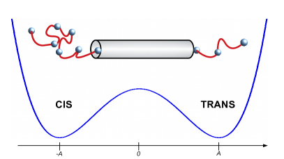
Figure 1: Cartoon of the translocation process of a polymer from CIS to TRANS side of a narrow nanopore. The double-well potential is a caricature of the two-state free energy landscape associated to the translocation.

The nanopore is portrayed as a region of the translocation axis where the polymer feels the effect of an energy barrier, which acts independently on each particle and separates the left-side and right-side of the pore Muthukumar (2010); Ammenti et al. (2009); Polson et al. (2013), see Fig. 1. As customary, in this kind of phenomenology we can assume the evolution of each monomer to be accessible on time-scales long enough to neglect the effect of inertia. Accordingly, the monomers are governed by the overdamped Langevin dynamics:

$$\gamma\dot{x}_{1} = -V^{\prime}(x_{1})+U^{\prime}(x_{2}-x_{1})+\xi_{1}$$

$$\gamma\dot{x}_{i} = -V^{\prime}(x_{i})+U^{\prime}(x_{i+1}-x_{i})-U^{\prime}(x_{i}-x_{i-1})+\xi_{i}$$

$$\gamma\dot{x}_{N} = -V^{\prime}(x_{N})-U^{\prime}(x_{N}-x_{N-1})+\xi_{N}$$ (1)

with $i=2,\ldots,N-1$, where $x_{j}$ is the position of the $j$-th bead. $V$ represents here the external potential, due to the nanopore action on the chain. $U$ is the nearest-neighbor interparticle potential that is chosen to be an even and convex function of $x_{i}-x_{i-1}-\sigma$, where $\sigma$ is the equilibrium distance between consecutive particles. Each $\xi_{i}$ is a Gaussian noise, with average $\langle\xi_{i}(t)\rangle=0$ and correlation $\langle\xi_{i}(0)\xi_{j}(t)\rangle=2\gamma T\delta_{ij}\delta(t)$, where $\gamma$ is a dimensional constant, that we will put equal to 1 in the following.

Let us notice, however, that our interest is not in the behavior of this particular model per se: we are indeed concerned with the general problem of finding proper RCs and their effective evolution equations from data. In this respect, model (1) should be meant as a “generator” of time series. The analysis is not restricted to this specific system, and the same conceptual scheme could be applied to more complex models as well.

As discussed in the Introduction, in order to study the collective dynamics of the polymer we need to identify proper reaction coordinates that describe the state of the system, and then we have to infer effective equations for their evolution.

A natural choice seems to be the center of mass $Q$ of the polymer, which roughly indicates the spatial position of the chain:

$$Q=\frac{1}{N}\sum_{i=1}^{N}x_{i}\,.$$ (2)

Its dynamical equation is obtained by just summing up Eq’s. (1) for all the particles and dividing by $N$,

$$\dot{Q}=-\frac{1}{N}\sum_{i=1}^{N}V^{\prime}(x_{i})+\sqrt{\frac{2T}{N}}\;\eta_{Q}$$ (3)

where the reciprocal elimination of internal forces has been taken into account, as well as the mutual independence of the noises $\{\xi_{i}\}$ that combine into a delta-correlated Gaussian noise with zero mean and such that $\langle\eta_{Q}(0)\eta_{Q}(t)\rangle=\delta(t)$.

By posing $x_{i}=Q+u_{i}$, Eq. (3) can be recast as

$$\dot{Q}=-\dfrac{1}{N}\sum_{i}V^{\prime}(Q+u_{i})+\sqrt{\dfrac{2T}{N}}\;\eta_{Q}\,.$$ (4)

The above equation is formally exact, but it is not very useful in this form, since it depends on all the $u_{i}$ terms.

The roughest approximation that can be done to achieve a closed form for Eq. (4) is to assume that the force term due to the external potential can be written as a (possibly complicated) function of $Q$ only. If this is the case, a one-variable, memoryless model of the kind

$$\dfrac{dQ}{dt}=F(Q)+\sqrt{2D}\,\eta_{Q}\,,$$ (M1)

should catch the relevant features of the macroscopic evolution of the system, where $D=T/N$. Assuming that the above approximation holds, the specific form of $F(Q)$ can be inferred from data, as will be discussed in the following.

Let us notice that Eq. (M1) describes a Markovian stochastic process for the variable $Q$, and it is expected to give a reasonable approximation of the real dynamics only when the knowledge of $Q$ suffices to determine the macroscopic state of the system. For instance, Eq. (M1) gives a good approximation of the real dynamics in the limit of high-rigidity chain, as it will discussed in the following for a particular case.

In general, however, the above one-variable model will not be valid, meaning that it will not be possible to find any form of $F(Q)$ able to reproduce the dynamical properties of the original system in an accurate way. This is due to the fact that the dynamics of $Q$, in general, is not Markovian: in order to achieve a satisfactory coarse-grained description, one possibility is to modify Eq. (M1) by introducing memory-dependent terms, which in some cases can be found analytically by mean of projection methods Zwanzig (1961, 1973); Grabert et al. (1980). To avoid such dependence on memory kernels, which are often difficult to manipulate, the only possibility is to search for (at least) a second RC of the system, such that the vector composed by $Q$ and this new variable obeys a Markovian dynamics.

The additional RC can be individuated through the methods briefly mentioned in the Introduction, or it can be suggested by physical intuition. For instance, one can study a simplified version of the considered problem in order to understand what are the relevant variables. In our case, if the bond fluctuations are large enough, it is reasonable that the elongation $L=x_{N}-x_{1}$ have a role in the macroscopic dynamics. In Appendix A we discuss our system under a strong approximation, which allows a simple analytical treatment: in this context the role of $L$ is transparent. We can then guess an effective model of the form:

$$\begin{cases}\dfrac{dQ}{dt}=F_{Q}(Q,L)+\sqrt{2D_{Q}}\,\eta_{Q}\\ \\ \dfrac{dL}{dt}=F_{L}(Q,L)+\sqrt{2D_{L}}\,\eta_{L}\,.\end{cases}$$ (M2)

Again, assuming that the dynamics of $(Q,L)$ is fairly described by a Markov process, the best choices for $F_{Q}$, $F_{L}$, $D_{Q}$, $D_{L}$ can be found with data-driven approaches as the one used in this paper. However, one has then to verify that the chosen RCs are actually “valid” macroscopic variables, i.e. that the coarse-grained dynamics (M2) reproduces the macroscopic features of the original system.

In the remaining part of this paper, we will try to implement this program in a specific case. In particular we will show that, as expected, the stiffness of the polymer plays an important role in the choice of the right set of RCs.

III Polymer in a double well

We consider now the case in which the external potential $V(x)$ in Eq. (1) is a double-well. This simple model allows us to study some properties of thermally activated barrier crossing as, for instance, the dependence of the jump rate $r$ on the physical parameters.

The general problem of activated dynamics has been extensively studied since the seminal works by Kramers, and the reaction-rate theory provides many analytic methods to compute jump times in different contexts (see Ref. Hänggi et al. (1990) and reference therein). Important results have been derived also for polymeric chains Jun Park and Sung (1999); Sebastian and Paul (2000); Sebastian and Debnath (2006). We want to stress that our aim here is not to improve such results: we are interested in analyzing the ability of a data-driven approach to reconstruct an activated dynamics. In particular, we will focus on the role of the chain stiffness on the activated dynamics and, more importantly, on its relevance for the description in terms of the RCs.

The external potential reads, in this case,

$$V(x)=\frac{B^{2}}{4}(x^{2}-A^{2})^{2}$$ (5)

where $A$ and $B$ are suitable constants. The typical dynamics of the center of mass, $Q(t)$, is therefore characterized by jumps over the barrier separating the two minima of the potential (two-state model). For the interaction potential we choose the form $U(r)=K(r-\sigma)^{2}/2$.

In the following, we will always consider the limit $N\sigma\simeq A$, i.e. the case in which the equilibrium length of the polymer is comparable to the half distance between the well minima: it is reasonable to expect that in these conditions the value of the bond rigidity affects the qualitative behavior of the chain in a relevant way.

Our aim is to show that for high values of $K$ the model described by Eq. (M1) suffices to reproduce the quantitative macroscopic behaviour of the system; whereas, as soon as $K$ becomes comparable to $B^{2}A^{2}/\sigma$, the evolution of $Q$ is no more Markovian and any attempt to describe it through model (M1) is doomed to fail. However, if the phase-space is expanded by including a suitable additional RC, it is still possible that the evolution of the new RCs vector turns out to be Markovian, so that a dynamical description based on Eq. (M2) can be accurate enough.

The validity of such scenario can be tested by using the data-driven approach mentioned in the Introduction and detailed in Appendix B. We first perform numerical simulations of the whole system by using a Stochastic Runge-Kutta algorithm Honeycutt (1992) and measuring the relevant RCs of the system at every time step. As a first attempt, from long time-series of such data we build an effective stochastic equation for $Q$ only, in the form of Eq. (M1); then we apply the extrapolation procedure to the dynamics of the two-dimensional vector $(Q,L)$, obtaining an M2-like model. The “goodness” of M1 and M2 is tested by measuring the Kramers’ transition times of the reconstructed models and comparing the corresponding jump rates to the original ones.

III.1 1-variable model

Before applying the mentioned extrapolation method to infer numerically the functional form of the terms appearing in Eq. (M1), let us derive analytically an effective equation for $Q$ for the high-stiffness limit, $K\gg B^{2}A^{2}/\sigma$. In this case we can assume that the position of two consecutive beads is fixed and equal to $\sigma$. Due to the simple form of the external potential $V(x)$, the drift term in Eq. (4) can be exactly computed in this case:

$$-\frac{1}{N}\sum_{i=1}^{N}V^{\prime}(Q+u_{i}) =-\frac{B^{2}}{N}\sum_{i=1}^{N}\left[(Q+u_{i})^{3}-A^{2}(Q+u_{i})\right]$$ (6)

$$=-\frac{B^{2}}{N}\sum_{i=1}^{N}\left[3Qu_{i}^{2}+Q^{3}-A^{2}Q\right]\,.$$

where we have used the fact that, due to the rigidity of the polymer, $\sum_{i}u_{i}^{3}=\sum_{i}u_{i}=0$.

Now we substitute the explicit expression for the relative positions of the polymer beads, $u_{i}=(2i-N-1)\sigma/2$, and after straightforward algebra we get

$$-\frac{1}{N}\sum_{i=1}^{N}V^{\prime}(x_{i}) =-B^{2}Q\left(Q^{2}-A^{2}+\frac{\sigma^{2}}{4}(N+1)(N-1)\right)$$ (7)

$$=-B^{2}Q\left(Q^{2}-A_{\text{eff}}^{2}\right)$$

with

$$A_{\text{eff}}=A\sqrt{1-\frac{L^{2}(N+1)}{4A^{2}(N-1)}}\,,$$ (8)

where we have used the definition of the polymer length for the rigid case, $L=(N-1)\sigma$. Let us notice that the above drift corresponds to an effective potential

$$V_{\text{eff}}(Q)=\frac{B^{2}}{4}(Q^{2}-A_{\text{eff}}^{2})^{2}\,,$$ (9)

i.e. a “rescaled” version of the original external potential (5).
We can now use the theory of escape times Gardiner (2009) to estimate the jump rate $r$ for the effective potential (9). The average waiting time between two consecutive jumps can be computed through the formula Gardiner (2009)

$$\tau= \frac{1}{D}\int_{-A}^{A}dy\,e^{V(y)/D}\int_{-\infty}^{y}dz\,e^{-V(z)/D}$$ (10)

$$= \frac{1}{D}\int_{-A}^{A}dy\,e^{\frac{B^{2}}{4D}\left[y^{4}-2A_{\text{eff}}^{2}y^{2}\right]}\int_{-\infty}^{y}dz\,e^{-\frac{B^{2}}{4D}\left[z^{4}-2A_{\text{eff}}^{2}z^{2}\right]}$$

where $D=T/N$ is the diffusivity associated to $Q$. The jump rate $r$ is then found as

$$r=\frac{1}{\tau}\,.$$ (11)

The above equations, which are only valid in the rigid-rod limit, will be a useful touchstone to evaluate the level of accuracy of the model inferred numerically.

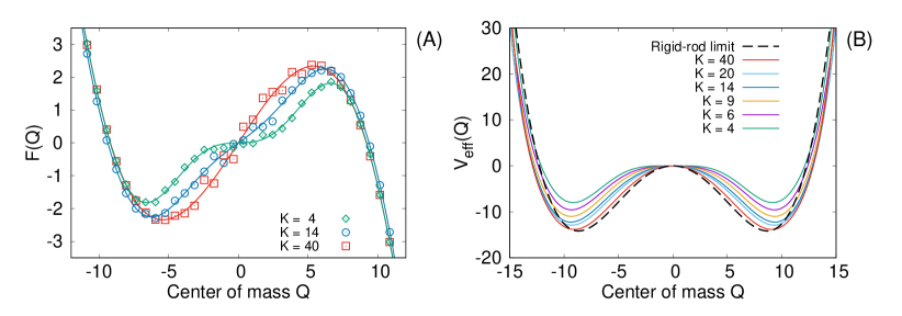
Figure 2: (A): drift term $F(Q)$ of model (M1) as reconstructed from data (points) and fitted with a 9-th degree odd polynomial (solid lines), for three different values of $K$. (B): Effective potential obtained by integration of $F(Q)$. Parameters for the simulations of the complete system: $A=10$, $B=0.1$, $T=30$, $\sigma=1$, $N=10$, using a time-step $dt=10^{-5}$. Simulations on model (M1) have been run with a time-step $dt=10^{-4}$.

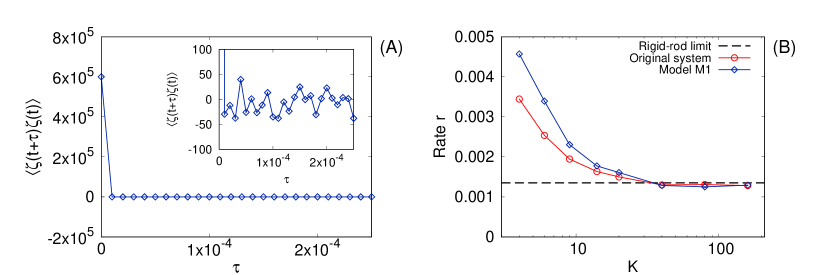
Figure 3: Checking the validity of model (M1). (A) Autocorrelation $\langle\zeta(t)\zeta(t+\tau)\rangle$ of the “noise” term (12) vs. $\tau$. The inset is a zoom. It is apparent the fast decay with $\tau$ that can be considered effectively a delta-correlation, since the time-step of the integration algorithm generating the dynamics is $dt=10^{-5}$. Here, $K=14$. (B): Jump rates as functions of $K$ in the original system (red circles) and in simulations of the reconstructed M1 (blue diamonds). The rigid-rod approximation (dashed line) is reported as reference. Parameters as in Fig. 2.

We apply now the extrapolation procedure mentioned in the Introduction and detailed in Appendix B to infer the right functional forms for the terms of the Langevin equation (M1), assuming that the dynamics of $Q$ is Markovian and a 1-variable description in the form of model (M1) holds. We find that $D$ (not shown here) is always almost constant and equal to $T/N$, as it would be expected if the process was Markovian, while the drift shows a more complex shape (Fig. 2A); we fit the data by a 9-th degree, odd polynomial, then we integrate the resulting function in order to get an effective potential, which is reported in Fig. 2B for several values of $K$. In the large-$K$ limit, as expected, we recover a quartic effective potential: terms of higher order become relevant when the bond stiffness is low, and their effect is to flatten the potential barrier between the two wells.

As mentioned above, the validity of Eq. (M1) relies on the assumption that the evolution of $Q$ is Markovian, which has to be checked. First, one can define and measure the following quantity:

$$\zeta(t)=\dot{Q}(t)-F(Q(t))\,,$$ (12)

which represents the “noise” of Eq. (M1), if the dynamics of $Q$ is Markovian. We can compare the autocorrelation time of $\zeta(t)$ and verify that it is much shorter than any characteristic time-scale of the dynamics of $Q$. In our case, $\zeta(t)$ always decorrelates on the scale of the time-step of the integration algorithm, $dt$ (see Fig. 3A).

This first check assures that there is a clear time-scale separation between the dynamics of the center of mass and its “noise”. However, this does not imply that the original dynamics of $Q$ has to be Markovian: in order to check that, we also have to verify the consistency with the original dynamics. If the one-variable description is able to catch the relevant features of the whole system, we can conclude, a posteriori, that the evolution of $Q$ was Markovian also in the complete dynamics; if not, a different description has to be taken into account.

Fig. 3B shows, for several values of the rigidity, the jump rates measured in the original dynamics and those observed in the reconstructed model, using a standard stochastic integration algorithm (the one discussed in Mannella and Palleschi (1989), up to order $dt^{3/2}$). In the high-$K$ limit the simple rigid-rod approximation (10) holds, there is no dependence on $K$ and the agreement between the jump rates of M1 and of system (1) is excellent. As the polymer becomes softer, even if a significant improvement on Eq. (10) can be observed, the relative error between M1 and the true dynamics exceeds 30%: this is a clear hint that a 1-variable description, even if inferred directly from data, cannot reproduce all the relevant features of the dynamics. This is due to the fact that our implicit assumption on the Markovianity of the process is wrong.

III.2 2-variables model

The failure of model (M1) for small values of $K$, revealed by the discrepancies between the reconstructed and the original jump rate, suggests to go beyond a single variable description in order to achieve satisfactory results. As discussed in Section II, a reasonable attempt to recover a Markovian dynamics is to consider the elongation of the polymer, $L$, as a second $RC$ for our model, and we postulate the validity of an evolution equation of the form (M2).

The requirement of a variable accounting for the elongation of the polymer can be easily understood by looking at Fig. 4 reporting three scatter plots of the original dynamics in the $(Q,L)$ plane, for different bond rigidity, where $L=x_{N}-x_{1}$. When $K$ is high, and the system is well approximated by the rigid-rod model, the region of the phase space explored by the dynamics is a thin strip around the equilibrium value $L\simeq(N-1)\sigma$. As soon as the rigidity condition is relaxed, and the system is allowed to vary its length in a significant way, a two-lobe distribution takes place: $L$ tends to be smaller than the rest length of the chain when the polymer occupies one of the two minima of the double-well potential, while it significantly increases during the transition across the barrier. This particular shape of the scatter plot indicates that the typical pathways in the space $(Q,L)$ include a non-negligible deformation in $L$, which can be straightforwardly interpreted as follows: when the rigidity $K$ is low, the transition across the barriers of the polymer occurs with a concomitant stretching of the bonds, presumably those that instantaneously lay on top the barrier. As a consequence, any Markovian effective description involving only the center of mass is completely insufficient to fairly approximate the dynamics of the system.

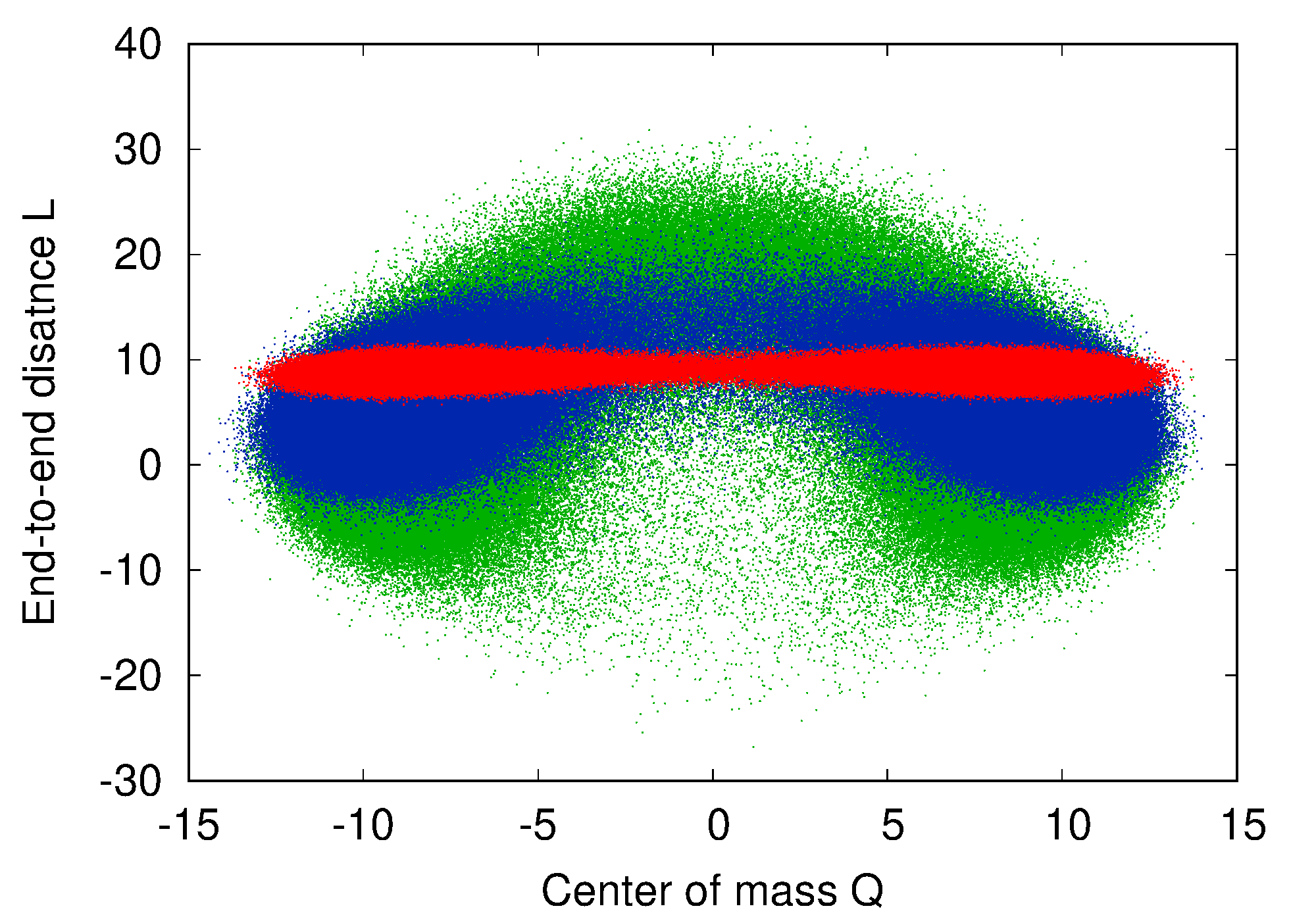
Figure 4: Scatter plot of the end-to-end distance $L$ vs. $Q$ (total integration time: $10^{6}$). Green dots: $K=4$; blue dots: $K=20$; red dots: $K=600$. Other parameters as in Fig. 2.

Following again the strategy discussed in Appendix B, we provide numerical values for $F_{Q}$, $D_{Q}$, $F_{L}$ and $D_{L}$ in the $(Q,L)$ space, which have to be fitted using suitable functional forms. Due to the symmetries of the system, $F_{Q}(Q,L)$ has to be odd with respect to the variable $Q$, while $F_{L}(Q,L)$ should be even. Fig. 5 shows the results obtained by fitting the following polynomial form:

$$F_{Q}(Q,L) =Q\left[c_{10}^{(Q)}+c_{12}^{(Q)}L^{2}+c_{13}^{(Q)}L^{3}\right]$$ (13)

$$+Q^{3}\left[c_{30}^{(Q)}+c_{32}^{(Q)}L^{2}+c_{33}^{(Q)}L^{3}\right]$$

$$F_{L}(Q,L) =c_{00}^{(L)}+c_{01}^{(L)}L+c_{03}^{(L)}L^{3}+c_{21}^{(L)}Q^{2}L\,.$$

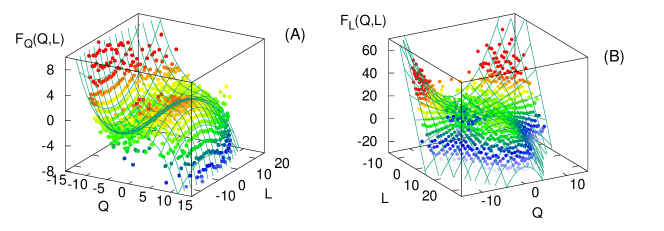
Figure 5: Reconstructed drift terms of $Q$ and $L$ in the model (M2), case $K=4$. Points are extrapolated from data (see Appendix B); the surface is obtained by fitting the polynomial (13). Other parameters are as in Fig. 2.

The agreement between the actual data and the proposed functional form is good enough to hope that the guessed model catches the most relevant features of the dynamics. The diffusivity terms $D_{Q}$ and $D_{L}$ are again fitted by constant functions. Once model (M2) is determined, we can check the reliability of its stochastic evolution by a direct comparison with the original dynamics.

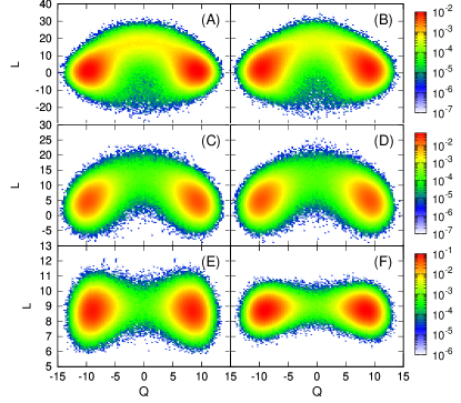
Figure 6: Pdfs in the 2-variable phase space of the original system, first column, and in the reconstructed 2-variables model (M2), second column. Stiffness: $K=4$ (top), $K=20$ (center), $K=600$ (bottom). Other parameters are the same as Fig. 2.

A first, important benchmark is given by the ability of the model to reproduce the static properties of the system, namely the joint probability distribution in the $(Q,L)$ space. This test is reported in Fig. 6 for different values of $K$, showing a reasonable qualitative agreement even in the non-trivial case of low bond stiffness: in particular, the stretching occurring when the polymer crosses the barrier is clearly reproduced.

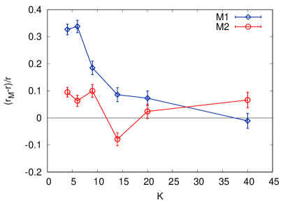
Figure 7: Relative errors of the jump rates $r$ in the two reconstructed models, varying $K$. For other parameters, see caption of Fig. 2.

The improvement of our effective description when also $L$ is taken into account can be fully appreciated by looking at dynamical observables as the jump rate $r$. Fig. 7 displays the relative errors between the values of $r$ obtained in the reconstructed models M1, M2 and in the original dynamics. As already discussed, the 1-variable model fails when the polymer is soft, while the accuracy of M2 does not seem to be affected in this limit. Let us notice, on the other hand, that for $K\gg A^{2}B^{2}/\sigma$ the reconstructed model (M2) is less reliable than the 1-variable version: this is probably a consequence of the larger number of parameters involved, which leads to a lower degree of precision on their determination with the discussed method.

III.3 Remarks on the structure of the effective equations

The procedure for the reconstruction of a model in the form (M2) that we used in the previous subsection is based on a “dynamical” analysis, which builds the coefficients of the guessed stochastic model by looking at the time evolution of suitable observables of the original system (see Appendix B). One could wonder whether such procedure is really needed in order to get a realistic description of the studied process; for example, in analogy with many statistical mechanical problems, one may expect that the following recipe works:

1. measure the stationary p.d.f. $\rho(Q,L)$ from long time series of data;

2. deduce an effective 2-variable “potential”, also known as “potential of mean force” in chemical and biophysical contexts:

   $$W_{S}(Q,L)=-\log[\rho(Q,L)]\,;$$ (14)

3. define $F_{Q}\equiv-c\partial_{Q}W_{S}$ and $F_{L}\equiv-c\partial_{L}W_{S}$, where the constant $c$ has to be determined.

Let us notice that in many practical situations the multidimensional free-energy landscapes obtained by simulations or experiments are assumed to be generated by a system with a gradient (or gradient-like) structure and, using this hypothesis, Langer’s formula Langer (1969); Hänggi et al. (1990) is applied to derive the transition rates over saddles.

The above procedure is a completely “static” analysis, because it involves only quantities measured in equilibrium conditions. Leaving apart the problem of finding the right multiplicative constant $c$ and the noise terms, this approach has a major issue: it is not sure, a priori, whether the dynamics of the chosen reaction coordinates can be described by a potential, even if the complete system actually can; in other words, there is in general no reason to expect that the model is a gradient system in the reduced phase space.

The knowledge of $W_{S}$ alone is not sufficient to obtain the drift; additional informations on the dynamics need to be taken into account. A possibility is the theoretical approach discussed in Ref. Grabert (2006), which also involves the transport coefficients. Our numerical method, instead, exploits the dynamical information by computing suitable conditioned moments of the RCs, as discussed in Appendix B.

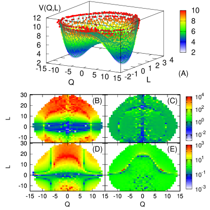
Figure 8: Static analysis. (A): effective potential $W_{S}(Q,L)$ from the empirical pdf in the $(Q,L)$ space. Panels below compare the drift computed with this static approach, $\nabla W_{s}$, and the one reconstructed with our dynamical approach, $(F^{(2)}_{Q},F^{(2)}_{L})$, to the measured coefficients $F_{Q},F_{L}$. (B): $|\partial_{Q}W_{s}/F_{Q}|$. (C): $|F^{(2)}_{Q}/F_{Q}|$. (D): $|\partial_{L}W_{s}/F_{L}|$. (E): $|F^{(2)}_{L}/F_{L}|$.

In order to show that in our case the simplifying assumption of a gradient structure for the $(Q,L)$ dynamics is wrong, let us determine $W_{S}$ using Eq. (14). In Fig. 8A we fit such “potential” with a 2-variable polynomial (4-th order in both $Q$ and $L$), getting a nice superposition.

If the 2-variables system were gradient, $F_{Q}(Q,L)$ should be equal to $c\partial_{Q}W_{S}$, for some value of $c$; therefore the ratio $\partial_{Q}W_{S}/F_{Q}$ should be constant all over the phase-space. Fig. 8B shows instead that, in our case, such function strongly depends on $Q$ and $L$. Just for comparison, Fig. 8C displays the ratio

$$\epsilon=F^{(2)}_{Q}/F_{Q}$$

where $F^{(2)}_{Q}$ represents here the expression from the fitting (13): not surprisingly, this function is constant and equal to one almost everywhere, meaning only that we have made sensible choices for the polynomial functions to use in the fit. In Fig. 8D, 8E the same comparison is done for the drift of the end-to-end distance $L$.

This simple check clearly shows that the simplified 2-variables system is not gradient, and therefore a static analysis is not sufficient to infer reasonable effective equations for its evolution.

IV Conclusions

We studied the dynamics of a 1-dim polymer whose monomers are subjected to a double-well external potential. Under certain conditions, the phenomenology is characterized by thermally activated barrier crossing (classical Kramers’ problem). We addressed the issue of describing this complex high-dimensional dynamics in terms of few suitable observables, the reaction coordinates (RCs). In our system the center of mass, $Q$, and the end-to-end distance, $L$, are the most natural candidates.

These RCs evolve according to effective Langevin equations that are generally difficult to be derived via a systematic procedure. The proper reconstruction of the effective stochastic equations for $Q$ and $L$ is achieved via a data-driven numerical method that extrapolates the drift and diffusion terms from a long trajectory of the original system. Let us stress that this method allows us to find nonlinear terms for the reconstructed Langevin equation; this is an important difference, e.g., from the standard Mori-Zwanzig approach, where the complexity of the problem is shifted into the shape of the memory kernels. Zwanzig (1961) The reliability of the reconstructed dynamics is tested on the way it fairly reproduces some essential properties of the original dynamics, such as a correct estimate of the jump rate over the barrier.

From our study it emerges that the description level in terms of RCs strongly depends on the bond stiffness $K$. More precisely: if the bonds are rigid enough, we are allowed to consider the evolution of $Q$ only, given by model (M1), to fully characterize the jump dynamics. However, when $K$ decreases, the internal motion of the chain cannot be neglected and also the dynamics of $L$ has to be considered, so that a satisfactory description can only be obtained in the plane $(Q,L)$ through the model (M2). On a more mathematical perspective, lowering $K$ can be regarded as a loss of Markovianity of the one-variable description. A second coordinate is necessary to recover the Markov property.

Our work shows how subtle is the procedure of reducing the dynamics of a many-dimensional system to a low-dimensional model, even in the simplest cases where the physical intuition leaves little ambiguity to the choice of the RCs. In fact, the choice of an RC can be correct in certain regimes but not sufficient in others. Specifically in our case, we can only know a posteriori that it is the stiffness of the polymer to determine whether one or two RCs are needed.

Appendix A The homogeneous chain approximation

In this Appendix we discuss the “homogeneous chain approximation” (HCA), which amounts to assuming that the distances between nearest-neighbor particles, at each time $t$, are all equal:

$$x_{i+1}(t)-x_{i}(t)=x_{j+1}(t)-x_{j}(t)\,,\quad\forall i,j\,.$$ (15)

Under such approximation we can derive closed analytical expressions for both models (M1) and (M2); HCA is very unphysical, and it only holds true if the polymer bonds are almost rigid. However, a simple analysis of this limit can give us some insight on the general case. Even under such simplifying hypotheses, as soon as $K$ is large enough, model (M1) is not sufficient to describe correctly the dynamics, and a (M2)-type model is needed.

First, let us consider the case of high intra-chain forces acting on each monomer. Specifically, the bonds are much stronger than: i) the external forces due to the action of the potential $V(x)$ and ii) those induced by the thermal fluctuations. Under conditions i) and ii) our polymer reduces to a rigid rod with fixed distances among its elements, i.e.

$$x_{i+1}(t)-x_{i}(t)=const\quad\forall i\,.$$ (16)

Eq. (4) can be written as

$$\dot{Q}=-\int\!\!du\rho(u)V^{\prime}(Q+u)+\sqrt{\dfrac{2T}{N}}\;\eta_{Q}\;.$$ (17)

where we have introduced the density, $\rho(u)=1/N\sum_{i=1}^{N}\delta(u-u_{i})$, to pass from the sum to an integral. Here

$$\rho(u)\simeq\frac{1}{L}\Theta(u^{2}-L^{2}/4)\,,$$ (18)

where we also took the $N\gg 1$ limit. The total length of the polymer is constant, $L=(N-1)\sigma$.

In this simple case, we can straightforwardly apply the fundamental theorem of calculus and get:

$$\dot{Q}=\dfrac{1}{L}[V(Q-L/2)-V(Q+L/2)]+\sqrt{\frac{2T}{N}}\eta_{Q}\,.$$ (19)

Notice that the above equation is of the form of model (M1).

Let us consider now the idealized situation in which the inter-particle distances do fluctuate, but the approximation (19) still holds because the polymer undergoes homogeneous deformations. In this limit, the end-to-end distance $L$ defined as

$$L=x_{N}-x_{1}$$ (20)

is no longer constant and Eq.(19) should be complemented by a new equation describing the dynamics of $L$. Now $L$ is a necessary second RC, so the phase space is enlarged to the plane $(Q,L)$.

Under this hypothesis, we can derive a second equation, by writing $\dot{L}=\dot{x}_{N}-\dot{x}_{1}$ from Eq. (1) and then approximating each $x_{i}-x_{i-1}\simeq L/(N-1)$. The final result for the drift expressions is

$$F_{Q}(Q,L) = \dfrac{1}{L}\left[V\left(Q-\dfrac{L}{2}\right)-V\left(Q+\dfrac{L}{2}\right)\right]$$

$$F_{L}(Q,L) = -2U^{\prime}\left(\frac{L}{N-1}\right)+V^{\prime}\left(Q-\frac{L}{2}\right)-V^{\prime}\left(Q+\frac{L}{2}\right)$$

The above phenomenological discussions suggest that there are two regimes depending on the polymer stiffness:

• stiff chain: the polymer dynamics can be characterized by a single reaction coordinate $Q$, for which a closed evolution equation can be found;

• soft chain: also a second variable, for instance the end-to-end distance $L$, is needed to close the evolution equations.

Notice that in the above discussion the introduction of $L$ as a second $RC$ emerges quite naturally. This can be a clue on the relevant variable to choose also in the more general case where assumption (15) does not hold.

Appendix B Extrapolating Langevin equations from data

In this Appendix we briefly recall the basic aspects of the extrapolation procedure that we use to infer the parameters of effective Langevin equations from long-time series of data (in this case, produced by numerical simulations). An extensive discussion of the method can be found in Kleinhans et al. (2005); Baldovin et al. (2018a) and reference therein. See also Baldovin et al. (2019) for a case in which the study of a multi-dimensional system is considered.

Let us assume that each component of the vector variable $\mathbf{X}$ obeys the following Langevin’s equation:

$$\dot{X}_{i}=F_{i}(\mathbf{X})+\sqrt{2D_{i}(\mathbf{X})}\xi_{i}\,$$ (22)

where each $\xi_{i}$ is a white noise with unitary variance. For the sake of simplicity, here we assume that the coefficients $F_{i}$ and $D_{i}$ do not depend on time. It can be proved Friedrich et al. (2011) that the following relations hold:

$$F_{i}(\mathbf{x}) =\lim_{\Delta t\to 0}\frac{1}{\Delta t}\langle\Delta X_{i}|\mathbf{X}(0)=\mathbf{x}\rangle$$ (23)

$$D_{i}(\mathbf{x}) =\lim_{\Delta t\to 0}\frac{1}{2\Delta t}\langle\left(\Delta X_{i}-F_{i}(\mathbf{x})\Delta t\right)^{2}|\mathbf{X}(0)=\mathbf{x}\rangle$$

where $\Delta X_{i}=X_{i}(\Delta t)-X_{i}(0)$. Due to the stationarity of the process, we can compute the ensemble averages (23) as temporal averages over long-time series of data.

The $\Delta t\to 0$ limit has to be interpreted in a proper physical way: for every real phenomenon, a stochastic description holds only for some not-too-small time scales. It is customary to define a typical time-scale of the considered problem, usually referred to as the “Markov-Einstein time” $\tau_{ME}$, such that the Langevin equations hold true only if one considers time scales larger than $\tau_{ME}$. In order to get a reasonable esteem of the above limits, a good strategy is that of plotting the conditioned moments on the r.h.s. of Eq. (23) as functions of $\Delta t$, then to individuate a sufficiently regular region that allows for a $\Delta t\to 0$ extrapolation. In our case, however, the separation of time-scales is a consequence of the fast decorrelation times of the quantity $\zeta(t)$ defined by Eq. (12), which is in turn due to the overdamped nature of the original dynamics we are considering. As a consequence, it is sufficient to take $\Delta t\gg dt$, where $dt$ is the time-step of the integration algorithm. Let us notice once again that such time-scale separation does not imply the Markovianity of the considered process, and the validity of such approximation can be only checked a posteriori.

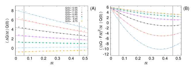
Figure 9: Extrapolation of the drift (panel A) and diffusivity (panel B) from data. The quantities in the rhs of Eq. (23) are fitted with a low-order polynomial; only the regions within the vertical bars are considered for the fit. The $\Delta t\to 0$ limit is then taken as the vertical intercept of the fitted functions with the $y$-axis. Here $K=4$ (other parameters as in Fig. 2).

In Fig. 9 we show a typical case of reconstruction of the drift and diffusivity terms of model (M1), for several values of the center of mass.