KISS: Keeping It Simple for Scene Text Recognition

Abstract

Over the past few years, several new methods for scene text recognition have been proposed. Most of these methods propose novel building blocks for neural networks. These novel building blocks are specially tailored for the task of scene text recognition and can thus hardly be used in any other tasks. In this paper, we introduce a new model for scene text recognition that only consists of off-the-shelf building blocks for neural networks. Our model (KISS) consists of two ResNet based feature extractors, a spatial transformer, and a transformer. We train our model only on publicly available, synthetic training data and evaluate it on a range of scene text recognition benchmarks, where we reach state-of-the-art or competitive performance, although our model does not use methods like 2D-attention, or image rectification. Code and model are available on Github .

1 Introduction

Text is a ubiquitous entity that provides high level semantic information. Text can not only be found in written documents such as letters or bills, but also in natural scenes on, e.g., road signs, billboards, store fronts, etc. Being able to localize and recognize text in a natural scene image is very useful for a range of applications, such as navigation systems, content-based image retrieval, image-based machine translation, or even as support for visually impaired people. Developing more accurate and robust recognition systems for scene text has been a widely researched challenge for several years [11, 13, 19, 24, 28, 30]. Accurate and robust localization and recognition of scene text is a challenging problem, because text in natural scenes appears in various forms, can be heavily distorted, blurred, or placed on challenging backgrounds.

With the emergence of deep learning methods, the performance of scene text localization and recognition systems has been boosted significantly. Especially advances in the fields of synthetic data generation [11], attention modeling [1], or semantic segmentation [6] pushed the state-of-the-art significantly. In this paper, we focus on scene text recognition, which is the task of recognizing the textual content of an image that contains a single cropped word. In recent time, a lot of sophisticated solutions for this task have been developed. Such sophisticated solutions include, but are not limited to: neural networks that learn to rectify an input image [29, 41], neural networks that incorporate attention mechanisms tailored specifically for the task of scene text recognition [21, 29], or methods that formulate the problem as a semantic segmentation task [19]. For more information on related work and how other work relates to our work, please see Section 2.

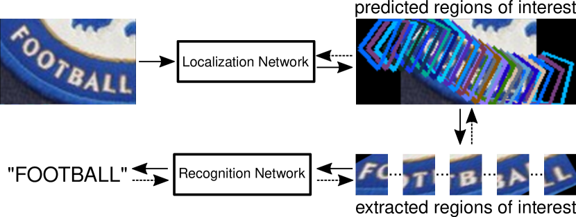
Figure 1: Our proposed system consists of two independent neural networks that are jointly trained. The localization network predicts regions of interest that belong to the characters of the word in the image. We then use a spatial transformer to extract the regions from the image. The extracted regions are then fed into the recognition network that uses all extracted regions of interest to predict the textual content of the image. The model is end-to-end trainable (indicated by dotted lines) using only word-level annotations.

In this paper, we propose a novel scene text recognition network that does not use any building blocks especially designed for the task of scene text recognition. We rather use off-the-shelf components for building a neural network architecture, do not use any tricks like fine-tuning to train our network, or any non-public datasets, while still being able to reach competitive/state-of-the-art accuracy on a range of several scene text recognition benchmarks. Our proposed model KISS (the name is based on the KISS principle [25], which says that a simple solution should be preferred over a more complex one) is straight forward and simple. It consists of two ResNet-18 feature extractors [7], a spatial transformer [12] and a transformer [36] (see Figure 1 for a high-level overview of our system). Our two networks work together as a team. The first network identifies regions of interest in the cropped word image. Those regions of interest are predicted as affine transformation matrices that are used by the spatial transformer to crop those regions from the input image and provide them as input to the second network. The second network now extracts features from each region of interest and uses a transformer to predict the character sequence contained in the image. We train our model from scratch and use only publicly available synthetic datasets for training our model. Further information on the design of our neural network can be found in Section 3.

We evaluate the proposed model on a variety of standard scene text recognition benchmarks and show that our model reaches competitive/state-of-the-art performance on all benchmarks. We also conduct an ablation study, providing further insight into the importance of individual building blocks of our model. More information on our experiments can be found in Section 4.

The contributions of this paper can be summarized as follows: (1) we propose a novel network architecture that builds on the cooperation of two independent neural networks, where one network learns by itself how to support the second network. (2) The proposed model architecture is based on off-the-shelf neural network components, like ResNets, a spatial transformer and a transformer. (3) Our model reaches competitive/state-of-the-art recognition accuracy on a range of benchmark datasets for scene text recognition. (4) We show which building blocks are the most important for a state-of-the-art scene text recognition system.

2 Related Work

Over the course of time a wide variety of different methods for scene text recognition has been proposed. Especially with the upcoming of methods based on deep learning, the performance of systems in the domain of scene text recognition was boosted significantly. While the first methods used binarization methods and standard print ocr systems [24], or sliding window methods with random ferns [37] for the task of scene text recognition, more recent methods are fully based on directly applying learned feature extractors, based on deep neural networks for the task of scene text recognition. Jaderberg et al. propose one of the first deep learning based methods for scene text recognition [13] where they use a deep neural network for character classification that is applied in a sliding window fashion, on a cropped word image. Later, Jaderberg et al. propose to directly apply a deep neural network on a cropped word image and predict each character with an individual softmax classifier [11].

Later approaches incorporate a recurrent neural network after the convolutional feature extractor, in order to utilize the capabilities of recurrent neural networks to capture sequences. Shi et al. propose one of the first scene text recognition models that are based on a convolutional feature extractor and a recurrent neural network [28]. He et al. also propose a model based on a convolutional feature extractor and a recurrent neural network, but they utilize the recurrent neural network on features extracted from crops of the word image, which have been obtained in a sliding window fashion [8], which is different from [28], where they use the complete word image as input to their convolutional feature extractor. Compared to our method, the method by He et al. method only uses a very simple and inflexible sliding window method that neither adapts to the number of characters in the image, nor the orientation of the characters in the image.

The idea of using a recurrent neural network to predict a character sequence has since been extended by various methods that incorporate an attention mechanism into the character sequence prediction [17, 18, 19, 21, 29, 30, 39, 41]. Liu et al. [21] propose a neural network that includes a spatial transformer network [12] which is used to put focus on the features of single characters. They produce their character predictions using a special hierarchical character attention layer and a LSTM, following the spatial transformer and convolutional feature extractor.

The methods [29, 30, 41] first utilize a spatial transformer network that predicts a thin plate spline transformation to rectify the textual content of the input image. Then, they extract features from the rectified image with a convolutional feature extractor, followed by a recurrent neural network, with different forms of attention, for character prediction. In [29, 30] Shi et al. utilize a sequence-to-sequence network that consists of a bidirectional LSTM as encoder and an attention guided GRU as decoder. Zhan & Lu [41] rectify the input image multiple times before using a ResNet [7] based sequence-to-sequence recognition network with attention. The approach introduced by Luo et al. [22] also follows the path of image rectification before recognizing the textual content of the cropped word image, but they do not use spatial transformers to predict the necessary rectification transformation. Instead, they predict an offset map that is applied to each pixel, achieving a differentiable sampling procedure.

Our method does not use any specialized attention methods, instead we use the spatial transformer network to generate regions of interest that (in the ideal case) contain a single and (ideally) rectified character. We then feed the extracted region of interest into our second network that uses a transformer [36] to predict single characters.

In [4] Cheng et al. introduce an approach for the recognition of arbitrarily oriented text. Their approach consists of a network that uses features from 4 different spatial directions, together with a special attention mechanism to predict the textual content of the image. In contrast to our approach, this approach consists of several newly introduced and complicated building blocks that help to boost the recognition performance of the model.

Other approaches directly utilize information about the bounding box of individual characters for the generation of their predictions. Wang et al. [39] propose to use a convolutional LSTM [31] on top of a convolutional feature extractor with a special mask based attention mechanism for the prediction of characters. One approach by Liao et al. formulates the task of scene text recognition as a semantic segmentation task and they create a fully convolutional network that predicts a segmentation encoding the position and class of each character [19]. Both methods need ground-truth bounding boxes for each character, constraining their possible extensibility, as it is expensive to obtain such a full labeling. Our method also localizes individual characters, but without the need for labeled character bounding boxes, making it simpler to apply our method to new datasets. Another approach by Liao et al. [18] utilizes a sequence-to-sequence network with attention guided GRU. They utilize a two dimensional feature map as input to their attention guided decoder, which is similar to the work by Shi et al. [30], but they do not use a rectification network.

Wang et al. [38] also propose a simple network that only consists of a feature extractor and a transformer for scene text recognition. In our work, we also use a transformer, but we train it in a different way.

A method that highly influenced our work, is the work by Bartz et al. [3]. They propose a neural network architecture for the task of end-to-end scene text recognition and show that a model can be trained for text localization and recognition, solely under the supervision of a text recognition based objective. We build on their approach and make fundamental changes to the overall network structure.

3 Method

Our network consists of two parts. We call the first part localization network and the second part recognition network. Our localization network consists of a ResNet based feature extractor and a spatial transformer that produces the input to the second network and allows us to train localization network and recognition network at the same time. The recognition network consists of a ResNet based feature extractor and a transformer. The recognition network takes regions of interest as input and produces a character sequence as output. In Figure 2 we provide a structural overview of the proposed network. In this section we present each building block in detail and also introduce a novel method that is necessary to successfully train the whole network.

3.1 Localization Network

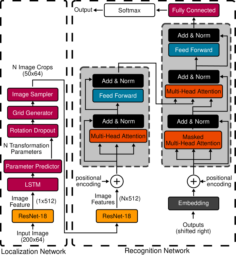
Figure 2: The network architecture proposed in this work consists of two sub-networks. Each network first extracts features using a ResNet-18 feature extractor. The first network then produces $N$ regions of interest, using a recurrent spatial transformer. Each of these $N$ regions is then used as input to the recognition network. The recognition network then uses a transformer to predict the textual content of the input image, after extracting features with the ResNet-18 feature extractor.

The task of the localization network is to predict regions of interest that (ideally) contain a character. The localization network is trained by the recognition network, which in turn is trained using word-level annotations. Our localization network consists of a convolutional feature extractor and a recurrent spatial transformer, as can be seen on the left hand side of Figure 2.

Feature Extractor

We use a convolutional neural network based on the ResNet [7] architecture, as our convolutional feature extractor. We choose to use a ResNet based feature extractor because ResNet does not suffer from the vanishing gradient problem, as much, as other network architectures, such as, VGG [32], or Inception [34] do.

Spatial Transformer

Following the convolutional feature extractor, we use a spatial transformer [12]. The task of the spatial transformer is to extract regions of interest, that are likely to contain a character. In order to extract these regions of interest the spatial transformer consists of three different parts: 1. a transformation predictor, 2. a grid generator, and 3. a differentiable image sampler.

The transformation parameter predictor uses the features that have been extracted by the feature extractor and predicts a series of $N$ affine transformation matrices $A^{n}_{\theta}$. The parameter $N$ is the maximum number of characters our system shall predict. In all of our experiments we follow the setting of Jaderberg et al. [11] and set $N$ to $23$. Those affine transformation matrices can be used to perform affine transformations like scaling, rotating, translating or skewing the pixels of the input image. Each transformation matrix $n$ with $n\in[0,N)$ consists of six parameters $\theta$ that are predicted using the extracted features:

$$A^{n}_{\theta}=\begin{bmatrix}\theta^{n}_{1}&\theta^{n}_{2}&\theta^{n}_{3}\\ \theta^{n}_{4}&\theta^{n}_{5}&\theta^{n}_{6}\end{bmatrix}.$$ (1)

Each of these matrices $A^{n}_{\theta}$ is predicted using a recurrent neural network, in our case a LSTM [9]. At each timestep $n$ of our LSTM we use a fully connected layer with $6$ neurons to predict the transformation matrix $A^{n}_{\theta}$. We use rotation dropout [3], which works like dropout [33] but only drops the parameters $\theta^{n}_{2}$ and $\theta^{n}_{4}$, of the transformation matrix $A^{n}_{\theta}$. These parameters are responsible for performing rotations on the input image. During all of our experiments we set the dropout rate to $0.05$.

The next part of the spatial transformer is the grid generator. The grid generator uses the predicted transformation matrices to create a set of $N$ sampling grids with width $w_{o}$ and height $h_{o}$. Those sampling grids provide the coordinates $u^{n}_{i},v^{n}_{j}$ (with $i\in[0,w_{o})$ and $j\in[0,h_{o})$) that are used to sample from the input image, using the differentiable image sampler. The size of each grid defines the size of the output of the spatial transformer. This allows us to use images of different input sizes in the localization network, while maintaining a fixed input size for the recognition network. The coordinates $u^{n}_{i},v^{n}_{j}$ are produced by multiplying the coordinates $x_{i},y_{j}$ ($x,y=[-1,\ldots,1]$) of an evenly spaced grid $G$ with one of our predicted transformation matrices $A^{n}_{\theta}$:

$$\begin{pmatrix}u^{n}_{i}\\ v^{n}_{j}\end{pmatrix}=\begin{bmatrix}\theta^{n}_{1}&\theta^{n}_{2}&\theta^{n}_{3}\\ \theta^{n}_{4}&\theta^{n}_{5}&\theta^{n}_{6}\end{bmatrix}\begin{pmatrix}x_{i}\\ y_{j}\\ 1\end{pmatrix}.$$ (2)

Previous work [3, 29, 30, 41] proposes to initialize the parameter predictor for the affine transformation matrix $A^{n}_{\theta}$ in such a way that a box spanning a large portion of the image is predicted. They claim this is necessary, because otherwise the network would not converge. We, on the contrary, found that randomly initializing the parameter predictor works very well and even helps to speed up the convergence of the model. However, we found that extra regularization is necessary, for a network with a randomly initialized parameter predictor to converge. Without extra regularization, the network tends to predict transformation parameters that produce regions of interest that are far outside of the bounds of the input image. Since regions out of the bounds of the image only contain zeros, the network can not learn from these examples anymore, keeping the network from converging. In order to encourage the network to not predict such transformation parameters, we propose an out-of-image regularizer that is directly applied on the sampling grid, generated by the grid generator. Since the coordinates $x$ and $y$ of the grid $G$ are in the interval $[-1,\ldots,1]$, thus spanning the entire image before the application of our predicted transformation matrix, we know that each value for $u$ and $v$ should exactly be within this interval, in order to be inside of the image. We can now create a regularizer that penalizes each predicted value $u$ and $v$ if they are not in the interval:

$$reg(c)=\lvert min(c+1,0)\rvert+max(c-1,0).$$ (3)

With $c$ being any value from $u$ and $v$. The value of $reg(u)$ and $reg(v)$ can be added to the overall loss of the network, as shown in Equation 8.

The last part of the spatial transformer is the image sampler [12]. The image sampler uses the predicted sampling grids to crop the corresponding pixels from the input image in a differentiable way. Since the sampling points of the predicted sampling grid do not perfectly align with the discrete grid of pixels in the input image, bilinear sampling is used. The image sampler produces $N$ different output images $O^{n}$, where each output image has the same size, as the sampling grid, used for sampling the pixels. Each pixel of the output image $O^{n}$ is then defined to be:

$$O^{n}_{ij}=\sum^{H}_{h}\sum^{W}_{w}I_{hw}max(0,1-\lvert u^{n}_{i}-h\rvert)max(0,1-\lvert v^{n}_{j}-w\rvert).$$ (4)

Where $I$ is the input image with width $W$ and height $H$.

3.2 Recognition Network

The recognition network is the most important part of our proposed system. The recognition network takes the regions of interest that have been extracted by the localization network, or any other method, and predicts the character sequence contained in these region images. The right hand side of Figure 2 provides a schematic overview of the recognition network. This network is trained using word-level annotations and can propagate its gradients to an upstream network, in our case the localization network. The recognition network consists of a convolutional feature extractor and a transformer that predicts the sequence of characters in the image. The convolutional feature extractor is, as the feature extractor of the localization network, based on the ResNet-18 architecture.

Each region of interest that is used as input to the recognition network is processed independently by the feature extractor. The extracted features are used as input to the transformer and a sequence with $N$ elements is formed, based on the output of the localization network. For our transformer, we follow the design introduced in [36]. A transformer consists of an encoder and a decoder. The encoder takes the extracted features of our $N$ regions of interest, adds a positional encoding to the features of each region of interest $n\in[0,N)$, performs self attention on the feature map and produces an encoded feature representation. The decoder takes the last predicted character, or a begin-of-sequence token as input, embeds the input into a high dimensional space, applies positional encoding, and masked self-attention. The masked self-attention is followed by multi-head attention that decides on which parts of the encoded feature vector to attend to, which is in turn followed by a feed forward layer and a classifier. In the following we will briefly describe the most important parts of the transformer, namely the positional encoding, multi-head attention and the combination of encoder and decoder.

Positional Encoding

The positional encoding is used to add some information about the order of the sequence of features to the transformer. This is necessary, since the transformer does not use any recurrence relations that can implicitly encode an order, hence an explicit encoding is necessary. We follow [36] and use sine and cosine functions for the positional encoding:

$$PE_{(n,2d)} =sin(n/e^{(\frac{2d}{d_{model}}\cdot log(10000))}),$$ (5)

$$PE_{(n,2d+1)} =cos(n/e^{\frac{2d}{d_{model}}\cdot log(10000))}).$$ (6)

Where $n\in[0,N)$, $d_{model}$ is the dimensionality of the model, and $d\in[0,d_{model})$ is the current dimension.

Multi-Head Attention

The most important part of the transformer is the usage of attention. The advantages of using only attention instead of a recurrence relation with attention is the lower computational complexity and that the input sequence can be processed in parallel. A transformer is also easier to train, compared to a RNN, since there is no recurrence relation and the gradient can flow better to each input. We follow [36] and use the same formulation of multi-head attention as they do. Multi-head attention consists of multiple scaled dot-product attention blocks that each operate on a different subset of available channels. Since each of these attention heads operates on a subset of the available information, each head becomes an expert for a specific kind of feature. For further information about the inner structure of the used multi-head attention, please refer to [36]. Multi-head attention is used in several forms and at different positions of the transformer. The self-attention block in the encoder uses multi-head attention. Here the encoder decides which features to attend to for each region of interest. The decoder uses masked self-attention. The self-attention in the decoder is masked because we do not want the decoder to have a look into the future, but base its attention focus on the past outputs. On top of the masked self-attention, we use multi-head attention to combine encoder and decoder. The multi-head attention where encoder and decoder are combined works like a typical encoder-decoder attention mechanism [1] and is guided by the output of the masked self-attention in the decoder. Besides the attention layers, the transformer also contains a feed forward layer to warp the attended feature maps, independently for each region of interest. Each of these transformer building blocks (as can be seen in Figure 2) form one transformer layer, which can be stacked multiple times. Note that we use a single transformer layer instead of a stack of multiple transformer layers. In our ablation study (see Section 4.4) we show that stacking multiple transformer layer does not increase performance for a model like ours.

Training Objective

Following the transformer we use a fully connected layer, which is accompanied by a softmax classifier. The softmax classifier predicts a probability distribution over the possible character classes we trained our model to distinguish. We use 95 different classes, including digits, case-sensitive letters from a to z, 32 symbols, and a blank symbol. We train our model using softmax cross-entropy loss. Besides the cross-entropy loss, we also add the localizer specific regularization terms, as discussed in Section 3.1, to the overall training objective:

$$\mathcal{L}_{network} =CrossEntropy(F_{rec}(F_{loc}(I)),G_{t})$$ (7)

$$\mathcal{L} =\mathcal{L}_{network}+\sum_{i}reg(u_{i})+\sum_{j}reg(v_{j}).$$ (8)

Where $I$ is the input image, $G_{t}$ is the ground-truth annotation for the input image $I$, while $F_{loc}$ and $F_{rec}$ denote the localization and recognition network, respectively.

4 Experiments

We evaluate our model on a range of scene text recognition benchmarks. In this section, we first introduce the benchmarks that we performed our experiments on. Second, we describe further implementation details and hyperparameters used for training and testing our model. Then we show the results of our best performing model on the benchmark datasets. Last but not least, we conduct an ablation study to show the impact of changes to hyper parameters and also how changes to the network structure and training methodology impact the performance of our model.

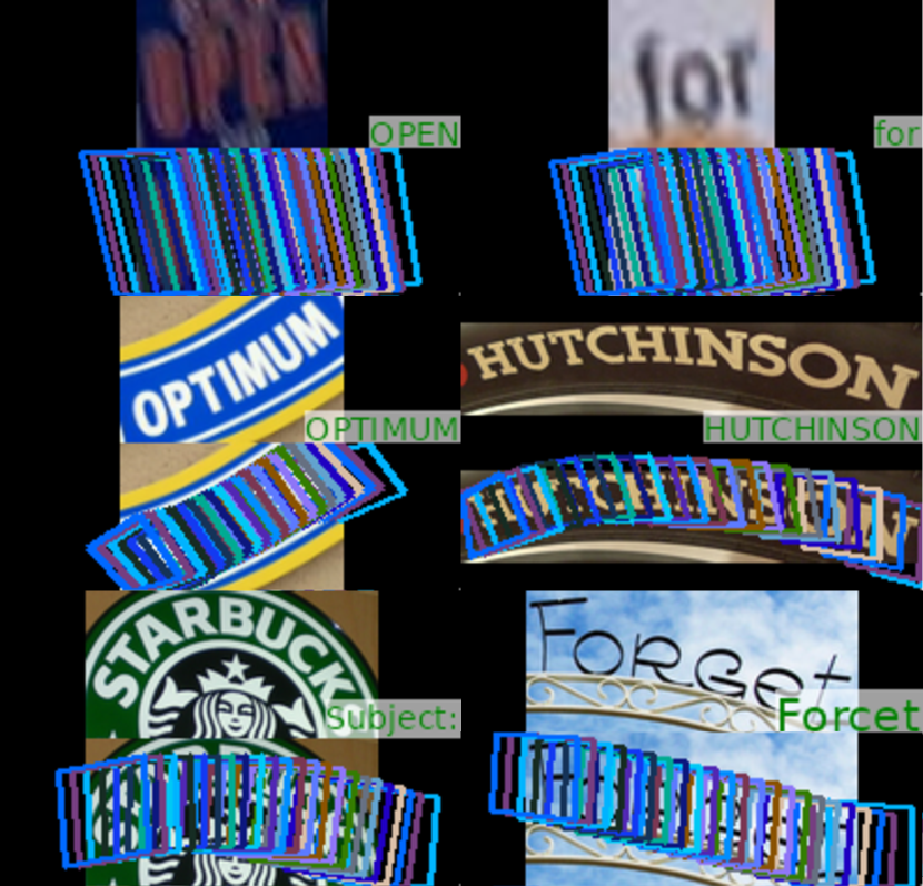
Figure 3: Qualitative evaluation of our approach. We always show the input image with the predicted word and also the predicted regions of interest, below the input image. The last row shows two failure cases of our model.

4.1 Datasets

We train our model only on publicly available synthetic datasets. Our model is evaluated on each benchmark dataset without further fine-tuning. For training we use the following datasets: MJSynth [11], SynthText in the Wild [5], and SynthAdd [17]. We evaluate our model on the following datasets: ICDAR 2013 (IC13) [15], ICDAR2015 (IC15) [14], IIIT5K-Words (IIIT5K) [23], Street View Text (SVT) [37], Street View Text Perspective (SVTP) [26], and CUTE80 (CUTE) [27]. In the following, we shortly introduce each dataset:

Training Datasets

We train our model on publicly available datasets, in order to allow a fair comparison of our model to other models. We use MJSsynth [11], which consists of 9 million synthetic word images, SynthText in the Wild [5], which consists of 8 million word images, and SynthAdd [17], which consists of 1.6 million word images.

ICDAR 2013 (IC13) [15]

consists of $1095$ word images for evaluation. Those images contain focused scene text. For a fair comparison with other approaches, we remove all images with non-alphanumeric characters, leaving us with $1015$ images for evaluation.

ICDAR 2015 (IC15) [14]

consists of $2077$ word images for evaluation. The images have been captured using Google Glass without the intent to capture scene text, hence they are severely distorted, or blurred. For fair comparison, we also evaluate on the ICDAR2015-1811 (IC15-1811) subset, which only contains alpha numeric characters.

IIIT5K-Words (IIIT5K) [23]

consists of $3000$ word images for evaluation. Most of the word images are horizontal text, but several images also contain curved text instances.

Street View Text (SVT) [37]

consists of $647$ word images for evaluation, most of which are horizontal text lines, but many images are severely blurred or of bad quality.

Street View Text Perspective (SVTP) [26]

consists of $645$ word images for evaluation. These images have been collected from Google StreetView and contain images with a high rate of distortions.

CUTE80 (CUTE) [27]

consists of $288$ word images for evaluation. The images are mostly of high quality but contain a lot of curved text instances.

4.2 Implementation Details

We implemented our model using Chainer [35], and based our implementation of the transformer for Chainer on [16]. We perform all of our experiments on a NVIDIA GTX 1080Ti GPU. We use RAdam [20] as optimizer, and set the initial learning rate to $10^{-4}$. We multiply the learning rate by $0.1$ at each new epoch. We train our model for about 3 epochs, use a batch size of $32$, and resize the input images to $200\times 64$, while maintaining the aspect ratio. The output of the localization network is set to be image crops of size $50\times 64$, which is also used as input size for the recognition network. Our model is trained from scratch with randomly initialized weights and we use GroupNormalization [40] instead of BatchNormalization [10] throughout the network. We follow [36] when setting the hyperparameters of the transformer, but we use only one layer of encoder and decoder instead of six. During training we use gradient clipping in the localizer to avoid divergence of the network. We use some data augmentation during training of our model and augment $40\text{\,}\mathrm{\char 37\relax}$ of the input images, by randomly resizing them, adding some blur, and adding some extra distortion. During test time, following [38], we also perform some data augmentation. We rotate each input image by $\pm 5$ degrees, if the width is $1.3$ times larger than the height, otherwise we rotate the image by $\pm 90$ degrees. We then put all rotated images and the original image into the network. We use the prediction with the highest average score for each character as output of our network.

4.3 Comparison with State-of-the-art

Method	IC13	IC15	IC15-1811	IIIT5K	SVT	SVTP	CUTE
Jaderberg et al. 2014 [11]	$90.8$	-	-	-	$80.7$	-	-
Shi et al. 2016 [28]	$89.6$	-	-	$81.2$	$82.7$	-	-
Shi et al. 2016 [29]	$88.6$	-	-	$81.9$	$81.9$	-	-
Liu et al. 2018 [21]	$91.1$	74.2	-	$92.0$	$85.5$	$78.9$	-
Cheng et al. 2018 [4]	-	$68.2$	-	$87.0$	$82.8$	$73.0$	$76.8$
Bai et al. 2018 [2]	94.4	-	$73.9$	$88.3$	$85.9$	-	-
Shi et al. 2019 [30]	$91.8$	-	$76.1$	$93.4$	$89.5$	$78.5$	$79.5$
Wang et al. 2019 [39]	-	-	-	$90.5$	$82.2$	-	$83.3$
Li et al. 2019 [17]	$91.0$	$69.2$	-	$91.5$	$84.5$	$76.4$	$83.3$
Luo et al. 2019 [22]	$92.4$	$68.8$	-	$91.2$	$88.3$	$76.1$	$77.4$
Liao et al. 2019 [19]	$91.5$	-	-	$91.9$	$86.4$	-	$79.9$
Wang et al. 2019 [38]	$92.0$	74.8	79.1	94.2	$89.0$	$81.7$	$83.7$
Zhan & Lu 2019 [41]	$91.3$	-	$76.9$	$93.3$	90.2	$79.6$	$83.3$
Liao et al. 2019 [18]	95.3	-	$77.3$	$93.9$	90.6	82.2	87.8
KISS (Ours)	$93.1$	74.2	80.3	94.6	$89.2$	83.1	89.6

Table 1: Results of our model compared to other proposed models. Numbers in bold font and italic font indicate the best and second-best performance, respectively. We only report results that are obtained without any lexicon. It is possible to see that our model outperforms every other model on irregular text datasets, showing the general robustness to distortions of our model.

We compare our model with several other methods on the datasets introduced in Section 4.1. For a fair comparison we always show the results that were obtained using only synthetic data and without an ensemble of multiple models (where known). We show the results of our best performing model (exactly the model described in Section 3) in Table 1. Our method, although without any components tailored to the task of scene text recognition, reaches state-of-the-art results on four of the seven benchmarks and reaches competitive results on the other three benchmarks. We note that we can not evaluate our model on the entire ICDAR2015 dataset, since this dataset contains a range of characters we did not train our model for. This accounts for about $1.8\text{\,}\mathrm{\char 37\relax}$ of the images in the ICDAR2015 dataset. Even though we did not use building blocks specifically tailored to the task of scene text recognition, we are still able to achieve state-of-the-art results. We are still wondering, why this is the case. In our ablation study (Section 4.4) we try to show which building blocks of our network boost the performance of our network the most, but it still does not answer the question, why our method outperforms other methods. In our future work, we will investigate this further. In Figure 3, we show some qualitative results of our approach. It is possible to see that our model works well on distorted and heavily blurred text. The failure cases show that our model is not able to handle heavily curved text well, this might be because the training dataset lacks this kind of image for training.

4.4 Ablation Study

Variation	IC13	IC15	IC15-1811	IIIT5K	SVT	SVTP	CUTE
SynthText only	90.4	65.8	71.1	89.2	82.4	73.3	74.7
Balanced dataset	91.8	72.5	77.6	93.1	86.7	77.3	89.2
Transformer Localizer	91.0	70.6	76.3	92.5	87.9	78.0	85.8
Softmax Recognizer	86.0	54.7	59.4	82.2	74.6	60.1	68.4
$\text{Transformer}^{2}$ w/o Augmentation	93.0	72.8	75.3	90.8	88.3	79.8	85.4
Recognition Network only	90.9	67.5	73.6	91.5	85.0	74.6	78.1
Without Augmentation	92.7	72.9	75.4	90.8	88.3	79.2	87.2
Recognizer Optimizer	92.5	73.4	77.0	94.5	90.0	79.8	87.2
KISS	93.1	74.2	80.3	94.6	89.2	83.1	89.6

Table 2: Results of our ablation experiments. Bold font indicates the best performance for the corresponding dataset.

Besides the comparison with state-of-the-art methods, we also perform a range of experiments where we make changes to several building blocks of our network or changes to the way we train the network. With these experiments we want to determine the performance impact of those changes and also which building blocks are important for a state-of-the-art scene text recognition model. The results of our ablation experiments can be seen in Table 2. We performed the following ablation experiments:

Training Data

In the first experiment, we do not use all datasets as described in Section 4.1, but only the SynthText dataset [5], which includes about $41\text{\,}\mathrm{\char 37\relax}$ of the overall training images. With this experiment we want to determine the impact a reduced amount of training data has on our model. The result (SynthText only) shows that reducing the amount of training data has a drastic impact on performance, indicating that using only one of the synthetic datasets is not enough to train a well balanced model. We also perform an experiment where we balance the training dataset. Here, we take all three synthetic datasets and only keep a maximum of $200\,000$ samples per word-length. This leaves us with about $60\text{\,}\mathrm{\char 37\relax}$ of the overall training images. The result for this experiment (Balanced dataset) shows that this does not decrease the performance of the model as drastically, as using only the SynthText dataset does, which shows that all three datasets together contain a well balanced range of examples and allow the model to better generalize to real-world examples.

Changes to the network architecture

In this series of experiments, we exchange several building blocks of our network architecture and observe the impact of these changes. First, we exchange the LSTM in the localization network with a transformer. Here we want to answer two questions: (1) is it possible to train a transformer without immediately providing the labels in the forward pass? (2) Does a transformer based localizer increase the performance of the model, especially on heavily distorted images? The results (Transformer Localizer) show that it is indeed possible to train a transformer without the need to provide labels in the forward pass, but we note that it takes significantly longer than training a RNN, because the full sequence has to be created step by step. We also see from the results that a transformer based localizer does not increase the performance of the model, hence a transformer does not provide much value at this stage of the network. We note that we are currently not enabling the transformer to attend to a two dimensional feature map. Doing so could improve the results we could achieve using a localization network with a transformer, we leave that open for future work. The second experiment we conduct, is to exchange the transformer in the recognition network with a plain softmax classifier, as it is used in [11]. The result (Softmax Recognizer) shows that using a sequence to sequence model with attention (in our case a transformer) is indeed one of the most important building blocks for a successful text recognition model. Next, we increase the number of transformer layers of the transformer in the recognition network. The result ($\text{Transformer}^{2}$ w/o Augmentation) shows that this change leads to similar performance than without this change, hence it is sufficient to stay with the simpler approach. The last experiment is to train the model without the localization network on regularly cropped regions of interest. The result (Recognition Network only) shows that our model performs very good on datasets that contain focused scene text. On datasets that do not contain focused scene text or a lot of curved text instances, this model is outperformed by our proposed model. This shows that a careful selection of regions of interest is important for the network to succeed, which confirms the observations by [29, 30, 41], where they argue that rectification is beneficial for the task of scene text recognition.

Changes to the Training Method

In our last series of experiments, we experiment with different ways of training the model. First, we train the model without data augmentation. From the result (Without Augmentation), we can see that data augmentation is crucial for achieving a good result on several datasets, while on other datasets, augmentation does not seem to have a large impact. This shows that our current augmentation strategy is suited very well for the data in some datasets and also supports the findings of our first ablation experiments, showing that training data is a crucial factor for a very good performance. Another change we made to the training methodology is to add an extra optimizer that only trains the recognition network on regularly cropped slices of a word image. The rationale behind this idea is, that this extra training might help the recognition network to perform better, as it sees more diverse input data and also better cropped regions of interest, since the start of the training. However, the results (Recognizer Optimizer) show that this is not the case. Using this training methodology also does not decrease the performance of the model by a large margin.

5 Conclusion

In this paper, we have presented KISS, a neural network for scene text recognition that only consists of off-the-shelf neural network building blocks. Our model architecture is simple and can be trained end-to-end from scratch. We also presented methods to successfully train a model with a spatial transformer, but without the need for careful parameter initialization. In our experiments, we showed that our model reaches competitive/state-of-the-art results compared to other approaches. Our results show that it is possible to reach state-of-the-art performance, using only off-the-shelf neural network components. In our ablation study we showed that using a sequence-to-sequence model with attention and the availability of diverse training data are the most important factors for creating a state-of-the-art model for scene text recognition. But, these results still do not answer the question why our method performs better than others. In the future, we would like to investigate this further and show which modules are the most important ones for the task of scene text recognition.

References

- [1] Dzmitry Bahdanau, Kyunghyun Cho, and Yoshua Bengio. Neural machine translation by jointly learning to align and translate. In 3rd International Conference on Learning Representations, ICLR 2015, San Diego, CA, USA, May 7-9, 2015, Conference Track Proceedings, 2015.
- [2] Fan Bai, Zhanzhan Cheng, Yi Niu, Shiliang Pu, and Shuigeng Zhou. Edit Probability for Scene Text Recognition. In Proceedings of the IEEE Conference on Computer Vision and Pattern Recognition, pages 1508–1516, 2018.
- [3] Christian Bartz, Haojin Yang, and Christoph Meinel. SEE: Towards Semi-Supervised End-to-End Scene Text Recognition. In Thirty-Second AAAI Conference on Artificial Intelligence, Apr. 2018.
- [4] Zhanzhan Cheng, Yangliu Xu, Fan Bai, Yi Niu, Shiliang Pu, and Shuigeng Zhou. AON: Towards Arbitrarily-Oriented Text Recognition. In Proceedings of the IEEE Conference on Computer Vision and Pattern Recognition, pages 5571–5579, 2018.
- [5] Ankush Gupta, Andrea Vedaldi, and Andrew Zisserman. Synthetic Data for Text Localisation in Natural Images. In Proceedings of the IEEE Conference on Computer Vision and Pattern Recognition, pages 2315–2324, 2016.
- [6] Kaiming He, Georgia Gkioxari, Piotr Dollar, and Ross Girshick. Mask R-CNN. In Proceedings of the IEEE International Conference on Computer Vision, pages 2961–2969, 2017.
- [7] Kaiming He, Xiangyu Zhang, Shaoqing Ren, and Jian Sun. Deep residual learning for image recognition. In Proceedings of the IEEE Conference on Computer Vision and Pattern Recognition, pages 770–778, 2016.
- [8] Pan He, Weilin Huang, Yu Qiao, Chen Change Loy, and Xiaoou Tang. Reading scene text in deep convolutional sequences. In Proceedings of the Thirtieth AAAI Conference on Artificial Intelligence, pages 3501–3508. AAAI Press, 2016.
- [9] S. Hochreiter and J. Schmidhuber. Long Short-Term Memory. Neural Computation, 9(8):1735–1780, Nov. 1997.
- [10] Sergey Ioffe and Christian Szegedy. Batch Normalization: Accelerating Deep Network Training by Reducing Internal Covariate Shift. In Proceedings of the 32Nd International Conference on International Conference on Machine Learning - Volume 37, ICML’15, pages 448–456, Lille, France, 2015. JMLR.org.
- [11] M. Jaderberg, K. Simonyan, A. Vedaldi, and A. Zisserman. Synthetic Data and Artificial Neural Networks for Natural Scene Text Recognition. In Workshop on Deep Learning, NIPS, 2014.
- [12] Max Jaderberg, Karen Simonyan, Andrew Zisserman, and Koray Kavukcuoglu. Spatial Transformer Networks. In Advances in Neural Information Processing Systems 28, pages 2017–2025. Curran Associates, Inc., 2015.
- [13] Max Jaderberg, Andrea Vedaldi, and Andrew Zisserman. Deep Features for Text Spotting. In Computer Vision – ECCV 2014, number 8692 in Lecture Notes in Computer Science, pages 512–528. Springer International Publishing, Sept. 2014.
- [14] D. Karatzas, L. Gomez-Bigorda, A. Nicolaou, S. Ghosh, A. Bagdanov, M. Iwamura, J. Matas, L. Neumann, V. R. Chandrasekhar, S. Lu, F. Shafait, S. Uchida, and E. Valveny. ICDAR 2015 competition on Robust Reading. In 2015 13th International Conference on Document Analysis and Recognition (ICDAR), pages 1156–1160, Aug. 2015.
- [15] Dimosthenis Karatzas, Faisal Shafait, Seiichi Uchida, Masakazu Iwamura, Lluis Gomez i Bigorda, Sergi Robles Mestre, Joan Mas, David Fernandez Mota, Jon Almazan Almazan, and Lluis Pere de las Heras. ICDAR 2013 robust reading competition. In 2013 12th International Conference on Document Analysis and Recognition, pages 1484–1493. IEEE, 2013.
- [16] Guillaume Klein, Yoon Kim, Yuntian Deng, Jean Senellart, and Alexander M. Rush. OpenNMT: Open-source toolkit for neural machine translation. In Proc. ACL, 2017.
- [17] Hui Li, Peng Wang, Chunhua Shen, and Guyu Zhang. Show, Attend and Read: A Simple and Strong Baseline for Irregular Text Recognition. Proceedings of the AAAI Conference on Artificial Intelligence, 33:8610–8617, July 2019.
- [18] Minghui Liao, Pengyuan Lyu, Minghang He, Cong Yao, Wenhao Wu, and Xiang Bai. Mask TextSpotter: An End-to-End Trainable Neural Network for Spotting Text with Arbitrary Shapes. IEEE Transactions on Pattern Analysis and Machine Intelligence, pages 1–1, 2019.
- [19] Minghui Liao, Jian Zhang, Zhaoyi Wan, Fengming Xie, Jiajun Liang, Pengyuan Lyu, Cong Yao, and Xiang Bai. Scene Text Recognition from Two-Dimensional Perspective. Proceedings of the AAAI Conference on Artificial Intelligence, 33:8714–8721, July 2019.
- [20] Liyuan Liu, Haoming Jiang, Pengcheng He, Weizhu Chen, Xiaodong Liu, Jianfeng Gao, and Jiawei Han. On the Variance of the Adaptive Learning Rate and Beyond. arXiv:1908.03265 [cs, stat], Aug. 2019.
- [21] Wei Liu, Chaofeng Chen, and Kwan-Yee K. Wong. Char-Net: A Character-Aware Neural Network for Distorted Scene Text Recognition. In Thirty-Second AAAI Conference on Artificial Intelligence, Apr. 2018.
- [22] Canjie Luo, Lianwen Jin, and Zenghui Sun. MORAN: A Multi-Object Rectified Attention Network for scene text recognition. Pattern Recognition, 90:109–118, June 2019.
- [23] Anand Mishra, Karteek Alahari, and Cv Jawahar. Scene Text Recognition using Higher Order Language Priors. In BMVC 2012-23rd British Machine Vision Conference, pages 127.1–127.11. British Machine Vision Association, 2012.
- [24] L. Neumann and J. Matas. Real-time scene text localization and recognition. In 2012 IEEE Conference on Computer Vision and Pattern Recognition (CVPR), pages 3538–3545, June 2012.
- [25] Eric Partridge. The Routledge Dictionary of Modern American Slang and Unconventional English. Taylor & Francis, 2009.
- [26] Trung Quy Phan, Palaiahnakote Shivakumara, Shangxuan Tian, and Chew Lim Tan. Recognizing Text with Perspective Distortion in Natural Scenes. In Proceedings of the IEEE International Conference on Computer Vision, pages 569–576, 2013.
- [27] Anhar Risnumawan, Palaiahankote Shivakumara, Chee Seng Chan, and Chew Lim Tan. A robust arbitrary text detection system for natural scene images. Expert Systems with Applications, 41(18):8027–8048, Dec. 2014.
- [28] Baoguang Shi, Xiang Bai, and Cong Yao. An end-to-end trainable neural network for image-based sequence recognition and its application to scene text recognition. IEEE Transactions on Pattern Analysis and Machine Intelligence, 2016.
- [29] Baoguang Shi, Xinggang Wang, Pengyuan Lyu, Cong Yao, and Xiang Bai. Robust Scene Text Recognition With Automatic Rectification. In Proceedings of the IEEE Conference on Computer Vision and Pattern Recognition, pages 4168–4176, 2016.
- [30] Baoguang Shi, Mingkun Yang, Xinggang Wang, Pengyuan Lyu, Cong Yao, and Xiang Bai. ASTER: An Attentional Scene Text Recognizer with Flexible Rectification. IEEE Transactions on Pattern Analysis and Machine Intelligence, 41(9):2035–2048, Sept. 2019.
- [31] Xingjian SHI, Zhourong Chen, Hao Wang, Dit-Yan Yeung, Wai-kin Wong, and Wang-chun WOO. Convolutional LSTM Network: A Machine Learning Approach for Precipitation Nowcasting. In C. Cortes, N. D. Lawrence, D. D. Lee, M. Sugiyama, and R. Garnett, editors, Advances in Neural Information Processing Systems 28, pages 802–810. Curran Associates, Inc., 2015.
- [32] K. Simonyan and A. Zisserman. Very Deep Convolutional Networks for Large-Scale Image Recognition. In International Conference on Learning Representations, 2015.
- [33] Nitish Srivastava, Geoffrey E Hinton, Alex Krizhevsky, Ilya Sutskever, and Ruslan Salakhutdinov. Dropout: A simple way to prevent neural networks from overfitting. Journal of machine learning research, 15(1):1929–1958, 2014.
- [34] Christian Szegedy, Wei Liu, Yangqing Jia, Pierre Sermanet, Scott E. Reed, Dragomir Anguelov, Dumitru Erhan, Vincent Vanhoucke, and Andrew Rabinovich. Going deeper with convolutions. In IEEE Conference on Computer Vision and Pattern Recognition, CVPR 2015, Boston, MA, USA, June 7-12, 2015, pages 1–9, 2015.
- [35] Seiya Tokui, Kenta Oono, Shohei Hido, and Justin Clayton. Chainer: A Next-Generation Open Source Framework for Deep Learning. In Proceedings of Workshop on Machine Learning Systems (LearningSys) in The Twenty-Ninth Annual Conference on Neural Information Processing Systems (NIPS), 2015.
- [36] Ashish Vaswani, Noam Shazeer, Niki Parmar, Jakob Uszkoreit, Llion Jones, Aidan N Gomez, Łukasz Kaiser, and Illia Polosukhin. Attention is All you Need. In I. Guyon, U. V. Luxburg, S. Bengio, H. Wallach, R. Fergus, S. Vishwanathan, and R. Garnett, editors, Advances in Neural Information Processing Systems 30, pages 5998–6008. Curran Associates, Inc., 2017.
- [37] Kai Wang, B. Babenko, and S. Belongie. End-to-end scene text recognition. In 2011 International Conference on Computer Vision, pages 1457–1464, Nov. 2011.
- [38] Peng Wang, Lu Yang, Hui Li, Yuyan Deng, Chunhua Shen, and Yanning Zhang. A Simple and Robust Convolutional-Attention Network for Irregular Text Recognition. arXiv:1904.01375 [cs], Apr. 2019.
- [39] Qingqing Wang, Wenjing Jia, Xiangjian He, Yue Lu, Michael Blumenstein, and Ye Huang. FACLSTM: ConvLSTM with Focused Attention for Scene Text Recognition. arXiv:1904.09405 [cs], Apr. 2019.
- [40] Yuxin Wu and Kaiming He. Group normalization. In Computer Vision - ECCV 2018 - 15th European Conference, Munich, Germany, September 8-14, 2018, Proceedings, Part XIII, pages 3–19, 2018.
- [41] Fangneng Zhan and Shijian Lu. ESIR: End-To-End Scene Text Recognition via Iterative Image Rectification. In Proceedings of the IEEE Conference on Computer Vision and Pattern Recognition, pages 2059–2068, 2019.