Evaluation of performance portability frameworks for the implementation of a particle-in-cell code

Abstract

This paper reports on an in-depth evaluation of the performance portability frameworks Kokkos and RAJA with respect to their suitability for the implementation of complex particle-in-cell (PIC) simulation codes, extending previous studies based on codes from other domains. At the example of a particle-in-cell model, we implemented the hotspot of the code in C++ and parallelized it using OpenMP, OpenACC, CUDA, Kokkos, and RAJA, targeting multi-core (CPU) and graphics (GPU) processors. Both, Kokkos and RAJA appear mature, are usable for complex codes, and keep their promise to provide performance portability across different architectures. Comparing the obtainable performance on state-of-the art hardware, but also considering aspects such as code complexity, feature availability, and overall productivity, we finally draw the conclusion that the Kokkos framework would be suited best to tackle the massively parallel implementation of the full PIC model.

1 Introduction

Modern high-performance computing (HPC) systems are getting increasingly complex, in particular concerning the hardware architecture of the clusters’ nodes. This trend is reflected in the development of the “Top 500” ranking of the fastest supercomputers [1], where a growing fraction of HPC systems deploys various types of accelerators or coprocessors, in addition to the prevailing multi-core CPUs. As of November 2018, such accelerated systems contribute a total (peak-performance weighted) share of about 40% within the Top 500 [1] list, with more than two dozens of different types of accelerators (GPUs in the majority of systems). For an individual HPC system, in particular at the high end of the list, GPUs contribute a large fraction of the nominal peak performance.

While for handling inter-node communication the Message Passing Interface (MPI [2]) remains unchallenged as the programming model which has proven stable, reliable, portable, and well supported over more than 25 years, a de-facto standard for programming heterogeneous compute nodes has yet to emerge. The situation is quite adequately described by the term “MPI + X” which has been around for a number of years [3], but today, the “X” still represents a variety of node-level programming paradigms which are mostly specific for a certain type of hardware, or even vendor.

With OpenMP[4], OpenACC[5], and OpenCL[6], to name the most relevant and widespread ones, there is a set of language extensions to C and Fortran available that— at least partly—offer portable programming across various types of compute nodes: OpenMP[4] has been very successful for programming multi-core CPUs, and most recent specifications target also accelerators. However, there is currently only very limited compiler support for accelerators, and some of the semantics differ between CPUs and accelerators.

Conceptually similar to OpenMP, OpenACC[5] was designed as a high-level, directive-based approach to GPU programming and has been quite successful, in particular as an alternative to CUDA, but also supporting multi-core processors. In practice, however, there is only limited compiler support for OpenACC (proprietary compilers by PGI and CRAY, and experimental support in GCC). For complex application codes, both, the OpenMP, and—maybe to a slightly lesser degree—the OpenACC-based approach likely require target-specific adaptations of data structures and flow control in order to achieve good performance on both, CPUs and GPUs.

OpenCL[7, 6] was designed for heterogeneous systems with CPUs and GPUs, but, in practice, has limited support by compilers and runtimes. Moreover, it exposes many of the complexities of the GPU hardware architecture to its programming model. In particular, parallelism is expressed in the form of so-called kernels which are mapped to the CPU’s or GPU’s threads in a SIMT or SIMD fashion. This often poses severe challenges to HPC codes which typically express parallelism in loops or—more fashionably—in complex task graphs, both of which requires a major rewriting of code, and, for Fortran programs, the construction of C interfaces.

In the absence of a de-facto standard for achieving portable performance, scientific HPC application development, especially when targeting high-end machines, is facing an enormous challenge. In practice multiple code versions, code paths, or alike, need to be implemented for the same algorithm, employing different node-level programming models specialized for the target hardware platforms. Applying advanced software engineering techniques, some of the complexity can be encapsulated in certain “lower” layers of the software architecture of an application (e.g. in a custom domain-specific language [8, 9]), but readability, maintainability, and sustainability of such code is often significantly impacted.

Hence, there is significant demand and motivation to develop tools for abstracting the source code from the hardware. Performance portability frameworks enable programmers to target multiple architectures, ideally achieving good performance on any of them without the need to implement and optimize individually. Existing frameworks typically build upon the C++ programming language with templates (ideally, architecture-dependent decisions are taken automatically at compile time) and provide a limited set of building blocks for parallelism while hiding the complexity of the target architecture from the application programmer. The promise is that a single source code can run efficiently on multiple architectures. Following the paradigm of “separation of concerns” the framework eventually delegates compilation and execution to well-established “native” programming models and runtimes, such as the aforementioned OpenMP (for multi-core CPUs), or the proprietary CUDA model (for NVIDIA GPUs). Those “backends” can be implemented and maintained by specialists in an application-agnostic way and thus become transparent for the application programmer. For a more comprehensive review on options for performance portability we refer to the introduction of Ref. [10] and the references therein.

In this paper, we shall focus on Kokkos [11] and RAJA [12] which, at the time of writing, are the two leading C++ performance portability frameworks. Both use advanced meta-programming techniques to generate architecture-specific code and optimizations at compile time and are freely available as open source under BSD-type licenses. Similar, though still in beta state and therefore not considered currently, is the alpaka performance portability library[13, 14]. It provides hardware abstraction to support single-source accelerator development. Specifically, this paper reports on our experiences with employing Kokkos and RAJA for achieving performance portability of a complex particle-in-cell (PIC) code across various types of multi-core and GPU-accelerated HPC platforms, and compares it to platform-optimized versions of the code. In addition to the computational performance, our assessment considers aspects such as code complexity, feature availability, and overall productivity of the approach.

The paper is structured as follows. Subsection 1.1 gives a brief review of related work on the assessment of performance-portability frameworks. Next, subsection 1.2 introduces the methodology and the goals of the present work and subsection 1.3 briefly introduces the numerical model of our study. In section 2, we briefly summarize the main concepts of Kokkos and RAJA and put them into context by means of code examples from our application. We then turn towards a usability review of both frameworks in section 3, before we report in detail on the performance achieved on state-of-the art CPU and GPU nodes in section 4. Finally, the paper closes with a summary and conclusions in section 5.

1.1 Related work

To our knowledge, there exist only few comparisons of Kokkos, RAJA, and other parallel frameworks at the level of a complex HPC application.

Martineau et al. did a comparison of Kokkos, RAJA, OpenACC, OpenMP 4.0, CUDA, and OpenCL based on the Tealeaf application, a miniapp solving the heat conduction equation using finite differences[15, 16]. The authors report a 5% to 30% performance penalty for Kokkos and RAJA compared to architecture-specific implementations.

Sunderland et al. report on the Kokkos refactoring of the large legacy code base Uintah, used to model turbulent combustion [17]. In their case, the introduction of Kokkos views and proper memory layouts even increased the performance of specific kernels thanks to more efficient memory accesses and vectorization.

More recently, Demeshko et al. report specifically on a Kokkos port of parts of the complex finite element framework Albany in great detail[10]. They focus on the refactoring process, and present performance comparisons on the target platforms CPU, GPU, and KNL, though a baseline defined by the original code’s performance before the porting is lacking.

1.2 Methodology

We consider a complex HPC application from the plasma physics domain, based on a numerical model which solves the Vlasov–Maxwell system of equations using a Particle-In-Cell (PIC) method[18]. The fact that a full-scale implementation of the code has yet to be developed and optimized for state-of-the-art HPC systems, which is a multi person-year effort, served as the main motivation for the pilot-study and assessment of portability frameworks presented here.

As a baseline implementation, we extracted a generic part from the original FORTRAN implementation taken from SeLaLib [19] and rewrote it in C++. Starting out from this code, six different parallel versions were developed, namely, using plain OpenMP directives, plain OpenACC directives, plain CUDA, Kokkos, hybrid OpenMP/Kokkos, and RAJA. The baseline version and the six parallel versions, targeting multi-core and graphics processors, were extensively benchmarked, and are compared with respect to their performance. In addition, we address soft factors such as the programmers’ productivity, the code complexity, and the overall experience.

Since the fundamental computational kernels of the PIC method are somewhat complementary to the patterns encountered in finite-element methods or mesh-based domain-decomposition schemes that were targeted in the aforementioned studies, our assessment may serve as another major building block for judging the relevance of portability frameworks for HPC application development as a whole.

1.3 Numerical model

The particle-in-cell method solves a hyperbolic conservation law by representing a distribution function by macro-particles that evolve in a Lagrangian frame along the characteristic equations accociated with the conservation law. These macro-particles are represented by their position in phase space and a weight. Often the particle description is coupled to a field description of some moments of the distribution function. We study the solution of the Vlasov–Maxwell equations in six-dimensional phase space. The Vlasov equation models the evolution of a species $s$ of a plasma in its self-consistent and external electromagnetic fields

$$\partial_{t}f_{s}(\textbf{x},\textbf{v},t)+\textbf{v}\cdot\nabla_{\textbf{x}}f_{s}(\textbf{x},\textbf{v},t)+\frac{q_{s}}{m_{s}}\left(\textbf{E}(\textbf{x},t)+\textbf{v}\times\textbf{B}(\textbf{x},t)\right)\cdot\nabla_{\textbf{v}}f_{s}(\textbf{x},\textbf{v},t)=0,$$ (1)

where $f$ denotes the distribution function, E the electric, and B the magnetic field, and $q_{s}$ and $m_{s}$ the charge and mass of the particles, respectively. The self-consistent fields can be computed from Maxwell’s equations

$$\frac{\partial\textbf{E}}{\partial t}-\nabla\times\textbf{B}=-\textbf{j},\quad$$ (2a)

$$\frac{\partial\textbf{B}}{\partial t}+\nabla\times\textbf{E}=0,$$ (2b)

$$\nabla\textbf{E}=\rho,\quad$$ (2c)

$$\nabla\textbf{B}=0,$$ (2d)

where $\rho$ and j denote the charge and current density, respectively, which are defined as velocity moments of the distribution functions,

$$\rho=\sum_{s}q_{s}\int f_{s}\text{d}\textbf{v},\text{ and }\textbf{j}=\sum_{s}q_{s}\int\textbf{v}f_{s}\text{d}\textbf{v}.$$ (3)

Particle methods represent the distribution function $f_{s}$ by a large number of macroparticles that are defined by their position $(\textbf{x}_{p},\textbf{v}_{p})$ in six-dimensional phase space and a (constant) weight, and evolve over time. The fields are represented on a grid by some discretization method.

In our case study, we follow the geometric electromagnetic particle-in-cell (GEMPIC) scheme as proposed in [18] where the fields are represented by conforming spline finite elements as proposed in [20]. The common parallel structure of the particle-in-cell method are particle loops which are embarrassingly parallel but assemble and evaluate grid-based quantities that are shared between several processes and thus require a reduction step (and the solution of the field equations) following the particle loop. Our implementation focuses of a subset of equations, namely a particle loop that identifies the position of the particle in the grid, evaluates the magnetic field at the particle position, updates $x_{1,p}$ and $v_{2,p}$, $v_{3,p}$, and accumulates the first component of the current density. The particle loop is then followed by a reduction of the current density. Appendix A gives a more detailed description of the implemented method. Moreover, we refer to [18] where this subset of instructions is presented as the operator $H_{p_{1}}$.

Although the study uses a particular operator stemming from the GEMPIC discretization, we believe that the findings are general enough to apply to other types of particle-in-cell schemes. Note that we focus in the present work only on shared-memory parallelization with a simple data structure storing particle position, velocity, and weight in an array-of-structures data type. Including advanced data types that enable vectorization and efficient data access (cf. e.g. Ref. [21]) and adapting them to the special requirement of the current-deposition loop as it appears in the GEMPIC equations is a different topic which we do not address in this work.

2 Performance Portability Frameworks

The aim of performance portability frameworks like Kokkos and RAJA is to enable scientific programmers to write generic parallel code that can be compiled and run on several parallel architectures while minimizing or even eliminating the need to implement architecture-specific code. At the same time, nearly the same computational performance as obtained from an architecture-specific implementation is supposed to be achieved. Thus, the application programmer has to take care of only a single code version and is shielded from technical details of different target architectures. Moreover, the code is expected to run at high performance also on future HPC hardware, provided that the chosen performance-portability framework is properly maintained.

To point out the concepts, similarities, and differences of Kokkos and RAJA, we present a recap of both frameworks, partly based on code from our implementations of the numerical model. For direct comparison of the source code from the different programming models we have included a color-coded listing in appendix B. These code excerpts transport the essential ideas behind Kokkos and RAJA. We used Kokkos version 2.7.00 and RAJA version 0.6.0 during development work. For further details on the abstractions and the programming models, we refer the reader to the official documentation of Kokkos[22] and RAJA[23].

In the following sections, we will briefly address the role of the individual building blocks for the implementation of our model code. The key feature of both Kokkos and RAJA is to offer abstractions for the memory (organized in so-called views) and the parallel operations. Kokkos defines the following six fundamental abstractions:

1. execution spaces specify on which processor to execute,

2. execution patterns specify the parallel operation (i.e. for, reduction, scan, task),

3. execution policies specify how to execute the pattern,

4. memory spaces specify where to allocate memory and store data,

5. memory layouts control the mapping of indices to physical memory,

6. memory traits specify how to access the memory.

RAJA supports various types of parallel operations, such as loops (for), reductions, atomics (handled by the data structure in Kokkos), and scans, and defines a policy for each of them specifying both where and how the parallel operation is executed. The memory abstraction is through views that wrap the pointer to the actual memory and enable processing of the data independent of its index organization that is defined by the concept of layouts. Note that Kokkos automatically allocates the memory according to the memory space while RAJA requires the user to explicitly define the memory layout for each case. These abstractions enable the implementation of parallel code as outlined in the following.

2.1 Array types and memory management

Kokkos and RAJA both offer multidimensional array primitives called views. These views allow for an abstraction of the storage layout from the data which, most importantly, relieves the programmer from architecture-specific optimization work. For example, on cache-based architectures such as CPUs, it is of advantage to access memory linearly (i.e. multiple consecutive elements from each thread) whereas on GPUs it typically performs better to access memory in a coalesced fashion (i.e. one element only per lightweight thread). Using the view abstraction, the optimal layout and padding can be chosen automatically and individually for each architecture (execution space).

In both frameworks, a view contains only metadata which is stored in host memory, plus a pointer to the actual data that can be located on the host or on the device. Kokkos allocates memory together with views, whereas RAJA does not allocate memory. To be able to, e.g., define an array independent of its location, Kokkos implements the so called HostMirror type. This special view transparently guarantees data access to device memory from the host. In our code, the names of such views contain the keyword _host. With RAJA, managing host and device memory allocation and transfers is the responsibility of the user, similarly to the CUDA heterogeneous programming model.

In the codes presented in the appendix, Kokkos views are used, e.g., in the lines 101-104 of the listing B,

⬇

this->view_j_dofs_local = Kokkos::View<double*>("view_j_dofs_local", this->part_mesh_coupling.view_n_dofs_host(0));

this->view_j_dofs_local_host = Kokkos::create_mirror_view(this->view_j_dofs_local);

⬇

101for(long i=0; i<this->view_j_dofs_local_host.size(); i++) {

102 this->view_j_dofs_local_host(i) = 0.0;

103}

104Kokkos::deep_copy(this->view_j_dofs_local, this->view_j_dofs_local_host);

and RAJA views are used, e.g., in the lines 108-122 of the listing B:

⬇

this->d_j_dofs_local = memoryManager::allocate<double>(this->part_mesh_coupling.n_dofs);

this->raja_j_dofs_local. RajaVector1DType();

new(&this->raja_j_dofs_local) RajaVector1DType(this->d_j_dofs_local, this->part_mesh_coupling.n_dofs);

⬇

108#if defined(RAJA_ENABLE_CUDA) && defined(I_USE_CUDA)

109 RAJA::forall<RAJA::cuda_exec<32>>(RAJA::RangeSegment(0, this->part_mesh_coupling.n_dofs),

110 [*this] RAJA_DEVICE (int i) {

111 if(i<this->part_mesh_coupling.raja_n_dofs(0)) {

112 this->raja_j_dofs_local(i) = 0.0;

113 }

114 });

115#else

116 RAJA::forall<RAJA::omp_parallel_for_exec>(RAJA::RangeSegment(0, this->part_mesh_coupling.n_dofs),

117 [this] (int i) {

118 if(i<part_mesh_coupling.raja_n_dofs(0)) {

119 raja_j_dofs_local(i) = 0.0;

120 }

121 });

122#endif

2.2 Parallel patterns

Kokkos and RAJA both implement data parallel operations (for, reduce, scan), and Kokkos in addition also a task parallel operation (task). These parallel operations are called patterns in the case of Kokkos, whereas RAJA subsumes them under the term policy, see section 2.3 below, however the concepts are the same. The calls to parallel code can be done via lambda functions in both frameworks. With Kokkos, a functor can be used alternatively to wrap parallel code.

The inputs of the lambda function or the functor have to match the expected input parameters of the execution pattern and policy. This prohibits the use of arguments to pass data, therefore lambda functions seem easier to work with on a small scale. To get access to the data, functors require all the data as class members.

According to our experience, functors are often easier to test and somewhat more readable, especially for source codes with many lines. However, plain functors seem to pose a problem when multiple parallel functions to be accessed via the same functor need to be implemented. To address this, Kokkos uses an Execution Tag. The tag is passed as a template parameter to the execution policy, which will then feed it to the operator(), making the specialization to call a certain internal function a compile-time decision. An execution tag is used at line 176 of Listing B:

⬇

176auto policy = Kokkos::TeamPolicy<pic_routine, ExecSpace>

The first template parameter, pic_routine, is the tag that will define which operator() to use. The second parameter is the execution space defining, at compile time, the information on where to execute the code.

At the time of writing and for both the frameworks, the reduction loop supported on both CPU and GPU only covered scalar reductions. Vector reduction is a crucial feature for the implementation of a PIC method such as the one considered by us in the present paper. While RAJA does not provide a “ready-to-use” solution for vector reduction, Kokkos provides it by the use of a scatter_view. The scatter_view deals with the allocation of per-thread memory for thread-safe access to the vector, see the example below taken from the lines 316, 445 of the listing B. For completeness we have added a call to the contribute function which performs the reduction:

⬇

445ViewScatterAccessType scatter_access = scatter_view.access();

scatter_access(index1d) += view_j1d(i) * splinejk;

⬇

Kokkos::Experimental::contribute(hamiltonian_splitting.view_j_dofs_local, scatter_view);

For RAJA, we have implemented our own vector reduction by using a different view for each particle’s partial result, and summing the partial results at the end. See the example below adapted from lines 200, 447 and 214 of the listing B.

⬇

//RAJA CPU: initialisation of the handmade reduction 2D array

RAJA::kernel<fdPolicy>(RAJA::make_tuple(RAJA::RangeSegment(0, total_num_threads)),

[&,this] (int i_part) {

for(int i=0; i<part_mesh_coupling.n_dofs; i++)

raja_private_raja_array(i_part).raja_handmade_reduce(i) = 0.0;

});

raja_private_raja_array(i_part).raja_handmade_reduce(index1d) += util_raja.raja_j1d(i) * splinejk;

//RAJA: CPU handmade reduction

RAJA::kernel<fdPolicy>(RAJA::make_tuple(RAJA::RangeSegment(0, part_mesh_coupling.n_dofs)),

[&,this] (int i_part) {

for(int i=0; i<total_num_threads; i++)

d_j_dofs_local[i_part] += raja_private_raja_array(i).raja_handmade_reduce(i_part);

});

2.3 Execution policies

To specify how a parallel pattern is executed, Kokkos knows two types of execution policies, the RangePolicy and the TeamPolicy. The range policy simply defines a range of indices on which a function will be called. No assumption can be made about the order of the concurrent execution, and it is not allowed to synchronize the threads. The team policy adds additional features on top of the range policy. It enables hierarchical parallelism and scratch memory. The scratch memory is a very important feature for the present PIC application, as each thread needs private variables to compute updated particle positions, velocities, etc. At line 176 of Listing B, a TeamPolicy, with shared_size bytes per-thread of scratch memory is declared.

⬇

Kokkos::TeamPolicy{...}.set_scratch_size(1,Kokkos::PerThread (shared_size));

RAJA decides on which hardware the code will run based on the template arguments of the policy. The indices for the data-parallel operation are defined using RangeSegments, a RAJA class to define a range $[\![n,m-1]\!]$. Moreover, e.g., ranges with constant strides $\{n,n+m,n+2*m,...\}$ are possible. In line 189 of listing B, we launch a lambda function on the GPU with 256 threads per thread-block on the indices $[\![0,n\_particles-1]\!]$, as shown below.

⬇

RAJA::forall<RAJA::cuda_exec<256>>(RAJA::RangeSegment(0,

this->particles.group[0].n_particles),

[=,*this] RAJA_DEVICE (int i_part){

{operator_RAJA_GPU}

});

These segments can further be combined into lists of segments for more complex access patterns. However, this advanced index management feature is not necessary for our PIC model and has not been tested in this study.

In the following we turn towards a review of the different frameworks, based on our experience from implementing the PIC algorithm.

3 Usability review

3.1 Implementation overview and methodology

In order to compare Kokkos and RAJA with OpenACC and the architecture-specific programming models, we developed multiple versions of the PIC operator.

C++

A standalone C++ reference implementation of the PIC routine was written first. This code includes input/output and driver functions to run, time, and verify the computation, and serves as the starting point for the other codes below.

OpenMP

Starting from the C++ code, we implemented a thread-parallel version for the CPU using plain OpenMP. Results from this code define the baseline to compare to the Kokkos-CPU and RAJA-CPU codes, see below.

Kokkos

Next, the parallel loops from the OpenMP code were refactored using Kokkos and were verified to produce correct results on CPUs and GPUs. In the following, we refer to this version as Kokkos-CPU when run on the CPU with the Kokkos-OpenMP back end, and as Kokkos-GPU when run on the GPU with the Kokkos-CUDA back end, respectively.

OpenMP/Kokkos

Related to the pure Kokkos implementation, we developed a hybrid code version which uses OpenMP directives in combination with Kokkos views, with the motivation to identify the overhead of the pure Kokkos implementation. Moreover, such hybrid codes naturally emerge during code refactoring work.

RAJA

A parallel implementation was developed using RAJA, and verified on CPUs and GPUs. In the following, we refer to this version as RAJA-CPU when run on the CPU with the RAJA-OpenMP back end, and as RAJA-GPU when run on the GPU with the RAJA-CUDA back end, respectively.

CUDA

To define a baseline for Kokkos’ and RAJA’s GPU performance, a plain CUDA version was implemented.

OpenACC

To complement this comparison, a plain OpenACC version was implemented, which runs on the CPU and on the GPU.

To compile all but the last code we used GCC 6.3 and CUDA 9.1 with appropriate library and compiler flags to optimize for the specific hardware. In particular, the flags -O3 -march=native -fopenmp were passed to gcc, and, e.g., the flags -O3 -arch=sm_70 were passed to nvcc with the -arch flag matching the actual GPU architecture, NVIDIA Volta in this example. For Kokkos, e.g., the macro KOKKOS_ARCH="SKX,Volta70" was specified in addition to specify the target platforms, here Intel Skylake CPU and NVIDIA Volta GPU. To compile the OpenACC code we used PGI 19 with the -fast -acc optimization flags and the respective target specialization flags for the CPU (-ta=multicore) and GPU (e.g., -ta=tesla:cc70).

In the following, we discuss the implementation experience with Kokkos and RAJA individually and address soft factors such as code complexity and productivity, before we turn towards performance benchmarks in section 4.

3.2 Kokkos implementation

To perform a refactoring of existing sequential C++ code into parallel Kokkos code, essentially a two-step process is necessary in the most simple case: First, replace legacy C-style array allocations or, similarly, higher-level data structures such as std::vector with Kokkos::View types, and, second, replace for loops with parallel_for and move the loop bodies into functors or lambda functions.

As mentioned previously, Kokkos execution patterns offer two possibilities to run user code in parallel. For the present work, the functor approach was preferred to the lambda functions, allowing for easy testing and leading to well-readable code.

As a feature of convenience and robustness, Kokkos provides a default execution space that will consider architectures in the order CUDA, OpenMP, pthreads, and serial, if available. This default execution space makes it optional to the programmer to specify the architecture onto which the code is going to be deployed. Complex implementations can of course have parallel sections specified to use distinct execution spaces.

Vector reductions are a crucial feature for our application. The Kokkos reference only covers scalar reductions in the documentation, examples, and test files. However, Kokkos provides a ScatterView class under the experimental namespace that can be used to implement vector reductions. It has a slightly different behavior on the CPU and the GPU: On the CPU, the ScatterView class will duplicate its View internally per thread. After the parallel section, the contribute function has to be called explicitly to compute the reduction from all the internal Views. On the GPU, the ScatterView does not duplicate its View, hence, value updates from concurrent threads need to be performed atomically. On present GPU hardware, the atomic add operation is efficiently implemented[24], which makes it a good choice to perform a reduction instead of using variable duplication. The ScatterView class expects a template parameter to request to use the duplication or the atomic access, but there is no default setting. Hence, we specified different template settings for CPU and GPU using a preprocessor macro. In case of the Kokkos framework, this was the only time two versions of a code section (though 2 lines only) had to be implemented.

Lastly, we need some scratch memory for each thread. For the Kokkos implementation, this is simply achieved by declaring all the needed variables inside the parallel section, such that allocation is done per thread. The total size of the scratch memory inside a parallel loop needs to be known before the parallel dispatch is launched, similarly to CUDA shared memory. Different memory levels with different size caps, corresponding to L1 and L2 cache sizes, can be accessed on the CPU, and similarly for shared memory on the GPU.

3.3 RAJA implementation

Turning towards RAJA and the refactoring of existing sequential C++ code, the same two-step process as already discussed with Kokkos is necessary: First, replace array types with RAJA::View types, and, second replace for loops with forall and move the loop bodies into lambda functions. It is the duty of the user to allocate memory for the RAJA views.

A difference to note is that RAJA does not implement defaults, e.g., for architectures, but rather forces the programmer to consider and specify all the necessary settings explicitly. On the source code level this requires branches to specialize for CPU and GPU versions.

Second, RAJA does not support functors for the parallel dispatch but only lambda functions which required to structure the code differently, compared to Kokkos.

As already discussed for the Kokkos implementation, scratch memory is needed, for which RAJA offers an implementation of shared memory on the GPU. On the CPU, we use regular views.

RAJA does not offer ready-to-use vector reductions, however, it was straight forward to implement such reductions based on views.

3.4 Qualitative comparison

Table 1: Qualitative comparison of the programming models based on a subjective ranking on the scale low, medium, high, as experienced by the programmers.

criterion	OpenMP	OpenACC	CUDA	Kokkos	RAJA
code clarity	high	high	low	medium	medium
productivity	high	medium	low	medium	medium
portability	low	medium	low	high	high
performance	high	high	high	high	medium

In the following, a qualitative review on the code complexity, programmer’s productivity, portability, and performance is given, summarized in table 1.

The directive-based OpenMP and OpenACC programming models were the least intrusive when applied to the loops of the PIC routine, starting from the sequential C++ code. Kokkos and RAJA required both significant restructuring of the existing code for the parallel dispatch via functors or lambda functions. CUDA required a comparable amount of rewriting effort, in particular to map the loops onto a CUDA grid of threads and thread blocks. The overhead for OpenMP and OpenACC in terms of lines of code is the smallest, followed by Kokkos. For RAJA, the overhead is about a factor two compared to Kokkos in many places since separate code for CPU and GPU can be necessary. The CUDA version is comparable to the Kokkos code in terms of lines of code.

Concerning the programmer’s productivity, it took a graduate-level C++ programmer about two months to learn and apply the Kokkos framework successfully to implement the PIC routine. RAJA, conceptually similar and tackled with having the knowledge of Kokkos, took about another month. The OpenMP and CUDA implementations were done faster due to previous experience. To develop the OpenACC code, it was necessary to do the implementation in analogy to the CUDA implementation, keeping the correspondence of OpenACC gangs and CUDA thread blocks in mind. Remarkably, Kokkos and RAJA keep their promise of basically providing a GPU version for free based on implementation work mainly done using the CPU. For completeness, we include the performance ranking in table 1 but refer to the following section 4 for details. Moreover, it should be noted that the specification of the target platform in the Kokkos Makefile via the KOKKOS_ARCH variable already enables the use of correct compiler optimization flags for the respective platform, while for the other frameworks the user has to set these flags manually, a procedure which is tedious and prone to errors.

A drawback common to both frameworks, Kokkos and RAJA, is the fact that the hardware-specific code generated at compile time via C++ template meta programming is not accessible to the programmer for inspection. This limitation does not only affect Kokkos and RAJA, but is well-known to any C++ programmer who uses templates. There is no way to obtain the resulting code in the high-level C++ or C++/CUDA language, rather the programmer has to work at the level of assembly code.

3.5 Hybrid OpenMP/Kokkos

Even though performance portability frameworks enable portability of the code, they often come with a certain overhead which we have also observed in our application (cf. the following section). For this reason, we were interested in the question whether this overhead is intimately connected to the data structures or rather to the implementation. For this reason, we have modified the Kokkos code such that it uses OpenMP parallel for directives instead of the Kokkos loops but keeps the Kokkos views as array objects.

Because Kokkos does reference counting, accessing a regular view from a pure OpenMP parallel section would cause significant overhead. In particular, any operation on a view would be an atomic operation. If one wants to use a view from conventional OpenMP parallel code, the trait of the view needs to be set to Unmanaged. This is what we used for the hybrid OpenMP/Kokkos code, see e.g. the lines 13 and 136 of listing B:

⬇

ViewVector2DUnmanagedType view_particle_array_unmanaged;

this->view_i_weight_unmanaged = this->view_i_weight;

With these modifications it was possible to eliminate the overhead for Kokkos as will be reported on in the next section. We did not perform such an experiment for RAJA. However, since memory management is more transparent in RAJA, no difficulties should arise in this case.

4 Performance benchmarks

4.1 Hardware

For the performance benchmarks presented in the following we consider a single multi-core CPU socket and a single GPU. This is commonly considered a fair comparison when measuring the performance of heterogeneous codes. We used the following hardware in the scope of this work.

IvyBridge-Kepler

Single node with two Intel Xeon E5-2680 v2 @2.80GHz CPUs (IvyBridge) and two NVIDIA K40m GPUs (Kepler, PCIe 3.0) [25].

POWER8-Pascal

Single node with two IBM POWER8 processors and four NVIDIA Tesla P100 GPUs (Pascal, NVLINK) [26].

Skylake-Volta

Single node with two Intel Xeon Gold 6148 2.4GHz CPUs (Skylake) and two NVIDIA V100 GPUs (Volta, PCIe 3.0) [27].

The IvyBridge-Kepler system was used for the majority of the development work. To obtain performance numbers on state-of-the art hardware, we turned towards running the code on the POWER8-Pascal and the Skylake-Volta systems.

4.2 Preparatory work

After porting, we performed analysis and optimization work on all codes for a comparable amount of time, hence, the numbers presented below should provide a representative relative picture of the performance one may expect from the various approaches, when starting from a sequential C++ PIC code. No specific optimizations were necessary for the various versions of the code, except for a false sharing issue encountered with the RAJA version. We first consider a single process and run 3 iterations to measure the single core performance of the PIC routine. We choose the number of particles to be 10 million on a 16 by 8 by 8 mesh (i.e. $N_{g}=16\cdot 8\cdot 8$) and use splines of degree 3 (and 2) which we keep constant for all the runs discussed in the following. With these parameters, the plain C++ code runs on a single IvyBridge core in about $7.5$ seconds per iteration.

The PIC routine implements the particle-to-mesh transfer for which the spline basis for the finite element description of the fields needs to be evaluated at the particle position—or integrated over the particle trajectory in the time step. This requires the localization of the particles within the mesh, which is done via modulo operations. A straight-forward optimization was to cache the modulo computations for each iteration, thereby replacing computation with memory storage and reuse. This reduced the processing time by about a factor of 2 for all the implementations.

Note that we did not change the fundamental data structure used to store the particles. We use a C++ class (struct), hence, the ensemble of particles is stored as an array of structures. Alternatively, one could consider using a structure of arrays or a mix of both, potentially improving the performance due to better vectorization. However, finding optimal particle data structures for PIC codes is still the subject of ongoing research, cf. e.g., Ref. [21], and is beyond the scope of the present work.

4.2.1 False sharing mitigation

During the development work it was found that the RAJA-based code shows the worst scaling on the CPU, which is due to sub-optimal memory access, leading to false sharing of cached data between threads. The LIKWID performance tool [28] was used successfully to shed light on the cause. Running a “FALSE_SHARING” analysis revealed that the OpenMP-based code has about 200 MB of last level cache (LLC) hits when using 10 cores whereas the Kokkos code only has about 10 MB. However, for the RAJA-CPU implementation, a much larger value of 18 GB was determined. This metric refers to the amount of memory the processor has to synchronize between cores via the last level cache (L3 cache), because data present in the L1 or L2 caches of one core were modified by other cores at the same time, a situation known as false sharing.

Ideally, threads on different CPU cores work on data that are far away in memory compared to the size of a cache line, which is typically 8 doubles on x86_64 platforms. Our algorithm and implementation retrieves the position, velocity and charge of a particle from a large array. It then works with local variables to compute the new state of the particle before updating the large array. With OpenMP, the local variables are defined as thread private. With Kokkos-CPU, we use the per thread scratch memory. Therefore, the memory allocated to each thread is allocated as one block.

A very early version of our RAJA-CPU code used a simple $\text{\#threads}\times 3$ View for the local variables, leading to false sharing, see listing 1. The approach taken to mitigate this situation is known as cache alignment or padding. In order to avoid threads copying neighbor values into their caches, ghost values are added between the values. Instead of having a $\text{\#threads}\times 3$ View, we allocate a $\text{\#threads}\times 8$ View where the first 3 values are used as before and the next 5 are never touched. They serve as padding to make sure the core only copies the relevant elements into its cache, and not its neighbor’s vector. See the listing 2 for the modified code with padding. Padding improves the scaling significantly, however, drawbacks are higher memory requirements and transfers. The final and best solution is to create a situation similar to OpenMP and Kokkos-CPU, which allocate local variables as contiguous blocks per thread. To do so, we regrouped all the memory needed per thread in order to avoid any false sharing, as shown in listing 3. This implementation scales moderately well, as reported in the next section.

Listing 1: Code version with false sharing.

⬇

this->d_xi = memoryManager::allocate<double>(N_THREADS*3);

this->d_vt = memoryManager::allocate<double>(N_THREADS*3);

RAJA::forall<RAJA::omp_parallel_for_exec>(RAJA::RangeSegment(0, N_THREADS),

[*this] RAJA_DEVICE (int i) {

this->raja_private_raja_array(i).raja_xi. RajaVector1DType();

new(&this->raja_private_raja_array(i).raja_xi) RajaVector1DType(&(this->d_xi[i*3]), 3);

this->raja_private_raja_array(i).raja_box. RajaVector1DType();

new(&this->raja_private_raja_array(i).raja_box) RajaVector1DType(&(this->d_vt[i*2]), 2);

{...}

});

Listing 2: Code version with padding.

⬇

this->d_xi = memoryManager::allocate<double>(N_THREADS*8);

this->d_vt = memoryManager::allocate<double>(N_THREADS*8);

RAJA::forall<RAJA::omp_parallel_for_exec>(RAJA::RangeSegment(0, N_THREADS),

[*this] RAJA_DEVICE (int i) {

this->raja_private_raja_array(i).raja_xi. RajaVector1DType();

new(&this->raja_private_raja_array(i).raja_xi) RajaVector1DType(&(this->d_xi[i*3]), 3);

this->raja_private_raja_array(i).raja_box. RajaVector1DType();

new(&this->raja_private_raja_array(i).raja_box) RajaVector1DType(&(this->d_vt[i*2]), 2);

{...}

});

Listing 3: Code version with per-thread contiguous memory.

⬇

shared_size = 1362;

this->memory_pool = new double[N_THREADS*shared_size]();

RAJA::forall<RAJA::omp_parallel_for_exec>(RAJA::RangeSegment(0, N_THREADS),

[&,this] (int i) {

int memory_position = i*shared_size;

raja_private_raja_array(i).raja_xi. RajaVector1DType();

new(&raja_private_raja_array(i).raja_xi) RajaVector1DType(&(memory_pool[memory_position]), 3);

memory_position += 3;

raja_private_raja_array(i).raja_vt. RajaVector1DType();

new(&raja_private_raja_array(i).raja_vt) RajaVector1DType(&(memory_pool[memory_position]), 2);

memory_position += 2;

{...}

});

4.3 Performance results

In this section, we provide a performance comparison of the different implementations on the Skylake CPU, and the K40m, P100, and V100 GPUs, representing state-of-the-art hardware at the time of writing (cf. Sec. 4.1 for details on the hardware). Fig. 1 shows for each implementation in terms of the wall clock time per iteration the parallel scaling on the CPU. Fig. 2 shows the performance results from runs on the GPUs for comparison.

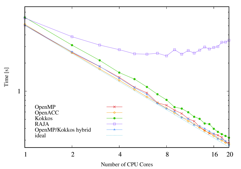
Figure 1: Log-log plot of the compute times per iteration as functions of the number of CPU cores. We compare the performance of Kokkos, RAJA, and OpenACC on the CPU to plain OpenMP. Moreover, the scaling curve of the hybrid code that uses OpenMP directive-based loop-parallelism on data stored in Kokkos views is shown. The codes were run on a 20-core Intel Xeon Gold 6148 2.4GHz (Skylake) CPU. The times shown were averaged over 10 runs.

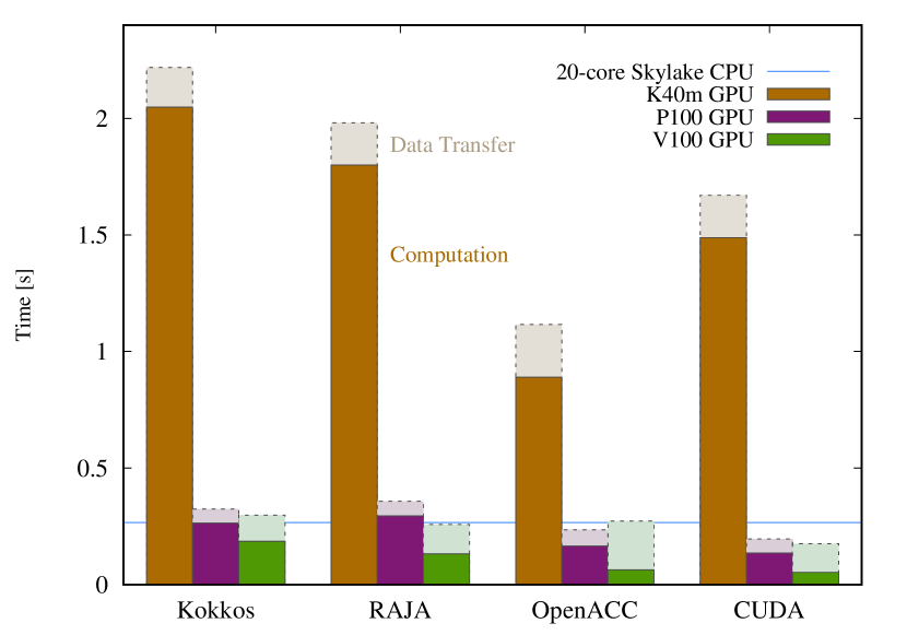
Figure 2: Plot of the times per iteration for various GPU models. We compare the performance of Kokkos, RAJA, and OpenACC to CUDA. In addition to the compute time the time necessary for one data transfer is shown. The codes were run on a NVIDIA K40m, a NVIDIA P100, and a NVIDIA V100 GPU. For direct comparison, a horizontal line indicates the best result obtained on the 20-core Intel Xeon Gold 6148 2.4GHz (Skylake) multicore CPU, cf. Fig. 1. The times shown for the GPUs were averaged over 200 runs.

4.3.1 CPU

On the CPU, the OpenACC implementation turns out to be the fastest and scales nearly ideally up to the full 20 Skylake cores with a speedup of about $19$. Following closely, the next-ranked CPU code is the plain OpenMP implementation which as well does show a near-ideal parallel scaling and speedup of about $18$. Overall, OpenMP is performing very similarly to OpenACC, it is only about $2.8$% slower on 20 cores. The Kokkos implementation, in comparison and averaged over the different core numbers under consideration, is about a factor of $1.21$ slower than the OpenACC code which we attribute to Kokkos-internal overhead. Obviously, the performance and also the scaling of the RAJA code is the worst in the present comparison, although the per-thread memory management was already improved (cf. Sec. 4.2.1). Presumably, this could be further optimized, however, this would require a considerable performance tuning effort which is exactly what one wants to avoid when choosing to build the implementation based on a performance portability framework. The hybrid implementation which uses plain OpenMP directives in combination with Kokkos views shows virtually identical performance as the plain OpenMP implementation, with a parallel speedup of $19.18$ on 20 cores. Hence, it is possible to optimize certain critical parts of a code in situations when the overhead from the Kokkos parallel execution is not acceptable.

4.3.2 GPU

Turning towards the GPUs, in addition to the compute time, we also have to consider the time for data transfers between the host and the device. In a full-fledged MPI-parallel PIC code, the operation on the particle data is embarrassingly parallel and only needs synchronization when particles are redistributed between processes due to particle sorting for reasons of data locality. Other occasions for the exchange of particle data between host and device are the initial setup or regular checkpointing. The frequency of such data transfers depends on the characteristics of a particular setup. Only the field data needs to be synchronized in each step, however, that data is almost negligibly small compared to the particle data. For our study, we therefore measure separately the compute time and the time needed for the data transfer, where we synchronized the data between host and device in each time step. The total time in a realistic scenario will usually be close to the pure compute time due to infrequent data transfers.

What concerns the data transfer time, it is important to first recall that the three GPU models under consideration use different interconnects. The P100 is connected via the NVLink communication bus with a transfer rate of 20 gigatransfers (GT) per second, while the K40m and the V100 use a PCIe 3.0 bus with a transfer rate of 8 GT/s. Therefore, the transfer times are roughly 2 times smaller with NVLink, as can be clearly seen from the plot. The compute and transfer times shown in Fig. 2 were determined using the NVIDIA nvprof profiler.

We now compare the compute time for the various implementations on the three GPU models. On the oldest GPU hardware, the K40m, the rank order is given by OpenACC, CUDA, RAJA, and Kokkos. CUDA is about $67$% slower than OpenACC. The RAJA runs take a factor of $2.02$ and the Kokkos runs take a factor of $2.30$ longer than the times measured for OpenACC. This order changes on the more recent hardware.

On the P100 GPU, the CUDA code is the fastest, followed by OpenACC ($1.23$), Kokkos ($1.95$), and RAJA, the latter being slower than CUDA by a factor of $2.18$.

On the V100 GPU, again CUDA delivers the fastest result, followed by OpenACC ($1.20$), RAJA ($2.51$), and finally Kokkos which is a factor of $3.53$ slower than CUDA. Note that in the OpenACC case, in particular, the transfer time is larger on the V100 (PCIe) than on the P100 (NVLink), which makes the OpenACC code overall run the fastest on the P100 GPU. Moreover, the compute time is by far the smallest on the V100 GPU for the CUDA implementation, where the data transfer takes about a factor of $2.3$ longer than the computation. In comparison to the best result from the 20-core Skylake CPU, the computation is significantly faster on the V100 in all cases.

The fact that the CUDA code becomes relatively faster when going to more recent GPUs is caused by an implementation detail. Atomic updates have received significantly improved hardware support with recent GPUs. Our CUDA implementation uses atomic additions on a global array to perform the reductions, whereas our OpenACC implementation uses atomic updates on per-gang private array copies followed by a final reduction across the gangs, reducing the concurrent accesses compared to the CUDA approach and therefore showing relatively better performance on the older K40m GPU. The OpenACC per-gang solution was chosen because it demonstrated much better performance on the multicore CPU compared to a solution with a single global array, while showing rather similar performance on the GPUs.

5 Summary

This paper presents a performance and usability assessment of two major performance portability frameworks, Kokkos and RAJA, which are considered for the future development of a high-performance C++ implementation of a particle-in-cell approach to solve the Vlasov–Maxwell equations. We focus on the node-local part of the computation, comparing generic implementations based on Kokkos, RAJA, and OpenACC, to CPU- and GPU-specific implementations based on OpenMP and CUDA, respectively.

5.1 Usability assessment

Considering programmability and usability, Kokkos and RAJA offer rather similar concepts and levels of abstraction. Both frameworks provide generic building blocks for parallel programming, targeting CPU and accelerator platforms. Code specialization to a specific processor is done at compile time based on C++ template meta programming, and is thus hidden from the user. Regarding the features necessary for our PIC application such as vector reductions and scratch memory, Kokkos offers all of them whereas for RAJA some additional implementation work was needed.

Kokkos provides useful default values for the majority of relevant template parameters. If not specified otherwise, the code is compiled for the “fastest” architecture available, as defined by the ordering CUDA, OpenMP, pthreads, and serial. With the default parameters, the execution space (CPU or GPU) of a parallel section will automatically match the memory space (host memory or device memory) which significantly facilitates implementation and simplifies the code. Moreover, with Kokkos we managed avoiding architecture-specific preprocessor macros in the code. The Kokkos project is very well documented and the developers are supportive on GitHub, according to our experience. As a plus, a simple architecture-specification string set by the user in the Kokkos Makefile automatically enables the correct set of hardware-specific optimization flags for the compiler.

RAJA does not implement such architectural default values for the template parameters. Hence, the user has to specify the architecture-specific parameters explicitly, e.g. by employing preprocessor macros. RAJA required us to have multiple of such branches in the code for CPU and GPU compilation. While this adds some fine-grained control options, the underlying paradigm of writing a single source code for multiple architectures gets somewhat compromised.

It should be noted that both the Kokkos-GPU and RAJA-GPU codes for our PIC application were obtained “for free” in the sense that all development started out on multi-core CPUs and no GPU-specific code was ever written (except for some preprocessor branches to set template parameters in the case of RAJA), thereby confirming the idea of portability at good performance.

5.2 Performance assessment

In total, seven C++ versions of the PIC routine were developed, namely a sequential one, and parallel codes using OpenMP, OpenACC, CUDA, Kokkos, hybrid OpenMP/Kokkos, and RAJA. The performance was measured on a Skylake multicore CPU and on three NVIDIA GPUs from different hardware generations. Only limited effort was spent on optimizing each individual implementation.

On the CPU, Kokkos shows acceptable overhead compared to plain OpenMP of about 14% and scales nearly as well as plain OpenMP. Moreover, we have also demonstrated that the overhead of the Kokkos framework over a pure OpenMP implementation is not linked to the use of Kokkos views for data management. Therefore, it is possible to mitigate the performance penalty of the Kokkos framework by manually optimizing critical kernels. The results we have obtained with RAJA appear a bit inferior on the CPU since the parallel scalability is hampered by a false sharing issue that could only partially be solved. On the other hand, the performance on the GPU is comparable or even slightly better than the one of Kokkos across different GPU hardware generations. On state-of-the-art GPUs, CUDA turns out to be the fastest choice, followed by OpenACC, Kokkos and RAJA. Overall, OpenACC is very competitive on both, the CPU and the GPU, and should be kept in mind as an option for performance portability, especially with improved compiler support that is to be expected in the near future (GCC and LLVM, in addition to PGI).

In summary, both Kokkos and RAJA seem mature, usable for production codes, and keep their promise to provide performance portability across different hardware architectures.

Appendix A Numerical model

This section gives a more detailed description of the equations implemented in our case study. The basis for particle-in-cell methods are the characteristic equations associated to (1) are given by

$$\frac{\text{d}\textbf{X}}{\text{d}t}=\textbf{V},\quad\frac{\text{d}\textbf{V}}{\text{d}t}=\left(\textbf{E}(\textbf{X},t)+\textbf{V}\times\textbf{B}(\textbf{X},t)\right),$$ (4)

along which the value of the distribution function remains constant over time. Particle methods represent the distribution function by a number $N_{p}$ of macro-particles that evolve according to the characteristic equations. The macro-particles are characterized by their position in phase space and a weight, that is particle $p$ is represented by $(\textbf{x}_{p},\textbf{v}_{p},w_{p})$. The particle position and velocity are dynamic variables following the characteristic equations (4) and the weights are constant in time (note that time-dependent weights are also possible in advanced setups but are not discussed here). In order to compute the velocity moments of the distribution function needed to solve Maxwell’s equations, a representation of the distribution function is necessary. This is usually given by

$$f_{s}(\textbf{x},\textbf{v},t)=\sum_{p=1}^{N_{p_{s}}}w_{p}S(\textbf{x}-\textbf{x}_{p})\delta(\textbf{v}-\textbf{v}_{p}),$$ (5)

where $S$ can either be a $\delta$ distribution or a smoothing kernel. Finally, the fields are represented on a grid and Maxwell’s equations are solved by finite elements or finite differences. Multiple discretization schemes have been discussed in the literature which have similar building blocks based on solutions of the field equations and loops over the particles with field evaluations for the particle push and current or charge depositions to assemble the source terms for the Maxwell’s equations. Since usually the number of particles is much larger than the number of degrees of freedom in the description of the fields, the computational complexity is dominated by the particle loop.

The motivation of our work is an efficient and portable implementation of the scheme proposed in Ref. [18] for the Vlasov–Maxwell equations. The scheme uses compatible spline finite elements as proposed by Buffa et al. [20] for the fields and a Klimontovic distribution for the particle distribution (i.e. $S=\delta$). Basis functions of different order are used to represent the magnetic and the electric field, respectively. Let us denote by $\Lambda^{1,k}_{i}$ the basis functions for component $k$, $k=1,2,3$, of the electric field associated with the grid point $i$, $i=1,\ldots,N_{g}$. In the same way, we denote by $\Lambda^{2,k}_{i}$ the basis functions for component $k$, $k=1,2,3$, of the magnetic field associated with grid point $i$, $i=1,\ldots,N_{g}$. Then, the semi-discretized fields are represented as

$$\tilde{}\textbf{E}_{k}(\textbf{x},t)=\sum_{i=1}^{N_{g}}e_{k,i}(t)\Lambda^{1,k}_{i}(\textbf{x}),\quad\tilde{}\textbf{B}_{k}(\textbf{x},t)=\sum_{i=1}^{N_{g}}b_{k,i}(t)\Lambda^{2,k}_{i}(\textbf{x}).$$ (6)

with $\textbf{e}_{k}=\left(e_{k,1},\ldots,e_{k,N_{g}}\right)^{\top}$ and $\textbf{b}_{k}=\left(b_{k,1},\ldots,b_{k,N_{g}}\right)^{\top}$ being the dynamic variables. Given a certain degree $p$, the basis functions are constructed in the following way:

• $\Lambda^{1,k}$ is constructed as a tensor product of splines of degree $p-1$ in $x_{k}$ and of degree $p$ along the other two dimensions,

• $\Lambda^{2,k}$ is constructed as a tensor product of splines of degree $p$ in $x_{k}$ and of degree $p-1$ along the other two dimensions.

Furthermore, equation (2a) is solved in weak form and (2b) is solved in strong form. Inserting the representation of the fields and particles into the equations yields the following semi-discrete equations of motion

$$\frac{\text{d}\textbf{X}}{\text{d}t} =\textbf{V},$$ (7a)

$$\frac{\text{d}\textbf{V}_{1}}{\text{d}t} =\frac{q}{m}\left(\mathbb{\Lambda}^{1,1}(\textbf{X})\textbf{e}_{1}+\textbf{V}_{2}\mathbb{M}_{q}\mathbb{\Lambda}^{2,3}(\textbf{X})\textbf{b}_{3}-\textbf{V}_{3}\mathbb{M}_{q}\mathbb{\Lambda}^{2,2}(\textbf{X})\textbf{b}_{2}\right)$$

$$\frac{\text{d}\textbf{V}_{2}}{\text{d}t} =\frac{q}{m}\left(\mathbb{\Lambda}^{1,2}(\textbf{X})\textbf{e}_{2}+\textbf{V}_{3}\mathbb{M}_{q}\mathbb{\Lambda}^{2,1}(\textbf{X})\textbf{b}_{1}-\textbf{V}_{1}\mathbb{M}_{q}\mathbb{\Lambda}^{2,3}(\textbf{X})\textbf{b}_{3}\right),$$ (7b)

$$\frac{\text{d}\textbf{V}_{3}}{\text{d}t} =\frac{q}{m}\left(\mathbb{\Lambda}^{1,3}(\textbf{X})\textbf{e}_{3}+\textbf{V}_{1}\mathbb{M}_{q}\mathbb{\Lambda}^{2,2}(\textbf{X})\textbf{b}_{2}-\textbf{V}_{2}\mathbb{M}_{q}\mathbb{\Lambda}^{2,1}(\textbf{X})\textbf{b}_{1}\right),$$ (7c)

$$\frac{\text{d}\textbf{e}}{\text{d}t} =\mathbb{M}_{1}^{-1}\left(\mathbb{C}^{\top}\mathbb{M}_{2}\textbf{b}(t)-\mathbb{\Lambda}^{1}(\textbf{X})^{\top}\mathbb{M}_{q}\textbf{V}\right),$$ (7d)

$$\frac{\text{d}\textbf{b}}{\text{d}t} =-\mathbb{C}\textbf{e}(t).$$ (7e)

The dynamic variables are given by $(\textbf{X},\textbf{V},\textbf{e},\textbf{b})$, where $\textbf{X}=\left(\textbf{x}_{1}^{\top},\ldots,\textbf{x}_{N_{p}}^{\top}\right)^{\top}$ and $\textbf{V}=\left(\textbf{v}_{1}^{\top},\ldots,\textbf{v}_{N_{p}}^{\top}\right)^{\top}$, $\textbf{e}=(\textbf{e}_{1}^{\top},\textbf{e}_{2}^{\top},\textbf{e}_{3}^{\top})^{\top}$, $\textbf{b}=(\textbf{b}_{1}^{\top},\textbf{b}_{2}^{\top},\textbf{b}_{3}^{\top})^{\top}$. Furthermore, $\mathbb{C}$ represents the discrete curl matrix, $\mathbb{M}_{j}$ the finite element mass matrix for basis $j=1,2$, and $\mathbb{M}_{q}$ is a diagonal matrix with the product of the particle weight and charge on the diagonals. The matrix $\mathbb{\Lambda}^{j}=(\mathbb{\Lambda}^{j,1},\mathbb{\Lambda}^{j,2},\mathbb{\Lambda}^{j,3})$ is a $N_{p}\times(3N_{g})$ matrix with entries $(\mathbb{\Lambda}^{j,k})_{p,i}=\Lambda^{j,k}_{i}(\textbf{x}_{p})$.

These equations can either be solved by some implicit time-stepping scheme or by a splitting of the equations into several subsystem that are chosen in such a way that the substeps can be solved explicitly. Such an explicit time stepping scheme, called Hamiltonian splitting, has been proposed in Ref. [18]. For this study, we implement only one of the building blocks of the complete scheme that, however, contains the main features of the overall schemes. The building blocks solves the following part of the equations

$$\frac{\text{d}\textbf{X}_{1}}{\text{d}t} =\textbf{V}_{1},$$ (7ha)

$$\frac{\text{d}\textbf{V}_{2}}{\text{d}t} =-\frac{q}{m}\textbf{V}_{1}\mathbb{M}_{q}\mathbb{\Lambda}^{2,3}(\textbf{X})\textbf{b}_{3},$$ (7hb)

$$\frac{\text{d}\textbf{V}_{3}}{\text{d}t} =\frac{q}{m}\textbf{V}_{1}\mathbb{M}_{q}\mathbb{\Lambda}^{2,2}(\textbf{X})\textbf{b}_{2},$$ (7hc)

$$\mathbb{M}_{1,1}\frac{\text{d}\textbf{e}_{1}}{\text{d}t} =-\mathbb{\Lambda}^{1,1}(\textbf{X})^{\top}\mathbb{M}_{q}\textbf{V}_{1},$$ (7hd)

by explicit integration over time as

$$x_{1,p}(t_{m+1}) =x_{1,p}(t_{m})+\Delta tv_{1,p},$$ (7ia)

$$v_{2,p}(t_{m+1}) =v_{2,p}(t_{m})-\frac{q}{m}\sum_{i=1}^{N_{g}}b_{3,i}(t_{m})\int_{t_{m}}^{t_{m+1}}\Lambda^{2,3}(\textbf{x}_{p}(\tau))v_{1,p}(t_{m})\text{d}\tau,$$ (7ib)

$$v_{3,p}(t_{m+1}) =v_{3,p}(t_{m})+\frac{q}{m}\sum_{i=1}^{N_{g}}b_{2,i}(t_{m})\int_{t_{m}}^{t_{m+1}}\Lambda^{2,2}(\textbf{x}_{p}(\tau))v_{1,p}(t_{m})\text{d}\tau,$$ (7ic)

$$\mathbb{M}_{1,1}\textbf{e}_{1}(t_{m+1}) =\mathbb{M}_{1,1}\textbf{e}_{1}(t_{m})-q\sum_{p=1}^{N_{p}}w_{p}\int_{t_{m}}^{t_{m+1}}\mathbb{\Lambda}^{1,1}(\textbf{x}_{p}(\tau))v_{1,p}(t_{m})\text{d}\tau.$$ (7id)

where $\textbf{x}_{p}(\tau)=\left(x_{1,p}(t_{m})+\tau v_{1,p}(t_{m}),x_{2,p}(t_{m}),x_{3,p}(t_{m})\right)^{\top}$. The computationally most expensive part is to evaluate the integrals over the basis functions. If the velocity $v_{1,p}(t_{m})$ is nonzero, we can transform the integral from $\tau$ to $\sigma=x_{1,p}(t_{m})+\tau v_{1,p}(t_{m})$. Then equation (7ib) reads

$$v_{2,p}(t_{m+1})=v_{2,p}(t_{m})-\frac{q}{m}\sum_{i=1}^{N_{g}}b_{3,i}(t_{m})\int_{x_{1,p}(t_{m})}^{x_{1,p}(t_{m+1})}\Lambda^{2,3}(\sigma,x_{2,p}(t_{m}),x_{3,p}(t_{m}))\text{d}\sigma.$$ (7j)

The other integrals can be transformed in a similar way. Next, we apply the tensor product of one-variate splines $N^{q}(x)$ of degree $q=p$ and $q=p-1$ as proposed before. Then, the update of the particle velocities and the contribution of particle $p$ to component $i$ of the integrated current $j_{i}$ reads

$$v_{2,p}(t_{m+1}) =v_{2,p}(t_{m})-\frac{q}{m}\sum_{i=1}^{N_{g}}b_{3,i}(t_{m})\int_{x_{1,p}(t_{m})}^{x_{1,p}(t_{m+1})}N_{i_{1}}^{p-1}(\sigma)\text{d}\sigma N_{i_{1}}^{p-1}(x_{2,p}(t_{m}))N_{i_{3}}^{p}(x_{3,p}(t_{m}))$$ (7ka)

$$v_{3,p}(t_{m+1}) =v_{3,p}(t_{m})+\frac{q}{m}\sum_{i=1}^{N_{g}}b_{2,i}(t_{m})\int_{x_{1,p}(t_{m})}^{x_{1,p}(t_{m+1})}N_{i_{1}}^{p-1}(\sigma)\text{d}\sigma N_{i_{1}}^{p}(x_{2,p}(t_{m}))N_{i_{3}}^{p-1}(x_{3,p}(t_{m})),$$ (7kb)

$$j_{i} =j_{i}+qw_{p}\int_{x_{1,p}(t_{m})}^{x_{1,p}(t_{m+1})}N_{i_{1}}^{p-1}(\sigma)\text{d}\sigma N_{i_{1}}^{p}(x_{2,p}(t_{m}))N_{i_{3}}^{p}(x_{3,p}(t_{m})),$$ (7kc)

where we decompose the unique index $i$ for the basis functions into a three dimensional index $(i_{1},i_{2},i_{3})$ reflecting the tensor product structure of the basis. Since the basis functions have compact support, we identify first in which grid cell the particle is located and then we evaluate the $q+1$ basis functions (of degree $q$) with support on this cell. To evaluate the splines, we use their representation in piecewise polynomial form (pp-form) using Horner’s algorithm at the particle position (normalized to the grid cell). For the evaluation of the integral, we evaluate the primitive basis function at the new and old position. This can either be implemented using numerical quadrature or based on the primitive function of $N^{p-1}$. We choose the latter approach and denoting the primitive of $N^{p-1}$ by $\mathcal{N}$, we get

$$\int_{x_{1,p}(t_{m})}^{x_{1,p}(t_{m+1})}N_{i_{1}}^{p-1}(\sigma)\text{d}\sigma=\mathcal{N}_{i_{1}}(x_{1,p}(t_{m+1}))-\mathcal{N}_{i_{1}}(x_{1,p}(t_{m})).$$ (7l)

We note that the support of a spline of degree $p-1$ is $p$ cells while the support of this integral is variable depending on how large the difference $x_{1,p}(t_{m+1})-x_{1,p}(t_{m})$ between the old and new particle position is. We note that this results in a variable loop length that makes it harder to design data structures for efficient and vectorized current deposition of this particular scheme.

Appendix B Color-coded implementation comparison of the PIC routine

The source code shown in listing 4 contains the key features necessary to implement the PIC routine for each parallel programming model under investigation. In particular the color coding is as follows: Black for common code, blue for OpenMP, brown for OpenACC, red for Kokkos, green for RAJA, purple for CUDA, and orange for hybrid OpenMP/Kokkos. Note that the listing presents a concatenation from the different source code parts for illustration purposes.

Listing 4: Color-coded key implementation features of the PIC routine for direct comparison.

⬇

// Class particle group: Basic data structure saving

// the information on all particles of one species

class particle_group_base_Kokkos {

KOKKOS_FUNCTION particle_group_base_Kokkos(char*, long, bool);

// common particle weight

double common_weight;

ViewScalarDoubleType view_common_weight;

ViewScalarDoubleType::HostMirror view_common_weight_host;

// array storing position in phase space and weight for each of n_particles

double** particle_array;

ViewVector2DType view_particle_array;

ViewVector2DUnmanagedType view_particle_array_unmanaged;

ViewVector2DType::HostMirror view_particle_array_host;

// information about the species ( mass and charge )

double m; //mass of a single particle

ViewScalarDoubleType view_m;

ViewScalarDoubleUnmanagedType view_m_unmanaged;

ViewScalarDoubleType::HostMirror view_m_host;

//charge

double q; //charge of a single particle

ViewScalarDoubleType view_q;

ViewScalarDoubleUnmanagedType view_q_unmanaged;

ViewScalarDoubleType::HostMirror view_q_host;

// number of particles in the particle group

long n_particles;

ViewScalarLongType view_n_particles;

ViewScalarLongUnmanagedType view_n_particles_unmanaged;

ViewScalarLongType::HostMirror view_n_particles_host;

// Next the accessor functions are defined

{ ... }

}

class particle_group_base_RAJA {

particle_group_base_RAJA(string, long, bool);

// common particle weight

double common_weight;

// array storing position in phase space and weight for each of n_particles

double** particle_array;

double* d_particle_array;

RajaVector2DType raja_particle_array;

// information about the species ( mass and charge )

double m; //mass of a single particle

double *d_m;

RajaVector1DType raja_m;

double q; //charge of a single particle

double *d_q;

RajaVector1DType raja_q;

// number of particles in the particle group

long n_particles;

long *d_n_particles;

RajaVector1DLongType raja_n_particles;

// Next the accessor functions are defined

{ ... }

}

class particle_group_base_cuda {

particle_group_base_cuda(string, long, bool);

// common particle weight

double common_weight;

// array storing position in phase space and weight for each of n_particles

double** particle_array;

double* d_particle_array;

// information about the species ( mass and charge )

double m; //mass of a single particle

double *d_m;

double q; //charge of a single particle

double *d_q;

// number of particles in the particle group

long n_particles;

long *d_n_particles;

// Next the accessor functions are defined

{ ... }

}

void hamiltonian_splitting::pic_routine(double dt,

int n_threads, int n_teams

int n_threads

int n_threads) {

int total_num_threads = omp_get_max_threads();

//OpenMP: initialisation of the reduction array

double j_dofs[total_num_threads][this->part_mesh_coupling.n_dofs];

for(int i=0; i<total_num_threads; i++) {

for(int j=0; j<this->part_mesh_coupling.n_dofs; j++) {

j_dofs[i][j] = 0.0;

}

}

//Kokkos: initialisation of the reduction array

for(long i=0; i<this->view_j_dofs_local_host.size(); i++) {

this->view_j_dofs_local_host(i) = 0.0;

}

Kokkos::deep_copy(this->view_j_dofs_local, this->view_j_dof_local_host);

int total_num_threads = std::max(atoi(std::getenv("OMP_NUM_THREADS")), 1);

//RAJA: initialisation of the reduction array

#if defined(RAJA_ENABLE_CUDA) && defined(I_USE_CUDA)

RAJA::forall<RAJA::cuda_exec<256>>(RAJA::RangeSegment(0, this->part_mesh_coupling.n_dofs),

[*this] RAJA_DEVICE (int i) {

if(i<this->part_mesh_coupling.raja_n_dofs(0)) {

this->raja_j_dofs_local(i) = 0.0;

}

});

#else

RAJA::forall<RAJA::omp_parallel_for_exec>(RAJA::RangeSegment(0, this->part_mesh_coupling.n_dofs),

[this] (int i) {

if(i<part_mesh_coupling.raja_n_dofs(0)) {

raja_j_dofs_local(i) = 0.0;

}

});

#endif

int M_blocks = (this->particle_group.group[0].n_particles + n_threads-1)/n_threads; //#of blocks

//CUDA: no reduction array, atomic operations are used instead

int total_num_threads = omp_get_max_threads();

//Hybrid: initialisation of the reduction array

double j_dofs[total_num_threads][this->part_mesh_coupling.view_n_dofs_host(0)];

for(int i=0; i<total_num_threads; i++) {

for(int j=0; j<this->part_mesh_coupling.view_n_dofs_host(0); j++) {

j_dofs[i][j] = 0.0;

}

}

//Hybrid: set all unmanaged views

this->view_i_weight_unmanaged = this->view_i_weight;

{...}

int total_num_gangs = input_n_gangs();

int total_num_vectors = input_n_vectors();

//OpenACC: initialisation of the reduction array

double **j_dofs = (double**)malloc(total_num_gangs * sizeof(double *));

for(int i=0; i<total_num_gangs; i++) {

j_dofs[i] = (double*)malloc(this->part_mesh_coupling.n_dofs * sizeof(double));

for(int j=0; j<this->part_mesh_coupling.n_dofs; j++) {

j_dofs[i][j] = 0.0;

}

}

#pragma omp parallel

{

//OpenMP: initialisation of the local variables

{...}

for(long i_sp = 0; i_sp<this->particle_group.n_species; i_sp++) {

//OpenMP: get thread ID, set qoverm

{...}

#pragma omp for

for(long i_part=0; i_part<this->particle_group.group[i_sp].n_particles; i_part++) {

{operator_openmp}

}

#pragma omp for

for(int i=0; i<this->part_mesh_coupling.n_dofs; i++) {

for(int thread=1; thread<total_num_threads; thread++) {

j_dofs[0][i] += j_dofs[thread][i];

}

}

}

}

//Kokkos: set dt

{...}

for(long i_sp = 0; i_sp<this->particle_group.view_n_species_host(0); i_sp++) {

//Kokkos: set view_i_sp and shared_size=n_shared*sizeof(double)

{...}

//Kokkos: set parallel policy

auto policy = Kokkos::TeamPolicy<pic_routine, ExecSpace>((this->particle_group.view_group_host(i_sp).n_particles + n_threads-1)/n_threads, n_threads)

.set_scratch_size(1,Kokkos::PerThread(shared_size));

//Kokkos: parallel computation

Kokkos::parallel_for(policy, *this);

}

//RAJA: set dt

{...}

for(long i_sp = 0; i_sp<this->particle_group.n_species; i_sp++) {

//RAJA: set view_i_sp and shared_size

#if defined(RAJA_ENABLE_CUDA) && defined(I_USE_CUDA)

//RAJA: GPU parallel computation

RAJA::forall<RAJA::cuda_exec<256>>(RAJA::RangeSegment(0, this->particle_group.group[0].n_particles),

[=,*this] RAJA_DEVICE (int i_part) {

{operator_RAJA_GPU} //RAJA GPU: uses atomics instead of reduction

});

#else

//RAJA CPU: raja_private_raja_array is our solution to false-sharing

//It is an array of struct such that each thread gets contiguous memory to use as scratch

//RAJA: set parallel policy

using fdPolicy = RAJA::KernelPolicy< RAJA::statement::For< 0, RAJA::omp_parallel_for_exec, RAJA::statement::Lambda<0> > >;

//RAJA CPU: initialisation of the handmade reduction 2D array

RAJA::kernel<fdPolicy>(RAJA::make_tuple(RAJA::RangeSegment(0, total_num_threads)),

[&,this] (int i_part) {

for(int i=0; i<this->part_mesh_coupling.n_dofs; i++)

this->raja_private_raja_array(i_part).raja_handmade_reduce(i) = 0.0;

});

//RAJA: CPU parallel computation

RAJA::kernel<fdPolicy>(RAJA::make_tuple(RAJA::RangeSegment(0, this->particle_group.group[0].n_particles)),

[&,this] (int i_part) {

{operator_RAJA_CPU}

});

//RAJA: CPU handmade reduction

RAJA::kernel<fdPolicy>(RAJA::make_tuple(RAJA::RangeSegment(0, this->part_mesh_coupling.n_dofs)),

[&,this] (int i_part) {

for(int i=0; i<total_num_threads; i++)

this->d_j_dofs_local[i_part] += this->raja_private_raja_array(i).raja_handmade_reduce(i_part);

});

#endif

}

//CUDA: parallel computation

operator_cuda<<<M_blocks,n_threads>>>(0.05, 0, this->d_particle_group, this->d_part_mesh_coupling,

this->d_control_vari, this->i_weight, this->d_bfield_dofs, this->d_j_dofs_local, this->d_Lx);

#pragma omp parallel

{

//Hybrid: initialisation of the local variables

{...}

for(long i_sp = 0; i_sp<this->particle_group.view_n_species_unmanaged(0); i_sp++) {

//Hybrid: get thread ID, set qoverm

{...}

#pragma omp for

for(long i_part=0; i_part<this->particle_group.view_group_unmanaged( this->view_i_species_unmanaged(0) ).view_n_particles_unmanaged(0); i_part++) {

{operator_hybrid}

}

#pragma omp for

for(int i=0; i<this->part_mesh_coupling.view_n_dofs_unmanaged(0); i++) {

for(int thread=1; thread<total_num_threads; thread++) {

j_dofs[0][i] += j_dofs[thread][i];

}

}

}

}

#pragma acc data

copy(j_dofs[0:total_num_gangs][0:this->part_mesh_coupling.n_dofs])

copyin(this[0:1],

this->part_mesh_coupling,

this->part_mesh_coupling.domain[0:3][0:2],

this->part_mesh_coupling.delta_x[0:3],

this->part_mesh_coupling.rdelta_x[0:3],

this->part_mesh_coupling.spline_0,

this->part_mesh_coupling.spline_0.d_poly_coeffs[0:(spline_0_degree+1)*(spline_0_degree+1)],

this->part_mesh_coupling.spline_0.d_poly_coeffs_fpa[0:(spline_0_degree+2)*(spline_0_degree+1)],

this->part_mesh_coupling.spline_1,

this->part_mesh_coupling.spline_1.d_poly_coeffs[0:(spline_1_degree+1)*(spline_1_degree+1)],

this->part_mesh_coupling.spline_1.d_poly_coeffs_fpa[0:(spline_1_degree+2)*(spline_1_degree+1)],

this->part_mesh_coupling.n_grid[0:3],

this->part_mesh_coupling,

this->Lx[0:3],

this->bfield_dofs[0:this->part_mesh_coupling.n_dofs*3],

this->particle_group,

this->particle_group.group[0:this->particle_group.n_species],

this->particle_group.group[0].sp),

copy( this->particle_group.group[0].particle_array[0:7][0:this->particle_group.group[0].n_particles])

{

#pragma acc parallel num_gangs(total_num_gangs) vector_length(total_num_vectors)

{

//OpenACC: initialisation of the per-gang reduction j_dofs, local variables and get gang ID

int this_gang = __pgi_gangidx();

{...}

for(long i_sp = 0; i_sp<this->particle_group.n_species; i_sp++) {

//OpenACC: set qoverm

{...}

#pragma acc loop

for(long i_part=0; i_part<this->particle_group.group[i_sp].n_particles; i_part++) {

{operator_openacc}

}

}

}

}

//OpenMP: copying the reduction’s result

for(int i=0; i<this->part_mesh_coupling.n_dofs; i++) {

this->j_dofs_local[i] = j_dofs[0][i];

}

//Hybrid: copying the reduction’s result

for(int i=0; i<this->part_mesh_coupling.view_n_dofs(0); i++) {

this->view_j_dofs_local(i) = j_dofs[0][i];

}

//OpenACC: second reduction on the gang results

for(int i=0; i<total_num_gangs; i++) {

for(int j=0; j<this->part_mesh_coupling.n_dofs; j++) {

this->j_dofs_local[j] += j_dofs[i][j];

}

}

//OpenACC: free memory

for(int i=0; i<total_num_gangs; i++)

free(j_dofs[i]);

free(j_dofs);

}

operator_openmp {

KOKKOS_FUNCTION void hamiltonian_splitting::operator() (const pic_routine&, const Kokkos::TeamPolicy<>::member_type & team_member) const {

operator_RAJA_GPU {

operator_RAJA_CPU {

__global__ void operator_cuda(double dt, int i_sp, particles *d_particle_group, particle_mesh_coupling *d_part_mesh_coupling, control_variate *d_control_vari, long i_weight, double *d_bfield_dofs, double *d_j_dofs, double *d_Lx) {

operator_hybrid {

operator_openacc {

//Kokkos: thread access to special scatter view, used for vector reduction

ViewScatterAccessType scatter_access = this->scatter_view.access();

//Kokkos: initialise scratch variables

ViewVector3ScratchType view_x_old(team_member.thread_scratch(1));

{...}

//RAJA GPU: initialisation of the local variables BUT WITH FIXED SIZE

//The size is given by the number of dimensions (3) by the support of the spline (4 here for cubic splines, but should be templated for varying order).

double d_spline_0[4*3];

{...}

//CUDA: initialisation of the local variables (and qoverm) BUT WITH FIXED SIZE

double d_spline_0[4*3]; // Size as for RAJA.

{...}

//OpenACC: initialisation of the local variables (and qoverm) BUT WITH FIXED SIZE

double d_spline_0[4*3]; // Size as for RAJA.

{...}

//Read out particle position and velocity

{...}

//Then update particle position: X_new(0) = X_old(0) + dt * V(0)

x_new[0] = x_old[0] + dt * vi[0];

x_new[1] = x_old[1];

x_new[2] = x_old[2];

//Get charge for accumulation of j

{...}

this->part_mesh_coupling.add_current_update_v_primitive_component1_spline_3d_feec_util (res[this_thread], x_old, x_new[0], wi[0], qoverm,

this->bfield_dofs, vi, &util_arrays);

this->part_mesh_coupling.view_add_current_update_v_primitive_component1_spline_3d_feec_scratch (team_member,

view_x_old, view_x_new(0), view_wi(0), qoverm,

this->view_bfield_dofs, view_vi, &(this->scatter_view));

this->part_mesh_coupling.raja_add_current_update_v_primitive_component1_spline_3d_feec_util (raja_x_old, raja_x_new(0), raja_wi(0), qoverm,

this->raja_bfield_dofs, raja_vi, this->d_j_dofs_local, &util_raja); //GPU

this->part_mesh_coupling.raja_add_current_update_v_primitive_component1_spline_3d_feec_util_pool_thread<0>

(THREAD, this->raja_private_raja_array(THREAD).raja_x_old,

this->raja_private_raja_array(THREAD).raja_x_new(0), this->raja_private_raja_array(THREAD).raja_wi(0),

qoverm, this->raja_bfield_dofs, this->raja_private_raja_array(THREAD).raja_vi,

this->raja_private_raja_array(THREAD).raja_handmade_reduce, this->raja_private_raja_array(THREAD)); //CPU

d_part_mesh_coupling->cuda_add_current_update_v_primitive_component1_spline_3d_feec_util (x_old, x_new[0], wi[0], qoverm,

d_bfield_dofs, vi, d_j_dofs, &util_cuda);

this->part_mesh_coupling.add_current_update_v_primitive_component1_spline_3d_feec_util_from_view (j_dofs[this_thread], x_old, x_new[0], wi[0], qoverm,

&this->view_bfield_dofs_unmanaged, vi, &util_arrays);

this->part_mesh_coupling.add_current_update_v_primitive_component1_spline_3d_feec_util_openacc (j_dofs[this_gang], x_old, x_new[0], wi[0], qoverm,

this->bfield_dofs, vi, &util_openacc);

x_new[0] = fmod(x_new[0] + this->Lx[0], this->Lx[0]);

this->particle_group.group[i_sp].set_x(i_part, x_new);

this->particle_group.group[i_sp].set_v(i_part, vi);

}

void particle_mesh_coupling::add_current_update_v_primitive_component1_spline_3d_feec_util (double *j_dofs,

double *position_old, double position_new, double marker_charge, double qoverm,

double *bfield_dofs,

ViewVector1DUnmanagedType *view_bfield_dofs_unmanaged, //instead of double *bfield_dofs

double *vi, struct private_arrays *util_arrays,

struct private_raja util_raja //GPU

struct private_raja * util_raja //CPU

struct private_cuda util_cuda

struct private_openacc util_openacc

) {

//Initialise local variables (and qoverm) BUT WITH FIXED SIZE

{...}

ViewScatterAccessType view_j_dofs_scatter_access = view_j_dofs_scatter->access();

// Identify the grid cell (box) where the particle is located and

// its normalized position (xi) within the box

{...}

// Similarly as above, we identify box and normalized position for the

// new position (along x(component) only)

{...}

// Extract box index along the direction component for the old position

{...}

// In the tensor product basis, the three 1D components are

// combined with each other in every possible combination

// Therefore, we start by computing the three 1D components

{...}

// Along x(0), we have to integrate over splines of degree degree-1

// We get a contribution to the current in all indices of

// splines that are nonzero in either boxnew or boxold

// In each box, degree basis function are nonzero

// This gives the following number of nonzero values of

// the total integral

{...}

// First we evaluate the primitive of the degree basis functions that are

// nonzero at the old and new particle positions respectively

// For this we use the pp coefficients of the primitive function

// of the splines and evaluate using Horner’s scheme

{...}

// Now, we glue everything together

// Note that the primitive function is equal to delta_x(component)

// in all intervals with index larger that the indices of the

// support of the basis function

{...}

// For the other two other directions, we need to evaluate the splines of

// degree p and (p-1) at the particle position

{...}

// We use the pp form and evaluate with Horner’s scheme

{...}

// Set index of first basis function that is nonzero at

// the particle position

// Set index of first basis function that is nonzero at

// the particle position for the dimension with integration

{...}

//optimisation : precomputations of the indices

{...}

// loop over all the basis functions that are nonzero at the

// particle position and update velocities and current

for(long k=0; k<this->spline_degree+1; k++) {

vtt2 = 0.0; vtt3 = 0.0;

for(long j=0; j<this->spline_degree+1; j++) {

// Save the 2D spline product to avoid recomputation in the inner loop

splinejk = util_arrays->spline_0[1][j] * util_arrays->spline_0[2][k] * marker_charge;

util_arrays->vt[0] = 0.0; util_arrays->vt[1] = 0.0;

for(long i=0; i<local_size; i++) {

// Compute 1D index of the basis function from the 3D tensor product index

index1d = util_arrays->startjk[k][j] + util_arrays->index_x[i];

// update the current

j_dofs[index1d] += util_arrays->j1d[i] * splinejk;

view_j_dofs_scatter_access(index1d) += view_j1d(i) * splinejk;

RAJA::atomic::atomicAdd<RAJA::atomic::cuda_atomic>(&(d_j_dofs_tmp[index1d]), util_raja->raja_j1d(i) * splinejk); //GPU

d_j_dofs_tmp(index1d) += util_raja.raja_j1d(i) * splinejk; //CPU

atomicAdd(&(d_j_dofs_tmp[index1d]), util_cuda->d_j1d(i) * splinejk);

j_dofs[index1d] += util_arrays->j1d[i] * splinejk;

#pragma acc atomic

j_dofs[index1d] += util_openacc->d_j1d[i] * splinejk;

// contributions for the velocities

util_arrays->vt[0] += bfield_dofs[start1+index1d] * util_arrays->j1d[i];

util_arrays->vt[1] += bfield_dofs[start2+index1d] * util_arrays->j1d[i];

}

if(j>0) {

vtt2 += util_arrays->vt[0]*util_arrays->spline_1[1][j-1];

}

vtt3 -= util_arrays->vt[1]*util_arrays->spline_0[1][j];

}

// update the velocities

vi[1] -= qoverm*vtt2*util_arrays->spline_0[2][k];

if(k>0) {

vi[2] -= qoverm*vtt3*util_arrays->spline_1[2][k-1];

}

}

}

References

- [1] Strohmaier E, Dongarra J, Simon H, Meuer M. Top 500. The List.. https://www.top500.org; 2019. Accessed: 2019/03/18.
- [2] Forum TM. MPI: A Message Passing Interface. https://www.mpi-forum.org/docs/; 1993.
- [3] Wolfe M. Compilers and More: MPI+X. https://www.hpcwire.com/2014/07/16/compilers-mpix/; 2014. Accessed: 2019/03/21.
- [4] OpenMP Architecture Review Board . OpenMP Application Programming Interface. https://www.openmp.org/wp-content/uploads/OpenMP-API-Specification-5.0.pdf; 2018. Accessed: 2019/03/21.
- [5] OpenACC-Standard.org . The OpenACC Application Programming Interface Version 2.7. https://www.openacc.org/sites/default/files/inline-files/OpenACC.2.7.pdf; 2018. Accessed: 2019/03/21.
- [6] Khronos OpenCL Working Group . The OpenCL Specification Version 2.2. https://www.khronos.org/registry/OpenCL/specs/2.2/pdf/OpenCL_API.pdf; 2019. Accessed: 2019/03/21.
- [7] Munshi A, Gaster B, Mattson TG, Fung J, Ginsburg D. OpenCL Programming Guide. Addison-Wesley Professional. 1st ed. 2011.
- [8] Fuhrer O, Osuna C, Lapillonne X, et al. Towards a performance portable, architecture agnostic implementation strategy for weather and climate models. Supercomputing Frontiers and Innovations 2014; 1(1).
- [9] Clement V, Ferrachat S, Fuhrer O, et al. The CLAW DSL: Abstractions for Performance Portable Weather and Climate Models. In: PASC ’18. ACM; 2018; New York, NY, USA: 2:1–2:10
- [10] Demeshko I, Watkins J, Tezaur IK, et al. Toward performance portability of the Albany finite element analysis code using the Kokkos library. The International Journal of High Performance Computing Applications 2019; 33(2): 332-352. doi: 10.1177/1094342017749957
- [11] Edwards HC, Trott CR, Sunderland D. Kokkos: Enabling manycore performance portability through polymorphic memory access patterns. Journal of Parallel and Distributed Computing 2014; 74(12): 3202–3216.
- [12] Hornung R, Keasler J. The RAJA portability layer: overview and status. tech. rep., Lawrence Livermore National Lab.(LLNL), Livermore, CA (United States); : 2014.
- [13] Zenker E, Worpitz B, Widera R, et al. Alpaka - An Abstraction Library for Parallel Kernel Acceleration. In: IEEE Computer Society; 2016.
- [14] Matthes A, Widera R, Zenker E, Worpitz B, Huebl A, Bussmann M. Tuning and optimization for a variety of many-core architectures without changing a single line of implementation code using the Alpaka library. In: ; 2017.
- [15] Martineau M, McIntosh‐Smith S, Gaudin W. Assessing the performance portability of modern parallel programming models using TeaLeaf. Concurrency and Computation: Practice and Experience 2017; 29(15): e4117.
- [16] Martineau M, McIntosh‐Smith S, Boulton M, Gaudin W. An evaluation of emerging many-core parallel programming models. In: ACM. ; 2016: 1–10.
- [17] Sunderland D, Peterson B, Schmidt J, Humphrey A, Thornock J, Berzins M. An Overview of Performance Portability in the Uintah Runtime System through the Use of Kokkos. In: ; 2016: 44-47
- [18] Kraus M, Kormann K, Morrison PJ, Sonnendrücker E. GEMPIC: Geometric electromagnetic particle-in-cell methods. Journal of Plasma Physics 2017; 83(4).
- [19] Selalib. http://selalib.gforge.inria.fr/; 2014–2019. Accessed: 2019/03/21.
- [20] Buffa A, Rivas J, Sangalli G, Vázquez R. Isogeometric Discrete Differential Forms in Three Dimensions. SIAM Journal on Numerical Analysis 2011; 49: 818–844. doi: 10.1137/100786708
- [21] Barsamian Y, Hirstoaga SA, Violard E. Efficient data structures for a hybrid parallel and vectorized particle-in-cell code. In: IEEE. ; 2017: 1168–1177.
- [22] The Kokkos Programming Guide. https://github.com/kokkos/kokkos/wiki/The-Kokkos-Programming-Guide; 2019. Accessed: 2019/03/21.
- [23] RAJA User Guide. https://raja.readthedocs.io/en/master; 2016–2019. Accessed: 2019/03/21.
- [24] Gómez-Luna J. Atomic Operations across GPU generations. University Lecture ECE 408, http://ece408.hwu-server2.crhc.illinois.edu/Shared%20Documents/Slides/Presentation_ECE408_JGL.pdf; 2015.
- [25] NVIDIA Corporation . TESLA K40 GPU Active Accelerator. https://www.nvidia.com/content/PDF/kepler/Tesla-K40-Active-Board-Spec-BD-06949-001_v03.pdf; 2013. Accessed: 2019/03/21.
- [26] NVIDIA Corporation . NVIDIA Tesla P100. https://images.nvidia.com/content/pdf/tesla/whitepaper/pascal-architecture-whitepaper.pdf; 2016. Accessed: 2019/03/21.
- [27] NVIDIA Corporation . NVIDIA Tesla V100. http://images.nvidia.com/content/volta-architecture/pdf/volta-architecture-whitepaper.pdf; 2017. Accessed: 2019/03/21.
- [28] Treibig J, Hager G, Wellein G. Likwid: A lightweight performance-oriented tool suite for x86 multicore environments. In: IEEE. ; 2010: 207–216.