All-Pay Bidding Games on Graphs
Abstract
In this paper we introduce and study all-pay bidding games, a class of two player, zero-sum games on graphs. The game proceeds as follows. We place a token on some vertex in the graph and assign budgets to the two players. Each turn, each player submits a sealed legal bid (non-negative and below their remaining budget), which is deducted from their budget and the highest bidder moves the token onto an adjacent vertex. The game ends once a sink is reached, and Player pays Player the outcome that is associated with the sink. The players attempt to maximize their expected outcome. Our games model settings where effort (of no inherent value) needs to be invested in an ongoing and stateful manner. On the negative side, we show that even in simple games on DAGs, optimal strategies may require a distribution over bids with infinite support. A central quantity in bidding games is the ratio of the players budgets. On the positive side, we show a simple FPTAS for DAGs, that, for each budget ratio, outputs an approximation for the optimal strategy for that ratio. We also implement it, show that it performs well, and suggests interesting properties of these games. Then, given an outcome , we show an algorithm for finding the necessary and sufficient initial ratio for guaranteeing outcome with probability and a strategy ensuring such. Finally, while the general case has not previously been studied, solving the specific game in which Player wins iff he wins the first two auctions, has been long stated as an open question, which we solve.
1 Introduction
Two-player graph games naturally model settings in which decision making is carried out dynamically. Vertices model the possible configurations and edges model actions. The game proceeds by placing a token on one of the vertices and allowing the players to repeatedly move it. One player models the protagonist for which we are interested in finding an optimal decision-making strategy, and the other player, the antagonist, models, in an adversarial manner, the other elements of the systems on which we have no control.
We focus on quantitative reachability games (?) in which the graph has a collection of sink vertices, which we call the leaves, each of which is associated with a weight. The game is a zero-sum game; it ends once a leaf is reached and the weight of the leaf is Player ’s reward and Player ’s cost, thus Player aims at maximizing the weight while Player aims at minimizing it. A special case is qualitative reachability games in which each Player has a target and Player wins iff the game ends in .
A graph game is equipped with a mechanism that determines how the token is moved; e.g., in turn-based games the players alternate turns in moving the token. Bidding is a mode of moving in which in each turn, we hold an auction to determine which player moves the token. Bidding qualitative-reachability games where studied in (?; ?) largely with variants of first-price auctions: in each turn both players simultaneously submit bids, where a bid is legal if it does not exceed the available budget, the higher bidder moves the token, and pays his bid to the lower bidder in Richman bidding (named after David Richman), and to the bank in poorman bidding. The central quantity in these games is the ratio between the players’ budgets. Each vertex is shown to have a threshold ratio, which is a necessary and sufficient initial ratio that guarantees winning the game. Moreover, optimal strategies are deterministic.
We study, for the first time, quantitative-reachability all-pay bidding games, which are similar to the bidding rules above except that both players pay their bid to the bank. Formally, for , suppose that Player ’s budget is and that his bid is , then the higher bidder moves the token and Player ’s budget is updated to . Note that in variants of first-price auctions, assuming the winner bids , the loser’s budget is the same for any bid in . In an all-pay auction, however, the higher the losing bid, the lower the loser’s available budget is in the next round. Thus, intuitively, the loser would prefer to bid as close as possible to .

Example 1.1.
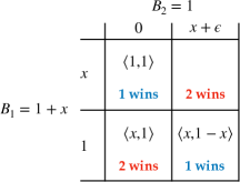
Consider the qualitative reachability game that is depicted in Fig. 1, which we call win twice in a row or , for short. For convenience, fix Player ’s initial budget to be . The solution to the game using a first-price auction is trivial: for example, with poorman bidding (in which the winner pays the bank), Player wins iff his budget exceeds . Indeed, if his budget is , he bids in the first bidding, moves the token to , and, since in first-price auctions, the loser does not pay his bid, the budgets in the next round are and , respectively. Player again bids , wins the bidding, moves the token to , and wins the game. On the other hand, if Player ’s budget is , Player can guarantee that the token reaches by bidding in both rounds.
The solution to this game with all-pay bidding is much more complicated and was posed as an open question in (?), which we completely solve. Assuming Player ’s budget is , it is easy to show that when Player ’s initial budget is either greater than or smaller than , there exist a deterministic winning strategy for one of the players. Also, for budgets in between, i.e, in , it is not hard to see that optimal strategies require probabilistic choices, which is the source of the difficulty and an immediate difference from first-price bidding rules. We characterize the value of the game, which is the optimal probability that Player can guarantee winning, as a function of Player ’s initial budget. In Theorem 5.1, we show that for and , the value is when Player ’s initial budget is and Player ’s initial budget is . Fig. 1 gives a flavor of the the solution in the simplest interesting case of , where a Player strategy that bids and each with probability guarantees winning with probability . ∎
Apart from the theoretical interest in all-pay bidding games, we argue that they are useful in practice, and that they address limitations of previously studied models. All-pay auctions are one of the most well-studied auction mechanisms (?). Even though they are described in economic terms, they are often used to model settings in which the agents’ bids represent the amount of effort they invest in a task such as in rent seeking (?), patent races, e.g., (?), or biological auctions (?). As argued in (?), however, many decision-making settings, including the examples above, are not one-shot in nature, rather they develop dynamically. Dynamic all-pay auctions have been used to analyze, for example, political campaigning in the USA (?), patent races (?), and (?) argue that they appropriately model sport competitions between two teams such as “best of ” in the NBA playoffs. An inherent difference between all-pay repeated auctions and all-pay bidding games is that our model assumes that the players’ effort has no or negligible inherent value and that it is bounded. The payoff is obtained only from the reward in the leaves. For example, a “best of ” sport competition between two sport teams can be modelled as an all-pay bidding game as follows. A team’s budget models the sum of players’ strengths. A larger budget represents a fresher team with a deeper bench. Each bidding represents a match between the teams, and the team that bids higher wins the match. The teams only care about winning the tournament and the players’ strengths have no value after the tournament is over.
The closest model in spirit is called Colonel Blotto games, which dates back to (?), and has been extensively studied since. In these games, two colonels own armies and compete in battlefields. Colonel Blotto is a one-shot game: on the day of the battle, the two colonels need to decide how to distribute their armies between the battlefields, where each battlefield entails a reward to its winner, and in each battlefield, the outnumbering army wins. To the best of our knowledge, all-pay bidding games are the first to incorporate a modelling of bounded resource with no value for the players, as in Colonel Blotto games, with a dynamic behavior, as in ongoing auctions.
Graph games have been extensively used to model and reason about systems (?) and multi-agent systems (?). Bidding games naturally model systems in which the scheduler accepts payment in exchange for priority. Blockchain technology is one such system, where the miners accept payment and have freedom to decide the order of blocks they process based on the proposed transaction fees. Transaction fees are not refundable, thus all-pay bidding is the most appropriate modelling. Manipulating transaction fees is possible and can have dramatic consequences: such a manipulation was used to win a popular game on Ethereum called FOMO3d111https://bit.ly/2wizwjj. There is thus ample motivation for reasoning and verifying blockchain technology (?).
We show that all-pay bidding games exhibit an involved and interesting mathematical structure. As discussed in Example 1.1, while we show a complete characterization of the value function for the game , it is significantly harder than the characterization with first-price bidding. The situation becomes worse when we slightly complicate the game and require that Player wins three times in a row, called , for short. We show that there are initial budgets for which an optimal strategy in requires infinite support.
We turn to describe our positive results on general games. First, we study surely-winning in all-pay bidding games, i.e., winning with probability . We show a threshold behavior that is similar to first-price bidding games: each vertex in a qualitative all-pay bidding game has a surely-winning threshold ratio, denoted , such that if Player ’s ratio exceeds , he can guarantee winning the game with probability , and if Player ’s ratio is less than , Player can guarantee winning with positive probability. Moreover, we show that surely-winning threshold ratios have the following structure: for every vertex , we have , where and are the neighbors of that, respectively, minimize and maximize SThr. This result has computation-complexity implications; namely, we show that in general, the decision-problem counterpart of finding surely-winning threshold ratios is in PSPACE using the existential theory of the reals (ETR, for short) (?), and it is in linear time for DAGs. We show that surely-winning threshold ratios can be irrational, thus we conjecture that the decision problem is sum-of-squareroot-hard.
Example 1.2.
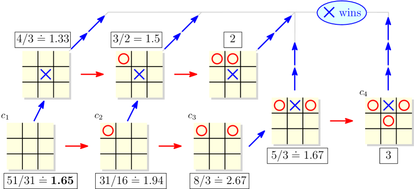
Tic-tac-toe is a canonical graph game that is played on a DAG. First-price bidding Tic-tac-toe was discussed in a blog post222https://bit.ly/2KUong4, where threshold budgets are shown to be surprisingly low: with Richman bidding, Player can guarantee winning when his ratio exceeds (?) and with poorman-bidding, when it exceeds roughly .
We implement our algorithm and find surely-winning threshold ratios in all-pay bidding tic-tac-toe: Player surely wins when his initial ratio is greater than (see Fig. 2). We point to several interesting phenomena. One explanation for the significant gap between the thresholds in all-pay and first-price bidding is that, unlike Richman and poorman bidding, in the range neither player surely wins. Second, the threshold ratio for the relaxed Player goal of surely not-losing equals the surely-winning threshold ratio. This is not always the case; e.g., from the configuration with a single in the middle left position, Player requires a budget of for surely winning and for surely not-losing. Third, we find it surprising that when Player wins the first bidding, it is preferable to set an in one of the corners (as in configuration ) rather than in the center. ∎
Finally, we devise an FPTAS for the problem of finding values in DAGs; namely, given a bidding game that is played on a DAG, an initial vertex, and an , we find, in time polynomial in the size of and , an upper- and lower-bound on the expected payoff that Player can guarantee with every initial ratio of the form . The idea is to discretize the budgets and bids and, using a bottom-up approach, repeatedly solve finite-action zero-sum games. The algorithm gives theoretical bounds on the approximation. It is a simple algorithm that we have implemented and experimented with. Our experiments show that the difference between upper- and lower-bounds is small, thus we conclude that the algorithm supplies a good approximation to the value function. The experiments verify our theoretical findings. In addition, they hint at interesting behavior of all-pay bidding games, which we do not yet understand and believe encourages a further study of this model.
Related work
Colonel Blotto games (?) have been extensively studied; a handful of papers include (?; ?; ?; ?). They have mostly been studied in the discrete case, i.e., the armies are given as individual soldiers, but, closer to our model, also in the continuous case (see (?) and references therein). The most well-studied objective is maximizing the expected payoff, though recently (?) study the objective of maximizing the probability of winning at least battlefields, which is closer to our model.
All-pay bidding games were mentioned briefly in (?), where it was observed that optimal strategies require probabilistic choices. To the best of our knowledge, all-pay bidding games (?) were studied only with discrete-bidding, which significantly simplifies the model, and in the Richman setting; namely, both players pay their bids to the other player.
First-price bidding games have been well-studied and exhibit interesting mathematical properties. Threshold ratios in reachability Richman-bidding games, and only with these bidding rules, equal values in random-turn based games (?), which are stochastic games in which in each round, the player who moves is chosen according to a coin toss. This probabilistic connection was extended and generalized to infinite-duration bidding games with Richman- (?), poorman- (?), and even taxman-bidding (?), which generalizes both bidding rules. Other orthogonal extensions of the basic model include non-zero-sum bidding games (?) and discrete-bidding games that restrict the granularity of the bids (?; ?).
There are a number of shallow similarities between all-pay games and concurrent stochastic games (?). A key difference between the models is that in all-pay bidding games, the (upper and lower) value depends on the initial ratio, whereas a stochastic game has one value. We list examples of similarities. In both models players pick actions simultaneously in each turn, and strategies require randomness and infinite memory though in Everett recursive games (?), which are closest to our model, only finite memory is required and in more general stochastic games, the infinite memory requirement comes from remembering the history e.g. (?) whereas in all-pay bidding games infinite support is already required in the game “win 3 times in a row” (which has histories of length at most ). Also, computing the value in stochastic games is in PSPACE using ETR (?), it is in P for DAGs, and there are better results for solving the guaranteed-winning case (?).
2 Preliminaries
A reachability all-pay bidding game is , where is a finite set of vertices, is a set of directed edges, is a set of leaves with no outgoing edges, and assigns unique weights to leaves, i.e., for , we have . We require that every vertex in has a path to at least two different leaves. A special case is qualitative games, where there are exactly two leaves with weights in . We say that a game is played on a DAG when there are no cycles in the graph. For , we denote the neighbors of as .
A strategy is a recipe for how to play a game. It is a function that, given a finite history of the game, prescribes to a player which action to take, where we define these two notions below. A history in a bidding game is , where for , the token is placed on vertex at round and Player ’s bid is , for . Let be the initial budget of Player . Player ’s budget following is . A play that ends in a leaf is associated with the payoff .
Consider a history that ends in . The set of legal actions following , denoted , consists of pairs , where is a bid that does not exceed the available budget and is a vertex to move to upon winning. A mixed strategy is a function that takes and assigns a probability distribution over . The support of a strategy is . We assume WLog. that each bid is associated with one vertex to proceed to upon winning, thus if , then . We say that is pure if, intuitively, it does not make probabilistic choices, thus for every history , we have .
Definition 2.1 (Budget Ratio).
Let be initial budgets for the two players. Player ’s ratio is .333We find this definition more convenient than which is used in previous papers on bidding games.
Let be an all-pay bidding game. An initial vertex , an initial ratio , and two strategies and for the two players give rise to a probability over plays, which is defined inductively as follows. The probability of the play of length is . Let , where ends in a vertex . Then, we define . Moreover, for , assuming Player chooses the successor vertex , i.e., , then when and otherwise . That is, we resolve ties by giving Player the advantage. This choice is arbitrary and does not affect most of our results, and the only affect is discussed in Remark 5.1.
Definition 2.2 (Game Values).
The lower value in an all-pay game w.r.t. an initial vertex , and an initial ratio is . The upper value, denoted is defined dually. It is always the case that , and when , we say that the value exists and we denote it by .
3 Surely-Winning Thresholds
In this section we study the existence and computation of a necessary and sufficient initial budget for Player that guarantees surely winning, namely winning with probability . We focus on qualitative games in which each player has a target leaf. Note that the corresponding question in quantitative games is the existence of a budget that suffices to surely guarantee a payoff of some , which reduces to the the surely-winning question on qualitative games by setting Player ’s target to be the leaves with weight at least . We define surely-winning threshold budgets formally as follows.
Definition 3.1 (Surely-Winning Thresholds).
Consider a qualitative game and a vertex in . The surely-winning threshold at , denoted , is a budget ratio such that:
-
•
If Player ’s ratio exceeds , he has a strategy that guarantees winning with probability .
-
•
If Player ’s ratio is less than , Player has a strategy that guarantees winning with positive probability.
To show existence of surely-winning threshold ratios, we define threshold functions, show their existence, and show that they coincide with surely-winning threshold ratios.
Definition 3.2 (Threshold functions).
Consider a qualitative game . Let be a function. For , let be such that , for every . We call a threshold function if
We start by making observations on surely-winning threshold ratios and threshold functions.
Lemma 3.1.
Consider a qualitative game , and let be a threshold function.
-
•
For , if Player ’s initial ratio exceeds , then he has a pure strategy that guarantees winning.
-
•
For , we have .
-
•
We have and the inequalities are strict when .
Proof.
For the first claim, suppose Player has a strategy that guarantees winning against any Player strategy. Suppose is mixed. Then, we construct a pure strategy by arbitrarily choosing, in each round, a bid . If Player has a strategy that guarantees winning with positive probability against , then by playing against , he wins with positive probability, contradicting the assumption that guarantees surely winning. For the second claim, suppose towards contradiction that , for . We think of Player as revealing his pure winning strategy before Player . Assuming Player bids in a round, Player reacts by bidding . Thus, Player wins biddings in a row and draws the game to . A simple calculation verifies the last claim. ∎
We first show that threshold functions coincide with surely-winning threshold ratios, and then show their existence.
Lemma 3.2.
Consider a qualitative game and let be a threshold function for . Then, for every vertex , we have ; namely, Player surely wins from when his budget exceeds .
Proof.
We claim that if Player ’s ratio is , for , he can surely-win the game. For and , the claim is trivial and vacuous, respectively. We provide a strategy for Player that guarantees that in at most steps, either Player has won or he is at some node with relative budget , where is a small fixed positive number. By repeatedly applying this strategy, either Player at some point wins directly, or he accumulates relative budget and then he can force a win in steps by simply bidding in each round.
Suppose the token is placed on vertex following biddings, let be neighbors of that achieve the minimal and maximal value of , respectively. For convenience, set , , and . Player bids . We first disregard the supplementary . When Player wins, we consider the worst case of Player bidding , thus Player ’s normalized budget is greater than . On the other hand, when Player loses, Player bids at least as much as Player , and Player ’s normalized budget is greater than .
Upon winning a bidding, Player moves to a neighbor with , and when losing, the worst case is when Player moves to a vertex with . The claim above shows that in both cases Player ’s budget exceeds . Since , we have established that the strategy guarantees not losing.
We define Player ’s moves precisely, and show how Player uses the surplus to guarantee winning. We define Player moves upon winning a bidding at . He moves to such that , where if there are several vertices that achieve the minimal value, he chooses a vertex that is closest to . By Lemma 3.1, for every vertex , we have and equality occurs only when . Thus, Player ’s move guarantees that and if is farther from than , then the inequality is strict. The sum of decreases in and in distance is at most , thus is reached after winning biddings.
We show how to use the surplus to guarantee winning. First note that and the extra terms add up to at most so the bids are legal (we assume, WLog., that ). Finally, if Player wins the -th bidding, Player ’s ratio is at least whereas Player ’s ratio is at most . Player ’s new ratio is then at least , and it is straightforward to check that this is at least as much as the desired , where . ∎
To obtain the converse, we show a strategy for Player that wins with positive probability. We identify an upper bound in each vertex such that a Player bid that exceeds exhausts too much of his budget. Then, Player bids with probability and the rest of the probability mass is distributed uniformly in . This definition intuitively allows us to reverse the quantification and assume Player reveals his strategy before Player ; that is, when Player bids at least , we consider the case that Player bids , and when Player bids less than , we consider the case where Player slightly overbids Player . Both occur with positive probability.
Lemma 3.3.
Consider a qualitative game and let be a threshold function for . Then, for every vertex , we have ; namely, Player wins with positive probability from when Player ’s budget is less than .
Proof.
We distinguish between two types of vertices in . The first type is and the second type is . Assume Player ’s budget is at least and Player ’s budget is at most . We use to denote an upper bound on Player ’s bids. For , we set , and for , we set , where is a small constant, , and is the length of the shortest path from to a vertex in the first type of vertices. Player bids with probability and the rest of the probability mass is distributed uniformly in . Upon winning, in the first case, Player moves to a vertex that is closest to , and in the second case, to a vertex that is closest to a vertex in .
Intuitively, a bid above is too high for Player since it exhausts too much of his budget. Thus, when Player bids at least , we consider the case where Player bids , and when Player bids below , we consider the case where Player bids slightly above him, both occur with positive probability. Note that in both cases, we maintain the invariant that Player ’s budget is at least and Player ’s budget is at most , thus Player does not win the game. We show that Player wins with positive probability. Consider a finite play that is obtained from some choice of strategy of Player . Note that a cycle in necessarily results from a Player win (against a Player bid of ), and such a win occurs when he bids at least . In both cases, Player ’s budget decreases by a constant. The tricky case is when the cycle is contained in . Then, the sum of Player ’s bids is at most whereas Player bids at least . Thus, Player ’s decrease in budget is larger by a factor of of Player . Thus, Player ’s budget will eventually be larger than Player ’s, at which point Player wins in at most steps since he always bids above Player ’s budget with positive probability. ∎
Finally, we show existence of threshold functions. We first show existence in DAGs, which is a simple backwards-induction argument that we have implemented (see Example 1.2). To obtain existence in a general game , we find threshold functions in games on DAGs of the form , for , in which Player is restricted to win in at most steps. We tend to infinity and show that the limit of the threshold functions in the games is a threshold function in .
Lemma 3.4.
Every qualitative reachability bidding game has a threshold function.
Proof.
Note that in a game that is played on a DAG, the existence of a threshold function is shown easily in a backwards-induction manner from the leaves. Consider a game . For let be the reachability game in which Player wins iff the game reaches in at most rounds. Since is a DAG, by the above, a threshold function exists in . By Lemma 3.2, we have , and by Lemma 3.1, we have , thus the sequence converges. We define and claim that is a threshold function.
We show that converges to . Note that since is a DAG, we have . Moreover, for , note that , since a budget of allows Player to win times in a row and draw the game to . Since is a monotonically decreasing sequence, for every , there is such that for every , we have . Given , we choose such that
∎
We use the characterization of surely-winning threshold ratios by means of threshold functions (Lemmas 3.2 and 3.3) to find the threshold ratios in the game that is depicted in Fig. 3, and show that they can be irrational. In addition the characterization has computation-complexity consequences on the problem of finding surely-winning threshold ratios. In DAGs, finding threshold functions is done in linear time. In general graphs, the characterization implies a reduction to the existential theory of the reals (ETR, for short) by phrasing the constraints in Definition 3.2 as an input to ETR. It is known that ETR is in PSPACE (?). Combining the lemmas above, we have the following.
Theorem 3.5.
Surely-winning threshold ratios exist in every qualitative reachability game and coincide with threshold functions. Surely-winning threshold ratios can be irrational. Given a vertex and a value , deciding whether is in PSPACE for general graphs and can be solved in linear time for games on DAGs.

4 Finding Approximated Values
In this section, we focus on games on DAGs. The algorithm that we construct is based on a discretization of the budgets; namely, we restrict the granularity of the bids and require Player to bid multiples of some , similar in spirit to discrete-bidding games (?). We first relate the approximated value with the value in with no restriction on the bids. Then, in Section 6, we experiment with an implementation of the algorithm and show interesting behavior of all-pay bidding games. We define the approximate value as follows.
Definition 4.1 (Approximate Value Function).
Let be a game on a DAG and . Let be the approximate-value function in when Player is restricted to choose bids in and Player wins ties.
Our algorithm is based on the following theorem.
Theorem 4.1.
Consider a game on a DAG where each leaf is labeled with a reward. Let be a vertex in , be an initial budget for Player , be the longest path from a vertex to a leaf in , and . Then, we have .
Theorem 4.1 gives rise to Algorithm 4 that finds , for every that is a multiple of . Note that assuming Player bids only multiples of , we can assume that Player also bids multiples of . The algorithm constructs a two-player zero-sum matrix game, which is , where, for , is a finite set of actions for Player , and, given , the function is the payoff of the game. A solution to the game is the optimal payoff that Player can guarantee with a mixed strategy, and it is found using linear programming. Let denote the threshold budget with which Player can guarantee the highest reward, then equals the highest reward, for . To compute , we use the linear-time algorithm in the previous section.
5 “Win in a Row” Games
In this section we study a simple fragment of qualitative games.
Definition 5.1 (Win in a Row Games).
For , let denote the qualitative game in which Player needs to win biddings in a row and otherwise Player wins. For example, see a depiction of in Fig. 1.
We start with a positive results and completely solve . Then, we show that optimal strategies require infinite support already in .
A solution to “win twice in a row”
We start by solving an open question that was posed in (?) and characterize the value as a function the budget ratio in the win twice in a row game (see a depiction of the game in Fig. 1).
Theorem 5.1.
Consider the all-pay bidding game in which Player needs to win twice and Player needs to win twice. The value exists for every pair of initial budgets. Moreover, suppose the initial budgets are for Player and for Player . Then, if , the value is , if , the value is , and if , for , then the value is .
Proof.
The cases when and are easy. Let such that , where is such that . We claim that the value of with initial budgets and is . Consider the Player strategy that choses a bid in uniformly at random. We claim that no matter how Player bids, one of the choices wins, thus the strategy guarantees winning with probability at least . Let be a Player bid and let be such that . Consider the case where Player bids and wins the first bidding. Player ’s normalized budget in the second bidding is , thus Player wins the second bidding as well. Next, we show that Player ’s strategy is optimal by showing a Player strategy that guarantees winning with probability at least . Let such that , which exists since . Player chooses a bid uniformly at random in . Suppose Player bids , and we claim that the bid wins against at most one choice of Player . Let be a Player bid. When , Player wins immediately. A simple calculation reveals that when , then Player ’s normalized budget in the second bidding is less than , thus he loses. It is not hard to see that there are choices for Player that guarantee winning. ∎
Remark 5.1.
Note that the tie-breaking mechanism affects the winner at the end-points of the intervals. For example, if we would have let Player win ties, then the intervals would have changed to .
Infinite support is required in
We continue to show a negative result already in : there is an initial Player budget for which his optimal strategy requires infinite support, which comes as a contrast to the optimal strategies we develop for , which all have finite support.
A sweeping algorithm.
In order to develop intuition for the proof, we present a sketch of an algorithm that decides, given and , whether Player can guarantee winning with probability in when his initial budget is and Player ’s budget is . We assume access to a function that, given a budget for Player , returns in . For example, Theorem 5.1 shows that , for . The algorithm constructs a sequence of strategies for Player for the first bidding, each with finite support. We define and . That is, according to , in the first bidding, Player bids with probability and with probability . Note that . For , suppose is defined, that its support is , and that , for any Player bid . Intuitively, as Player lowers his bid, his remaining budget for the subsequent biddings increases and the winning probability for Player decreases. We “sweep down” from and find the maximal bid of Player such that . We define by, intuitively, shifting some of the probability mass that assigns to to , thus and , for . We terminate in two cases. If there is no positive such that , then guarantees a value of , and we return it. On the other hand, if there is no that guarantees , then there . For example, in the game with and , we define . We find by solving to obtain , and define . Similarly, we find by solving , and terminate.
Infinite support is required.
The following lemma, shows a condition for the in-optimality of a strategy. Intuitively, consider a Player strategy that is obtained as in the sweeping algorithm only that in the -th iteration, instead of adding to the support, it adds . The value that guarantees needs to be at least for any Player bid, and specifically for and . Note that it is clearly beneficial for Player to bid rather than against the bid of Player . Since is not in the support of , the probability is un-necessarily high to “compensate”. We construct by shifting some of this probability to , we are left with a “surplus” which we re-distribute to the rest of the support of , thus guarantees a better value than . Formally, we have the following.
Lemma 5.2.
Consider a Player strategy in , for some , that has finite support in the first bidding. If there is , , and with and , then is not optimal.
Proof.
Suppose that the strategy guarantees a value of and let be as in the statement. The value is at least against any Player strategy, and in particular against the bids and , thus . We claim that , thus . Recall that the definition of the outcome is and similarly for . Fixing a Player bid, the function is monotonically decreasing with Player ’s bids since the lower Player bids, the more budget he has left for subsequent biddings. Thus, for , we have , and the assumptions of the lemma imply that at least one of the inequalities is strict. Thus, the claim follows and we have .
Next, we construct a “partial-strategy” by adding to the support. Formally, we define , for , and let be such that . Let , and let be such that . We claim that, intuitively, we are left with a “surplus”, and formally, we have . As in the above, we have . Suppose we chose the maximal for which the statement holds, thus for every , we have , and , for some . We subtract the equality from and plug in the equalities to obtain . Since we assume , the claim follows.
Let denote our “surplus”, which, by the above, is positive. We define a new Player strategy with support . The probability of , for is . The probability of is and the probability of is . It is not hard to show that guarantees a value that is greater than , thus is not optimal. ∎
Next, we use Lemma 5.2 to show that any strategy with finite support is not optimal.
Theorem 5.3.
Consider the game in which Player needs to win three biddings and Player needs to win once. Suppose the initial budgets are for Player and for Player . Then, an optimal strategy for Player requires infinite support in the first bidding.
Proof.
Suppose towards contradiction that is an optimal strategy with finite support in the first bidding. Consider the infinite sequence , for . It is not hard to verify that , for every . That is, when Player bids and Player bids , by Theorem 5.1, the value is .
Let be the support of in the first bidding, where . Since the support is finite, there is an and such that . We claim that satisfies the assumptions of Lemma 5.2, thus is not optimal. First, it is not hard to verify that for , we have . Since the sequence tends to , we have . Second, when Player ’s bid is fixed, then is monotonically decreasing with Player ’s bid, thus . Thus, , and we are done. ∎
6 Experiments
We have implemented Algorithm 4 and experiment by running it on qualitative games that are called a race in (?).
Definition 6.1 (Race Games).
For , let be the qualitative game that consists of at most biddings in which Player wins if he wins biddings and Player wins if he wins biddings. Specifically, we have .
The algorithm is implemented in Python and it is run on a personal computer. In our experiments, we choose . In terms of scalability, the running time for for solving the game is at most minutes. Solutions to smaller games are in the order of seconds to several minutes.
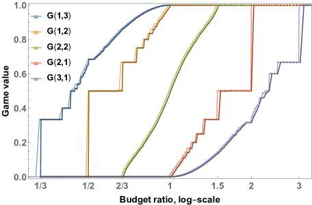
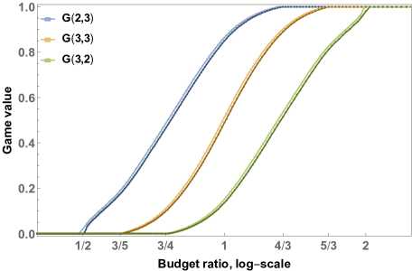
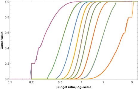
Figure 5 depicts some values for five games as output by the implementation. We make several observations. First, close plots represent the upper- and lower-bounds of a game. We find it surprising that the difference between the two approximations is very small, and conclude that the output of the algorithm is a good approximation of the real values of the games. Second, the plot of (depicted in red), is an experimental affirmation of Theorem 5.1; namely, the step-wise behavior and the values that are observed in theory are clearly visible in the plot. Third, while a step-wise behavior can be seen for high initial budgets in (depicted in purple), for lower initial budgets, the behavior seems more involved and possibly continuous. In Theorem 5.3, we show that optimal strategies for initial budgets in this region require infinite support, and the plot affirms the more involved behavior of the value function that is predicted by the theorem. Continuity is more evident in more elaborate games whose values are depicted in Figure 6. Both plots give rise to several interesting open questions, which we elaborate on in the next section.
7 Discussion
We study, for the first time, all-pay bidding games on graphs. Unlike bidding games that use variants of first-price auctions, all-pay bidding games appropriately model decision-making settings in which bounded effort with no inherent value needs to be invested dynamically. While our negative results show that all-pay bidding games are significantly harder than first-price bidding games, our results are mostly positive. We are able to regain the threshold-ratio phenomena from first-price bidding games by considering surely-winning threshold ratios, and our implementation for games on DAGs solves non-trivial games such as tic-tac-toe. We show a simple FPTAS that finds upper- and lower-bounds on the values for every initial budget ratio, which we have implemented and show that it performs very well.
We leave several open questions. The basic question on games, which we leave open, is showing the existence of a value with respect to every initial ratio in every game. We were able to show existence in , and Fig. 6 hints the value exists in more complicated games. Also, while we identify the value function in , we leave open the problem of a better understanding of this function in general. For example, while for we show that it is a step-wise function, observing Fig. 6 it seems safe to guess that the function can be continuous. Finally, characterizing the function completely, similar to our solution of , in more involved games, is an interesting and challenging open problem.
8 Acknowledments
This research was supported by the Austrian Science Fund (FWF) under grants S11402-N23 (RiSE/SHiNE), Z211-N23 (Wittgenstein Award), and M 2369-N33 (Meitner fellowship).
References
- [Aghajohari, Avni, and Henzinger 2019] Aghajohari, M.; Avni, G.; and Henzinger, T. A. 2019. Determinacy in discrete-bidding infinite-duration games. In Proc. 30th CONCUR, volume 140 of LIPIcs, 20:1–20:17.
- [Avni, Henzinger, and Chonev 2019] Avni, G.; Henzinger, T. A.; and Chonev, V. 2019. Infinite-duration bidding games. J. ACM 66(4):31:1–31:29.
- [Avni, Henzinger, and Ibsen-Jensen 2018] Avni, G.; Henzinger, T. A.; and Ibsen-Jensen, R. 2018. Infinite-duration poorman-bidding games. In Proc. 14th WINE, volume 11316 of LNCS, 21–36. Springer.
- [Avni, Henzinger, and Žikelić 2019] Avni, G.; Henzinger, T. A.; and Žikelić, Đ. 2019. Bidding mechanisms in graph games. In In Proc. 44th MFCS, volume 138 of LIPIcs, 11:1–11:13.
- [Baye and Hoppe 2003] Baye, M. R., and Hoppe, H. C. 2003. The strategic equivalence of rent-seeking, innovation, and patent-race games. Games and Economic Behavior 44(2):217–226.
- [Behnezhad et al. 2019] Behnezhad, S.; Blum, A.; Derakhshan, M.; Hajiaghayi, M. T.; Papadimitriou, C. H.; and Seddighin, S. 2019. Optimal strategies of blotto games: Beyond convexity. In Proc. the 20th EC, 597–616.
- [Bellman 1969] Bellman, R. 1969. On “colonel blotto” and analogous games. SIAM Rev. 11(1):66–68.
- [Blackett 1954] Blackett, D. W. 1954. Some blotto games. NRL 1(1):55–60.
- [Borel 1921] Borel, E. 1921. La théorie du jeu les équations intégrales á noyau symétrique. Comptes Rendus de l’Académie 173(1304–1308):58.
- [Canny 1988] Canny, J. F. 1988. Some algebraic and geometric computations in PSPACE. In Proc. 20th STOC, 460–467.
- [Chatterjee and Ibsen-Jensen 2015] Chatterjee, K., and Ibsen-Jensen, R. 2015. The value 1 problem under finite-memory strategies for concurrent mean-payoff games. In Proc. 26th SODA, 1018–1029.
- [Chatterjee, Goharshady, and Velner 2018] Chatterjee, K.; Goharshady, A. K.; and Velner, Y. 2018. Quantitative analysis of smart contracts. In Proc. 27th ESOP, 739–767.
- [Chatterjee, Reiter, and Nowak 2012] Chatterjee, K.; Reiter, J. G.; and Nowak, M. A. 2012. Evolutionary dynamics of biological auctions. Theoretical Population Biology 81(1):69 – 80.
- [Clarke et al. 2018] Clarke, E. M.; Henzinger, T. A.; Veith, H.; and Bloem, R., eds. 2018. Handbook of Model Checking. Springer.
- [Develin and Payne 2010] Develin, M., and Payne, S. 2010. Discrete bidding games. The Electronic Journal of Combinatorics 17(1):R85.
- [Etessami et al. 2008] Etessami, K.; Kwiatkowska, M. Z.; Vardi, M. Y.; and Yannakakis, M. 2008. Multi-objective model checking of markov decision processes. LMCS 4(4).
- [Everett 1955] Everett, H. 1955. Recursive games. Annals of Mathematics Studies 3(39):47–78.
- [Harris and Vickers 1985] Harris, C., and Vickers, J. 1985. Perfect equilibrium in a model of a race. The Review of Economic Studies 52(2):193 – 209.
- [Hart 2008] Hart, S. 2008. Discrete colonel blotto and general lotto games. International Journal of Game Theory 36(3):441–460.
- [Klumppa and K.Polborn 2006] Klumppa, T., and K.Polborn, M. 2006. Primaries and the new hampshire effect. Journal of Public Economics 90(6–7):1073–1114.
- [Konrad and Kovenock 2009] Konrad, K. A., and Kovenock, D. 2009. Multi-battle contests. Games and Economic Behavior 66(1):256–274.
- [Lazarus et al. 1996] Lazarus, A. J.; Loeb, D. E.; Propp, J. G.; and Ullman, D. 1996. Richman games. Games of No Chance 29:439–449.
- [Lazarus et al. 1999] Lazarus, A. J.; Loeb, D. E.; Propp, J. G.; Stromquist, W. R.; and Ullman, D. H. 1999. Combinatorial games under auction play. Games and Economic Behavior 27(2):229–264.
- [Meir, Kalai, and Tennenholtz 2018] Meir, R.; Kalai, G.; and Tennenholtz, M. 2018. Bidding games and efficient allocations. Games and Economic Behavior.
- [Menz, Wang, and Xie 2015] Menz, M.; Wang, J.; and Xie, J. 2015. Discrete all-pay bidding games. CoRR abs/1504.02799.
- [Mertens and Neyman 1981] Mertens, J., and Neyman, A. 1981. Stochastic games. International Journal of Game Theory 10(2):53–66.
- [Michael R. Baye and de Vries 1996] Michael R. Baye, D. K., and de Vries, C. G. 1996. The all-pay auction with complete information. Economic Theory 8(2):291–305.
- [Peres et al. 2009] Peres, Y.; Schramm, O.; Sheffield, S.; and Wilson, D. B. 2009. Tug-of-war and the infinity laplacian. J. Amer. Math. Soc. 22:167–210.
- [Roberson 2006] Roberson, B. 2006. The colonel blotto game. Economic Theory 29(1):1–24.
- [Shapley 1953] Shapley, L. S. 1953. Stochastic games. Proceedings of the National Academy of Sciences 39(10):1095–1100.
- [Shubik and Weber 1981] Shubik, M., and Weber, R. J. 1981. Systems defense games: Colonel blotto, command and control. NRL 28(2):281 – 287.
- [Tullock 1980] Tullock, G. 1980. Toward a Theory of the Rent Seeking Society. College Station: Texas A&M Press. chapter Efficient rent seeking, 97–112.
- [Wooldridge et al. 2016] Wooldridge, M. J.; Gutierrez, J.; Harrenstein, P.; Marchioni, E.; Perelli, G.; and Toumi, A. 2016. Rational verification: From model checking to equilibrium checking. In Proc. of the 30th AAAI, 4184–4191.