Dual affine moment invariants

Abstract

Affine transformation is one of the most common transformations in nature, which is an important issue in the field of computer vision and shape analysis. And affine transformations often occur in both shape and color space simultaneously, which can be termed as Dual-Affine Transformation (DAT). In general, we should derive invariants of different data formats separately, such as 2D color images, 3D color objects, or even higher-dimensional data. To the best of our knowledge, there is no general framework to derive invariants for all of these data formats. In this paper, we propose a general framework to derive moment invariants under DAT for objects in $M$-dimensional space with $N$ channels, which can be called dual-affine moment invariants (DAMI). Following this framework, we present the generating formula of DAMI under DAT for 3D color objects. Then, we instantiated a complete set of DAMI for 3D color objects with orders and degrees no greater than 4. Finally, we analyze the characteristic of these DAMI and conduct classification experiments to evaluate the stability and discriminability of them. The results prove that DAMI are robust for DAT. Our derivation framework can be applied to data in any dimension with any number of channels.

1 Introduction

The world we live in is so rich and varied. But there must be some invariable factors that enable people to identify the same object from the change. Among these complex transformations in nature, affine transformation is one of the most basic and common issue in computer vision, which is the largest set of linear transformations, including rotation, translation, scaling, et cetera. Geometric affine transformation in shape space can be used to approximate the projective transformations in images where the camera happened a slight change of viewing perspective, which is the most common situation in the imaging process. Photometric affine transformation in channel space is the best linear model to describe the color degradation of the outdoor scenes, which has been proved in Geusebroek et al. (2001). And affine transformations often occur in both shape and color space simultaneously, which can be termed as Dual-Affine Transformation (DAT). DAT is a useful and common transformation model to describe the degradations happened in vision information from our diverse and colorful world, which considering both shape and color degradation. Invariants under DAT is a kind of important image feature that can be used for object classification and object retrieval.

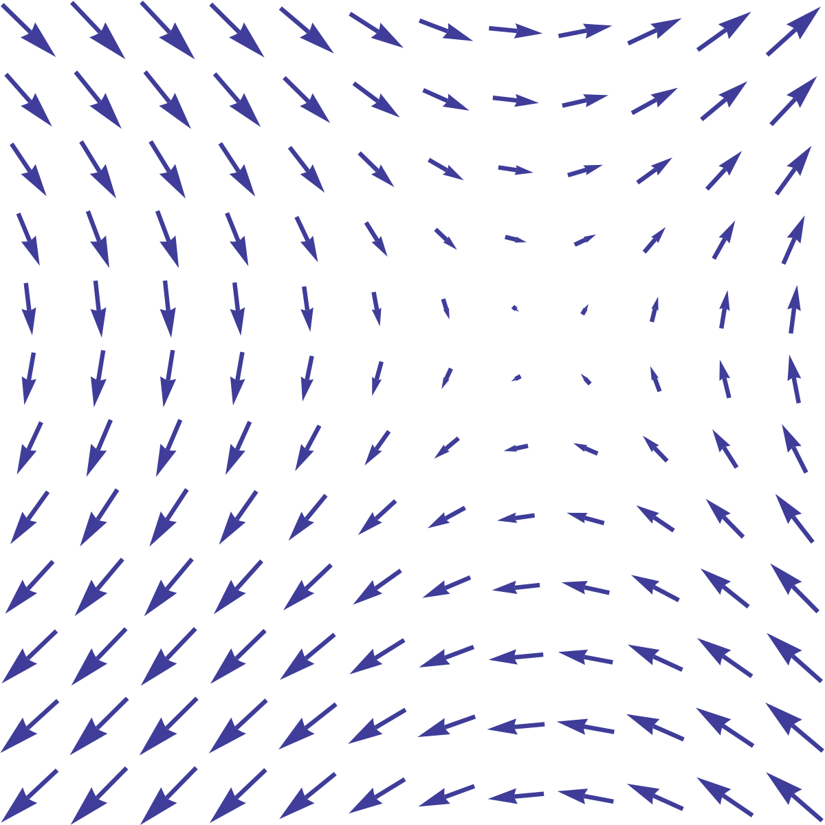
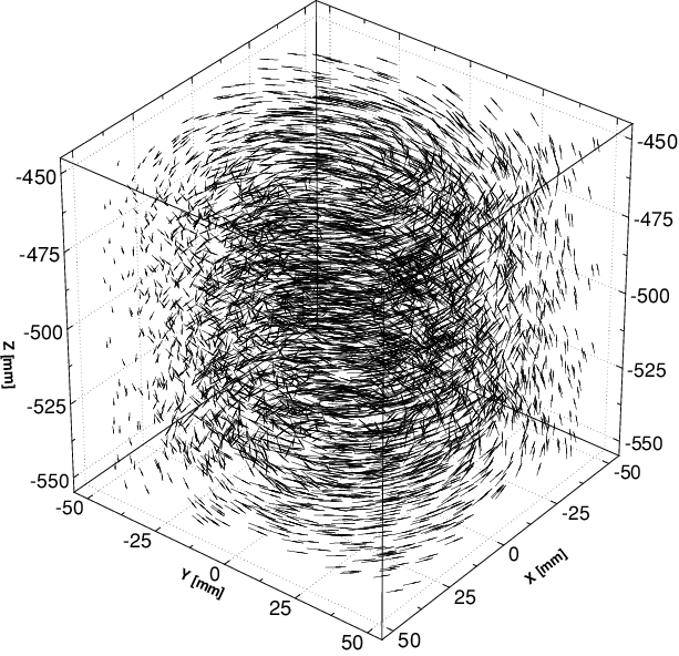
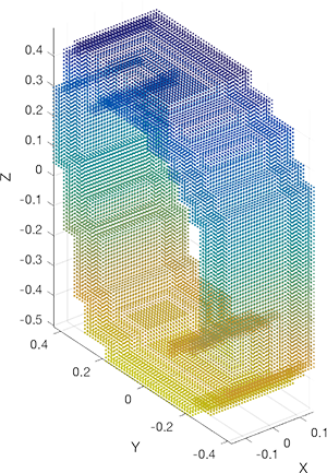
With the diversification of visual data acquisition means, the formats of visual data are also diversified, which exist in different dimension and with different number of color channels, such as 2D color images, 3D color objects, 4D movies of a 3D color object, even higher-dimensional data and multi-spectrum images with multi-channels. Other data organized in channels (such as vector fields) can also be included in this work. Some examples are shown in Figure 1.

In common, we can derive dual-affine moment invariants for objects in a particular dimension with a certain number of channels separately. To the best of our knowledge, there is no general framework to derive invariants for all of these data formats. In this paper, we systematically analyze the properties of invariants under DAT for different data dimensions and present a general framework for deriving invariants under DAT for objects in $M$-dimensional shape space with $N$ color channels.

1.1 Object definition in $M$-dimensional space with $N$ channels

An object in $M$-dimensional ($M$-D) shape space, ($X,Y,Z,S4,S5,...$), with $N$ channels, ($R,G,B,C4,C5,...$), can be described as Equation (1):

$$O_{M,N}=f_{M,N}(\vec{X})=( R(\vec{X});G(\vec{X});B(\vec{X});C4(\vec{X});C5(\vec{X});...)$$ (1)

where $\vec{X}$ represents the coordinate $(x,y,z,s4,s5,...)^{T}$ in $M$-D space. And $R(\cdot),G(\cdot),B(\cdot),C4(\cdot),C5(\cdot)$ represent the functions in different channels. Object $O$ can be defined in another form as Equation (1.1):

$$O_{M,N}(id)= [S_{M}(id),C_{N}(id)]$$

$$= [(x_{id},y_{id},z_{id},s4_{id},s5_{id},...)^{T},(r_{id},g_{id},b_{id},c4_{id},c5_{id}...)^{T}]$$ (2)

where $id$ represents the index of pixels of object $O$. $S_{M}$ represents the coordinate in shape space and $C_{N}$ represents the values in channel space.

Lots of data are organized in channel forms, which can represent different meanings in different data, such colors in color objects and vectors in vector fields. When we specify $M,N$ to different values, we can get different data formats. For examples, gray image is object in 2D space with 1 channel where $M=2,N=1$. 2D vector field can be regarded as object in 2D space with 2 channels where $M=2,N=2$. The values of 2 channels represent the vector at each point. Color image is object in 2D space with 3 channels where $M=2,N=3$. Both 3D vector field and 3D Point Cloud are objects in 3D space with 3 channels. The difference is that values of 3 channels in 3D vector field represent the vector at each point and that in 3D Point Cloud represent the color at each point. Some objects in different formats are in Figure 1.

Figure 1: Examples of different data formats: (a) Gray image in 2D space with 1 channel ($M=2,N=1$); (b) Vector field in 2D space ($M=2,N=2$); (c) Color image in 2D space with 3 channels ($M=2,N=3$); (d) Vector field in 3D space ($M=3,N=3$); (e) Color object in Point Cloud in 3D space with 3 channels ($M=3,N=3$).

1.2 Dual-Affine Transformation (DAT)

The definition of $M$-D Affine Transformation Matrix (ATM) is listed in Equation (3), which is a $M\times M$ matrix:

$$ATM_{M}=\left(\begin{array}[]{ccccc}a_{11}&a_{12}&a_{13}&...&a_{1M}\\ a_{21}&a_{22}&a_{23}&...&a_{2M}\\ a_{31}&a_{32}&a_{33}&...&a_{3M}\\ \vdots&\vdots&\vdots&\ddots&\vdots\\ a_{M1}&a_{M2}&a_{M3}&...&a_{MM}\\ \end{array}\right)_{M\times M}$$ (3)

After $M$-D affine transformation, the coordinates of object pixels in space $S_{M}=(x,y,z,s4,s5,...,sM)^{T}$ should be transformed to $S^{*}_{M}=(x^{*},y^{*},z^{*},s4^{*},s5^{*},...sM^{*})^{T}$, which can be expressed by Equation (4):

$$S^{*}_{M}=\left(\begin{array}[]{c}x^{*}\\ y^{*}\\ z^{*}\\ s4^{*}\\ s5^{*}\\ ...\\ sM^{*}\end{array}\right)=ATM_{M}\cdot\left(\begin{array}[]{c}x\\ y\\ z\\ s4\\ s5\\ ...\\ sM\end{array}\right)=ATM_{M}\cdot S_{M}$$ (4)

After $N$-D affine transformation, the pixel values at different channels $C_{N}=(r,g,b,c4,c5,...)^{T}$ will be transformed to $C^{*}_{N}=(r^{*},g^{*},b^{*},c4^{*},c5^{*},...)^{T}$ in the same way as Equation (5):

$$C^{*}_{N}=ATM_{N}\cdot C_{N}$$ (5)

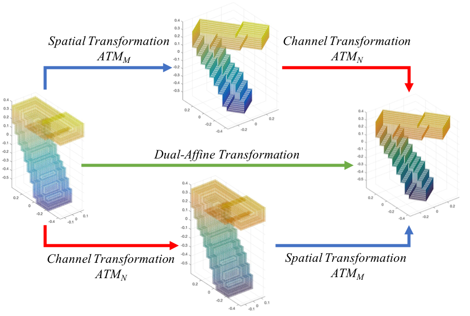
Affine transformations in shape space and channel space often occur simultaneously, which can be called Dual-Affine Transformation (DAT). DAT is the transformation we focus on in this article. The formal definition of DAT for $M$-D objects with $N$ channels can be described as Equation (6):

$$f^{*}_{M,N}(\vec{X})=ATM_{N}\cdot f_{M,N}(ATM_{M}^{-1}\cdot\vec{X})$$ (6)

where $ATM_{M}$ is the Spatial Transformation and $ATM_{N}$ is the Channel Transformation. We depict the relationship between them with DAT in Figure 2. DAT is equivalent to applying a Spatial Transformation and a Channel Transformation on the object independently.

Figure 2: The relationship between Spatial Transformation, Channel Transformation and DAT with an example of a 3D color Point Cloud ($M=3,N=3$).

One typical case of DAT is for color images, where $M=2,N=3$. The 2D geometric affine transformation in space represents the deformation of object’s shape in the images, and the 3D photometric affine transformation in channel space represents the deformation of object’s color. Moment invariants under DAT of color images has been fully discussed in Gong et al. (2017). Another case is invariants under DAT in 2D vector fields, which have been presented in Schlemmer et al. (2007); Kostková et al. (2018); Kostkova et al. (2019). There are also researches about 3D moment invariants under single affine transformation for 3D objects with one channel in Lo and Don (1989); Xu and Li (2008). However, with the continuous advancement of data acquisition methods, more and more forms of data have emerged, like 3D color objects, 4D or higher-dimensional data, multi-spectral images with more than 3 channels, etc. Invariant descriptors under dual-affine transformations in these domains are highly desirable.

The main contribution of this paper is that, we present a general framework for the derivation of moment invariants under DAT for $M$-dimensional objects with $N$ channels. And with this framework, we get a set of independent and usable DAMI for 3D color objects with 3 channels. The paper is organized as follows. First, we give a survey of relevant literature about DAMI in Section 2. In Section 3, we illuminate the DAMI’s derived framework in detail and get the DAMI generation formula for objects in any data format. In Section 4, we instantiate DAMI with data format of 3D color point cloud as an example. Through a visual approach, we generate a complete set of DAMI equations with $M=3,N=3$. We perform independent analysis on all DAMI equations and obtain a set of independent DAMI. In Section 5, we evaluate the ability of DAMI through numerical experiments on several data sets.

2 Related Works

Moment invariants were introduced into visual pattern recognition by Hu (1962) for character recognition, which are invariant under 2D similarity transformation. These seven invariants are considered as a kind of shape descriptor, which plays an important role in the field of pattern recognition. Since then, various kinds of moment invariants have been proposed for different data formats. Researchers in this field mainly focus on the following three directions: (i) The first is to extend the transform group of invariants to more complex ones. (ii) The second is to derive invariants for data of different dimensions or formats. (iii) The third is to derive invariants including both shape and color degradations into consideration.

For gray-scale images, Flusser and Suk extended Hu’s moment invariants into affine transformation in Flusser and Suk (1993), which are more common in nature than similar transformation. Relevant works are also demonstrated in Flusser and Suk (1994); Suk and Flusser (2004a, 2011). Invariants under projective transformation, which is the exact transformation model of the imaging process, has been analyzed in Weiss (1988); Suk and Flusser (2004b); Li et al. (2018). There are also some other interesting transformations that not only for image data. Invariants under these transformations are also an important direction in the field, like chiral invariants in Zhang et al. (2017), invariants under Möbius transformation in Zhang et al. (2018), and even some researches about invariants under conformal, quasi-conformal, and diffeomorphism transformations in White (1973); Willmore (2000); Zeng and Gu (2011); Rustamov et al. (2013). Invariant primitive is the most important part of the derivation process of invariants and is the essential invariant property under a certain transform group. Invariant construction frameworks are always based on primitives. Under affine transformation in 2D space, the cross-product of the coordinates of two points is the covariant primitive, which is used to derive affine invariant for gray-scale images in Suk and Flusser (2004a). In Xu and Li (2008), the distances, areas and volumes of coordinates of points are considered as the covariant primitives for different transformations. The essential primitive under affine transformation in $n$-D space is considered as the determination of the coordinates of $n$ pixels in Mamistvalov (1998). It is the same but different format with the area of triangle in 2D space and the volume of tetrahedron in 3D space. Li et al. (2017) analysis the generating formula of invariants under different transformations in detail, which can be considered as the Shape-DNA.

There are some researches extend moment invariants into different data formats. Some works analyze shape features by extracting invariants for curves in 2D space like Mundy et al. (1992); Zhao and Chen (1997). For the 3D objects with one channel, researches about 3D affine moment invariants can be found in Lo and Don (1989); Novotni and Klein (2003); Xu and Li (2008). The invariant for n-D space has been studied in Mamistvalov (1998).

Color information is important for the recognition of objects. Some color descriptors are simple and useful for applications, like color histogram in Funt and Finlayson (1995), and color moment in Stricker and Orengo (1995). But they do not consider the color degradation model in reality. Some other color descriptors consider the degradation model of illumination, like works in Gevers and Smeulders (1999); Li et al. (2009); Gong et al. (2013). To consider shape and color degradation in the same framework, there are lots of works. Mindru et al. (2004) proposed a kind of color moment invariant with Lie group method for only color diagonal transformation. Gong et al. (2017) proposed moment invariants under dual-affine transformation for 2D color images. Some other invariants for color images can be found in Alferez and Wang (1999); Mindru et al. (2004); Suk and Flusser (2009); Mo et al. (2017). Affine transformation is considered as the best model to describe the outdoor color degradation statistically in Geusebroek et al. (2001). In this paper, we will present a general framework for the derivation of moment invariants under dual-affine transformation for $M$-D objects with $N$ channels. And with 3D color point cloud as an example, we get a set of independent and usable DAMI with $M=3,N=3$.

3 Dual-Affine Moment Invariants (DAMI)

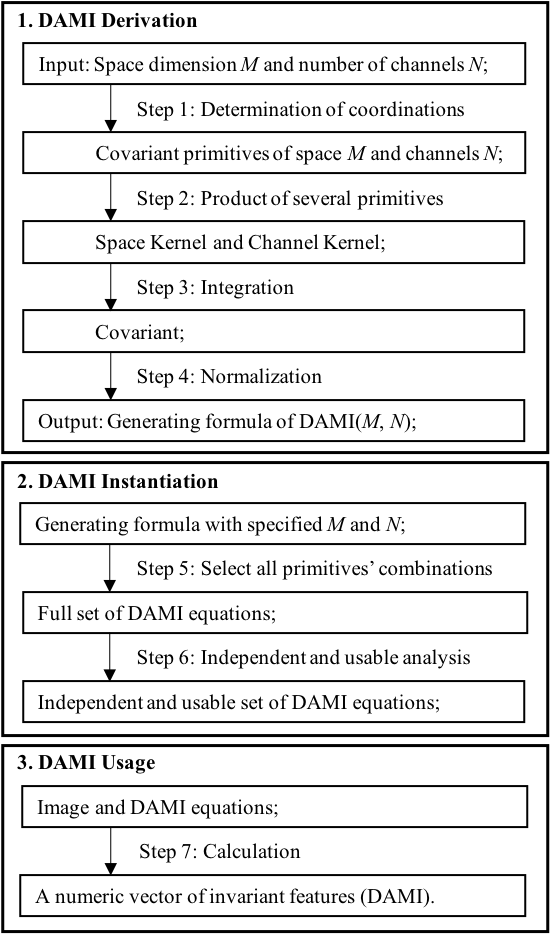
The flowchart of the derivation, instantiation, and usage of DAMI is depicted in Figure 3. We will detail the DAMI derivation framework in this section and leave the instantiation and usage part in Section 4 and 5. The general derivation framework for moment invariants is to first find the covariant primitive under a given transformation, and then derive the invariants in the global domain through the integral framework and the normalization factor. Firstly, we give the definition of covariant primitive (Step 1) in Section 3.1 and corresponding $SpaceKernel$ and $ChannelKernel$ under $M$-D affine transformation (Step 2) in Section 3.2. With the proposed $SpaceKernel$ and $ChannelKernel$, we can derive the moment covariants under DAT (Step 3) through integration in Section 3.3. In Section 3.4, we get the generating formula of DAMI after applied normalization (Step 4). Finally, we analysis the null space and a special case of DAMI In Section 3.5 and 3.6.

Figure 3: The flowchart of DAMI derivation, instantiation and usage.

3.1 Covariant primitive

Theorem 1

The matrix determinant of the coordinates of $M$ points in $M$-D space is an affine covariant primitive.

The determinant of coordinates of $M$ points in $M$-D space, $(x_{1},y_{1},z_{1},(s4)_{1},...,(sM)_{1})^{T}$, $(x_{2},y_{2},z_{2},(s4)_{2},...,(sM)_{2})^{T}$, …, $(x_{M},y_{M},z_{M},(s4)_{M},...,(sM)_{M})^{T}$, is the covariant primitive $P_{S}(M)$ in shape space as Equation (7):

$$P_{S}(M)=\det(MS(M))=\left|\begin{array}[]{cccc}x_{1}&x_{2}&\cdots&x_{M}\\ y_{1}&y_{2}&\cdots&y_{M}\\ z_{1}&z_{2}&\cdots&z_{M}\\ (s4)_{1}&(s4)_{2}&\cdots&(s4)_{M}\\ \vdots&\vdots&\ddots&\vdots\\ (sM)_{1}&(sM)_{2}&\cdots&(sM)_{M}\\ \end{array}\right|$$ (7)

After $M$-D affine transformation $ATM(M)$, the transformed $P_{S}^{*}(M)$ will be Equation (3.1):

$$P_{S}^{*}(M) =\left|MS(M)^{*}\right|=\left|ATM(M)\cdot MS(M)\right|$$

$$=\left|ATM(M)\right|\cdot\left|MS(M)\right|=\left|ATM(M)\right|\cdot P_{S}(M)$$ (8)

where $MS(M)^{*}$ is the matrix of the transformed coordinates as Equation (9):

$$MS(M)^{*}=\left(\begin{array}[]{cccc}x_{1}^{*}&x_{2}^{*}&\cdots&x_{M}^{*}\\ y_{1}^{*}&y_{2}^{*}&\cdots&y_{M}^{*}\\ z_{1}^{*}&z_{2}^{*}&\cdots&z_{M}^{*}\\ (s4)_{1}^{*}&(s4)_{2}^{*}&\cdots&(s4)_{M}^{*}\\ \vdots&\vdots&\ddots&\vdots\\ (sM)_{1}^{*}&(sM)_{2}^{*}&\cdots&(sM)_{M}^{*}\\ \end{array}\right)$$ (9)

From the result we can see that the determinant before and after the transformation only differs by one scalar coefficient, which is the determinant of the transformation matrix $ATM(M)$. $P_{S}(M)$ is a covariant primitive in $M$-D space. Theorem 1 is proved.

And similarly, in $N$-D channel space, the matrix determinant of $N$ points with $N$ channels, $(r_{1},g_{1},b_{1},(c4)_{1},...,(cN)_{1})^{T}$, $(r_{2},g_{2},b_{2},(c4)_{2},...,(cN)_{2})^{T}$, …, $(r_{N},g_{N},b_{N},(c4)_{N},...,(cN)_{N})^{T}$, is covariant primitive in channel space as Equation (10):

$$P_{C}(N)=\det(MC(N))$$ (10)

where $MC(N)$ is the matrix of the channels’ values of $N$ points. And after $N$-D affine transformation, the transformed $P^{*}_{C}(N)$ will be Equation (3.1):

$$P_{C}^{*}(N) =\left|MC(N)^{*}\right|=\left|ATM(N)\cdot MC(N)\right|$$

$$=\left|ATM(N)\right|\cdot\left|MC(N)\right|=\left|ATM(N)\right|\cdot P_{C}(N)$$ (11)

From the results, we can see that the matrix determinant $P_{C}(N)$ is covariant under affine transformation $ATM(N)$ in $N$-D channel space.

3.2 Space Kernel and Channel Kernel

Further, the continued product of several these covariant primitives is also covariant, as shown in Equation (12, 13).

$$SpaceKernel(M,P,O_{S})=\prod_{i}P_{S}(M_{i})^{t_{i}}$$ (12)

$$ChannelKernel(N,Q,O_{C})=\prod_{j}P_{C}(N_{j})^{t_{j}}$$ (13)

In which, $M_{i}$ and $N_{j}$ represent $M$ or $N$ different points and different $i$ and $j$ represent different combinations of points. All points involved in building $SpaceKernel$ constitute the Point Set $PS_{S}$. And all points involved in building $ChannelKernel$ constitute the Point Set $PS_{C}$. The number of points in the point set, $P=\left|PS_{S}\right|$ and $Q=\left|PS_{C}\right|$, are called the degree. And $t_{i}$ and $t_{j}$ are the order of corresponding primitives separately. And the $O_{S}=\sum t_{i}$ and $O_{C}=\sum t_{j}$ are called the order.

3.3 Covariant through integration

To define the $Covariant$ on object $O_{M,N}$, we make an integration of the $SpaceKernel$ and $ChannelKernel$ as Equation (3.3):

$$Covariant(M,N,P,Q,O_{S},O_{C})(O)$$

$$\quad=\iint...\iint SpaceKernel(M,P,O_{S})\cdot$$

$$\quad\quad\quad\quad\quad\quad\quad\quad ChannelKernel(N,Q,O_{C})\cdot$$

$$\quad\quad\quad\quad\quad\quad\quad\quad dx_{1}dy_{1}dz_{1}.......dx_{L}dy_{L}dz_{L}...$$ (14)

where $L=|PS_{S}\cup PS_{C}|$.

The relationship between $Covarinat$ before and after $M$-D shape affine and $N$-D channel affine transformation is in Equation (3.3):

$$Covariant^{*}(M,N,P,Q,O_{S},O_{C})(O^{*})$$

$$\quad=\iint...\iint\prod_{i}P^{*}_{S}(M_{i})^{t_{i}}\cdot\prod_{j}P^{*}_{C}(N_{j})^{t_{j}}\cdot$$

$$\quad\quad\quad\quad\quad\quad\quad\quad dx_{1}^{*}dy_{1}^{*}dz_{1}^{*}.......dx_{L}^{*}dy_{L}^{*}dz_{L}^{*}...$$

$$\quad=\left|ATM(M)\right|^{O_{S}+L}\cdot\left|ATM(N)\right|^{O_{C}}\cdot$$

$$\qquad\iint...\iint\prod_{i}P_{S}(M_{i})^{t_{i}}\cdot\prod_{j}P_{C}(N_{j})^{t_{j}}\cdot$$

$$\quad\quad\quad\quad\quad\quad\quad\quad dx_{1}dy_{1}dz_{1}.......dx_{L}dy_{L}dz_{L}...$$

$$\quad=\left|ATM(M)\right|^{O_{S}+L}\cdot\left|ATM(N)\right|^{O_{C}}\cdot$$

$$\qquad\qquad Covariant(M,N,P,Q,O_{S},O_{C})(O)$$ (15)

We can see that the difference between $Covariant$ and $Covariant^{*}$ is only one scalar coefficient, which dependents on the transformation matrix $ATM(M)$ and $ATM(N)$. The $Covariant$ is covariant under DAT.

3.4 Invariant through normalization

To achieve $Invariant$ on object $O_{M,N}$, we should eliminate the covariant scalar of the $Covariant$. We use a $NormalizationFactor$ consists of some special $Covariant$ to divide the $Covariant$ in Equation (3.3). Then we will get $Invariant$ under DAT in $M$-D space with $N$ channels as Equation (3.4):

$$Invariant(M,N,P,Q,O_{S},O_{C})(O)$$

$$\qquad=\frac{Covariant(M,N,P,Q,O_{S},O_{C})}{NormalizationFactor}$$

$$\qquad=\frac{Covariant(M,N,P,Q,O_{S},O_{C})}{\left\{\displaystyle\begin{multlined}Covariant(M,N,1,0,0,0)^{O_{S}+L-N\cdot O_{C}/2}\cdot\\ Covariant(M,N,1,N,0,2)^{O_{C}/2}\end{multlined}Covariant(M,N,1,0,0,0)^{O_{S}+L-N\cdot O_{C}/2}\cdot\\ Covariant(M,N,1,N,0,2)^{O_{C}/2}\right\}}$$ (18)

The degree is $L=|PS_{S}\cup PS_{C}|$, and the order is $K=O_{S}+O_{C}$. The $NormalizationFactor$ can be any other one that can eliminate the covariant scalar in the numerator.

This definition can be proved in Equation (3.4):

$$Invariant^{*}(M,N,P,Q,O_{S},O_{C})(O^{*})$$

$$=\frac{Covariant^{*}(M,N,P,Q,O_{S},O_{C})}{\left\{\displaystyle\begin{multlined}Covariant^{*}(M,N,1,0,0,0)^{O_{S}+L-N\cdot O_{C}/2}\cdot\\ Covariant^{*}(M,N,1,N,0,2)^{O_{C}/2}\end{multlined}Covariant^{*}(M,N,1,0,0,0)^{O_{S}+L-N\cdot O_{C}/2}\cdot\\ Covariant^{*}(M,N,1,N,0,2)^{O_{C}/2}\right\}}$$ (21)

$$=\frac{\left\{\displaystyle\begin{multlined}\left|ATM(M)\right|^{O_{S}+L}\cdot\left|ATM(N)\right|^{O_{C}}\cdot\\ Covariant(M,N,P,Q,O_{S},O_{C})\end{multlined}\left|ATM(M)\right|^{O_{S}+L}\cdot\left|ATM(N)\right|^{O_{C}}\cdot\\ Covariant(M,N,P,Q,O_{S},O_{C})\right\}}{\left\{\displaystyle\begin{multlined}(\left|ATM(M)\right|Covariant(M,N,1,0,0,0))^{O_{S}+L-N\cdot O_{C}/2}\cdot\\ (\left|ATM(M)\right|^{N}\cdot\left|ATM(N)\right|^{2}Covariant(M,N,1,N,0,2))^{O_{C}/2}\end{multlined}(\left|ATM(M)\right|Covariant(M,N,1,0,0,0))^{O_{S}+L-N\cdot O_{C}/2}\cdot\\ (\left|ATM(M)\right|^{N}\cdot\left|ATM(N)\right|^{2}Covariant(M,N,1,N,0,2))^{O_{C}/2}\right\}}$$ (26)

$$=\frac{Covariant(M,N,P,Q,O_{S},O_{C})}{\left\{\displaystyle\begin{multlined}Covariant(M,N,1,0,0,0)^{O_{S}+L-N\cdot O_{C}/2}\cdot\\ Covariant(M,N,1,N,0,2)^{O_{C}/2}\end{multlined}Covariant(M,N,1,0,0,0)^{O_{S}+L-N\cdot O_{C}/2}\cdot\\ Covariant(M,N,1,N,0,2)^{O_{C}/2}\right\}}$$ (29)

$$=Invariant(M,N,P,Q,O_{S},O_{C})(O)$$ (30)

The invariants before and after the transformation are completely equal. $Invariant(M,N,P,Q,O_{S},O_{C})$ is invariant under DAT in the $M$-D space with $N$ channels, which can be called Dual-Affine Moment Invariants ($DAMI(M,N)$).

3.5 Null space of DAMI

As we can see from the definition of covariant primitive in Equation (7) and (10), when the determinant of all primitives equal to 0, the DAMI will be no definition, which can be called the null space of DAMI.

When the null space happened in the primitives in shape space, it means matrix of the coordinations is singular. And some axis is linear combination of the other axises. The object will be part of a low-dimensional hyperplane in the original space, where the DMAI has no definition. For this kind of objects, we can find all the independent axises first, say there are $M^{\prime}$ , and then derive $DAMI(M^{\prime},N)$ on these axises. That will make the DAMI work again.

When the null space happened in the primitives in channel space, it will be the same with that in shape space. Some channels are linear dependent on others. We can find all the independent channels, say there are $N^{\prime}$, and then derive $DAMI(M,N^{\prime})$ on these independent channels. That will make the DAMI work again. The literature Kostková and Flusser (2019) has discussed some about the null space of color space. This situation is rarely seen in RGB images, but may exist in multi-spectral images.

3.6 Special case

When $M=2,N=2$, $DAMI(2,2)$ can be used on 2D vector fields with 2 channels. The $ATM(M)$ will be the coordinate transformation of the vector field and the $ATM(N)$ will be the vector transformation at each point. The DAMI will be as Equation (3.6):

$$DAMI(2,2)=Invariant(2,2,P,Q,O_{S},O_{C})(O)=$$

$$\qquad=\frac{Covariant^{*}(2,2,P,Q,O_{S},O_{C})}{\left\{\displaystyle\begin{multlined}Covariant^{*}(2,2,1,0,0,0)^{O_{S}+L-O_{C}}\cdot\\ Covariant^{*}(2,2,1,2,0,2)^{O_{C}/2}\end{multlined}Covariant^{*}(2,2,1,0,0,0)^{O_{S}+L-O_{C}}\cdot\\ Covariant^{*}(2,2,1,2,0,2)^{O_{C}/2}\right\}}$$ (33)

When select the same parameters with that in Kostková et al. (2018); Kostkova et al. (2019), we can get the same invariants as Equation (3.6).

$$DAMI(2,2)(1)=u_{0101}*u_{1010}-u_{0110}*u_{1001}$$

$$DAMI(2,2)(2)=u_{0301}*u_{3010}-u_{0310}*u_{3001}-3*u_{1201}*u_{2110}+$$

$$\quad 3*u_{1210}*u_{2101}$$

$$DAMI(2,2)(3)=u_{0501}*u_{5010}-u_{0510}*u_{5001}-5*u_{1401}*u_{4110}+$$

$$\quad 5*u_{1410}*u_{4101}+10*u_{2301}*u_{3210}-10*u_{2310}*u_{3201}$$

$$DAMI(2,2)(4)=u_{0201}^{2}*u_{2010}^{2}-2*u_{0201}*u_{0210}*u_{2001}*u_{2010}-$$

$$\quad 4*u_{0201}*u_{1101}*u_{1110}*u_{2010}+4*u_{0201}*u_{1110}^{2}*u_{2001}+$$

$$\quad u_{0210}^{2}*u_{2001}^{2}+4*u_{0210}*u_{1101}^{2}*u_{2010}-$$

$$\quad 4*u_{0210}*u_{1101}*u_{1110}*u_{2001}$$ (34)

4 Instantiation of $DAMI(3,3)$

In this section, we will use the $DAMI(3,3)$ for 3D color objects as an example to demonstrate how to instantiate DAMI.

4.1 Instantiation

To instant the $DAMI(3,3)$, we can select different $SpaceKernel$ and $ChannelKernel$ with different combinations of points. To make the selection clearer and more organized, we use a visualization method, as shown in Figure 4.

(a) $L=3$

(b) $L=4$

(c) $L=5$

(d) $L=6$

Figure 4: Visualization of points selection methods with degree $L=3,4,5,6$.

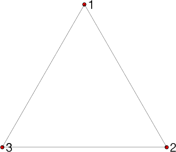
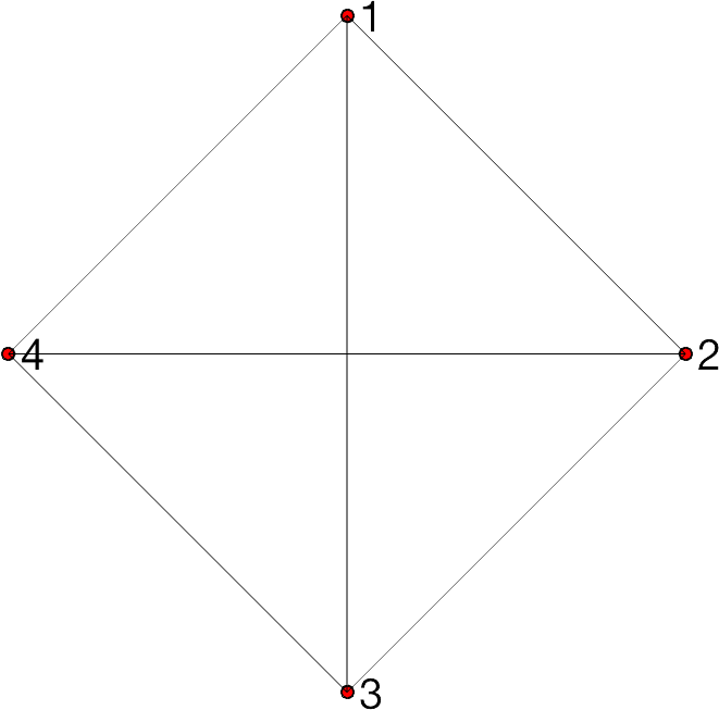
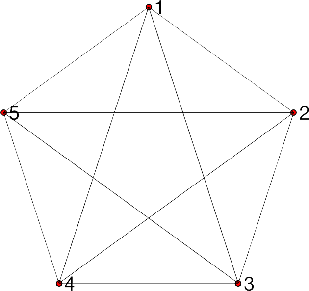
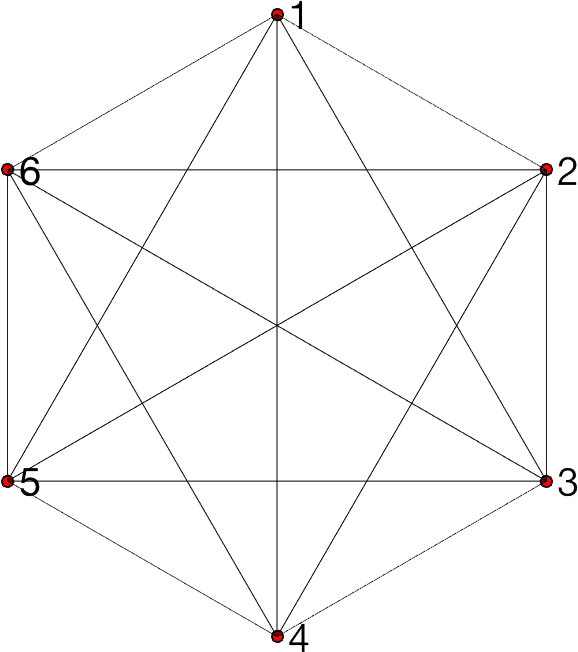
In the figure, we use $1,2,3...$ to represent different points’ index and each triangle is a covariant primitive. $L$ is the degree of the DAMI, which represents how many points has participated in the construction in total. Then the $primitives$ constructed with these points can be represented with $D_{S}(i,j,k)$, $D_{C}(l,m,n)$,…, and so on. Each combination of these triangles (with specified order) would be a $ShapeKernel$ or $ChannelKernel$ of $DAMI(3,3)$. There are limited numbers of triangles in the figure. And all combinations of $ShapeKernels$ and $ChannelKernels$ in each subfigure make up a Complete Set under the specific degree $L$ and specific order $K$. By the way, Complete Set with lower degree is included in that with higher degree. What we need to do is just specifying the $i,j,k$ and $l,m,n$ as the different indexes of points.

Here, we only consider $SpaceKernels$ and $ChannelKernels$ with order and degree both not greater than 4, which are corresponding to Figure 4(b). There are four triangles in total, $(1,2,3)$, $(1,2,4)$, $(1,3,4)$ and $(2,3,4)$. We use them to construct the $covariants$ and specify different orders which not bigger than 4. Then we can get different $DAMI(3,3)$ with different triangle combinations and different parameters $(P,Q,O_{S},O_{C})$. All of the combinations are listed in Table 1. It should be illuminated that some other combinations with other point indexes does not appear in the Table, because those combinations have the same topological structure with one in the table. One example is $D_{S}(2,3,4)D_{C}(2,3,4)$, which does not appear in table, but has the same topological structure with the first element in table, $D_{S}(1,2,3)D_{C}(1,2,3)$. These two will get the same invariant. So just one of them is listed in table. Finally, we get a Complete Set of all combinations with both degree and order not greater than 4. Each one has a specific $ID$ in Table 1. And $G$ in the first column of the table is used just to make our enumeration more convenient and orderliness.

Table 1: All combinations of degree and order not greater than 4, corresponding to Figure 4(b).

$G$	$ID$	Combination	$(P,Q,O_{S},O_{C})$
1	1	$D_{S}(1,2,3)D_{C}(1,2,3)$	(3,3,1,1)
1	2	$D_{S}(1,2,3)^{2}D_{C}(1,2,3)$	(3,3,2,1)
1	3	$D_{S}(1,2,3)D_{C}(1,2,3)^{2}$	(3,3,1,2)
1	4	$D_{S}(1,2,3)^{3}D_{C}(1,2,3)$	(3,3,3,1)
1	5	$D_{S}(1,2,3)D_{C}(1,2,3)^{3}$	(3,3,1,3)
1	6	$D_{S}(1,2,3)^{2}D_{C}(1,2,3)^{2}$	(3,3,2,2)
2	7	$D_{S}(1,2,3)D_{C}(1,2,4)$	(3,3,1,1)
2	8	$D_{S}(1,2,3)^{2}D_{C}(1,2,4)$	(3,3,2,1)
2	9	$D_{S}(1,2,3)D_{C}(1,2,4)^{2}$	(3,3,1,2)
2	10	$D_{S}(1,2,3)^{3}D_{C}(1,2,4)$	(3,3,3,1)
2	11	$D_{S}(1,2,3)D_{C}(1,2,4)^{3}$	(3,3,1,3)
2	12	$D_{S}(1,2,3)^{2}D_{C}(1,2,4)^{2}$	(3,3,2,2)
3	13	$D_{S}(1,2,3)D_{S}(1,2,4)D_{C}(1,2,3)$	(4,3,2,1)
3	14	$D_{S}(1,2,3)^{2}D_{S}(1,2,4)D_{C}(1,2,3)$	(4,3,3,1)
3	15	$D_{S}(1,2,3)D_{S}(1,2,4)^{2}D_{C}(1,2,3)$	(4,3,3,1)
3	16	$D_{S}(1,2,3)D_{S}(1,2,4)D_{C}(1,2,3)^{2}$	(4,3,2,2)
3	17	$D_{S}(1,2,3)D_{C}(1,2,3)D_{C}(1,2,4)$	(3,4,1,2)
3	18	$D_{S}(1,2,3)D_{C}(1,2,3)^{2}D_{C}(1,2,4)$	(3,4,1,3)
3	19	$D_{S}(1,2,3)D_{C}(1,2,3)D_{C}(1,2,4)^{2}$	(3,4,1,3)
3	20	$D_{S}(1,2,3)^{2}D_{C}(1,2,3)D_{C}(1,2,4)$	(3,4,2,2)
4	21	$D_{S}(1,2,3)D_{S}(1,3,4)D_{C}(1,2,4)$	(4,3,2,1)
4	22	$D_{S}(1,2,3)^{2}D_{S}(1,3,4)D_{C}(1,2,4)$	(4,3,3,1)
4	23	$D_{S}(1,2,3)D_{S}(1,3,4)D_{C}(1,2,4)^{2}$	(4,3,2,2)
4	24	$D_{S}(1,2,3)D_{C}(1,3,4)D_{C}(1,2,4)$	(3,4,1,2)
4	25	$D_{S}(1,2,3)D_{C}(1,3,4)^{2}D_{C}(1,2,4)$	(3,4,1,3)
4	26	$D_{S}(1,2,3)^{2}D_{C}(1,3,4)D_{C}(1,2,4)$	(3,4,2,2)
5	27	$D_{S}(1,2,3)D_{S}(1,2,4)D_{C}(1,3,4)D_{C}(2,3,4)$	(4,4,2,2)
5	28	$D_{S}(1,2,3)D_{S}(1,2,4)D_{S}(1,3,4)D_{C}(2,3,4)$	(4,4,3,1)
5	29	$D_{S}(1,2,3)D_{C}(1,2,4)D_{C}(1,3,4)D_{C}(2,3,4)$	(4,4,1,3)

4.2 Calculation

To calculate the $DAMI(3,3)$ in practice, we should expand the $DAMI(3,3)$ to the form of Moment. The basic geometric moment in 2D shape space is listed in Equation (35).

$$M_{pq}=\iint x^{p}y^{q}f(x,y)dxdy$$ (35)

And the central moment is replacing the origin with the centroid, as Equation (36):

$$U_{pq}=\iint(x-\overline{x})^{p}(y-\overline{y})^{q}f(x,y)dxdy$$ (36)

where $\overline{x}$ and $\overline{y}$ represent the center of the image in corresponding axis.

In 3D shape-color space, we define the $M(3,3)$ as Equation (37):

$$M(3,3)_{pqruvw}=\iiint x^{p}y^{q}z^{r}R(x,y,z)^{u}G(x,y,z)^{v}B(x,y,z)^{w}dxdydz$$ (37)

And the central moment is listed in Equation (4.2):

$$U(3,3)_{pqruvw}=\iiint (x-\overline{x})^{p}(y-\overline{y})^{q}(z-\overline{z})^{r}\cdot$$

$$(R-\overline{R})^{u}(G-\overline{G})^{v}(B-\overline{B})^{w}dxdydz$$ (38)

We can expand all the $DAMI(3,3)$ in the form of $U(3,3)$. By the way, some $DAMI(3,3)$ may expand to 0, such as 2,3,8,9,13,17,21,24, in Table 1. Several examples of expanded $DAMI(3,3)$ are listed in Equation (4.2-41). We use $ID$ listed in Table 1 to index the 29 $DAMI(3,3)$.

$$DA MI(3,3)(1)\_numerator=$$

$$6*u_{001001}*u_{010010}*u_{100100}-6*u_{001001}*u_{010100}*u_{100010}-$$

$$6*u_{001010}*u_{010001}*u_{100100}+6*u_{001010}*u_{010100}*u_{100001}+$$

$$6*u_{001100}*u_{010001}*u_{100010}-6*u_{001100}*u_{010010}*u_{100001}$$

$$DA MI(3,3)(1)\_denominator=$$

$$(-6*u_{000200}*{u_{000011}}^{2}+12*u_{000011}*u_{000101}*u_{000110}-$$

$$6*u_{000020}*{u_{000101}}^{2}-6*u_{000002}*{u_{000110}}^{2}+$$

$$6*u_{000002}*u_{000020}*u_{000200})^{1/2}*u_{000000}^{5/2}$$

$$DA MI(3,3)(1)=\frac{DAMI(3,3)(1)\_numerator}{DAMI(3,3)(1)\_denominator}$$ (39)

$$DA MI(3,3)(7)\_numerator=$$

$$2*u_{000001}*u_{001000}*u_{010010}*u_{100100}-2*u_{000001}*u_{001000}*$$

$$u_{010100}*u_{100010}-2*u_{000001}*u_{001010}*u_{010000}*u_{100100}+$$

$$2*u_{000001}*u_{001010}*u_{010100}*u_{100000}+2*u_{000001}*u_{001100}*$$

$$u_{010000}*u_{100010}-2*u_{000001}*u_{001100}*u_{010010}*u_{100000}-$$

$$2*u_{000010}*u_{001000}*u_{010001}*u_{100100}+2*u_{000010}*u_{001000}*$$

$$u_{010100}*u_{100001}+2*u_{000010}*u_{001001}*u_{010000}*u_{100100}-$$

$$2*u_{000010}*u_{001001}*u_{010100}*u_{100000}-2*u_{000010}*u_{001100}*$$

$$u_{010000}*u_{100001}+2*u_{000010}*u_{001100}*u_{010001}*u_{100000}+$$

$$2*u_{000100}*u_{001000}*u_{010001}*u_{100010}-2*u_{000100}*u_{001000}*$$

$$u_{010010}*u_{100001}-2*u_{000100}*u_{001001}*u_{010000}*u_{100010}+$$

$$2*u_{000100}*u_{001001}*u_{010010}*u_{100000}+2*u_{000100}*u_{001010}*$$

$$u_{010000}*u_{100001}-2*u_{000100}*u_{001010}*u_{010001}*u_{100000}$$

$$DA MI(3,3)(7)\_denominator=$$

$$(-6*u_{000200}*{u_{000011}}^{2}+12*u_{000011}*u_{000101}*u_{000110}-$$

$$6*u_{000020}*{u_{000101}}^{2}-6*u_{000002}*{u_{000110}}^{2}+$$

$$6*u_{000002}*u_{000020}*u_{000200})^{1/2}*u_{000000}^{5/2}$$

$$DA MI(3,3)(7)=\frac{DAMI(3,3)(7)\_numerator}{DAMI(3,3)(7)\_denominator}$$ (40)

$$DAMI(3,3)(2,3,8,9,13,17,21,24)=0$$ (41)

Considering the length, the others are not listed here.

5 Experiments for $DAMI(3,3)$

As listed in Table 1, except the 8 DAMIs that are expanded to 0, we get 21 usable DAMIs. In order to give a comprehensive analysis of these DAMIs, we conduct several experiments in this section. First, we select a typical object and design an experiment to evaluate the characteristics of DAMI for different types of transformations in Section 5.1. Then, we conduct experiments on some special objects with 1 or more symmetric planes in Section 5.2, which may affect the stability of some DAMIs. Through these cases, we can get the characteristics of each DAMI. Based on this analysis, we give some guidelines for selecting a high-order invariant kernels. Finally, we conduct a classification experiments for the dataset with dual-affine transformations in Section 5.3.

5.1 Invariance to different transformations

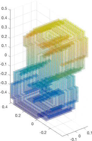
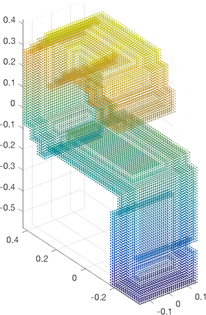
To evaluate the invariance of the $DAMI(3,3)$, we use one object from 3D-MNIST dataset, which is in 3D points cloud format. Then we assign color for every pixels based the $y$ coordination and generate one 3D color object, as shown in Figure 5(a). We transform it with some shape affine transformations, including translation, rotation, scaling, and affine, channel affine transformations and dual-affine transformations. Examples of the 3D color object and its transformed versions are shown in Figure 5.

(a) original

(b) translate

(c) rotation

(d) scaling

(e) affine

(f) color affine

(g) dual-Affine

Figure 5: A 3D color object of point cloud and its transformed versions.

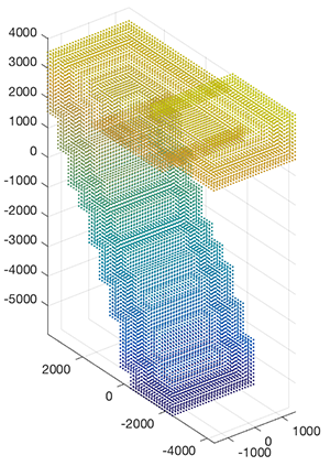
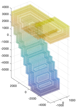
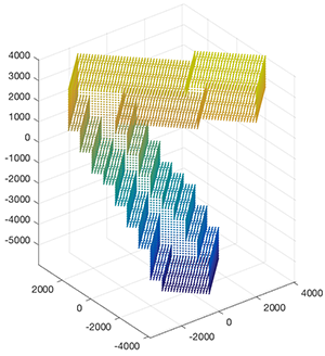
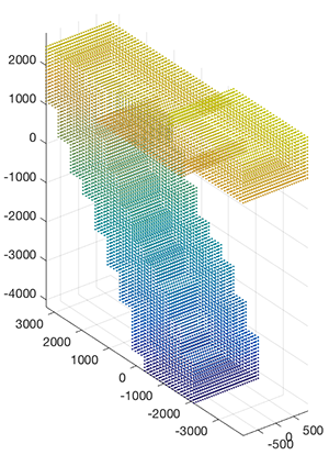
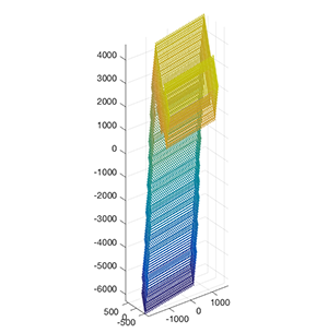
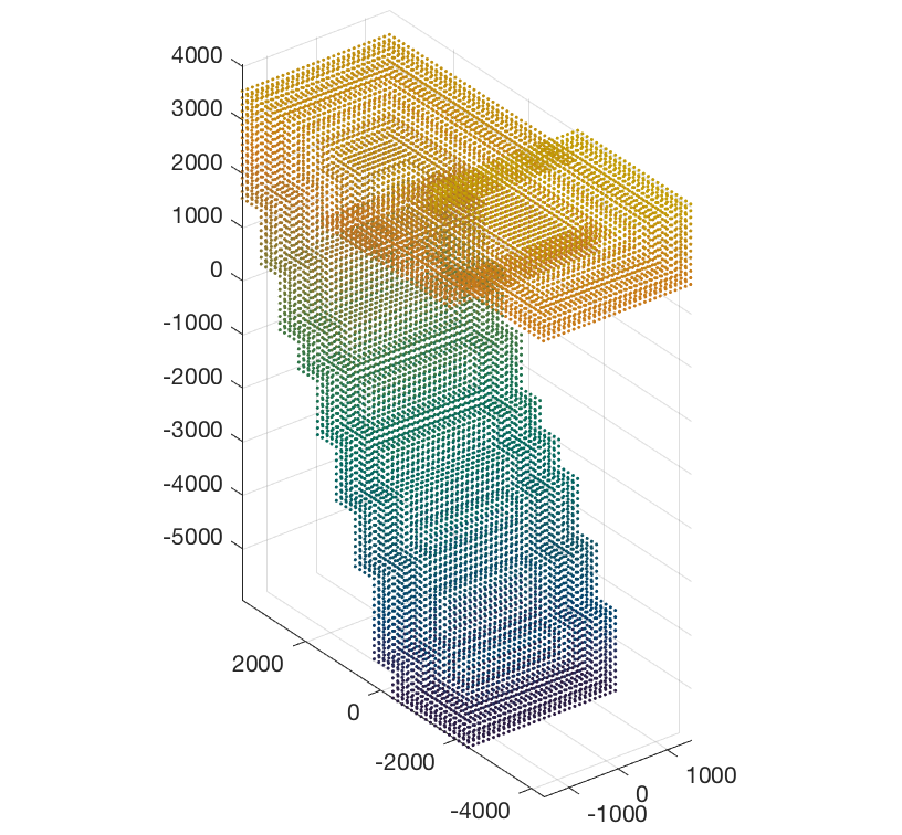
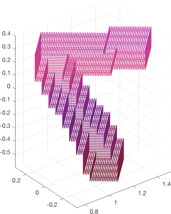
We calculate the 21 $DAMI(3,3)$ for these objects. To measure the stability of DAMIs, we calculate the coefficient of variation (CV), as Equation (42), for every DAMI to each type of the transformation. The results are listed in Table 2. The smaller of the CV is, the more robust of the invariant is. And 0 is the best.

$$c_{v}=\frac{\sigma}{\mu}$$ (42)

Table 2: The CVs of invariants for each type of transformation.

DAMI	translation	rotation	scaling	affine	color-affine	DAT	ALL
1	30.4598	1.9720	68.2011	1.9537	1.0516	2.4390	2.9668
4	49.0937	1.7006	4.1107	2.3175	0.5987	0.9042	5.4031
5	0.3933	1.5842	1.7944	2.0706	1.8723	1.0928	3.2553
6	0.0000	0.0000	0.0000	0.0000	0.0130	0.0130	0.0084
7	647.1033	1.2743	1.6939	1.9432	4.7739	2.0432	3.5687
10	1.0987	1.8283	2.0222	2.5839	2.8689	0.9317	2.9907
11	97.7044	1.3899	1.5922	1.9368	0.0407	0.9426	3.3357
12	0.0000	0.0000	0.0000	0.0000	0.0082	0.0082	0.0052
14	525.2069	1.2780	1.7163	0.7668	0.0169	0.9621	1.5313
15	8.1589	1.3549	2.0697	2.5449	0.6408	0.8617	16.5947
16	0.0000	0.0000	0.0000	0.0000	0.0765	0.0765	0.0550
18	1.0154	2.4479	1.3882	2.0443	1.1687	1.1411	3.8883
19	0.3031	1.6126	1.8729	2.0763	1.8352	1.0757	3.0969
20	0.0000	0.0000	0.0000	0.0000	1.5923	1.5923	4.8507
22	2.3639	1.8489	0.8868	2.5441	2.4992	1.3321	2.8626
23	0.0000	0.0000	0.0000	0.0000	0.1781	0.1781	0.1076
25	0.2547	1.7778	12.4229	2.0604	1.5818	2.1393	5.5918
26	0.0000	0.0000	0.0000	0.0000	0.0079	0.0079	0.0064
27	0.0000	0.0000	0.0000	0.0000	0.0516	0.0516	0.0316
28	3.3809	1.8488	0.5721	1.1201	1.5067	0.8754	5.1531
29	1.5408	1.2632	1.2428	2.1340	5.3576	1.2356	3.0848

From the results, we can see that not all $DAMI(3,3)$ are robust to all transformations. In general, invariants with $cv$ less than 1 are considered unstable. We can see that for all transformations of the object, there are 6 DAMIs robust, 6, 12, 16, 23, 26, 27. And No. 20 DAMI is only robust to shape affine transformations. We will conduct an in-depth analysis of the causes of the errors through experiments in the next subsection.

5.2 Guidelines for kernel selection

We analyzed the relationship between the $ShapeKernel$ and symmetric planes of the objects in shape space. In color space, the relationship is the same. However, the symmetry in color space rarely occurs on objects. Therefore, some invariants, with odd-order for some color kernels, are still robust to most objects. Another phenomenon we can see from Table 2 is that the 20th DAMI is not robust to color affine invariants. Its $ColorKernel$ is characterized by the fact that points (1, 2, 3) participate in both the shape $primitive$ and the color $primitive$ construction, and the sum of their orders is odd.

From the above experiments, we can conclude that the calculation of the central moment produces a tiny error for the central moment of all orders due to the tiny error in the calculation of the center of the object. When the object’s symmetric plane is exactly the coordinate plane, the odd moments will be symmetry too and the values of the moments will be close to 0. The absolute values of the error and the moment are on the same order of magnitude and this error will be manifested. In other cases, the magnitude of the error and the absolute value of the central moment differ greatly in magnitude, the error will be recessive, and the value of the central moment will not be affected. For some DAMIs, although the expression is not 0, the sum of the addend of the invariant is also close to 0, which will also causes this error to be manifested. In fact, the necessary and sufficient condition for the invariant to be stable for all objects is that when the invariant is finally expanded, there is one addend that all the central moments in it are even-order.

Considering the complexity of the actual application, we summarize the DAMI that can be used in different objects. First, when the objects in the dataset has no more than one symmetric plane, the available invariants are (6, 12, 16, 23, 26, 27). Second, when the objects in the dataset has three or more symmetrical planes, the available DAMIs are (6, 12, 26). Third, for very few cases where colors of the object are also symmetrical in color space, 26 may be unstable, and the available invariants are (6, 12). Fourth, for the case of objects with a single color, the numerator and denominator of DAMI are all 0. The DAMIs are not available. We can use the AMI only in shape space instead.

In order to be able to guide the derivation of higher-order stable invariants, we present some relationship between invariant kernels and invariant stability: First, A sufficient condition for the stability of DAMI is that the order of each shape kernel and color kernel is even. Second, a necessary condition for DAMI stability is that each point participating in the shape kernel and color kernel has an even number of participations. With these two guideline, we can derive DAMI in high-oder more easily.

5.3 Classification Experiment

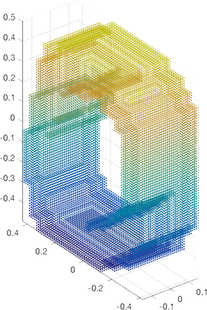
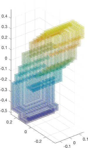
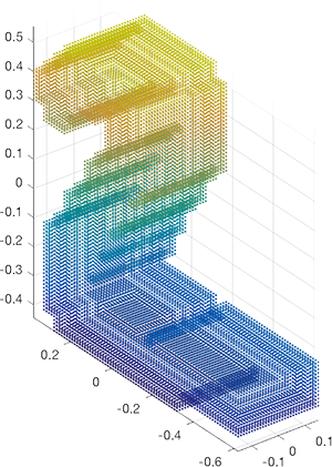
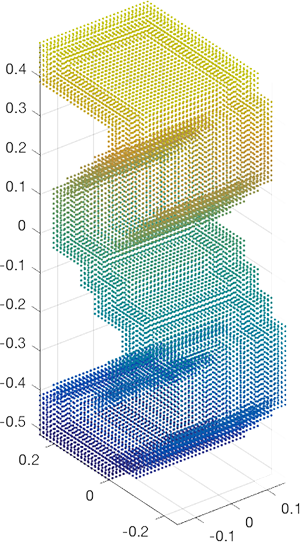
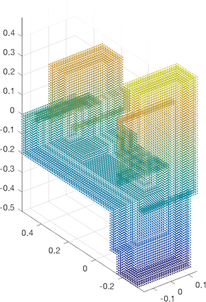
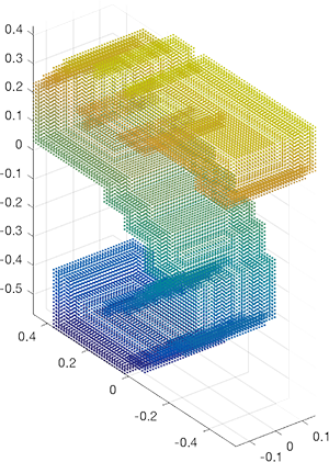
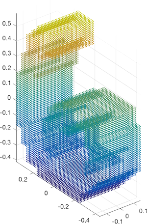
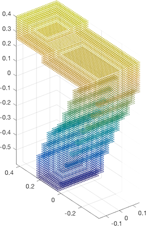
In order to evaluate the discriminability of invariants, we conduct classification experiments. We select 10 objects from 3D-MNIST dataset, which are shown in Figure 6. Then we conduct 13 DAT on each of them. Finally, we get a dataset with 140 objects of 10 classes. With the 6 $DAMI(3,3)$, (6, 12, 16, 23, 26, 27), we conduct 10-folds cross validation on the dataset with K-NearestNeighbor (KNN). The average accuracy is 100%. We can conclude that these six invariants have good discriminability.

(a) 0

(b) 1

(c) 2

(d) 3

(e) 4

(f) 5

(g) 6

(h) 7

(i) 8

(j) 9

Figure 6: 10 objects from 3D-MNIST dataset.

6 Conclusion

In this paper, we propose a general framework to derive Moment Invariants under Dual-Affine Transformation for objects in $M$-dimensional space with $N$ channels. With this framework, we can not only unify the invariants of objects with different dimensions into one framework, but also get the DAMI of objects with more complex formats. This framework integrate the DAMI of different data format into one framework, such as color image in 2D space with 3 channels, 2D vector field in 2D space with 2 channel, 3D color object in 3D shape with 3 channels and objects in higher dimensional space with multi-channels. This framework is consist with SCAMI in color images in Gong et al. (2017), and 2D vector field Kostková et al. (2018). We use the 3D color objects as an example and give out a complete set of $DAMI(3,3)$ with both order and degree not greater than 4. Then, we analyzed the root cause of the error in the moment invariant. At the same time, the invariant stability and the choice of the core in the construction process are given. This can play a very good role in the construction of higher moments. Through invariance analysis, we select six robust DAMIs, which are robust for the objects with no more than 1 symmetric plane. And we evaluated the discriminable of them with classification experiments. The results shown that the DAMI are robust for objects under DAT. We can use this framework to derive DAMI in higher-dimensional space with multiple channels.

References

- Alferez and Wang (1999) Alferez, R., Wang, Y.F., 1999. Geometric and illumination invariants for object recognition. IEEE Transactions on Pattern Analysis and Machine Intelligence 21, 505–536.
- Flusser and Suk (1993) Flusser, J., Suk, T., 1993. Pattern recognition by affine moment invariants. Pattern recognition 26, 167–174.
- Flusser and Suk (1994) Flusser, J., Suk, T., 1994. Affine moment invariants: a new tool for character recognition. Pattern recognition letters 15, 433–436.
- Funt and Finlayson (1995) Funt, B.V., Finlayson, G.D., 1995. Color constant color indexing. IEEE transactions on Pattern analysis and Machine Intelligence 17, 522–529.
- Geusebroek et al. (2001) Geusebroek, J.M., Van den Boomgaard, R., Smeulders, A.W.M., Geerts, H., 2001. Color invariance. IEEE Transactions on Pattern analysis and machine intelligence 23, 1338–1350.
- Gevers and Smeulders (1999) Gevers, T., Smeulders, A.W., 1999. Color-based object recognition. Pattern recognition 32, 453–464.
- Gong et al. (2017) Gong, M., Hao, Y., Mo, H., Li, H., 2017. Naturally combined shape-color moment invariants under affine transformations. Computer Vision and Image Understanding 162, 46–56.
- Gong et al. (2013) Gong, M., Li, H., Cao, W., 2013. Moment invariants to affine transformation of colours. Pattern Recognition Letters 34, 1240–1251.
- Hu (1962) Hu, M.K., 1962. Visual pattern recognition by moment invariants. IRE transactions on information theory 8, 179–187.
- Kostková and Flusser (2019) Kostková, J., Flusser, J., 2019. On the null-space of the shape-color moment invariants, in: International Conference on Computer Analysis of Images and Patterns, Springer. pp. 402–408.
- Kostková et al. (2018) Kostková, J., Suk, T., Flusser, J., 2018. Affine moment invariants of vector fields, in: 2018 25th IEEE International Conference on Image Processing (ICIP), IEEE. pp. 1338–1342.
- Kostkova et al. (2019) Kostkova, J., Suk, T., Flusser, J., 2019. Affine invariants of vector fields. IEEE Transactions on Pattern Analysis and Machine Intelligence doi:10.1109/TPAMI.2019.2951664.
- Li et al. (2009) Li, B., Xu, D., Xiong, W., Feng, S., 2009. Illumination-independent descriptors using color moment invariants. Optical Engineering 48, 027005.
- Li et al. (2017) Li, E., Huang, Y., Xu, D., Li, H., 2017. Shape dna: Basic generating functions for geometric moment invariants. arXiv preprint arXiv:1703.02242 .
- Li et al. (2018) Li, E., Mo, H., Xu, D., Li, H., 2018. Image projective invariants. IEEE transactions on pattern analysis and machine intelligence 41, 1144–1157.
- Lo and Don (1989) Lo, C.H., Don, H.S., 1989. 3-d moment forms: their construction and application to object identification and positioning. IEEE Transactions on Pattern Analysis and Machine Intelligence 11, 1053–1064.
- Mamistvalov (1998) Mamistvalov, A.G., 1998. N-dimensional moment invariants and conceptual mathematical theory of recognition n-dimensional solids. IEEE Transactions on pattern analysis and machine intelligence 20, 819–831.
- Mindru et al. (2004) Mindru, F., Tuytelaars, T., Van Gool, L., Moons, T., 2004. Moment invariants for recognition under changing viewpoint and illumination. Computer Vision and Image Understanding 94, 3–27.
- Mo et al. (2017) Mo, H., Li, S., Hao, Y., Li, H., 2017. Shape-color differential moment invariants under affine transforms, in: CCF Chinese Conference on Computer Vision, Springer. pp. 183–196.
- Mundy et al. (1992) Mundy, J.L., Zisserman, A., et al., 1992. Geometric invariance in computer vision. volume 92. MIT press Cambridge, MA.
- Novotni and Klein (2003) Novotni, M., Klein, R., 2003. 3d zernike descriptors for content based shape retrieval, in: Proceedings of the eighth ACM symposium on Solid modeling and applications, ACM. pp. 216–225.
- Rustamov et al. (2013) Rustamov, R.M., Ovsjanikov, M., Azencot, O., Ben-Chen, M., Chazal, F., Guibas, L., 2013. Map-based exploration of intrinsic shape differences and variability. ACM Transactions on Graphics (TOG) 32, 72.
- Schlemmer et al. (2007) Schlemmer, M., Heringer, M., Morr, F., Hotz, I., Hering-Bertram, M., Garth, C., Kollmann, W., Hamann, B., Hagen, H., 2007. Moment invariants for the analysis of 2d flow fields. IEEE Transactions on Visualization and Computer Graphics 13, 1743–1750.
- Stricker and Orengo (1995) Stricker, M.A., Orengo, M., 1995. Similarity of color images, in: Storage and retrieval for image and video databases III, International Society for Optics and Photonics. pp. 381–392.
- Suk and Flusser (2004a) Suk, T., Flusser, J., 2004a. Graph method for generating affine moment invariants, in: Proceedings of the 17th International Conference on Pattern Recognition, 2004. ICPR 2004., IEEE. pp. 192–195.
- Suk and Flusser (2004b) Suk, T., Flusser, J., 2004b. Projective moment invariants. IEEE Transactions on Pattern Analysis and Machine Intelligence 26, 1364–1367.
- Suk and Flusser (2009) Suk, T., Flusser, J., 2009. Affine moment invariants of color images, in: International Conference on Computer Analysis of Images and Patterns, Springer. pp. 334–341.
- Suk and Flusser (2011) Suk, T., Flusser, J., 2011. Affine moment invariants generated by graph method. Pattern Recognition 44, 2047–2056.
- Weiss (1988) Weiss, I., 1988. Projective invariants of shapes, in: Proceedings CVPR’88: The Computer Society Conference on Computer Vision and Pattern Recognition, IEEE. pp. 291–297.
- White (1973) White, J.H., 1973. A global invariant of conformal mappings in space. Proceedings of the American Mathematical Society 38, 162–164.
- Willmore (2000) Willmore, T.J., 2000. Surfaces in conformal geometry. Annals of Global Analysis and Geometry 18, 255–264.
- Xu and Li (2008) Xu, D., Li, H., 2008. Geometric moment invariants. Pattern recognition 41, 240–249.
- Zeng and Gu (2011) Zeng, W., Gu, X.D., 2011. Registration for 3d surfaces with large deformations using quasi-conformal curvature flow, in: CVPR 2011, IEEE. pp. 2457–2464.
- Zhang et al. (2018) Zhang, H., Mo, H., Hao, Y., Li, Q., Li, H., 2018. Differential and integral invariants under möbius transformation, in: Chinese Conference on Pattern Recognition and Computer Vision (PRCV), Springer. pp. 280–291.
- Zhang et al. (2017) Zhang, H., Mo, H., Hao, Y., Li, S., Li, H., 2017. Fast and efficient calculations of structural invariants of chirality. arXiv preprint arXiv:1711.05866 .
- Zhao and Chen (1997) Zhao, D., Chen, J., 1997. Affine curve moment invariants for shape recognition. Pattern recognition 30, 895–901.