Memory Effect or Cosmic String? Classifying Gravitational-Wave Bursts with Bayesian Inference

Abstract

In the event of a gravitational-wave burst candidate, a key question will be: which astrophysical signal hypothesis is most likely? Several different gravitational-wave transient sources can be modeled in the Fourier domain using a simple power law. This power-law model provides a reasonable approximation for gravitational-wave bursts from cosmic string cusps, cosmic string kinks, and the memory effect. Each of these sources is described using a different spectral index. In this work, we simulate interferometer strain data with injections of memory and other power-law bursts to demonstrate model selection in support of signal detection and for use in parameter estimation. We show how Bayesian inference can be used to measure the power-law spectral index, thereby distinguishing between different astrophysical scenarios. We propose a strategy for model selection of power-law burst signals for gravitational-wave candidates, and we aim to use this analysis to determine whether a specific candidate can be best described by a compact binary coalescence (CBC) signal or by some other interesting astrophysical mechanism.

I Introduction

The LIGO and Virgo Scientific Collaborations have cataloged eleven significant gravitational-wave signals in the first two observing runs  LIGOScientific:2018mvr and released 56 possible candidates in the third observing run to date, each of them originating from the coalescence of binary black holes or neutron stars. Considerable effort is also undertaken to search for gravitational-wave “bursts:” unmodeled (or minimally-modeled) transients. Bursting signals have been proposed for a variety of mechanisms including pulsar glitches  PhysRevLett.87.241101 , neutron star collapse Baiotti_2007 , core-collapse supernovae  Abbott:2016tdt , cosmic-string interactions  PhysRevD.64.064008 ; PhysRevD.73.105001 ; Key:2008tt , and gravitational-wave memory  PhysRevLett.118.181103 ; PhysRevD.45.520 . Previous searches for gravitational-wave bursts have included short-duration transients that arise from pulsar glitches and supernovae explosions  PhysRevD.100.024017 ; PhysRevD.95.042003 , long-duration transients such as those from fallback accretion  PhysRevD.99.104033 ; Abbott:2017muc , cosmic strings  Abbott:2017mem , binary black hole mergers  PhysRevLett.116.061102 ; PhysRevD.93.122004 , intermediate mass black hole mergers  PhysRevD.96.022001 , post-merger remnants from neutron star mergers  Abbott:2017dke , sub-solar mass binaries  Authors:2019qbw , eccentric binaries  strathprints70364 , those associated with magnetar bursts  Abbott:2019dxx , those associated with neutrino emission  PhysRevD.90.102002 , and those with electromagnetic counterparts  PhysRevD.93.122008 ; Abbott:2016cjt . Active pipelines that search for unmodeled burst transients include coherent WaveBurst (cWB)  Klimenko:2008fu and Omicron-LALInferenceBurst (oLIB)  PhysRevD.95.104046 . The possibility of an unexpected source is the most promising motivation for gravitational wave burst searches.

In the event of a gravitational-wave burst candidate, a key question will be: which astrophysical signal hypothesis is most likely? To answer this question, gravitational-wave candidates are first identified by detection pipelines such as cWB  Klimenko:2008fu , PyCBC  Usman:2015kfa , and GstLAL  Cannon:2011vi . In the process of identifying, these detection pipelines utilize techniques such as time-slides to determine if the data contains an astrophysical signal or a detector glitch by time shifting the detector data around the trigger time; see  Was:2009vh for further details. Once the noise hypothesis is ruled out by these pipelines, implying that there exists some astrophysical signal in the data, parameter estimation analyses such as Bilby  Ashton:2018jfp and LALInference  Veitch:2014wba begin by assuming Gaussian noise in the detectors and a CBC waveform approximant. In this paper, we are concerned with parameter estimation and model selection, and so we assume that a signal has already been detected by some other pipeline and that the noise is approximately Gaussian in the vicinity of the signal.

By introducing the power-law model to the set of all astrophysical signals that are analyzed, our method can be used to classify between power-law signals in addition to CBC signals for parameter estimation of gravitational-wave data. Furthermore, we extend our analysis to show how we rule out power-law burst sources for gravitational-wave candidates that have their astrophysical source in question. By combining our method with other burst classification techniques, it should be possible to construct a set of minimally-modeled bursts: supernovae bursts  Logue:2012zw ; PhysRevD.96.123013 , arbitrary power law bursts, an arbitrary superposition of wavelets  Cornish:2014kda ; Becsy:2016ofp , etc. Thus, our method contributes to the model selection for various astrophysical burst sources. By comparing the Bayesian evidence from the different models in the catalog, it will be possible to determine which catalog entry best describes the gravitational-wave burst candidate.

This paper is structured as follows: Section II describes the set of power-law signal models used in the analysis. Section  III reviews the fundamentals of Bayesian inference, establishes the prior distribution for each signal parameter, and lists the steps taken to simulate and analyze interferometer strain data. Section  IV presents results from a set of injection simulations with discussions on their implications.

II Signal models

We model signals with respect to phenomenological parameters, or signal characteristics, such that the dimensionality of each model remains low, ultimately reducing model complexity and improving statistical robustness. For example, rather than individually parameterizing the mass, distance, and inclination of an astrophysical system that emits memory, we just parameterize the “amplitude” and rise-time of a memory signal. In all models, we use $t_{A}$ to denote the arrival time of a given burst signal.

II.1 Memory

The non-linear memory effect, a prediction of general relativity, was first derived in  PhysRevLett.67.1486 . The memory effect is a linearly polarized, DC, gravitational-wave signal originating from an anisotropic gravitational-wave energy flux; see  Favata_2010 . Memory signals have a characteristic rise time $\tau$ proportional to the total mass of the astrophysical system  PhysRevD.45.520 . We model the time-domain waveform as,

$$h_{\text{m}}(t)=A_{\text{m}}\tanh\left(\frac{t-t_{A}}{\tau}\right).$$ (1)

Here $t$ is time, and $A_{\text{m}}$ is a parameter describing the memory amplitude. In the Fourier domain, this memory model has the analytic form,

$$\tilde{h}_{\text{m}}(f)=-i\pi A_{\text{m}}\tau e^{-2\pi ift_{A}}\left(\sinh(\pi^{2}\tau f)\right)^{-1}.$$ (2)

In the limit of $\tau\rightarrow 0$, corresponding to an astrophysical system with minimal mass, this memory model approaches $-iA_{\text{m}}e^{-2\pi ift_{A}}/\pi f$, a power-law signal with a negative spectral index of one or equivalently, a step-function in the time domain.

II.2 Cosmic String Interactions

It has been theorized that topological defects during a symmetry-breaking phase transition in the early Universe can give rise to one-dimensional strings that expand to cosmological scales and form cosmic string networks  PhysRevD.64.064008 . A network of cosmic strings can produce linearly polarized gravitational-wave bursts, arising from features such as cusps  Key:2008tt and kinks through string interactions. Cusps are parts of a cosmic string that move at relativistic speeds, their gravitational-wave emission is modelled by,

$$\tilde{h}_{\text{c}}(f)=A_{\text{c}}e^{-2\pi ift_{A}}f^{-4/3}\Theta\left(f_{h}-f\right).$$ (3)

Here and below, $f_{h}$ is a high frequency cutoff parameter that is inversely proportional to the cube of the beaming angle, which is defined as the angle between the line of sight and emission cone axis; see  Key:2008tt for further details. Kink signals are sourced from discontinuities in the string’s tangent vector, with their resulting waveform being modelled as,

$$\tilde{h}_{\text{k}}(f)=A_{\text{k}}e^{-2\pi ift_{A}}f^{-5/3}\Theta\left(f_{h}-f\right).$$ (4)

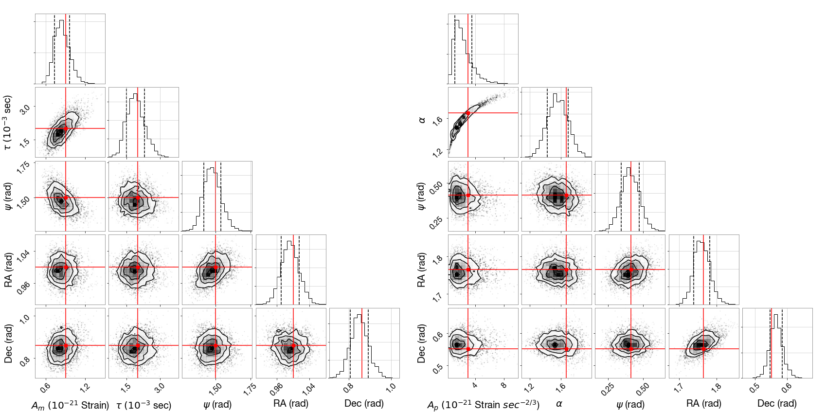
FIG. 1: Marginalized posterior distributions for each signal parameter of the memory model (left), with signal/noise log Bayes factor $\ln(\text{BF})$ = 68.8 and an arbitrary power-law model (right), with $\alpha=$ 5/3, and with signal/noise $\ln(\text{BF})$ = 60.8. The red lines show the values of the injected parameters and the dotted lines in each one-dimensional posterior distribution represent one standard deviation credible intervals. The contour levels of the two-dimensional posterior distributions are $0.5,1.0,1.5,\text{and}~{}2$ standard deviations. These plots show how well we recover signal parameters of a given astrophysical model.

II.3 Arbitrary Power Law

Inspired by the morphological similarity between memory and string waveforms we propose to search for a general power-law signal, which might capture a range of scale-invariant phenomena that emit gravitational waves. We assume linear polarization and define a general power-law model,

$$\tilde{h}_{\text{p}}(f)=A_{\text{p}}e^{-2\pi ift_{A}}f^{-\alpha},$$ (5)

where $\alpha$ is the power-law spectral index.

III Method

III.1 Bayesian Inference

We use Bayesian inference to estimate parameters and calculate the significance of each signal model given observed data. We denote the complex, frequency-domain strain data to be $d$ and a given frequency-domain waveform model $\mu(\theta)$ as a function of signal parameters $\theta$. We denote the prior distribution on signal parameters as $\pi(\theta)$. We then construct the posterior probability distribution $p(\theta|d)$ using Bayes’ theorem

$$p\left(\theta|d\right)=\frac{\mathcal{L}\left(d|\theta\right)\pi(\theta)}{\mathcal{Z}}.$$ (6)

We employ a Gaussian likelihood function,

$$\ln\mathcal{L}\left(d|\theta\right)=-\frac{1}{2}\Big{[}\sum_{j}\frac{|d_{j}-\mu_{j}(\theta)|^{2}}{\sigma_{j}^{2}}+2\ln\left(2\pi\sigma_{j}^{2}\right)\Big{]}.$$ (7)

The summation in the likelihood function is taken over $j$ frequency bins and $\sigma_{j}$ is the noise amplitude spectral density of the detector in the $j^{th}$ frequency bin. We assume Gaussian noise for the remainder of our analysis. The evidence is calculated by

$$\mathcal{Z}=\int\mathcal{L}\left(d|\theta\right)\pi(\theta)d\theta.$$ (8)

Given a pair of signal models, $M_{1}$ and $M_{2}$ with the ratio of the prior odds set to unity, we compare models to noise $N$, and models to each other by computing Bayes factors $\text{BF}^{M_{1}}_{N}=\mathcal{Z}_{M_{1}}/{\mathcal{Z}_{N}}$ (signal versus noise) and $\text{BF}^{M_{1}}_{M_{2}}=\mathcal{Z}_{M_{1}}/\mathcal{Z}_{M_{2}}$ (model one versus model two). Following convention Jeffreys61 , we here consider $\ln(\text{BF})>8$ to be strong evidence for a particular hypothesis.

III.2 Prior Distributions

We establish the choice of prior distribution for each parameter present in each of the signal models. The bounds of our prior distributions are chosen to match the observing band of the detectors. For example, $\pi(\tau)$ and $\pi(f_{h})$ are uniformly distributed with bounds from $0.5-50\,\mathrm{ms}$ and $20-2000\,\mathrm{Hz}$, respectively. We chose a log uniform prior for the amplitude of the first cosmic string, memory, and power law detection to reflect our belief that any order or magnitude is as likely as any other order of magnitude. We chose the prior for the spectral index in Eq. 5, $\pi(\alpha)$, to be uniform on the interval $[0,2]$, which includes the cosmic string models without the frequency cutoff as a subset of the power-law model. We use standard priors for extrinsic parameters such as polarization angle and sky location. We explicitly marginalize over the arrival time and we can numerically reconstruct its posterior distribution in post-processing; see, e.g., Thrane:2018qnx .

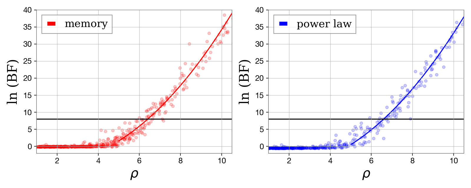
FIG. 2: Signal/noise Bayes factor versus matched-filter signal-to-noise ratio $\rho$ for simulated memory (left), and power-law events (right). The signal model is chosen to match the injection. The horizontal axis is the matched filter signal-to-noise ratio. The individual dots represent the Bayes factors for a particular injection. We fit a quadratic function, shown by the solid curves, to each panel. The horizontal black line corresponds to a Bayes factor of $\ln\text{BF}=8$. These plots quantify how loud a memory or power-law burst signal has to be for the signal hypothesis to be significantly larger than the noise hypothesis.

III.3 Procedure

We outline the steps taken to simulate interferometer strain data and to run our Bayesian inference analysis on a given signal injection. We set the total duration of the data segment to be 4 seconds at a sampling rate of 4096 Hz. All signals are injected with $t_{A}=2\,\mathrm{s}.$ We assume a three-detector network consisting of two Advanced LIGO detectors and one Advanced Virgo detector operating at design sensitivity Aasi:2013wya . We generate Gaussian noise and inject a power-law signal with a randomly chosen set of injection parameters. We set the minimum and maximum frequency of our detectors to be $[20\,\mathrm{Hz},2000\,\mathrm{Hz}]$, corresponding to the most sensitive region of our detectors. We define the total joint matched-filter signal-to-noise ratio (SNR) and inner-product to be

$$\rho =\frac{\langle d,\mu\rangle_{\text{tot}}}{\langle\mu,\mu\rangle_{\text{tot}}^{1/2}},$$ (9)

$$\big{\langle}a,b\big{\rangle}_{\text{tot}} \equiv 4\Delta f\sum_{k}\sum_{j}\mathcal{R}\left(\frac{a_{j,k}^{*}b_{j,k}}{\sigma^{2}_{j,k}}\right).$$ (10)

Here, $\Delta f$ is the frequency resolution and $k$ is an index for the detector. We carry out inference using the nested-sampling algorithm “dynesty” with 500 live points 2019arXiv190402180S . We use the Bayesian inference software package Bilby  Ashton:2018jfp to perform our analysis.

IV Simulations

IV.1 Parameter Estimation

To infer the properties of a gravitational-wave burst event, we calculate the posterior distributions for each parameter in a given signal model. We show the one-dimensional and two-dimensional posterior distributions for an injection of a memory and cosmic string kink signal in Fig. 1, quantifying how well we recover a set of injected parameters. The posterior distribution for the spectral index in the power-law model differentiates between various astrophysical burst scenarios.

IV.2 Signal Detection

We calculate how loud a memory and power-law event must be for the respective signal hypothesis to be significantly more likely than the noise hypothesis. We show results from injection simulations of memory and power-law signals in Fig. 2.

IV.3 Model Selection

Given that the noise hypothesis is ruled out by one of the detection pipelines, we can also differentiate between various astrophysical burst scenarios by calculating the model versus model Bayes factor for a pair of signal hypotheses. Suppose we were to detect a cosmic string cusp signal, how do we establish that it is not a memory or kink burst? To demonstrate how we use the Bayes factor in such a scenario, we simulate a set of cosmic string cusp signal events with $f_{h}=1000\,\mathrm{Hz}$ and perform a search for a cusp, kink, memory and power-law burst for each individual simulation. By incrementally increasing the amplitude of the cusp signal throughout our injections, while keeping all other parameters fixed , we observe how our confidence increases with the loudness of the injected cusp signal, shown in Fig. 3.

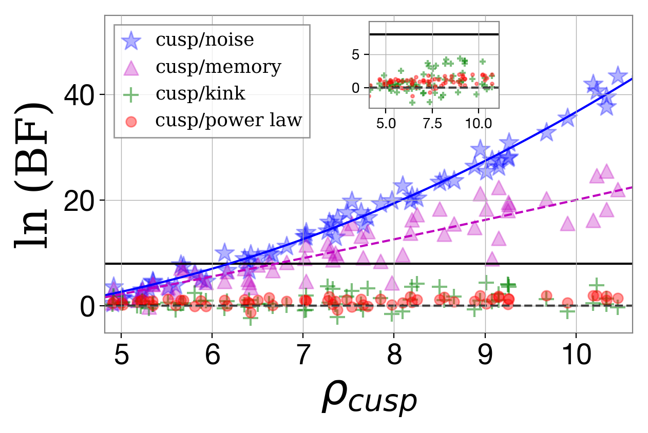
FIG. 3: In these simulations, the individual points represent the calculated Bayes factors when comparing the cusp signal model to noise (blue stars), memory (magenta triangles), kink (green plus) and power-law (red circles) models. Quadratic fits comparing cusp to noise (solid blue) and cusp to memory (dashed magenta) are shown. The horizontal black solid line corresponds to $\ln(\text{BF})=8$ and the dashed line to $\ln(\text{BF})=0$. This plot establishes how well we can distinguish cosmic string bursts from other power-law bursts.

When comparing the cusp to memory at a signal-to-noise ratio of $\sim 7$, the cusp hypothesis is more significant than the memory hypothesis. The cusp/power law Bayes factor remains between $\ln(\text{BF})=0$ and $\ln(\text{BF})=8$ in Fig. 3, which implies it is difficult to significantly distinguish between a cosmic string signal with a large frequency cutoff and an arbitrary power-law signal in this signal-to-noise ratio interval.

IV.4 Extension to Binary Black Hole Mergers

We now expand our set of bursting signals to include a CBC signal and calculate the model-to-model Bayes factors for a CBC signal and some other power-law burst. For example, in the event of a detection of a massive binary black hole merger, one with large component spins, or one with a large mass ratio, the merger waveform may look qualitatively different than the “chirping” waveforms observed thus far  LIGOScientific:2018mvr . In the case of a massive binary black hole merger, the CBC signal can look similar to a cosmic string cusp or kink signal, shown in Fig. 4. In such situations, it will be natural to ask whether or not a particular gravitational-wave candidate originated from a compact binary coalescence or a cosmic string interaction.

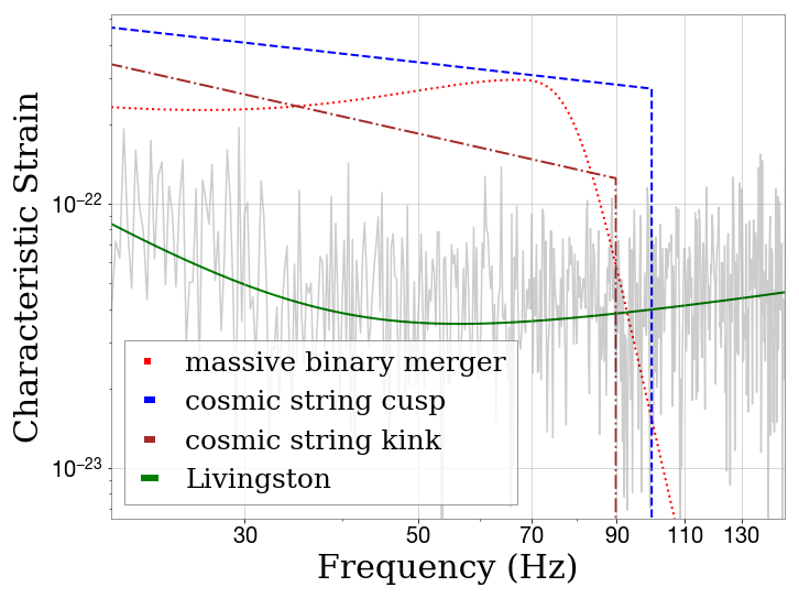
FIG. 4: Frequency domain plot showing the characteristic strain of the noise amplitude spectral density of the Livingston detector (solid green curve) and a noise realization (gray region), a massive binary merger with $M_{\text{tot}}=250\,\mathrm{M_{\odot}}$ (dashed blue curve), a cosmic string cusp (dotted red curve), and a cosmic string kink (dotted dashed brown curve). When injected into a three-detector network, all signals have similar signal-to-noise ratios.

As an example of model selection between CBC and cosmic string signals, we simulate an equal-mass massive binary black hole merger signal with total mass $M_{\text{tot}}=250\,\mathrm{M_{\odot}}$, at signal-to-noise $\rho=14.5$, using the IMRPhenomPv2 waveforms  PhysRevD.93.044006 ; PhysRevD.93.044007 . This results in a signal that is in-band for only the merger-ringdown portion of the coalescence. We perform a search for a binary black hole, a cosmic string cusp (Eq. 3), and a cosmic string kink (Eq. 4) signal. We calculate the following Bayes factors: $\ln(\text{BF}^{BBH}_{cusp})=86.9~{}\text{and}~{}\ln(\text{BF}^{BBH}_{kink})=86.7$. Given the magnitude of these Bayes factors, the black hole signal hypothesis is significantly more likely than either of the cosmic string burst signals. In this case, we are able to rule out cosmic strings as the astrophysical origin of the burst event.

V Summary and Outlook

In this paper, we present a unified framework for classifying gravitational-wave burst signals from memory, cosmic strings, and other bursts that are well approximated by a power law in the Fourier domain. We establish how the arbitrary power-law models can be used to search for signals that cover a wide range of astrophysical burst scenarios. Using simulations, we estimate the signal parameters of a gravitational-wave burst, identify astrophysical signals from interferometer noise, and characterize between power-law bursts by measuring their spectral index.

In testing our classification method we have assumed Gaussian noise. In reality, ground-based interferometer detector noise is populated by glitches, power lines, seismic activity, and other transient noise sources. In future work, we will investigate how to handle the non-Gaussian nature of noise   Ashton:2019wvo , for example, using techniques such as the Bayes Coherence Ratio defined in  Isi:2018vst .

Our signal models are of low dimensionality, especially when compared to the large parameter space of CBC signals. Therefore, it takes only a few minutes to analyze a few seconds of data using a single core processor. We aim to use this analysis to determine whether a gravitational-wave candidate can be best described by a CBC signal or by some other interesting astrophysical mechanism.

Acknowledgements

We thank Colm Talbot, Rory Smith, and Gregory Ashton who provided helpful discussion of parameter estimation and Bayesian statistics. The authors gratefully acknowledge the support from the University of Florida through the National Science Foundation (NSF) grants PHY-1205512, PHY-1460803, PHY-1607323 and the Australian Research Council (ARC) grants CE170100004, FT150100281, FT160100112, and DP180103155. Computing resources of the LIGO Data Grid at the Caltech Institute of Technology were used for this paper. We thank the 2018 Australia-Americas PhD Research Internship Program, which was supported by the Australian Government Department of Education and Training through the Australian International Education: Enabling Growth and Innovation (EGI) project fund, for further information, please visit www.internationaleducation.gov.au.’ This work was also supported by Monash University in providing resources and accommodation. This is LIGO document No: LIGO-P1900297.

References

- [1] B. P. Abbott et al. GWTC-1: A Gravitational-Wave Transient Catalog of Compact Binary Mergers Observed by LIGO and Virgo during the First and Second Observing Runs. Phys. Rev., X9(3):031040, 2019.
- [2] N. Andersson and G. L. Comer. Probing neutron-star superfluidity with gravitational-wave data. Phys. Rev. Lett., 87:241101, Nov 2001.
- [3] L. Baiotti, I. Hawke, and L. Rezzolla. On the gravitational radiation from the collapse of neutron stars to rotating black holes. Classical and Quantum Gravity, 24(12):S187–S206, may 2007.
- [4] B. P. Abbott et al. A First Targeted Search for Gravitational-Wave Bursts from Core-Collapse Supernovae in Data of First-Generation Laser Interferometer Detectors. Phys. Rev., D94(10):102001, 2016.
- [5] T. Damour and A. Vilenkin. Gravitational wave bursts from cusps and kinks on cosmic strings. Phys. Rev. D, 64:064008, Aug 2001.
- [6] X. Siemens, J. Creighton, I. Maor, S. R. Majumder, K. Cannon, and J. Read. Gravitational wave bursts from cosmic (super)strings: Quantitative analysis and constraints. Phys. Rev. D, 73:105001, May 2006.
- [7] J. S. Key and N. J. Cornish. Characterizing the Gravitational Wave Signature from Cosmic String Cusps. Phys. Rev., D79:043014, 2009.
- [8] L. O. McNeill, E. Thrane, and P. D. Lasky. Detecting gravitational wave memory without parent signals. Phys. Rev. Lett., 118:181103, May 2017.
- [9] K. S. Thorne. Gravitational-wave bursts with memory: The christodoulou effect. Phys. Rev. D, 45:520–524, Jan 1992.
- [10] B. P. Abbott et al. All-sky search for short gravitational-wave bursts in the second advanced ligo and advanced virgo run. Phys. Rev. D, 100:024017, Jul 2019.
- [11] B. P. Abbott et al. All-sky search for short gravitational-wave bursts in the first advanced ligo run. Phys. Rev. D, 95:042003, Feb 2017.
- [12] B. P. Abbott et al. All-sky search for long-duration gravitational-wave transients in the second advanced ligo observing run. Phys. Rev. D, 99:104033, May 2019.
- [13] B. P. Abbott et al. All-sky search for long-duration gravitational wave transients in the first Advanced LIGO observing run. Class. Quant. Grav., 35(6):065009, 2018.
- [14] B. P. Abbott et al. Constraints on cosmic strings using data from the first Advanced LIGO observing run. Phys. Rev., D97(10):102002, 2018.
- [15] B. P. Abbott et al. Observation of gravitational waves from a binary black hole merger. Phys. Rev. Lett., 116:061102, Feb 2016.
- [16] B. P. Abbott et al. Observing gravitational-wave transient gw150914 with minimal assumptions. Phys. Rev. D, 93:122004, Jun 2016.
- [17] B. P. Abbott et al. Search for intermediate mass black hole binaries in the first observing run of advanced ligo. Phys. Rev. D, 96:022001, Jul 2017.
- [18] B. P. Abbott et al. Search for Post-merger Gravitational Waves from the Remnant of the Binary Neutron Star Merger GW170817. Astrophys. J., 851(1):L16, 2017.
- [19] B. P. Abbott et al. Search for sub-solar mass ultracompact binaries in Advanced LIGO’s second observing run. Phys. Rev. Lett., 123(16):161102, 2019.
- [20] B. P. Abbott et al. Search for eccentric binary black hole mergers with advanced ligo and advanced virgo during their first and second observing runs. Astrophysical Journal, 883(2), September 2019.
- [21] B. P. Abbott et al. Search for Transient Gravitational-wave Signals Associated with Magnetar Bursts during Advanced LIGO’s Second Observing Run. Astrophys. J., 874(2):163, 2019.
- [22] M. G. Aartsen et al. Multimessenger search for sources of gravitational waves and high-energy neutrinos: Initial results for ligo-virgo and icecube. Phys. Rev. D, 90:102002, Nov 2014.
- [23] B. P. Abbott et al. Search for transient gravitational waves in coincidence with short-duration radio transients during 2007–2013. Phys. Rev. D, 93:122008, Jun 2016.
- [24] B. P. Abbott et al. Search for Gravitational Waves Associated with Gamma-Ray Bursts During the First Advanced LIGO Observing Run and Implications for the Origin of GRB 150906B. Astrophys. J., 841(2):89, 2017.
- [25] S. Klimenko, I. Yakushin, A. Mercer, and G. Mitselmakher. Coherent method for detection of gravitational wave bursts. Class. Quant. Grav., 25:114029, 2008.
- [26] R. Lynch, S. Vitale, R. Essick, E. Katsavounidis, and F. Robinet. Information-theoretic approach to the gravitational-wave burst detection problem. Phys. Rev. D, 95:104046, May 2017.
- [27] S. A. Usman et al. The PyCBC search for gravitational waves from compact binary coalescence. Class. Quant. Grav., 33(21):215004, 2016.
- [28] K. Cannon et al. Toward Early-Warning Detection of Gravitational Waves from Compact Binary Coalescence. Astrophys. J., 748:136, 2012.
- [29] M. Was, M. Bizouard, V. Brisson, F. Cavalier, and Miltiadis others Vavoulidis. On the background estimation by time slides in a network of gravitational wave detectors. Class. Quant. Grav., 27:015005, 2010.
- [30] G. Ashton et al. BILBY: A user-friendly Bayesian inference library for gravitational-wave astronomy. Astrophys. J. Suppl., 241(2):27, 2019.
- [31] J. Veitch et al. Parameter estimation for compact binaries with ground-based gravitational-wave observations using the LALInference software library. Phys. Rev., D91(4):042003, 2015.
- [32] J. Logue, C. D. Ott, I. S. Heng, P. Kalmus, and J. H. C. Scargill. Inferring Core-Collapse Supernova Physics with Gravitational Waves. Phys. Rev., D86:044023, 2012.
- [33] J. Powell, M. Szczepanczyk, and I. S. Heng. Inferring the core-collapse supernova explosion mechanism with three-dimensional gravitational-wave simulations. Phys. Rev. D, 96:123013, Dec 2017.
- [34] N. J. Cornish and T. B. Littenberg. BayesWave: Bayesian Inference for Gravitational Wave Bursts and Instrument Glitches. Class. Quant. Grav., 32(13):135012, 2015.
- [35] B. Bécsy, P. Raffai, N. J. Cornish, R. Essick, J. Kanner, E. Katsavounidis, T. B. Littenberg, M. Millhouse, and S. Vitale. Parameter estimation for gravitational-wave bursts with the BayesWave pipeline. Astrophys. J., 839(1):15, 2017.
- [36] D. Christodoulou. Nonlinear nature of gravitation and gravitational-wave experiments. Phys. Rev. Lett., 67:1486–1489, Sep 1991.
- [37] M. Favata. The gravitational-wave memory effect. Classical and Quantum Gravity, 27(8):084036, apr 2010.
- [38] H. Jeffreys. Theory of Probability. Oxford, Oxford, England, third edition, 1961.
- [39] E. Thrane and C. Talbot. An introduction to Bayesian inference in gravitational-wave astronomy: parameter estimation, model selection, and hierarchical models. Publ. Astron. Soc. Austral., 36:10, 2019.
- [40] B. P. Abbott et al. Prospects for Observing and Localizing Gravitational-Wave Transients with Advanced LIGO, Advanced Virgo and KAGRA. Living Rev. Rel., 21(1):3, 2018.
- [41] J. Speagle. dynesty: A Dynamic Nested Sampling Package for Estimating Bayesian Posteriors and Evidences. arXiv e-prints, page arXiv:1904.02180, Apr 2019.
- [42] S. Husa, S. Khan, M. Hannam, M. Pürrer, F. Ohme, X. J. Forteza, and A. Bohé. Frequency-domain gravitational waves from nonprecessing black-hole binaries. i. new numerical waveforms and anatomy of the signal. Phys. Rev. D, 93:044006, Feb 2016.
- [43] S. Khan, S. Husa, M. Hannam, F. Ohme, M. Pürrer, X. J. Forteza, and A. Bohé. Frequency-domain gravitational waves from nonprecessing black-hole binaries. ii. a phenomenological model for the advanced detector era. Phys. Rev. D, 93:044007, Feb 2016.
- [44] G. Ashton, E. Thrane, and R. J. E. Smith. Gravitational wave detection without boot straps: a Bayesian approach. Phys. Rev., D100(12):123018, 2019.
- [45] M. Isi, R. Smith, S. Vitale, T. J. Massinger, J. Kanner, and A. Vajpeyi. Enhancing confidence in the detection of gravitational waves from compact binaries using signal coherence. Phys. Rev., D98(4):042007, 2018.