33email: {shivam.kalra,m7adnan}@uwaterloo.ca gwtaylor@uoquelph.ca tizhoosh@uwaterloo.ca
Learning Permutation Invariant Representations using Memory Networks
Abstract
††∗Authors have equal contribution.Many real world tasks such as classification of digital histopathological images and 3D object detection involve learning from a set of instances. In these cases, only a group of instances or a set, collectively, contains meaningful information and therefore only the sets have labels, and not individual data instances. In this work, we present a permutation invariant neural network called Memory-based Exchangeable Model (MEM) for learning universal set functions. The MEM model consists of memory units which embed an input sequence to high-level features enabling it to learn inter-dependencies among instances through a self-attention mechanism. We evaluated the learning ability of MEM on various toy datasets, point cloud classification, and classification of whole slide images (WSIs) into two subtypes of lung cancer—Lung Adenocarcinoma, and Lung Squamous Cell Carcinoma. We systematically extracted patches from WSIs of lung, downloaded from The Cancer Genome Atlas (TCGA) dataset, the largest public repository of WSIs, achieving a competitive accuracy of 84.84% for classification of two sub-types of lung cancer. The results on other datasets are promising as well, and demonstrate the efficacy of our model.
Keywords:
Permutation Invariant Models, Multi Instance Learning, Whole Slide Image Classification, Medical Images1 Introduction
Deep artificial neural networks have achieved impressive performance for representation learning tasks. The majority of these deep architectures take a single instance as an input. Recurrent Neural Networks (RNNs) are a popular approach to learn representations from sequential ordered instances. However, the lack of permutation invariance renders RNNs ineffective for exchangeable or unordered sequences. We often need to learn representations of unordered sequential data, or exchangeable sequences in many practical scenarios such as Multiple Instance Learning (MIL). In the MIL scenario, a label is associated with a set, instead of a single data instance. One of the application of MIL is classification of high resolution histopathology images, called whole slide images (WSIs). Each WSI is a gigapixel image with size 50,000 50,000 pixels. The labels are generally associated with the entire WSI instead of patch, region, or pixel level. MIL algorithms can be used to learn representations of these WSIs by disassembling them into multiple representative patches [14, 1, 15].
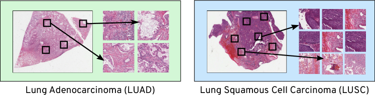
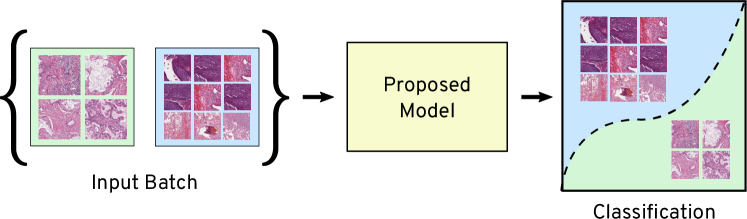
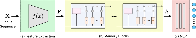
In this paper, we propose a novel architecture for exchangeable sequences incorporating attention over the instances to learn inter-dependencies. We use the results from Deep Sets [39] to construct a permutation invariant model for learning set representations. Our main contribution is a sequence-to-sequence permutation invariant layer called Memory Block. The proposed model uses a series of connected memory block layers, to model complex dependencies within an input set using a self attention mechanism. We validate our model using a toy datasets and two real-world applications. The real world applications include, i) point cloud classification, and ii) classification of WSI into two sub-type of lung cancers—Lung Adenocarcinoma (LUAD)/ Lung Squamous Cell Carcinoma (LUSC) (see Figure 1).
2 Related Work
In statistics, exchangeability has been long studied. de Finetti studied exchangeable random variables and showed that sequence of infinite exchangeable random variables can be factorised to independent and identically distributed mixtures conditioned on some parameter . Bayesian sets [8] introduced a method to model exchangeable sequences of binary random variables by analytically computing the integrals in de Finetti’s theorem. Orbanz et. al. [22] used de Finetti’s theorem for Bayesian modelling of graphs, matrices, and other data that can be modeled by random structures. Considerable work has also been done on partially exchangeable random variables [2].
Symmetry in neural networks was first proposed by Shawe et al. [26] under the name Symmetry Network. They proposed that invariance can be achieved by weight-preserving automorphisms of a neural network. Ravanbaksh et al. proposed a similar method for equivariance network through parameter sharing [24]. Bloem Reddy et al. [4] studied the concept of symmetry and exchangeability for neural networks in detail and established similarity between functional and probabilistic symmetry, and obtained generative functional representations of joint and conditional probability distributions that are invariant or equivariant under the action of a compact group. Zhou et. al. [41] proposed treating instances in a set as non identical and independent samples for multi instance problem.
Most of the work published in recent years have focused on ordered sets. Vinyals
et. al. introduced Order Matter: Sequence to Sequence for Sets in 2016 to learn
a sequence to sequence mapping. Many related models and key contributions have
been proposed that uses the idea of external memories like
RNNSearch [3], Memory
Networks [34, 32] and Neural Turing
Machines [10]. Recent interest in exchangeable models was
developed due to their application in MIL. Deep Symmetry
Networks [7] used kernel-based interpolation to tractably tie
parameters and pool over symmetry spaces of any dimension. Deep
Sets [39] by Zaheer et al. proposed a permutation invariant
model. They proved that any pooling operation (mean, sum, max or similar) on
individual features is a universal approximator for any set function. They also
showed that any permutation invariant model follows de Finetti’s theorem.Work
has also been done on learning point cloud classification which is an example of
MIL problem. Deep Learning with Sets and Point Cloud [23]
used parameter sharing to get a equivariant layer. Another important paper on
exchangeable model is Set Transformer. Set
Transformer [19] by Lee et al. used results
from Zaheer et al. [39] and proposed a
Transformer [32] inspired permutation invariant neural
network. The Set Transformer uses attention mechanisms to attend to inputs in
order to invoke activation. Instead of using averaging over instances like in
Deep Sets, the Set Transformer uses a parametric aggregating function pool which
can adapt to the problem at hand. Another way to handle exchangeable data is to
modify RNNs to operate on exchangeable data. BRUNO [18] is
a model for exchangeable data and makes use of deep features learned from
observations so as to model complex data types such as images. To achieve this,
they constructed a bijective mapping between random variables in
the observation space and features , and explicitly define an
exchangeable model for the sequences . Deep Amortized
Clustering [20] proposed using Set Transformers to cluster sets of
points with only few forward passes. Deep Set Prediction
Networks [40] introduced an interesting approach to predict sets
from a feature vector which is in contrast to predicting an output using sets.
MIL for Histopathology Image Analysis. Exchangeable models are useful for histopathological images analysis as ground-truth labeling is expensive and labels are available at WSI instead of at the pixel level. A small pathology lab may process 10,000 WSIs/year, producing a vast amount of data, presenting a unique opportunity for MIL methods. Dismantling a WSI into smaller patches is a common practice; these patches can be used for MIL. The authors in [12] used attention-based pooling to infer important patches for cancer classification. A large amount of partially labeled data in histopathology can be used to discover hidden patterns of clinical importance [17]. Authors in [28] used MIL for breast cancer classification. A permutation invariant operator introduced by [31, 30] was applied to pathology images. Recently, graph CNNs have been successfully used for representation learning of WSIs [1]. These compact and robust representations of WSIs can be further used for various clinical applications such as image-based search to make well-informed diagnostic decisions [15, 14].
3 Background
This section explains the general concepts of exchangeability, its relation to
de Finetti’s theorem, and briefly discusses Memory Networks.
Exchangeable Sequence. A sequence of random variables
is exchangeable if the joint probability distribution
does not change on permutation of the elements in a set. Mathematically, if
for a permutation
function , then the sequence is exchangeable.
Exchangeable Models. A model is said to be exchangeable if the output of the model is invariant to the permutation of its inputs. Exchangeability implies that the information provided by each instance is independent of the order in which they are presented. Exchangeable models can be of two types depending on the application: i) permutation invariant, and ii) permutation equivariant.
A model represented by a function where is a set, is said to be permutation equivariant if permutation of input instances permutes the output labels with the same permutation . Mathematically, a permutation-equivariant model is represented as,
| (1) |
Similarly, a function is permutation invariant if permutation of input instances does not change the output of the model. Mathematically,
| (2) |
Deep Sets [39] incorporate a permutation-invariant model to
learn arbitrary set functions by pooling in a latent space. The authors further
showed that any pooling operation such as averaging and max on individual
instances of a set can be used as a universal approximator for any arbitrary set
function. The authors proved the following two results about permutation invariant models.
Theorem 1. A function operating on a set
,…, having elements from a countable universe, is a valid set
function, i.e., invariant to the permutation of instances in , if it can be
decomposed to , for any function
and .
Theorem 2. Assume the elements are from a compact set in
, i.e., possibly uncountable, and the set size is fixed to .
Then any continuous function operating on a set , i.e., which is permutation invariant to the elements in
can be approximated arbitrarily close in the form of .
The Theorem 1 is linked to de Finetti’s theorem, which states that a random infinitely exchangeable sequence can be factorised into mixture densities conditioned on some parameter which captures the underlying generative process i.e.
| (3) |
Memory Networks. The idea of using an external memory for relational learning tasks was introduced by Weston et al. [34]. Later, an end-to-end trainable model was proposed by Sukhbaatar et al. [29]. Memory networks enable learning of dependencies among instances of a set by providing an explicit memory representation for each instance in the sequence. The idea of self attention is popularized by [32], these models are known as transformers, widely used in NLP applications. The proposed MEM model uses the self-attention (similar to transformers) within memory vectors, aggregated using a pooling operation (weighted averaging) to form a permutation-invariant representation (based on Theorems 1 and 2). The next section explains it in details.
4 Proposed Approach
This section discusses the motivations, components, and offers an analysis of the proposed Memory-based Exchangeable Model (MEM) capable of learning permutation invariant representation of sets and unordered sequences.
4.1 Motivation
In order to learn an efficient representation for a set of instances, it is important to focus on instances which are “important” for a given task at hand, i.e., we need to attend to specific instances more than other instances. We therefore use the memory network to learn an attention mapping for each instance. Memory networks are conventionally used for NLP for mapping questions posted in natural language to an answer [34, 29]. We exploit the idea of having memories which can learn key features shared by one or more instances. Through these key features, the model can learn inter-dependencies using transformer style self-attention mechanism. As inter-dependencies are learnt, a set can be condensed into a compact vector such that a MLP can be used for a classification or regression learning.
4.2 Model Components
MEM is composed of four sequentially connected units: i) a feature extraction model, ii) memory units, iii) memory blocks, and iv) fully connected layers to predict the output.
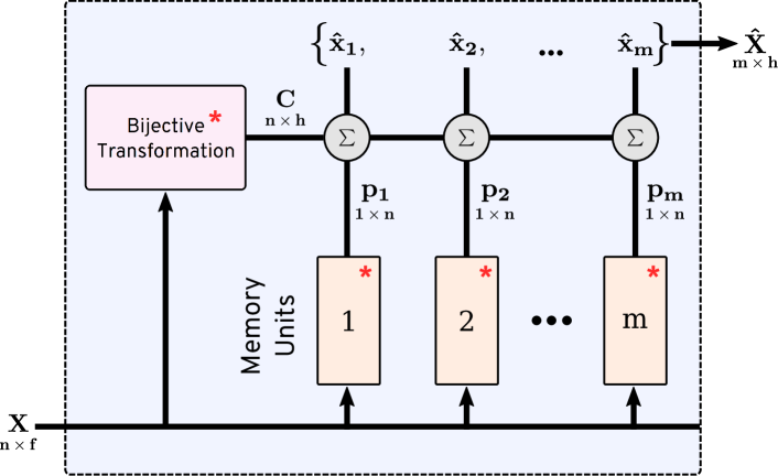
A memory block is the main component of MEM and learns a permutation
invariant representation of a given input sequence. Multiple memory blocks can
be stacked together for modeling complex relationships and dependencies in
exchangeable data. The memory block is made of memory units and a bijective
transformation unit shown in Figure 2
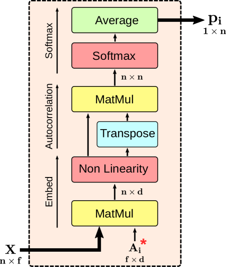
Memory Unit. A memory unit transforms a given input sequence to an attention vector. The higher attention value represents the higher “importance” of the corresponding element of the input sequence. Essentially, it captures the relationships among different elements of the input. Multiple memory units enable the memory block to capture many complex dependencies and relationships among the elements. Each memory unit consists of an embedding matrix that transforms a -dimensional input vector to a -dimensional memory vector , as follows:
where is some non-linearity. The memory vectors are stacked to form a matrix of the shape . The relative degree of correlations among the memory vectors are computed using cross-correlation followed by a column-wise softmax and then taking a row-wise average, as follows:
| (4) |
The is the final output vector () from the memory unit , as shown in Figure 2. The purpose of memory unit is to embed feature vectors into another space that
could correspond to a distinct “attribute” or “characteristic” of
instances. The cross correlation or the calculated attention vector represents
the instances which are highly suggestive of those “attributes” or
“characteristic”. We do not normalize memory vectors as magnitude of these
vectors may play an important role during the cross correlation.
Memory Block. A memory block is a sequence-to-sequence model,
i.e., it transforms a given input sequence to another
representative sequence . The output
sequence is invariant to the element-wise permutations of the input sequence. A
memory block contains number of memory units. In a memory block, each memory
unit takes a sequential data as an input and generates an attention vector.
These attention vectors are subsequently used to compute the final output
sequence. The schematic diagram of a memory block is shown
in 2(a).
The final output sequence of a memory block is computed as a weighted sum of with the probability distributions from all the memory units where is a bijective transformation of learned using an autoencoder. Each memory block has its own autoencoder model to learn the bijective mapping. The element of the output sequence is computed as matrix multiplication of and , as follows:
where, is the output of memory unit given by (4).
The bijective transformation from enables equivariant correspondence between the elements of the two sequences & , and maps two different elements in the input sequence to different elements in the output sequence. It must be noted that bijective transformation is permutation equivariant not invariant. The reconstruction maintains one-to-one mapping between and . The final output sequence from a memory block is permutation invariant as it uses matrix multiplication between (attention) and .
4.3 Model Architecture
-
1.
Each element of a given input sequence is passed through a feature extraction model to produce a sequence of feature vectors .
-
2.
The feature sequence is then passed through a memory block to obtain another sequence which is a permutation-invariant representation of the input sequence. The number of elements in the sequence depends on the number of memory unit in the memory block layer.
-
3.
Multiple memory blocks can be stacked in series. The output from the last memory block is either vectorized or pooled, which is subsequently passed to a MLP layer for classification or regression.
4.4 Analysis
This section discusses the mathematical properties of our model. We use theorems from
Deep Sets [39] to prove that our model is permutation invariant
and universal approximator for arbitrary set functions.
Property 1. Memory units are permutation equivariant.
Consider an input sequence . Since, for each memory unit,
By Equation (1), is permutation equivariant and thus in (4) is permutation equivariant. Finally, the attention vector is calculated by averaging all rows, therefore the final output of memory unit is permutation equivariant.
Property 2. Memory Blocks are permutation invariant.
A memory block layer consisting of m memory units generates a sequence where can be written as:
Since both and are permutation equivariant,
therefore, , which is calculated by
matrix multiplication of and , is permutation invariant.
5 Experiments
We performed two series of experiments comparing MEM against the simple pooling
operations proposed by Deep Sets [39]. In the first series of
experiments, we established the learning ability of the proposed model using toy
datasets. For the second series, we used two real-world dataset, i)
classification of subtypes of lung cancer against the largest public dataset of
histopathology whole slide images (WSIs) [33], and ii) 3-D
object classification using Point Cloud Dataset [36].
Model Comparison. We compared the performance of MEM against Deep Sets [39]. We use same the feature extractor for both Deep Sets and MEM, and experimented with different choices of pooling operations—max, mean, dot product, and sum. MEM also has a special pooling “”, which is a memory block with a single memory unit in the last hidden layer. Therefore, we tested 9 different models for each experiment—five configurations of our model, and four configurations of Deep Sets. We tried to achieve the best performance by varying the hyper-parameters for each of the configuration of both MEM and Deep Sets. We found that MEM had higher learning capacity, therefore higher number of parameters resulted in better accuracy for MEM but not necessarily for Deep Set. We denote the common feature extractor as FF and Deep Sets as DS in the discussion below. The other approaches that are compared have been appropriately cited.
5.1 Toy Datasets
| Sum of Even | Prime | Counting Unique | Maximum of | Gaussian | ||||
| Methods | Digits | Sum | Images | Set | Clustering | |||
| Accuracy | MAE | Accuracy | Accuracy | MAE | Accuracy | MAE | NLL | |
| FF + MEM + MB1 (ours) | 0.9367 0.0016 | 0.2516 0.0105 | 0.9438 0.0043 | 0.7108 0.0084 | 0.3931 0.0080 | 0.9326 0.0036 | 0.1449 0.0068 | 1.348 |
| FF + MEM + Mean (ours) | 0.9355 0.0015 | 0.2437 0.0087 | 0.7208 0.0217 | 0.4264 0.0062 | 0.9525 0.0109 | 0.9445 0.0035 | 0.1073 0.0067 | 1.523 |
| FF + MEM + Max (ours) | 0.9431 0.0020 | 0.2295 0.0098 | 0.9361 0.0060 | 0.6888 0.0066 | 0.4140 0.0079 | 0.9498 0.0022 | 0.1086 0.0060 | 1.388 |
| FF + MEM + Dotprod (ours) | 0.8411 0.0045 | 0.3932 0.0065 | 0.9450 0.0086 | 0.7284 0.0055 | 0.3664 0.0037 | 0.9517 0.0041 | 0.0999 0.0097 | 1.363 |
| FF + MEM + Sum (ours) | 0.9353 0.0022 | 0.2739 0.0081 | 0.6652 0.0389 | 0.3138 0.0094 | 1.3696 0.0151 | 0.9430 0.0031 | 0.1318 0.0058 | 1.611 |
| FF + Mean (DS) | 0.9159 0.0019 | 0.2958 0.0049 | 0.5280 0.0078 | 0.3140 0.0071 | 1.2169 0.0136 | 0.3223 0.0075 | 1.0029 0.0155 | 2.182 |
| FF + Max (DS) | 0.6291 0.0047 | 1.3292 0.0211 | 0.9257 0.0033 | 0.7088 0.0060 | 0.3933 0.0059 | 0.9585 0.0012 | 0.0742 0.0032 | 1.608 |
| FF + Dotprod (DS) | 0.1503 0.0015 | 1.8015 0.0016 | 0.9224 0.0028 | 0.7254 0.0063 | 0.3726 0.0054 | 0.9548 0.0017 | 0.1355 0.0027 | 8.538 |
| FF + Sum (DS) | 0.6333 0.0043 | 0.5763 0.0069 | 0.5264 0.0050 | 0.2982 0.0042 | 1.3415 0.0169 | 0.3344 0.0038 | 0.9645 0.0111 | 12.05 |
To demonstrate the advantage of MEM over simple pooling operations, we consider
four toy problems, involving regression and classification over sets. We
constructed these toy datasets using the MNIST dataset.
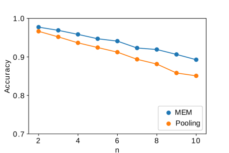
Sum of Even Digits. Sum of even digits is a regression problem over the set of
images containing handwritten digits from MNIST. For a given set of images , the goal is to find the sum of all even digits. We used the
Mean Absolute Error (MAE). We split the MNIST dataset into 70-30%
training, and testing data-sets, respectively. We sampled 100,000 sets of 2 to
10 images from the training data. For testing, we sampled 10,000
sets of images containing number of images per set where .
Figure 4 shows the performance of MEM against simple pooling
operations with respect to the number of images in the set.
Prime Sum. Prime Sum is a classification problem over a set of MNIST
images. A set is labeled positive if it contains any two digits such that their
sum is a prime number. We constructed the dataset by randomly sampling five
images from the MNIST dataset. We
constructed the training data with 20,000 sets randomly sampled from the
training data of MNIST. For testing, we randomly sampled 5,000 sets from the
testing data of MNIST. The
results are reported in the second column of Table 1 that
shows the robustness of memory block.
Maximum of a Set. Maximum of a set is a regression problem to predict the
highest digit present in a set of images from MNIST. We constructed a set of
five images by randomly selecting samples from MNIST dataset. The label for each
set is the largest number present in the set. For example, images of is labeled as . We constructed 20,000 training sets and for
testing we randomly sampled 5,000. The detailed comparison of accuracy and MAE between
different models is given in the second last column of
Table 1. We found that FF+Max learns the identity mapping
and thus results in a very high accuracy. In all the training sessions, we
consistently obtained the training accuracy of 100% for the FF+Max configuration,
whereas MEM generalizes better than the Deep Sets.
Counting Unique Images. Counting unique images is a regression problem over a set. This task involves counting unique objects in a set of images from fashion MNIST dataset [37]. We constructed the training data by selecting a set, as follows:
-
1.
Let n be the number of total images and u be the number of unique image in the set.
-
2.
Randomly select an integer between 2 and 10.
-
3.
Randomly select another integer between 1 and .
-
4.
Select number of unique objects from fashion-MNIST training data.
-
5.
Then add - number of randomly selected objects from the previous step.
The task is to count unique objects in a given set. The results are shown in the third column
of Table 1.
Amortized Gaussian Clustering. Amortized Gaussian clustering is a regression problem that involves estimating the parameters of a population of Mixture of Gaussian (MoG). Similar to Set Transformer [19], we test our model’s ability to learn parameters of a Gaussian Mixture with components such that the likelihood of the observed samples is maximum. This is in contrast to the EM algorithm which updates parameters of the mixture recursively until the stopping criterion is satisfied. Instead, we use MEM to directly predict parameters of a MoG i.e. . For simplicity we sample from MoG with only four components. The Generative process for each training dataset is as follows
-
1.
Mean of each Gaussian is selected from a uniform distribution i.e. .
-
2.
Select a cluster for each instance in the set, i.e.,
-
3.
Generate data from an univariate Gaussian .
We created a dataset of 20,000 sets each consisting of 500 points sampled from different MoGs. Results in Table 1 show that MEM is significantly better than Deep Sets.
5.2 Real World Datasets
To show the robustness and scalability of the model for the real-world problems,
we have validated MEM on two larger datasets. Firstly, we tested our model on a
point cloud dataset for predicting the object type from the set of 3D
coordinates. Secondly, we used the largest public repository of histopathology
images (TCGA) [33] to differentiate between two main
sub-types of lung cancer. Without any significant effort in extracting
histologically relevant features and fine-tuning, we achieved a remarkable
accuracy of 84.84% on 5-fold validation.
Point Cloud Classification. We evaluated MEM on a more complex classification task using ModelNet40 [36] point cloud dataset. The dataset consists of 40 different objects or classes embedded in a three dimensional space as points. We produce point-clouds with 100 points (x, y, z-coordinates) each from the mesh representation of objects using the point-cloud library’s sampling routine [25]111We obtained the training and test datasets from Zaheer et al. [39]. We compare the performance against various other models reported in Table 2. We experimented with different configurations of our model and found that FF+MB1 works best for 100 points cloud classification. We achieves the classification accuracy of 85.21% using 100 points. Our model performs better than Deep Sets and Set Transformer for the same number of instances, showing the effectiveness of having attention from memories.
| Configuration | Instance Size | Accuracy |
| 3DShapeNet [36] | 303 | 0.77 |
| Deep set [39] | 100 | 0.8200 |
| VoxNet [21] | 322 | 0.8310 |
| 3D GAN [35] | 643 | 0.833 |
| Set Transformer [19] | 100 | 0.8454 |
| Set Transformer [19] | 1000 | 0.8915 |
| Deep set [39] | 5000 | 0.9 |
| MVCNN [27] | 164 164 12 | 0.901 |
| Set Transformer [19] | 5000 | 0.9040 |
| VRN Ensemble [5] | 323 | 0.9554 |
| FF + MEM + MB1 (Ours) | 100 | 0.8521 |
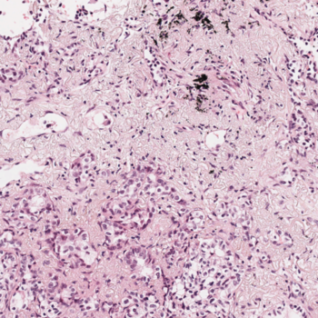
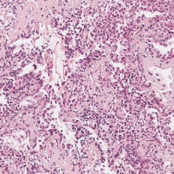
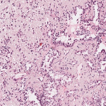
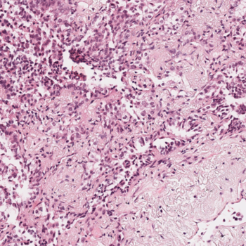
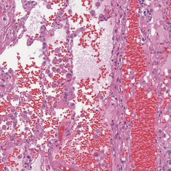
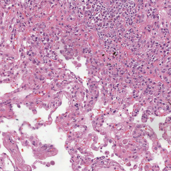
Lung Cancer Subtype Classification. Lung Adenocarcinoma (LUAD) and Lung Squamous Cell Carcinoma (LUSC) are two main types of non-small cell lung cancer (NSCLC) that account for 65-70% of all lung cancers [9]. Classifying patients accurately is important for prognosis and therapy decisions. Automated classification of these two main subtypes of NSCLC is a crucial step to build computerized decision support and triaging systems. We present a two-staged method to differentiate LUAD and LUSC for whole slide images, short WSIs, that are very large images. Firstly, we implement a method to systematically sample patches/tiles from WSIs. Next, we extract image features from these patches using Densenet [11]. We then use MEM to learn the representation of a set of patches for each WSI.
To the best of our knowledge, this is the first ever study conducted on all the lung cancer slides in TCGA dataset (comprising of 2 TB of data consisting of 2.5 million patches of size 10001000 pixels). All research works in literature use a subset of the WSIs with their own test-train split instead of cross validation, making it difficult to compare against them. However, we have achieved greater than or similar to all existing research works without utilizing any expert’s opinions (pathologists) or domain-specific techniques. We used 2,580 WSIs from TCGA public repository [33] with 1,249, and 1,331 slides for LUAD and LUSC, respectively. We process each WSI as follows.
-
1.
Tissue Extraction. Every WSI contains a bright background that generally contains irrelevant (non-tissue) pixel information. We removed non-tissue regions using color thresholds.
-
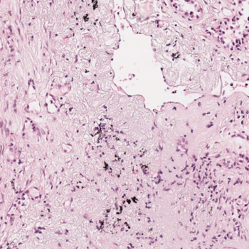
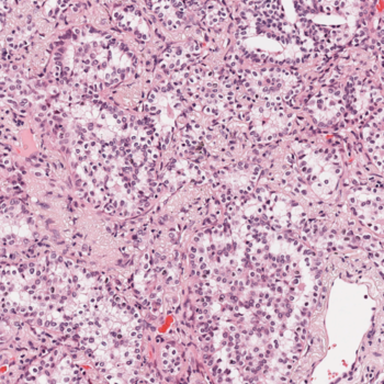
2.
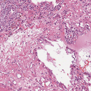
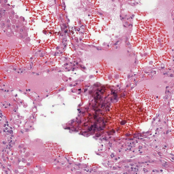
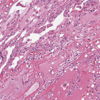
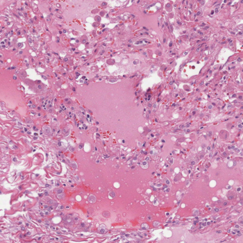
Selecting Representative Patches. Segmented tissue is then divided into patches. All the patches are then grouped into a pre-set number of categories (classes) via a clustering method. A 10% of all clustered patches are uniformly randomly selected distributed within each class to assemble representative patches. Six of these representative patches for each class (LUAD and LUSC) is shown in Figure 5.
-
3.
Feature Set. A set of features for each WSI is created by converting its representative patches into image features. We use DenseNet [11] as the feature extraction model. There are a different number of feature vectors for each WSI.
| Methods | Accuracy |
| Coudray et al. [6] | 0.85 |
| Jabber et al. [13] | 0.8333 |
| Khosravi et al. [16] | 0.83 |
| Yu et al. [38] | 0.75 |
| FF + MEM + Sum (ours) | 0.8484 0.0210 |
| FF + MEM + Mean (ours) | 0.8465 0.0225 |
| FF + MEM + MB1 (ours) | 0.8457 0.0219 |
| FF + MEM + Dotprod (ours) | 0.6345 0.0739 |
| FF + sum (DS) | 0.5159 0.0120 |
| FF + mean (DS) | 0.7777 0.0273 |
| FF + dotprod (DS) | 0.4112 0.0121 |
The results are shown in Table 3. We achieved the maximum accuracy of 84.84% with FF + MEM + Sum configuration. It is difficult to compare our approach against other approaches in literature due to non-standardization of the dataset. Coudray et al. [6] used the TCGA dataset with around 1,634 slides to classify LUAD and LUSC. They achieved AUC of 0.947 using patches at 20. We achieved a similar AUC of for one of the folds and average AUC of . In fact, without any training they achieved the similar accuracy as our model (around 85%). It is important to note that we did not do any fine-tuning or utilize any form of input from an expert/pathologist. Instead, we extracted diverse patches and let the model learn to differentiate between two sub-types by “attending” relevant ones. Another study by Jaber et al. [13] uses cell density maps, achieving an accuracy of 83.33% and AUC of 0.9068. However, they used much smaller portion of the TCGA, i.e., 338 TCGA diagnostic WSIs (164 LUAD and 174 LUSC) were used to train, and 150 (71 LUAD and 79 LUSC).
6 Conclusions
In this paper, we introduced a Memory-based Exchangeable Model (MEM) for learning permutation invariant representations. The proposed method uses attention mechanisms over “memories” (higher order features) for modelling complicated interactions among elements of a set. Typically for MIL, instances are treated as independently and identically distributed. However, instances are rarely independent in real tasks, and we overcome this limitation using an “attention” mechanism in memory units, that exploits relations among instances. We also prove that the MEM is permutation invariant. We achieved good performance on all problems that require exploiting instance relationships. Our model scales well on real world problems as well, achieving an accuracy score of 84.84% on classifying lung cancer sub-types on the largest public repository of histopathology images.
References
- [1] Adnan, M., Kalra, S., Tizhoosh, H.R.: Representation Learning of Histopathology Images Using Graph Neural Networks p. 8
- [2] Aldous, D.J.: Representations for partially exchangeable arrays of random variables. Journal of Multivariate Analysis 11(4), 581–598 (1981)
- [3] Bahdanau, D., Cho, K., Bengio, Y.: Neural machine translation by jointly learning to align and translate. arXiv preprint arXiv:1409.0473 (2014)
- [4] Bloem-Reddy, B., Teh, Y.W.: Probabilistic symmetry and invariant neural networks. arXiv preprint arXiv:1901.06082 (2019)
- [5] Brock, A., Lim, T., Ritchie, J.M., Weston, N.: Generative and Discriminative Voxel Modeling with Convolutional Neural Networks http://arxiv.org/abs/1608.04236
- [6] Coudray, N., Ocampo, P.S., Sakellaropoulos, T., Narula, N., Snuderl, M., Fenyö, D., Moreira, A.L., Razavian, N., Tsirigos, A.: Classification and mutation prediction from non–small cell lung cancer histopathology images using deep learning. Nature medicine 24(10), 1559 (2018)
- [7] Gens, R., Domingos, P.M.: Deep symmetry networks. In: Advances in neural information processing systems. pp. 2537–2545 (2014)
- [8] Ghahramani, Z., Heller, K.A.: Bayesian sets. In: Advances in neural information processing systems. pp. 435–442 (2006)
- [9] Graham, S., Shaban, M., Qaiser, T., Koohbanani, N.A., Khurram, S.A., Rajpoot, N.: Classification of lung cancer histology images using patch-level summary statistics. In: Medical Imaging 2018: Digital Pathology. vol. 10581, p. 1058119. International Society for Optics and Photonics (2018)
- [10] Graves, A., Wayne, G., Danihelka, I.: Neural turing machines. arXiv preprint arXiv:1410.5401 (2014)
- [11] Huang, G., Liu, Z., Van Der Maaten, L., Weinberger, K.Q.: Densely connected convolutional networks. In: Proceedings of the IEEE conference on computer vision and pattern recognition. pp. 4700–4708 (2017)
- [12] Ilse, M., Tomczak, J.M., Welling, M.: Chapter 22 - Deep multiple instance learning for digital histopathology. In: Zhou, S.K., Rueckert, D., Fichtinger, G. (eds.) Handbook of Medical Image Computing and Computer Assisted Intervention, pp. 521–546. Academic Press. https://doi.org/10.1016/B978-0-12-816176-0.00027-2
- [13] Jaber, M.I., Beziaeva, L., Szeto, C.W., Elshimali, J., Rabizadeh, S., Song, B.: Automated adeno/squamous-cell nsclc classification from diagnostic slide images: A deep-learning framework utilizing cell-density maps (2019)
- [14] Kalra, S., Tizhoosh, H.R., Choi, C., Shah, S., Diamandis, P., Campbell, C.J.V., Pantanowitz, L.: Yottixel – An Image Search Engine for Large Archives of Histopathology Whole Slide Images 65, 101757. https://doi.org/10.1016/j.media.2020.101757
- [15] Kalra, S., Tizhoosh, H.R., Shah, S., Choi, C., Damaskinos, S., Safarpoor, A., Shafiei, S., Babaie, M., Diamandis, P., Campbell, C.J.V., Pantanowitz, L.: Pan-cancer diagnostic consensus through searching archival histopathology images using artificial intelligence 3(1), 1–15. https://doi.org/10.1038/s41746-020-0238-2
- [16] Khosravi, P., Kazemi, E., Imielinski, M., Elemento, O., Hajirasouliha, I.: Deep convolutional neural networks enable discrimination of heterogeneous digital pathology images. EBioMedicine 27, 317–328 (2018)
- [17] Komura, D., Ishikawa, S.: Machine Learning Methods for Histopathological Image Analysis 16, 34–42. https://doi.org/10.1016/j.csbj.2018.01.001
- [18] Korshunova, I., Degrave, J., Huszár, F., Gal, Y., Gretton, A., Dambre, J.: Bruno: A deep recurrent model for exchangeable data. In: Advances in Neural Information Processing Systems. pp. 7190–7198 (2018)
- [19] Lee, J., Lee, Y., Kim, J., Kosiorek, A.R., Choi, S., Teh, Y.W.: Set transformer. CoRR abs/1810.00825 (2018), http://arxiv.org/abs/1810.00825
- [20] Lee, J., Lee, Y., Teh, Y.W.: Deep amortized clustering. arXiv preprint arXiv:1909.13433 (2019)
- [21] Maturana, D., Scherer, S.: VoxNet: A 3D Convolutional Neural Network for real-time object recognition. In: 2015 IEEE/RSJ International Conference on Intelligent Robots and Systems (IROS). pp. 922–928. https://doi.org/10.1109/IROS.2015.7353481
- [22] Orbanz, P., Roy, D.M.: Bayesian models of graphs, arrays and other exchangeable random structures. IEEE transactions on pattern analysis and machine intelligence 37(2), 437–461 (2014)
- [23] Ravanbakhsh, S., Schneider, J., Poczos, B.: Deep learning with sets and point clouds. arXiv preprint arXiv:1611.04500 (2016)
- [24] Ravanbakhsh, S., Schneider, J., Poczos, B.: Equivariance through parameter-sharing. In: Proceedings of the 34th International Conference on Machine Learning-Volume 70. pp. 2892–2901. JMLR. org (2017)
- [25] Rusu, R., Cousins, S.: 3d is here: Point cloud library (pcl). In: Robotics and Automation (ICRA), 2011 IEEE International Conference on. pp. 1 –4 (May 2011). https://doi.org/10.1109/ICRA.2011.5980567, http://ieeexplore.ieee.org/xpl/login.jsp?tp=&arnumber=5980567&url=http%3A%2F%2Fieeexplore.ieee.org%2Fxpls%2Fabs_all.jsp%3Farnumber%3D5980567
- [26] Shawe-Taylor, J.: Symmetries and discriminability in feedforward network architectures. IEEE Transactions on Neural Networks 4(5), 816–826 (1993)
- [27] Su, H., Maji, S., Kalogerakis, E., Learned-Miller, E.G.: Multi-view convolutional neural networks for 3d shape recognition. In: Proc. ICCV (2015)
- [28] Sudharshan, P.J., Petitjean, C., Spanhol, F., Oliveira, L.E., Heutte, L., Honeine, P.: Multiple instance learning for histopathological breast cancer image classification 117, 103–111. https://doi.org/10.1016/j.eswa.2018.09.049
- [29] Sukhbaatar, S., Weston, J., Fergus, R., et al.: End-to-end memory networks. In: Advances in neural information processing systems. pp. 2440–2448 (2015)
- [30] Tomczak, J.M., Ilse, M., Welling, M.: Deep Learning with Permutation-invariant Operator for Multi-instance Histopathology Classification http://arxiv.org/abs/1712.00310
- [31] Tomczak, J.M., Ilse, M., Welling, M., Jansen, M., Coleman, H.G., Lucas, M., de Laat, K., de Bruin, M., Marquering, H.A., van der Wel, M.J., de Boer, O.J., Heijink, C.D.S., Meijer, S.L.: Histopathological classification of precursor lesions of esophageal adenocarcinoma: A Deep Multiple Instance Learning Approach
- [32] Vaswani, A., Shazeer, N., Parmar, N., Uszkoreit, J., Jones, L., Gomez, A.N., Kaiser, Ł., Polosukhin, I.: Attention is all you need. In: Advances in neural information processing systems. pp. 5998–6008 (2017)
- [33] Weinstein, J.N., Collisson, E.A., Mills, G.B., Shaw, K.R.M., Ozenberger, B.A., Ellrott, K., Shmulevich, I., Sander, C., Stuart, J.M., Network, C.G.A.R., et al.: The cancer genome atlas pan-cancer analysis project. Nature genetics 45(10), 1113 (2013)
- [34] Weston, J., Chopra, S., Bordes, A.: Memory networks. arXiv preprint arXiv:1410.3916 (2014)
- [35] Wu, J., Zhang, C., Xue, T., Freeman, W.T., Tenenbaum, J.B.: Learning a Probabilistic Latent Space of Object Shapes via 3D Generative-Adversarial Modeling http://arxiv.org/abs/1610.07584
- [36] Wu, Z., Song, S., Khosla, A., Yu, F., Zhang, L., Tang, X., Xiao, J.: 3d shapenets: A deep representation for volumetric shapes. In: Proceedings of the IEEE conference on computer vision and pattern recognition. pp. 1912–1920 (2015)
- [37] Xiao, H., Rasul, K., Vollgraf, R.: Fashion-mnist: a novel image dataset for benchmarking machine learning algorithms. arXiv preprint arXiv:1708.07747 (2017)
- [38] Yu, K.H., Zhang, C., Berry, G.J., Altman, R.B., Ré, C., Rubin, D.L., Snyder, M.: Predicting non-small cell lung cancer prognosis by fully automated microscopic pathology image features. Nature communications 7, 12474 (2016)
- [39] Zaheer, M., Kottur, S., Ravanbakhsh, S., Poczos, B., Salakhutdinov, R.R., Smola, A.J.: Deep sets. In: Advances in neural information processing systems. pp. 3391–3401 (2017)
- [40] Zhang, Y., Hare, J., Prügel-Bennett, A.: Deep set prediction networks. arXiv preprint arXiv:1906.06565 (2019)
- [41] Zhou, Z.H., Sun, Y.Y., Li, Y.F.: Multi-instance learning by treating instances as non-iid samples. In: Proceedings of the 26th annual international conference on machine learning. pp. 1249–1256. ACM (2009)