Physical Layer Security in Vehicular Communication Networks in the Presence of Interference

Abstract

This paper studies the physical layer security of a vehicular communication network in the presence of interference constraints by analysing its secrecy capacity. The system considers a legitimate receiver node and an eavesdropper node, within a shared network, both under the effect of interference from other users. The double-Rayleigh fading channel is used to capture the effects of the wireless communication channel for the vehicular network. We present the standard logarithmic expression for the system capacity in an alternate form, to facilitate analysis in terms of the joint moment generating functions (MGF) of the random variables representing the channel fading and interference. Closed-form expressions for the MGFs are obtained and Monte-Carlo simulations are provided throughout to validate the results. The results show that performance of the system in terms of the secrecy capacity is affected by the number of interferers and their distances. The results further demonstrate the effect of the uncertainty in eavesdropper location on the analysis.

I Introduction

Recent trends in wireless communications have brought significant research interest in physical layer security of wireless systems. This assertion is certainly supported by the robust amount of literature generated on the subject, covering wide aspects of wireless communications. For instance, performance of secure cooperative systems over correlated Rayleigh fading channels was studied in [1], while the secrecy outage probability over correlated composite Nakagami-$m$/Gamma fading and the secrecy capacity in the presence of multiple eavesdroppers over Nakagami-$m$ channels were considered in [2] and [3] respectively. Furthemore, the secrecy capacity in generalised fading has been studied over $\kappa$-$\mu$ shadowed fading channels [4], over $\alpha$-$\mu$/$\kappa$-$\mu$ and $\kappa$-$\mu$/$\alpha$-$\mu$ fading channels [5] and over Fisher-Snedecor $\mathcal{F}$ composite fading channel [6]. Physical layer security has also been invetigated in power-line communication (PLC) systems for cooperative relaying [7] and over correlated log-normal cooperative PLC channels [8], as well as for RF energy harvesting in multi-antenna relaying networks [9], to mention a few.

With respect to vehicular communications, physical layer security of double Rayleigh fading for vehicular communications was studied in [10], while a relay-assisted mobile network in the double Rayleigh channel was studied in [11]. The double-Rayleigh channel has particularly been shown, from experimental measurements, to be a more appropriate model for the high mobility of nodes in a vehicular network, rather than the more common Rayleigh or Nakagami-$m$ distributions [12, 13]. The significance of investigating the physical layer security in a vehicular network is crucial due to rapid advancements towards autonomous vehicles and smart/cognitive transportation networks to minimise the risk from compromise. It has however been observed that the effect of interference on the physical layer security has received much less attention, even though interference is inherent within shared networks [14] and has been shown to affect the secrecy performance. For example, in [15] the effect of interference on the secrecy capacity of a cognitive radio (CR) network was examined, while in [16], the effect of interference on secrecy outage probability was considered in a Rayleigh faded channel. Studying interference is of interest in vehicular networks because the IEEE 1609.4 standard suggests selecting the least congested channel for data transmission [17]. Additionally, in such highly mobile amd dense networks, the received signal-to-interference-and-noise ratio (SINR) is routinely used as the channel quality measure along with geocasting and other geometry-based localisation techniques [18, 19].

From the aforementioned, this study presents two major contributions. First, we simplify the capacity analysis of the system under interference constraints by expressing the logarithm of the SINR in a form that presents the random variables (RVs) as a linear sum in an exponent. This allows easier analysis in terms of the joint MGFs of the RVs. We then employ the transformation, to obtain closed-form expressions for the moment generating function (MGF) of the joint interference and fading channel to facilitate the analysis of various system parameters. We evaluate the joint effects of interference and fading on the secrecy capacity of the system in the presence of an eavesdropper. In particular, we consider a double Rayleigh fading channel, which has been shown from the literature to aptly capture the channel characteristics of vehicular communication networks [12, 13]. The effect of the uncertainty of the eavesdropper location was taken into account, because this parameter has been shown to greatly affect the analysis [20], but has been missing from most analysis on the subject. However, unlike [20] where the secrecy outage probability over Rayleigh fading was studied, in this paper we study the secrecy capacity over a double Rayleigh channel, then in order to account for the uncertainty in the eavesdropper location, we model its distance as a random variable (RV). It is worth noting that to the best of our knowledge, in previous literature on physical layer security, only the effect of the channel fading or the interference, but not both have been considered for highly mobile vehicular communications network. Monte Carlo simulations are provided to verify the accuracy of our analysis. The results show that the performance of the system in terms of the secrecy capacity is impacted by the presence of interfering nodes. The results further demonstrate the effect of uncertainty in eavesdropper’s location on the analysis.

The paper is organised as follows. In Section II, we describe the system under study. Thereafter, in Section III, we derive expressions for efficient computation of the secrecy capacity of the network and derive the MGFs of the signal-to-interference and noise ratio (SINR) in closed-form. Finally, in Sections IV and V, we present the results and outline the main conclusions.

II System Model

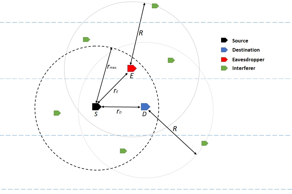
Figure 1: General V2V Scenario.

Consider a system of nodes operating in a vehicular network. We designate three nodes of interest: the information source vehicle ($S$), the information destination vehicle ($D$) and a passive eavesdropper vehicle ($E$). The vehicle $S$ transmits information to the desired vehicle $D$, while $E$ attempts to receive and decode the confidential information. Furthermore, the presence of other vehicular nodes operating within the same space and frequency band, results in co-channel interference to the received signals of $D$ and $E$. Moreover, while $D$ and $E$ are known to lie within a certain maximum radius $r_{\textrm{max}}$ from $S,$ the precise relative distances of the vehicle-to-vehicle (V2V) links are unknown during transmission, which is a realistic assumption for a network of this nature [20, 10].

The received signals at $D$ and $E$ are respectively represented as

$$y_{D} =h_{D}x+{\displaystyle{\displaystyle\sum_{k=1}^{K}h_{D_{k}}}x_{k}+}w_{D},$$ (1)

$$y_{E} =h_{E}x+{\displaystyle\sum_{k=1}^{K}}h_{E_{k}}x_{k}+w_{E},$$ (2)

where $x$ and $x_{k}$ are the respective transmitted signals by $S$ and the $k$-th interferer, with powers $P_{s}$ and $P_{k}$. The terms $w_{D}$ and $w_{E}$ are the respective additive white Gaussian noise (AWGN) at $D$ and $E$. Without loss of generality, we denote the power spectral density of the AWGN as $N_{0}$ and equal at both links. The terms $h_{i}=\sqrt{g_{i}r_{i}^{-\beta}}\quad i\in\left\{D,E\right\}$ is the channel coefficient from $S$ to the receiving vehicles $D$ and $E,$ where $r_{i}$ is the V2V link distance, $\beta$ is the path-loss exponent and $g_{i}$ is the channel gain following double Rayleigh fading [10]. As far as the intereferers are concerned, $K$ denotes the number of interference nodes, while $h_{i_{k}}=\sqrt{g_{i_{k}}r_{i_{k}}^{-\beta}}\quad i\in\left\{D,E\right\}$ is the channel coefficient between the $k$th interferer at a distance $r_{k_{i}}$ from the receiving node, and $g_{i_{k}}$ is the $k$-th interferer chananel gain.

Based on (1) and (2), the instanstaneous SINRs at $D$ and $E$ are given by

$$\gamma_{D}=\frac{P_{s}\mid h_{D}\mid^{2}}{\sum_{k=1}^{K}P_{k}\mid h_{D_{k}}\mid^{2}+N_{0}},$$ (3)

and

$$\gamma_{E}=\frac{P_{s}\mid h_{E}\mid^{2}}{\sum_{k=1}^{K}P_{k}\mid h_{E_{k}}\mid^{2}+N_{0}}.$$ (4)

III Secrecy Capacity Analysis

In this section, we derive analytical expressions for the secrecy capacity of the system. The maximum achievable secrecy capacity is defined by [21]

$$C_{s}=\max\left\{C_{D}-C_{E},0\right\},$$ (5)

where $C_{D}=\log_{2}\left(1+\gamma_{D}\right)$ and $C_{E}=\log_{2}\left(1+\gamma_{E}\right)$ are the instantaneous capacities of the main and eavesdropping links respectively. The secrecy capacity in (5) can therefore be expressed as [21]

$$C_{s}=\begin{cases}\log_{2}\left(1+\gamma_{D}\right)-\log_{2}\left(1+\gamma_{E}\right),&\gamma_{D}>\gamma_{E},\\ 0,&\gamma_{D}<\gamma_{E}.\end{cases}$$ (6)

III-A Average Secrecy Capacity

The average secrecy capacity $\overline{C_{s}}$ is given by [22]

$$\overline{C_{s}} =\mathbb{E}\left[C_{s}\left(\gamma_{D},\gamma_{E}\right)\right]$$

$$=\stackrel{{\scriptstyle[}}{{0}}]{\infty}{\int}\stackrel{{\scriptstyle[}}{{0}}]{\infty}{\int}C_{s}\left(\gamma_{D},\gamma_{E}\right)f\left(\gamma_{D},\gamma_{E}\right)\textrm{d}\gamma_{D}\textrm{d}\gamma_{E},$$ (7)

where $\mathbb{E}\left[\cdot\right]$ is the expectation operator and $f\left(\gamma_{D},\gamma_{E}\right)$ is the joint PDF of $\gamma_{D}$ and $\gamma_{E}$. It is worth noting at this point that the average in (7) is with respect to $\gamma_{D}$ and $\gamma_{E}$. However, assuming each SINR term has $L$ RVs, then we would in turn require at least $L$-fold numerical integrations to average out the RVs {$g_{D},g_{D_{1}}\ldots g_{D_{K}},g_{E},g_{E_{1}}\ldots g_{E_{K}},r_{D},$$r_{E},r_{D_{1}}\ldots$$r_{D_{k}}$ and $r_{E_{1}}\ldots r_{E_{k}}$} contained within each SINR term. Obtaining a closed-form solution would be at least arduous, if not impossible. However, the computational complexity of the task is greatly reduced by adopting the MGF approach, as mentioned earlier.

We commence by expressing the logarithmic function in (5) in an alternate form. Recalling the identity [23, Eq. (6)]

$$\textrm{ln}\left(1+x\right)=\stackrel{{\scriptstyle[}}{{0}}]{\infty}{\int}\frac{1}{s}\left(1-e^{-xs}\right)e^{-s}\textrm{d}s,$$ (8)

and by substituting $x=\gamma_{D}$ in (8), we can express the instantaneous capacity of the main link as

$$C_{D}=\frac{1}{\textrm{ln}\left(2\right)}\stackrel{{\scriptstyle[}}{{0}}]{\infty}{\int}\frac{1}{s}\left(1-e^{-s\frac{P_{s}\mid h_{D}\mid^{2}}{\sum_{k=1}^{K}P_{k}\mid h_{D_{k}}\mid^{2}+N_{0}}}\right)e^{-s}\textrm{d}s,$$ (9)

which after an interchange of variables $s=z\left(\sum_{k=1}^{K}P_{k}\mid h_{D_{k}}\mid^{2}+N_{0}\right)$ and some algebraic manipulations, we obtain an expression in the desired form with the RVs appearing only in the exponent. Thus,

$$C_{D}=\frac{1}{\textrm{ln}\left(2\right)}\stackrel{{\scriptstyle[}}{{0}}]{\infty}{\int}\frac{1}{z}e^{-zN_{0}}\times\\ \left(e^{-z\sum_{k=1}^{K}P_{k}\mid h_{D_{k}}\mid^{2}}-e^{-zP_{s}\mid h_{D}\mid^{2}}e^{-z\sum_{k=1}^{K}P_{k}\mid h_{D_{k}}\mid^{2}}\right)\textrm{d}z,$$ (10)

and after taking the expectation, we obtain the average capacity of the main link as

$$\overline{C_{D}} =\mathbb{E}\left[\textrm{ln}\left(1+\frac{P_{s}\mid h_{D}\mid^{2}}{\sum_{k=1}^{K}P_{k}\mid h_{D_{k}}\mid^{2}+N_{0}}\right)\right]$$

$$=\frac{1}{\textrm{ln}\left(2\right)}\stackrel{{\scriptstyle[}}{{0}}]{\infty}{\int}\frac{1}{z}e^{-zN_{0}}\left(\mathcal{M}_{\phi_{D}}\left(z\right)-\mathcal{M}_{\chi_{D},\phi_{D}}\left(z\right)\right)\textrm{d}z,$$ (11)

where $\mathcal{M}_{\phi_{D}}\left(z\right)=\mathbb{E}\left[e^{-z\sum_{k=1}^{K}P_{k}g_{D_{k}}r_{D_{k}}^{-\beta}}\right]$ is the MGF of the cumulative interference at $D$ and $\mathcal{M}_{\chi_{D},\phi_{D}}\left(z\right)=\mathbb{E}\left[e^{-z\left(P_{s}g_{D}r_{D}^{-\beta}+\sum_{k=1}^{K}P_{k}g_{D_{k}}r_{D_{k}}^{-\beta}\right)}\right]$ is the joint MGF of the eavesdropping link and cumulative interference at $D$. Using similar analysis, the average capacity of the eavesdropper link can be represented as

$$\overline{C_{E}}=\frac{1}{\textrm{ln}\left(2\right)}\stackrel{{\scriptstyle[}}{{0}}]{\infty}{\int}\frac{1}{z}e^{-zN_{0}}\left(\mathcal{M}_{\phi_{E}}\left(z\right)-\mathcal{M}_{\chi_{E},\phi_{E}}\left(z\right)\right)\textrm{d}z,$$ (12)

where $\mathcal{M}_{\phi_{E}}\left(z\right)$ is the MGF of the cumulative interference at $E$ and $\mathcal{M}_{\chi_{E},\phi_{E}}\left(z\right)$ is the joint MGF of the eavesdropper link and cumulative interference at $E$.

From (11), (12) and (6), the alternate form for the average secrecy capacity in (7) can be represented as

$$\overline{C_{s}}=\frac{1}{\textrm{ln}\left(2\right)}\stackrel{{\scriptstyle[}}{{0}}]{\infty}{\int}\frac{1}{z}e^{-zN_{0}}\left(\mathcal{M}_{\phi_{D}}\left(z\right)-\mathcal{M}_{\chi_{D},\phi_{D}}\left(z\right)\right)\textrm{d}z\\ -\frac{1}{\textrm{ln}\left(2\right)}\stackrel{{\scriptstyle[}}{{0}}]{\infty}{\int}\frac{1}{z}e^{-zN_{0}}\left(\mathcal{M}_{\phi_{E}}\left(z\right)-\mathcal{M}_{\chi_{E},\phi_{E}}\left(z\right)\right)\textrm{d}z.$$ (13)

From (13) we observe that the integrals are symmetrical and differ mainly in the relative locations of $S,$ $D$ and $E.$ Therefore, this signifies the importance of taking into account the node locations in the analysis. In what follows, we compute the MGFs presented in (13).

III-B Computation of Moment Generating Functions

III-B1 The MGF $\mathcal{M}_{\phi_{D}}\left(z\right)$

The MGF of the cumulative interference at $D$ is given by $\mathcal{M}_{\phi_{D}}\left(z\right)=\mathbb{E}\left[e^{-z\sum_{k=1}^{K}P_{k}g_{D_{k}}r_{D_{k}}^{-\beta}}\right]$, defined by

$$\mathcal{M}_{\phi_{D}}\left(z\right) =\mathbb{E}\left[e^{-z\sum_{k=1}^{K}P_{k}g_{D_{k}}r_{D_{k}}^{-\beta}}\right]$$

$$=\prod_{k=1}^{K}\mathbb{\mathbb{E}}\left[e^{-zP_{k}g_{D_{k}}r_{D_{k}}^{-\beta}}\right]$$

$$=\prod_{k=1}^{K}\stackrel{{\scriptstyle[}}{{g}}]{}{\int}\stackrel{{\scriptstyle[}}{{r}}]{}{\int}e^{-zP_{k}g_{D_{k}}r_{D_{k}}^{-\beta}}f_{r_{D}}(r)f_{g_{D}}(g)\textrm{d}r_{D}\textrm{d}g_{D}$$ (14)

where $f_{g_{D}}(g)$ and $f_{r_{D}}(r)$ are the probability density functions (PDFs) of the channel gain $g_{D_{k}}$and interferer distances $r_{D_{k}}$ respectively.

Let us start by defining a special case of the MGF in (14) with only the RVs, given by

$$\mathcal{M}_{\psi}\left(z\right) =\mathbb{E}\left[e^{-zg_{D_{k}}r_{D_{k}}^{-\beta}}\right]$$

$$=\stackrel{{\scriptstyle[}}{{g}}]{}{\int}\stackrel{{\scriptstyle[}}{{r}}]{}{\int}e^{-zg_{D}r_{D}^{-\beta}}f_{r_{D}}(r)f_{g_{D}}(g)\textrm{d}r_{D}\textrm{d}g_{D},$$ (15)

then from the generalized cascaded Rayleigh distribution, we can obtain the PDF of the double Rayleigh channel for $n=2$ in [24, Eq. (8)] as

$$f\left(g\right)=\textrm{G}_{0,2}^{2,0}\left(\frac{1}{4}g^{2}\Biggl{|}\negthickspace\begin{array}[]{c}-\\ \frac{1}{2},\negthickspace\frac{1}{2}\end{array}\negthickspace\right),$$ (16)

where $\textrm{G}_{u,v}^{s,t}\left(x\mid\cdots\right)$ is the Meijer’s G-function [25, Eq. (9.302)]. The node distances $r_{D},$ are assumed to be uniformly distributed within a circular region, with radius $R$ around the receiver, with a PDF given by [26]

$$f\left(r\right)=\begin{cases}\frac{2r}{R^{2}},&0<r_{D}\leq R,\\ 0,&\textrm{otherwise.}\end{cases}$$ (17)

Upon invoking [27, Eq. (2.33.10)] along with some manipulations (for $\beta>2$), the inner integral in (14) resolves to

$$\stackrel{{\scriptstyle[}}{{0}}]{R}{\int}e^{-zg_{D}r_{D}^{-\beta}}\frac{2r_{D}}{R^{2}}\textrm{d}r_{D}=\\ \frac{R^{2}e^{-zgR^{-\beta}}-\left(zg\right){}^{\frac{2}{\beta}}\Gamma\left(1-\frac{2}{\beta},zgR^{-\beta}\right)}{R^{2}},$$ (18)

where $\Gamma\left(a,b\right)=\int_{b}^{\infty}t^{a-1}e^{-t}dt$ is the upper incomplete Gamma function [27, Eq. (9.14.1)]. Thus, (15) becomes

$$\mathcal{M}_{\psi}\left(z\right)=\stackrel{{\scriptstyle[}}{{0}}]{\infty}{\int}\textrm{G}_{0,2}^{2,0}\left(\frac{1}{4}g^{2}\Biggl{|}\negthickspace\begin{array}[]{c}-\\ \frac{1}{2},\negthickspace\frac{1}{2}\end{array}\negthickspace\right)\times\qquad\qquad\\ \qquad\frac{R^{2}e^{-zgR^{-\beta}}-\left(zg\right){}^{\frac{2}{\beta}}\Gamma\left(1-\frac{2}{\beta},zgR^{-\beta}\right)}{R^{2}}\textrm{ d}g_{D},$$ (19)

which after several manipulations can be expressed as in (20) shown on top of the page, where ${}_{\phantom{}p}F_{q}\left(\alpha;\beta;z\right)$ is the generalized hypergeometric series [27, Eq. (9.14.1)].

$$\mathcal{M}_{\psi}\left(z\right)=\frac{R^{\beta}\left(2R^{\beta}\left(1-R^{-2\beta}z^{2}\right)^{\frac{1}{2}}+2z\arcsin\left(zR^{-\beta}\right)-\pi z\right)}{2\left(R^{2\beta}-z^{2}\right)\left(1-z^{2}R^{-2\beta}\right)^{\frac{1}{2}}}-\frac{\left(2z\right)^{\frac{2}{\beta}}\Gamma\left(1+\frac{1}{\beta}\right)^{2}\Gamma\left(1-\frac{2}{\beta}\right)}{R^{2}}\\ \qquad+\frac{2\pi\beta z}{R^{\beta}}\left[\frac{{}_{\,3}F_{2}\left(\frac{3}{2},\frac{3}{2},\frac{1}{2}-\frac{1}{\beta};\frac{1}{2},\frac{3}{2}-\frac{1}{\beta};z^{2}R^{-2\beta}\right)}{4\left(\beta-2\right)}-\frac{z_{\,3}F_{2}\left(2,2,1-\frac{1}{\beta};\frac{3}{2},2-\frac{1}{\beta};z^{2}R^{-2\beta}\right)}{\pi\left(\beta-1\right)R^{\beta}}\right].$$ (20)

 

Therefore, using (19) in (14), we obtain the desired MGF of interferer statistics at $D$ as

$$\mathcal{M}_{\phi_{D}}\left(z\right) =\prod_{k=1}^{K}\mathcal{M}_{\psi}\left(zP_{k}\right)$$

$$=\left\{\mathcal{M}_{\psi}\left(zP_{K}\right)\right\}^{K},$$ (21)

where the final step in (21) was obtained by assuming identical transmit powers for interferer nodes, such that $P_{1}=P_{2}=\dots=P_{k}=P_{K}.$

III-B2 The Joint MGF $\mathcal{M}_{\chi_{D},\phi_{D}}\left(z\right)$

The joint MGF $\mathcal{M}_{\chi_{D},\phi_{D}}\left(z\right)$ is given by

$$\mathcal{M}_{\chi_{D},\phi_{D}}\left(z\right) =\mathbb{E}\left[e^{-zP_{s}g_{D}r_{D}^{-\beta}+\sum_{k=1}^{K}P_{k}g_{D_{k}}r_{D_{k}}^{-\beta}}\right]$$

$$=\mathbb{E}\left[e^{-zP_{s}g_{D}r_{D}^{-\beta}}e^{-z\sum_{k=1}^{K}P_{k}g_{D_{k}}r_{D_{k}}^{-\beta}}\right]$$

$$=\mathcal{M}_{\chi_{D}}\left(z\right)\mathcal{M}_{\phi_{D}}\left(z\right),$$ (22)

where $\mathcal{M}_{\phi_{D}}\left(z\right)$ is given by the expression (21) and $\mathcal{M}_{\chi_{D}}\left(z\right)$ is the MGF of statistics at $D.$ It is worth noting that the system considered assumes the location of $D$ is known by $S.$ Consequently, $r_{D}$ is not random and the MGF is conditioned only on the statistics of the channel. Thus, the expected value for the first MGF in (22) is given by

$$\mathcal{M}_{\chi_{D}}\left(z\right) =\mathbb{E}\left[\exp\left(-zP_{s}g_{D}r_{D}^{-\beta}\right)\right]$$

$$=\stackrel{{\scriptstyle[}}{{0}}]{\infty}{\int}e^{-zP_{s}g_{D}r_{D}^{-\beta}}\textrm{G}_{0,2}^{2,0}\left(\frac{1}{4}g^{2}\Biggl{|}\negthickspace\begin{array}[]{c}-\\ \frac{1}{2},\negthickspace\frac{1}{2}\end{array}\negthickspace\right)\textrm{ d}g_{D}.$$ (25)

To proceed, we express (25) in a more tractable form, by re-writing the Meijer G-function in an alternate form. Thus, upon invoking [27, Eq. (9.304.3)], we get

$$\textrm{G}_{0,2}^{2,0}\left(\frac{1}{4}g^{2}\Biggl{|}\negthickspace\begin{array}[]{c}-\\ \frac{1}{2},\negthickspace\frac{1}{2}\end{array}\negthickspace\right)=gK_{0}\left(g\right),$$ (26)

where $K_{0}\left(v\right)$ is the modified Bessel function of the second kind and $0$th order [27, Eq. (8.407)]. Using (26) and [27, Eq. (6.621.3)] along with some basic algebraic manipulations, we can straightforwardly obtain the desired result as

$$\mathcal{M}_{\chi_{D}}\left(z\right)=\frac{4}{3(1+zP_{s}r_{D}^{-\beta})^{2}}{}_{\phantom{}2}F_{1}\left(2,\frac{1}{2},\frac{5}{2},\frac{zP_{s}r_{D}^{-\beta}-1}{zP_{s}r_{D}^{-\beta}+1}\right),$$ (27)

where ${}_{\phantom{}2}F_{1}\left(\alpha;\beta;\gamma;z\right)$ is the Gauss hypergeometric function [27, Eq. (9.111)]. Hence, we obtain $\mathcal{M}_{\chi_{D},\phi_{D}}\left(z\right)$ by substituting (20), (22) and (27) in (22).

III-B3 The MGF $\mathcal{M}_{\phi_{E}}\left(z\right)$

The MGF of the cumulative interference at $E$ is given by $\mathcal{M}_{\phi_{E}}\left(z\right)=\mathbb{E}\left[e^{-z\sum_{k=1}^{K}P_{k}g_{E_{k}}r_{E_{k}}^{-\beta}}\right]$. From the definition of the MGF, it can be observed that the computation of $\mathcal{M}_{\phi_{E}}\left(z\right)$ follows similar analysis to the interference at $D$. Due to brevity, the analysis will not be repeated here. Thus, using (20), the desired MGF is given by

$$\mathcal{M}_{\phi_{E}}\left(z\right)=\left\{\mathcal{M}_{\psi}\left(zP_{K}\right)\right\}^{K}.$$ (28)

III-B4 The Joint MGF $\mathcal{M}_{\chi_{E},\phi_{E}}\left(z\right)$

The joint MGF $\mathcal{M}_{\chi_{E},\phi_{E}}\left(z\right)$ can be obtained through similar analysis presented in Sec. III-B2, Therefore, from (22), $\mathcal{M}_{\chi_{E},\phi_{E}}\left(z\right)=\mathcal{M}_{\chi_{E}}\left(z\right)\mathcal{M}_{\phi_{E}}\left(z\right)$, where $\mathcal{M}_{\phi_{E}}\left(z\right)$ is given by (28). For the purpose of the system under consideration, the exact location of $E$ is unknown, but lies at a maximum distance $r_{\max}$ from $S$. Using the PDFs in (16) and (17), we obtain

$$\mathcal{M}_{\chi_{E}}\left(z\right)=\mathbb{E}\left[\exp\left(-zP_{s}g_{E}r_{E}^{-\beta}\right)\right]\\ =\stackrel{{\scriptstyle[}}{{0}}]{\infty}{\int}\stackrel{{\scriptstyle[}}{{0}}]{r_{\max}}{\int}e^{-zP_{s}g_{E}r_{E}^{-\beta}}\frac{2r_{E}}{r_{\textrm{max}}^{2}}\textrm{G}_{0,2}^{2,0}\left(\frac{1}{4}g^{2}\Biggl{|}\negthickspace\begin{array}[]{c}-\\ \frac{1}{2},\negthickspace\frac{1}{2}\end{array}\right)\textrm{d}r_{E}\textrm{d}g_{E}.$$ (29)

Comparing (29) and (14), shows that both expressions are similar with maximum distance $R=r_{\textrm{max}}$ and source power $P_{s}$. Thus, using (20), $\mathcal{M}_{\chi_{E}}\left(z\right)=\mathcal{M}_{\psi}\left(zP_{s}|r_{\max}\right)$ and we obtain from (20) and (28) the expression

$$\mathcal{M}_{\chi_{E},\phi_{E}}\left(z\right) =\mathcal{M}_{\chi_{E}}\left(z\right)\mathcal{M}_{\phi_{E}}\left(z\right)$$

$$=\mathcal{M}_{\psi}\left(zP_{s}|r_{\max}\right)\left\{\mathcal{M}_{\psi}\left(zP_{K}\right)\right\}^{K}.$$ (30)

To recap, the average secrecy capacity is obtained from (13) by substituting the relevant MGFs from (20), (22), (27), (28) and (30).

IV Numerical Results and Discussions

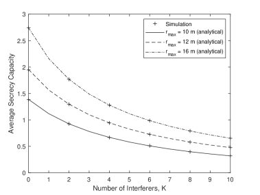
Figure 2: Average Secrecy Capacity versus Number of Interferers $K$, with varied maximum eavesdropper radius $r_{\max}$.

In this section, we present and discuss some results from the mathematical expressions derived in the paper. We then investigate the effect of key parameters on the secrecy capacity of the system. The results are then verified using Monte Carlo simulations with at least $10^{6}$ iterations. Unless otherwise stated, we have assumed source power $P_{s}=10$W, interferer transmit power $P_{K}=10$W, $S$-to-$D$ distance $r_{D}=4$m, maximum eavesdropper distance $r_{\max}=10$m, maximum interferer distance $R=20$m and pathloss exponent $\beta=2.7$.

In Fig. 2, we present a plot of the average secrecy capacity against the number of interfering sources in the network. It can be observed from the results that the number of active interfering nodes have a negative impact on the secrecy capacity, with the highest secrecy capacity available when there is no interfering node ($K=0)$ and rapidly reduces with interference. Moreover, this impact can be effective at various eavesdropper distances from the node, as seen when $r_{\max}$ is increased. It should be noted that the parameter $r_{\max}$ is a proxy for the uncertainty of $E$’s location. In a practical scenario, a vehicle is more likely to know the location of the node $D$ in which it establishes communication as against a passive eavesdropper whose presence may not be known. Therefore, we assume both $D$ and $E$ are always within the radius $r_{\max}$, while the interferer nodes are restricted by a larger outer radius of $R.$ Therefore the increased secrecy observed when $r_{\max}$ increases indicates that when $E$ is more likely to be closer to $S$-to-$D$ V2V link, then the secrecy is compromised, and vice versa.

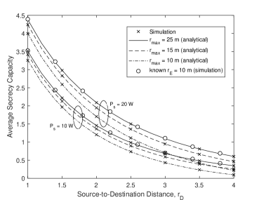
Figure 3: Average Secrecy Capacity versus source to destination ($S$-to-$D$ link) for varied source transmit power $P_{s}$ and known eavesdropper distance $r_{E}$.

Fig. 3, shows a plot of the average secrecy capacity against the $S$-to-$D$ distance $r_{D}$, with different values of $P_{s}$ and $r_{\max}.$ We assume $R=40$m and $5$ interfering nodes. First, we observe that the average secrecy capacity decreases as $D$ moves away from $S$, which is expected because the SINR at $D$ is also decreasing. Next, we see the effect of increasing the maximum range of $E.$ At the different $P_{s}$ values, we observe that increasing $r_{\max}$ improves the secrecy capacity because this means the likely radius of finding $E$ is extended. However, as $r_{\max}$ is reduced, the secrecy capacity rapidly decreases and reaches zero approximately when $r_{D}=\nicefrac{{1}}{{2}}r_{\max}.$ This shows the significance of the relative locations of $S,$ $D$ and $E.$ To further demonstrate this, we assume a known location for $E$ and use this distance $r_{E}$ to illustrate the significance of our result with respect to interferer impact on secrecy. We assume $r_{E}=10$m and plot the exact secrecy capacity for the V2V network, through simulations. From Fig. 3, it can be observed that the secrecy capacity for known $r_{E}$ is much superior to the case when $E$’s location is uncertain. In fact, from our analysis, it can be seen that the secrecy capacity at $r_{E}=10$m is equivalent to the secrecy capacity when $r_{\max}=25$m within the region studiesd. This therefore signifies the importance of taking into account the uncertainty of the location of $E$, especially for the security analysis of passive eavesdroppers, when the eavesdropper is unlikely to give away its position by transmissions.

In Fig. 4, we present the average secrecy capacity with respect to $P_{s}$ for different number of interfering nodes $K$ and maximum interferer range $R$. As expected, the secrecy capacity increases monotonically with increased $P_{s}$. Furthermore, within the region investigated, the average secrecity capacity is highest without any interfering nodes and degrades with more active interfering nodes, as already demonstrated in the previous figure. Additionally, it can be observed that for the same number of interferers, increasing $R,$ improves the secrecy capacity of the system. Given that both $S$ and $E$ are affected by the interference in the network, then an increased radius of interferers, reduces the density of interfering nodes, which in turn improves the secrecy capacity.

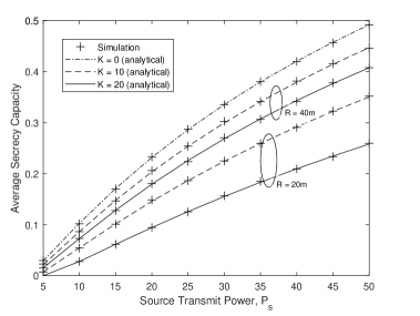
Figure 4: Average Secrecy Capacity versus Source Transmit Power $P_{s}$ for varied interferer numbers $K$ and maximum interferer distances $R.$

V Conclusions

In this paper, we examined the impact of interference on the secrecy capacity as a key metric for physical layer security of a wireless vehicular communication network. Due to the nature of the network and statistics of the SINR, we expressed the capacity in terms of the MGF of the RVs representing the joint fading and random distances of interfering nodes, and eavesdropper node. This reduced the complexity of the solution. We found closed-form expressions for the various MGFs and used these expressions to calculate the average secrecy capacity of the system. The close agreement between the analytical and simulated results clearly indicated the validity of the derived expressions. The results demonstrated the effect of some key system parameters such as the distances of the V2V node distances and eavesdropper, as well as the number and distances of interference nodes. The results showed the importance of the analysis with respect to considering uncertainty of the eavesdropper location, by showing a significant reduction in secrecy capacity when location of eavesdropper is not known. The results also showed the effect of interfering nodes on the security of the system, there by further highlighting the importance of our analysis.

References

- [1] Y. Y. Zu and K. Xiao, “Outage performance of secure cooperative systems over correlated rayleigh fading channels,” in 2016 25th Wireless and Optical Commun. Conf. (WOCC), May 2016, pp. 1–5.
- [2] G. C. Alexandropoulos and K. P. Peppas, “Secrecy outage analysis over correlated composite Nakagami- /Gamma fading channels,” IEEE Commun. Lett., vol. 22, no. 1, pp. 77–80, Jan. 2018.
- [3] M. Z. I. Sarkar, T. Ratnarajah, and M. Sellathurai, “Secrecy capacity of Nakagami- fading wireless channels in the presence of multiple eavesdroppers,” in Asilomar Conf. Sig. Sys. Comput., Nov. 2009, pp. 829–833.
- [4] M. Srinivasan and S. Kalyani, “Secrecy capacity of shadowed fading channels,” IEEE Commun. Lett., vol. 22, no. 8, pp. 1728–1731, Aug. 2018.
- [5] N. Bhargav and S. L. Cotton, “Secrecy capacity analysis for - /- and - / - fading scenarios,” in 2016 IEEE 27th Annual Int. Symp. Personal, Indoor, and Mobile Radio Commun. (PIMRC), Sep. 2016, pp. 1–6.
- [6] O. S. Badarneh, P. C. Sofotasios, S. Muhaidat, S. L. Cotton, K. Rabie, and N. Al-Dhahir, “On the Secrecy Capacity of Fisher-Snedecor F Fading Channels,” in 2018 14th Int. Conf. Wireless Mobile Comput., Netw. Commun. (WiMob), Oct. 2018, pp. 102–107.
- [7] A. Salem, K. M. Rabie, K. A. Hamdi, E. Alsusa, and A. M. Tonello, “Physical layer security of cooperative relaying power-line communication systems,” in 2016 Int. Symp. Power Line Commun, and its Applications (ISPLC), Mar. 2016, pp. 185–189.
- [8] A. Salem, K. A. Hamdi, and E. Alsusa, “Physical Layer Security Over Correlated Log-Normal Cooperative Power Line Communication Channels,” IEEE Access, vol. 5, pp. 13 909–13 921, 2017.
- [9] A. Salem, K. A. Hamdi, and K. M. Rabie, “Physical Layer Security With RF Energy Harvesting in AF Multi-Antenna Relaying Networks,” IEEE Trans. Commun., vol. 64, no. 7, pp. 3025–3038, Jul. 2016.
- [10] Y. Ai, M. Cheffena, A. Mathur, and H. Lei, “On Physical Layer Security of Double Rayleigh Fading Channels for Vehicular Communications,” IEEE Wireless Commun. Lett., vol. 7, no. 6, pp. 1038–1041, Dec. 2018.
- [11] I. Dey, R. Nagraj, G. G. Messier, and S. Magierowski, “Performance analysis of relay-assisted mobile-to-mobile communication in double or cascaded Rayleigh fading,” in 2011 IEEE Pacific Rim Conf. Commun. Comput. Sign. Process., Aug. 2011, pp. 631–636.
- [12] A. S. Akki and F. Haber, “A statistical model of mobile-to-mobile land communication channel,” IEEE Trans. Veh. Tech., vol. 35, no. 1, pp. 2–7, Feb. 1986.
- [13] V. Erceg, S. J. Fortune, J. Ling, A. J. Rustako, and R. A. Valenzuela, “Comparisons of a computer-based propagation prediction tool with experimental data collected in urban microcellular environments,” IEEE J. Sel. Areas Commun., vol. 15, no. 4, pp. 677–684, May 1997.
- [14] L. Farhan, O. Kaiwartya, L. Alzubaidi, W. Gheth, E. Dimla, and R. Kharel, “Toward Interference Aware IoT Framework: Energy and Geo-Location-Based-Modeling,” IEEE Access, vol. 7, pp. 56 617–56 630, 2019.
- [15] Z. Shu, Y. Yang, Y. Qian, and R. Q. Hu, “Impact of interference on secrecy capacity in a cognitive radio network,” in Proc. IEEE Global Commun. (GLOBECOM), Dec. 2011, pp. 1–6.
- [16] D. S. Karas, A. A. Boulogeorgos, G. K. Karagiannidis, and A. Nallanathan, “Physical layer security in the presence of interference,” IEEE Wireless Commun. Lett., vol. 6, no. 6, pp. 802–805, Dec. 2017.
- [17] R. Kasana, S. Kumar, O. Kaiwartya, R. Kharel, J. Lloret, N. Aslam, and T. Wang, “Fuzzy-based channel selection for location oriented services in multichannel VCPS environments,” IEEE Internet Things J., vol. 5, no. 6, pp. 4642–4651, Dec 2018.
- [18] O. Kaiwartya, Y. Cao, J. Lloret, S. Kumar, N. Aslam, R. Kharel, A. H. Abdullah, and R. R. Shah, “Geometry-Based Localization for GPS Outage in Vehicular Cyber Physical Systems,” IEEE Trans. Veh. Tech., vol. 67, no. 5, pp. 3800–3812, May 2018.
- [19] S. Kumar, U. Dohare, K. Kumar, D. Prasad, K. N. Qureshi, and R. Kharel, “Cybersecurity measures for geocasting in vehicular cyber physical system environments,” IEEE Internet Things J., pp. 1–1, 2019.
- [20] D. S. Karas, A. A. Boulogeorgos, and G. K. Karagiannidis, “Physical layer security with uncertainty on the location of the eavesdropper,” IEEE Wireless Commun. Lett., vol. 5, no. 5, pp. 540–543, Oct. 2016.
- [21] M. Bloch, J. Barros, M. R. D. Rodrigues, and S. W. McLaughlin, “Wireless information-theoretic security,” IEEE Trans. Inf. Theory, vol. 54, no. 6, pp. 2515–2534, Jun. 2008.
- [22] O. S. Badarneh, P. C. Sofotasios, S. Muhaidat, S. L. Cotton, K. Rabie, , and N. Al-Dhahir, “On the secrecy capacity of Fisher-Snedecor fading channels,” in Proc. IEEE Global Commun. (GLOBECOM), May 2018.
- [23] K. A. Hamdi, “Capacity of MRC on correlated Rician fading channels,” IEEE Trans. Commun., vol. 56, no. 5, pp. 708–711, May 2008.
- [24] J. Salo, H. M. El-Sallabi, and P. Vainikainen, “The distribution of the product of independent Rayleigh random variables,” IEEE Trans. Antennas Propag., vol. 54, no. 2, pp. 639–643, Feb. 2006.
- [25] A. P. Prudnikov, Y. A. Brychkov, and O. I. Marichev, Integrals, and Series: More Special Functions, Gordon and Breach Sci. Publ., New York, 1990, vol. 3.
- [26] Y. Shobowale and K. Hamdi, “A unified model for interference analysis in unlicensed frequency bands,” IEEE Trans. Wireless Commun., vol. 8, no. 8, pp. 4004–4013, Aug. 2009.
- [27] I. S. Gradshteyn and I. M. Ryzhik, Table of Integrals, Series, and Products, 7th ed. Academic Press, Califonia, 2007.