Implicit Regularization and Convergence for
Weight Normalization

Abstract

Normalization methods such as batch (Ioffe and Szegedy, 2015), weight (Salimans and Kingma, 2016), instance (Ulyanov et al., 2016), and layer normalization (Ba et al., 2016) have been widely used in modern machine learning. Here, we study the weight normalization (WN) method (Salimans and Kingma, 2016) and a variant called reparametrized projected gradient descent (rPGD) for overparametrized least squares regression. WN and rPGD reparametrize the weights with a scale $g$ and a unit vector $w$ and thus the objective function becomes non-convex. We show that this non-convex formulation has beneficial regularization effects compared to gradient descent on the original objective. These methods adaptively regularize the weights and converge close to the minimum $\ell_{2}$ norm solution, even for initializations far from zero. For certain stepsizes of $g$ and $w$, we show that they can converge close to the minimum norm solution. This is different from the behavior of gradient descent, which converges to the minimum norm solution only when started at a point in the range space of the feature matrix, and is thus more sensitive to initialization.

1 Introduction

Modern machine learning models often have more parameters than data points, allowing a fine-grained adaptation to the data, but also suffering from the risk of over-fitting. To alleviate this, various explicit and implicit regularization methods are used. For instance, weight decay can control the model complexity by shrinking the norm of the weights, and dropout can reduce the model capacity by sub-sampling features during training (Gal and Ghahramani, 2016; Mianjy et al., 2018; Arora et al., 2020). Recent state-of-the-art techniques such as batch, weight, and layer normalization (Ioffe and Szegedy, 2015; Salimans and Kingma, 2016; Ba et al., 2016), empirically have a regularization effect, e.g., as described in Ioffe and Szegedy (2015), "batch normalisation acts as a regularizer, in some cases eliminating the need for dropout".

While normalization methods are practically popular and successful, their theoretical understanding has only started to emerge recently. For instance, normalization methods make learning more robust to hyperparameters such as the learning rate (Wu et al., 2018; Arora et al., 2019). Moreover, it has been argued that normalization methods can make the model robust to the shift and scaling of the inputs, preventing “internal covariate shift" (Ioffe and Szegedy, 2015) as well as smooth or modify (Santurkar et al., 2018; Lian and Liu, 2019) the optimization landscape.

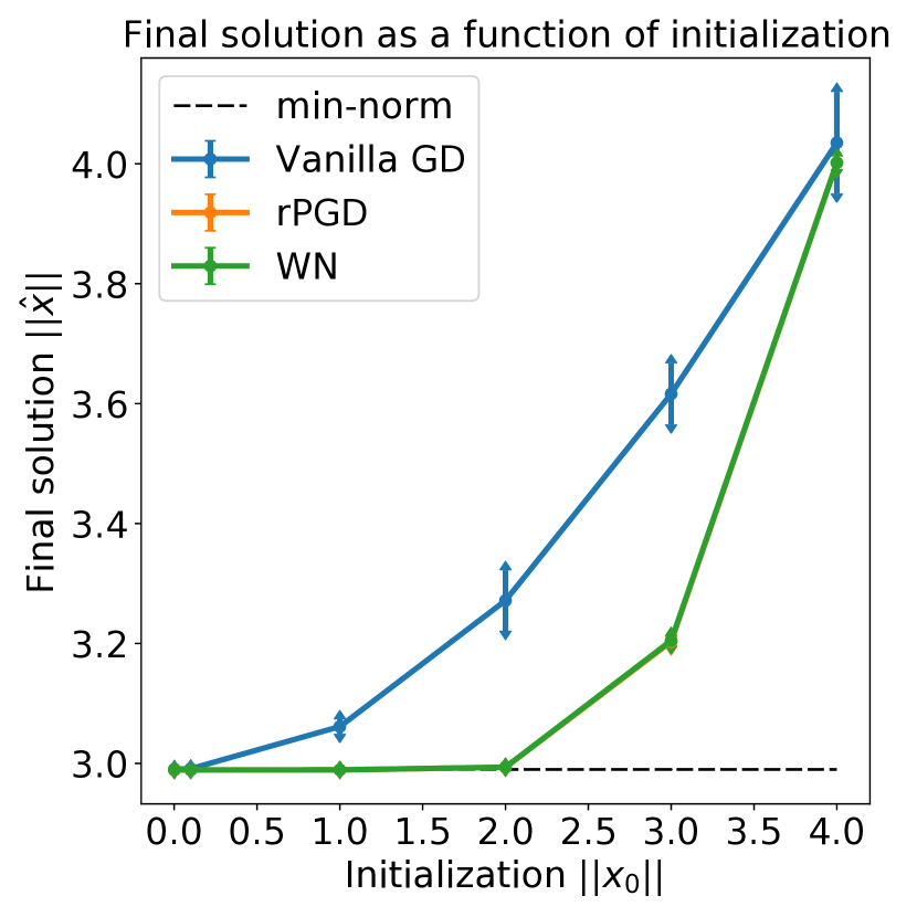
Figure 1: Comparison of the outputs $||\widehat{x}||=\|\widehat{g}\widehat{w}\|$ provided by GD, WN and rPGD on an overparametrized linear regression problem (see Section 1.1). All algorithms (with stepsizes $0.005$) start from the same initialization and stop when the loss reaches $10^{-5}$. Note that the orange (rPGD) and green (WN) curves overlap (see Lemma 2.2 for explanation and Section F for experimental details). GD converges to the minimum $\ell_{2}$-norm solution only when $\|x_{0}\|=0$, while WN and rPGD converge close to the minimum norm solution for a wider range of initializations with smaller standard deviation.

Yet, a precise characterization of the regularization effect of normalization methods in overparametrized models is not available. For overparametrized models, there are typically infinitely many global minima, as shown e.g., in matrix completion (Ge et al., 2016) and neural networks (Ge et al., 2017). Thus, we can analyze how different algorithms converge to different global minima as a way of quantifying implicit bias. It is critical for the algorithm to converge to a solution with good generalization properties, e.g., Zhang et al. (2016); Neyshabur et al. (2019), etc. For the key model of over-parameterized linear least squares, it is well-known that gradient descent (GD) converges to the minimum Euclidean norm solution when started from zero, (see e.g. Hastie et al., 2019). It has been argued that this may have favorable generalization properties in learning theory (norms can control the Radamechar complexity), as well as more recent analyses (Bartlett et al., 2019; Hastie et al., 2019; Belkin et al., 2019; Liang and Rakhlin, 2018).

However, for non-convex optimization, starting from the origin might be problematic – this is true in particular in neural networks with ReLU activation function which is often used (LeCun et al., 2015). In neural networks, we often instead apply random initialization (Glorot and Bengio, 2010; He et al., 2015) which can for instance help escape saddle points (Lee et al., 2016). Thus, it is important to study algorithms with initializations not close to zero.

With this in mind, we study how a particular normalization method, weight normalization (WN) (Salimans and Kingma, 2016), affects the choice of global minimum in overparametrized least squares regression. WN writes the model parameters $x$ as $x=gw/\|w\|_{2}$, and optimizes over the "length" $g\in\mathbb{R}$ and the unnormalized direction $\smash{w\in\mathbb{R}^{d}}$ separately. Inspired by weight normalization, we also study a related method where we parametrize the weight as $x=gw$, with $g\in\mathbb{R}$ and a normalized direction $w$ with $\|w\|_{2}=1$, (see e.g. Douglas et al., 2000). Different from WN, this method performs projected GD on the unit norm vector $v$, while WN does GD on $w$ such that $w/\|w\|$ is the unit vector. We call this variant the reparametrized projected gradient descent (rPGD) algorithm. We show that the two algorithms (rPGD and WN) have the same limit when the stepsize tends to zero. Arguing in both discrete and continuous time, we show that both find global minima robust to initialization.

Our Contributions. We consider the overparametrized least squares (LS) optimization problem, which is convex but has infinitely many global minima. As a simplified companion of WN in LS, we introduce the rPGD algorithm (Alg. 2), which is projected gradient descent on a nonconvex reparametrization of LS. We show that WN and rPGD have the same limiting flow—the WN flow—in continuous time (Lemma 2.2). We characterize the stationary points of the loss, showing that the nonconvex reparametrization introduces some additional stationary points that are in general not global minima. However, we also show that the loss still decreases at a geometric rate, if we can control the scale parameter $g$.

How to control the scale parameter? Perhaps surprisingly, we show the delicate property that the scale and the orthogonal complement of the weight vector are linked through an invariant (Lemma 2.5). This allows us to show that the WN flow converges at a geometric rate in spite of the non-convexity of the reparameterized objective. We precisely characterize the solution, and when it is close to the min norm solution.

In discrete-time, when the stepsize is not infinitely small, we first consider a simple setting where the feature matrix is orthogonal and characterize the behavior of rPGD (Theorem 3.2). We show that by appropriately lowering the learning rate for the scale $g$, rPGD converges to the minimum $\ell_{2}$ norm solution. We give sharp iteration complexities and upper bounds for the stepsize required for $g$. We extend the result to general data matrices $A$ (Theorem 3.3), where the results become more challenging to prove and a bit harder to parse. This sheds light the empirical observation that only optimizing the direction $w$ training the last layer of neural nets improves generalization (Goyal et al., 2017; Xu et al., 2019).

1.1 Setup

We use $\|\cdot\|$ for the $\ell_{2}$ norm, and consider the standard overparametrized linear regression problem:

$$\min_{x\in\mathbb{R}^{d}}\frac{1}{2}\|Ax-y\|^{2},$$ (1)

where $A\in\mathbb{R}^{m\times d}$ ($m<d$) is the feature matrix and $y\in\mathbb{R}^{m}$ is the target vector. Without loss of generality, we assume that the feature matrix $A$ has full rank $m$. This objective has infinitely many global minimizers, and among them let the minimum $\ell_{2}$-norm solution be $x^{*}$. Observe that $x^{*}$ is characterized by the two properties: (1) $Ax^{*}=y$; (2) $x^{*}$ is in the row space of the matrix $A$. We can describe condition (2) via Definition 1.1.

Definition 1.1.

For any $z\in\mathbb{R}^{d}$, we can write $z=z^{\parallel}+z^{\perp}$ where $Az^{\parallel}=Az\text{ and }Az^{\perp}=0.$

Then we can equivalently write condition (2) as $x^{*\parallel}=x^{*}.$ We focus on weight normalization and a related reparametrized projected gradient descent method. Notably, both transform the original convex LS problem to a non-convex problem, which increases the difficulty of theoretical analysis.

Weight normalization (WN)

WN reparametrizes the variable $x$ as $g\cdot w/\|w\|$, where $g\in\mathbb{R}$ and $w\in\mathbb{R}^{d}$, which leads to the following minimization problem:

$$\min_{g\in\mathbb{R},w\in\mathbb{R}^{d}}h(w,g)=\frac{1}{2}\left\|gAw/\|w\|-y\right\|^{2}.$$ (2)

We can write the min norm solution as $x^{*}=g^{*}w^{*}/\|w^{*}\|$, where $w^{*}$ is unique up to scale. However, we can always choose $w^{*}$ so that $g^{*}>0$, unless $x^{*}=0$, which implies that $y=0$. We exclude this degenerate case throughout the paper. The discrete time WN algorithm is shown in Algorithm 1.

  Input: Unit norm $w_{0}$ and scalar $g_{0}$,iterations $T$, step-sizes $\{\gamma_{t}\}_{t=0}^{T-1}$ and $\{\eta_{t}\}_{t=0}^{T-1}$

  for $t=0,1,2,\cdots,T-1$ do

    $w_{t+1}=w_{t}-\eta_{t}\nabla_{w}h(w_{t},g_{t})$

    $g_{t+1}=g_{t}-\gamma_{t}\nabla_{g}h(w_{t},g_{t})$

    

  end for

Algorithm 1 WN for (2)

  Input: Unit norm $w_{0}$ and $g_{0}$, number of iterations $T$, step-sizes $\{\gamma_{t}\}_{t=0}^{T-1}$ and $\{\eta_{t}\}_{t=0}^{T-1}$

  for $t=0,1,2,\cdots,T-1$ do

    $v_{t}=w_{t}-\eta_{t}\nabla_{w}f(w_{t},g_{t})$ (gradient step)

    $w_{t+1}=\frac{v_{t}}{\|v_{t}\|}$    (projection)

    $g_{t+1}=g_{t}-\gamma_{t}\nabla_{g}f(w_{t},g_{t})$ (gradient step)

  end for

Algorithm 2 rPGD for (3)

Reparametrized Projected Gradient Descent (rPGD)

Inspired by WN algorithm, we investigate an algorithm that directly updates the direction of $w$. See Douglas et al. (2000) for an example of such algorithms. Since the direction is a unit vector, we can perform projected gradient descent on it. To be more concrete, we reparametrize the variable $x$ as $gw$, where $g$ denotes the scale and $w\in\mathbb{R}^{d}$ with $\|w\|=1$ denotes the direction, and transform (2) into the following problem:

$$\min_{g\in\mathbb{R},w\in\mathbb{R}^{d}}f(w,g):=\frac{1}{2}\|Agw-y\|^{2},\quad\textnormal{s.t.}\quad\|w\|=1.$$ (3)

The minimum norm solution can be uniquely written as $x^{*}=g^{*}w^{*}$, where $g^{*}>0$ and $\|w^{*}\|=1$. To solve (3), we update $g$ with standard gradient descent, and update $w$ via projected gradient descent (PGD) (see Algorithm 2). We call this algorithm reparameterized PGD (rPGD).

One may observe that both algorithms can heuristically be viewed as a variation of adaptive $\ell_{2}$ regularization, where the magnitude of the regularization depends on the current iteration. We refer the readers to Appendix A for a detailed discussion.

2 Continuous Time Analysis

In this section, we study the properties of a continuous limit of WN and rPGD, to give insight into the implicit regularization of normalization methods. We use constant stepsizes for both the update of the scale $g$ and weight $w$, and take them to zero in a way that their ratio remains a constant.

Condition 2.1 (Stepsizes).

For both Algorithms 1 and 2, use constant stepsizes $\eta_{t}=\eta$ and $\gamma_{t}=c\eta$ for $g$ and $w$ respectively, with $c\geq 0$ a fixed constant ratio. We take the continuous limit $\eta\to 0$.

Setting $c=0$ amounts to fixing $g$ and only updating $w$. We first prove that the continuous limit of the dynamics of $(g_{t},w_{t}/\|w_{t}\|)$ for WN evolves the same as the continuous limit of the dynamics of $(g_{t},w_{t})$ for rPGD, assuming we start with $\|w_{0}\|=1$ for WN. The proof can be found in Appendix B.

Lemma 2.2 (Limiting flow for WN and rPGD).

Assume Condition 2.1 and that $\|w_{0}\|=1$ for WN. Then WN (Algorithm 1) with $(g_{t},w_{t}/\|w_{t}\|)$ and rPGD (Algorithm 2) with $(g_{t},w_{t})$ have the same limiting dynamics, which we call WN flow. This is given by the pair of ordinary differential equations

$$\frac{dg_{t}}{dt}=-c\nabla_{g}f(w_{t},g_{t}) \quad\frac{dw_{t}}{dt}=-g_{t}\mathcal{P}_{t}\left(\nabla_{w}f(w_{t},g_{t})\right).$$ (4)

Here $f$ is from (3). With $r=y-Agw$ to denote the residual, $\nabla_{w}f=A^{\top}r$, $\nabla_{g}f=w^{\top}A^{\top}r$, and $\mathcal{P}_{t}=I-w_{t}w_{t}^{\top}/\|w_{t}\|^{2}$ the projection matrix onto the space orthogonal to $w_{t}$.

While the flow is valuable, the nonconvex reparametrization introduces some new stationary points. We characterize them, and later use this to understand the convergence.

Lemma 2.3 (Stationary points).

Suppose the smallest eigenvalue of $AA^{\top}$, is positive, $\lambda_{\min}:=\lambda_{\min}(AA^{\top})>0$. The stationary points of the reparameterized loss from (2) either (a) have loss equal to zero, or (b) belong to the set $\mathcal{S}:=\{(g,w):g=0,y^{\top}Aw=0\}.$ If the loss (2) at $g,w$ is strictly less than the loss at $(g=0,w)$, i.e. $\|y\|^{2}>\|Agw-y\|^{2}$, we are always in case (a).

It is a folklore result that under gradient flow, the loss is non-increasing even in the nonconvex case (see e.g. Rockafellar and Wets, 2009). For the WN gradient flow, we can make this folklore rigorous and, provided the scale parameter $g_{t}$ is lower bounded, show that the loss decreases at a geometric rate.

Lemma 2.4 (Rate of $\|r_{t}\|$).

Under the setting of Lemma 2.2, we have the bounds:

$$-\max\{g_{t}^{2},c\}\|A^{\top}r_{t}\|^{2}\leq d[1/2\|r_{t}\|^{2}]/dt\leq-\min\{g_{t}^{2},c\}\|A^{\top}r_{t}\|^{2}\leq 0.$$ (5)

This shows that $\|r_{t}\|$ is non-increasing. If for some $C>0$, $g_{t}>C$ for all $t$, then the loss decreases geometrically at rate $\min(C^{2},c)$.

How can we control the scale parameter? Perhaps surprisingly, we show that the scale parameter and the orthogonal complement of the weight vector are linked through an invariant.

Lemma 2.5 (Invariant).

Assume $c>0$ in Condition 2.1. Under the setting from Lemma 2.2, let $\smash{w_{t}=w_{t}^{\perp}+w_{t}^{\parallel}}$ as defined in Definition 1.1. We have at time $t>0$,

$$w_{t}^{\perp}=\exp\left({\frac{g_{0}^{2}-g_{t}^{2}}{2c}}\right)w_{0}^{\perp}\quad\text{and so}\quad\|w_{t}^{\perp}\|^{2}\cdot\exp(g_{t}^{2}/2c)=\|w_{0}^{\perp}\|^{2}\cdot\exp(g_{0}^{2}/2c).$$ (6)

Lemma 2.5 shows that the orthogonal complement $w_{t}^{\perp}$ can change during the WN flow dynamics. This is the key property of WN that can yield additional regularization. Lemma 2.5 also implies that $\|w_{t}^{\perp}\|^{2}\cdot\exp(g_{t}^{2}/2c)$ is invariant along the path. If we initialize with small $|g_{0}|$ and $|g_{t}|$ is greater than $|g_{0}|$ (we will describe the dynamics of $g_{t}$ in the next part), then $\|w_{t}^{\perp}\|^{2}$ will decrease, and we get close to the minimum norm solution. This is in contrast to gradient descent and flow, where $\|w^{\perp}\|^{2}$ is preserved (see e.g.,  (Hastie et al., 2019)).

The invariant (6) in the optimization path holds for certain more general settings. Specifically, it holds for linearly parametrized loss functions that only depend on a small dimensional linear subspace of the parameter space (e.g., overparametrized logistic regression). See Appendix D. Equipped with the above lemmas, we can discuss the solution and implicit regularization effect of the WN flow.

Theorem 2.6 (WN flow Solution).

Assume Condition 2.1 and $\lambda_{\min}>0$. Suppose we initialize the WN flow at $g_{0},w_{0}$, such that $\|w_{0}\|=1$. We have that either (a) the loss converges to zero, or (b) the iterates $(g_{t},w_{t})$ converge to a stationary point in $\mathcal{S}$ as defined in Lemma 2.3. In case (a), we characterize the solutions based on $g_{t}$:

• If $c>0$, and the loss converges to zero, the solution can be expressed as

  $$\lim_{t\to\infty}g_{t}w_{t}=x^{*}+g^{*}w_{0}^{\perp}\exp\left(\frac{g_{0}^{2}-g^{*2}}{2c}\right).$$ (7)

• If $c=0$ and $A$ is orthogonal, i.e., $AA^{\top}=I$, then $w_{t}\to w^{*}$. If $A$ is not orthogonal, then the flow still converges to a point $\tilde{w}_{0}$ in the row space of $A$ (i.e, $\tilde{w}_{0}^{\perp}=0$). When restarting the WN flow with $c>0$ from $g_{0},\tilde{w}_{0}$, then $(g_{0},\tilde{w}_{0})\to(g^{*},w^{*})$.

We defer the proofs of Lemmas 2.4, 2.5 and Theorem 2.6 to Appendix C. Part I of Theorem 2.6 shows that, if we initialize with $g_{0}^{2}\leq g^{*2}$ and we are not stuck at $\mathcal{S}$, the WN flow will converge to a solution that is close to the minimum norm solution. Compared with GD where the final solution is $x_{t}=x^{*}+g^{*}w_{0}^{\perp}$, WN flow has smaller component in the orthocomplement of the row space of $A$. In contrast, if $g_{0}^{2}>g^{*2}$, then WN flow can converge to a solution that is farther from $x^{*}$ than GD.

Part II in Theorem 2.6 shows a distinction between orthogonal and general $A$. For orthogonal $A$, even fixing the scale $g_{0}$ we can converge to the direction of the minimum norm solution. Although we do not directly recover $g^{*}$ in the flow, this can be recovered as $|g^{*}|=\|y\|$. For general $A$ with fixed $g$, we do not necessarily converge to the right direction, only to the row span of $A$. However, if we run the flow with $c=0$ until convergence, and then turn on the flow for $g$ (i.e. set $c>0$), we converge to the minimum norm solution. The results for discrete time presented later mirror this. See Figure 2 for an illustration. We mention that the flow for the fixed $g$ case is well known (See e.g. Helmke and Moore, 2012, Section 1.6)), in the special case that the matrix $A$ is square.

Theorem 2.6 provides no rate of convergence. By our results on the rate of decay of $\|r_{t}\|$, and by controlling $g_{t}$ using the invariant, we can provide a convergence rate below.

Theorem 2.7 (Convergence Rate).

Suppose that Condition 2.1 with $c>0$ holds, that $\|w_{0}\|=1$, and that the smallest eigenvalue $\lambda_{\min}$ of $AA^{\top}$ is strictly positive. If $g_{0}^{2}>2c\log(1/\|w_{0}^{\perp}\|)$, the loss along the WN flow path $(g_{t},w_{t})$ satisfies $f(w_{T},g_{T})\leq\varepsilon$ after time $T\geq T_{0}$, where

$$T_{0}=\frac{\log(f(w_{0},g_{0})/\varepsilon)}{\lambda_{\min}\min\left\{2c\log\|w_{0}^{\perp}\|+g_{0}^{2},c\right\}}.$$

The theorem states that the loss converges geometrically as long as $g_{0}^{2}$ is above the required threshold $2c\log(1/\|w_{0}^{\perp}\|)$. The theorem focuses on convergence, not implicit regularization. However, as described above, the regularization is favorable if $|g_{0}|<|g^{*}|$.

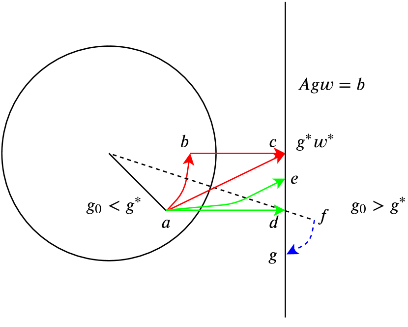
Figure 2: Consider the function $f(w_{1},w_{2},g)$ with $A=a\in\mathbb{R}^{1\times 2}$. Then GD converges to $d$, while rPGD and WN could result in a point ($e$ or $c$) closer to minimum norm $c$ depending on the stepsize schedule of $g$. Part I in Theorem 2.6 suggests that rPGD and WN will follow the path $a\to e$ if $\gamma_{t}$ and $\eta_{t}$ converge to zero at the same rates, and Part II implies the red path $a\to b\to c$ to the minimum norm solution (if $g_{0}$ is fixed for a certain time, and updated later). The optimal path $a\to c$ is taken when $g$ is updated in a careful way. On the other hand, starting with $g_{0}>g^{*}$, for instance at $f$, (7) shows the limit is $g$, further away from $g^{*}w^{*}$.

A Concrete Example. To gain more insight, we provide here a simple example (see also Figure 2). Suppose we have a two-dimensional parameter $w$, and we make a 1-dimensional observation using the matrix $A=[1,0]$, and $y=1$. Then, the equation we are solving is $gw[1]=1$ (where square brackets index coordinates of vectors), and the minimum norm solution is $w=[1,0]^{\top}$, with $g^{*}=1$. Our results guarantee that the WN flow converges to either (1) a zero of the loss, or (2) to a stationary point such that $g=0$ and $w^{\top}A^{\top}y=0$. The second condition reduces to $w[1]\cdot y=0$. Now, if $y\neq 0$ (which is the typical case), then this reduces to $w[1]=0$, and since $\|w\|=1$, we have two solutions $w[2]=\pm 1$. So this leads to two spurious stationary points $(g,w)=(0,[0,\pm 1]^{\top})$, which are not global minima. The loss value at these points is $1$, and so if we start at any point such that the loss is less than one, then we converge to a global mininum. If $y=0$, then this leads to infinitely many stationary points, i.e. all of those with $g=0$, but these turn out to be global minima.

Suppose moreover that we start with $w_{0}=[0,1]^{\top}$ and set $c=1$. Suppose now that we start with some $g_{0}\neq 0$. Then WN flow converges to a solution $gw=[1,\exp([g_{0}^{2}-1]/2)]^{\top}.$ If $g_{0}$ is relatively small, this quantity is close to $x^{*}=[1,0]^{\top}$, closer than the gradient flow solution $[1,1]$.

3 Discrete Time Analysis

In this section, we switch to discrete time. It turns out that analyzing rPGD is more tractable than WN, so we will focus on rPGD. Since the two algorithms collapse to the same flow in continuous time, their dynamics should be “close" in finite time, especially in the small stepsize regime. We show that rPGD with properly chosen learning rates converges close to the min norm solution even when the initialization is far away from the origin. We study rPGD based on the intuition that $\|w_{t}^{\perp}\|$ decreases after the normalization step.

Orthogonal Data Matrix.

Consider first the simple case where the feature matrix $A$ has orthonormal rows, i.e., $AA^{\top}=I$. Our strategy for rPGD to reach the minimum $\ell_{2}$-norm solution is to use the optimal stepsize for $w$ and a small stepsize for $g$ such that $g_{t}^{2}<g^{*2}$ for all iterations. The key intuition is that with a small stepsize, the loss stays positive and ensures the direction $w_{t}$ has sufficient time to find $w^{*}$. On the contrary, if we use a large stepsize for $g$, then it is possible for $g_{t}$ to be greater than $g^{*}$ so that $w_{t}$ can potentially converge to the wrong direction.

Condition 3.1.

(Two-stage learning rates) We update $w$ with its optimal step-size $\eta_{t}=1/g_{t}^{2}$. For the stepsize of $g_{t}$, we use two constant values: (a) $\smash{\gamma_{t}=\gamma^{(1)}}$ when $0\leq t\leq T_{1}$; (b) $\smash{\gamma_{t}=\gamma^{(2)}}$ when $t\geq T_{1}+1$, for a $T_{1}$ specified below.

Theorem 3.2 (Convergence for Orthogonal Matrix $A$).

Suppose the initialization satisfies $0<g_{0}<g^{*}$, and that $w_{0}$ is a vector with $\|w_{0}\|=1$. Let $\delta_{0}=(g^{*})^{2}-(g_{0})^{2}$. Set an error parameter $\varepsilon>0$ and the stepsize given in Condition 3.1 with a hyper-parameter $\rho\in(0,1]$ for $\gamma^{(1)}$. Running the rPGD algorithm, we can reach $\|w_{T_{1}}^{\perp}\|\leq\varepsilon$ and $g_{T_{1}}^{2}\leq g^{*2}-\rho\delta_{0}$ after $T_{1}$ iterations, and $\|w_{T}^{\perp}\|\leq\varepsilon$ and $\|Ag_{T}w_{T}-b\|^{2}\leq 3\varepsilon g^{*2}$ after $T=T_{1}+T_{2}$ iterations, if we set stepsizes as follows.

• Set $\gamma^{(1)}=\mathcal{O}\left(\frac{\rho}{\log(1/\varepsilon)}\left(\frac{g_{0}}{g^{*}}\right)^{2}\log\left((1-\rho)\frac{g^{*}}{g_{0}}+\rho\right)\right)$ and $\gamma^{(2)}\leq\frac{1}{4}$. Then we have

  $$T_{1}=\mathcal{O}\left(\frac{(g^{*})^{2}}{\rho\delta_{0}}\log\left(\frac{1}{\varepsilon}\right)\right);\quad T_{2}=\mathcal{O}\left(\frac{1}{\gamma^{(2)}}\log\left(\frac{(\rho\delta_{0}/g^{*2})^{2}}{\varepsilon}\right)\right).$$

• Set $\gamma^{(1)}=0$ and $\gamma^{(2)}<\frac{1}{4}$. Then we have

  $$T_{1}=\mathcal{O}\left(\frac{g_{0}^{2}}{\delta_{0}}\log\left(\frac{1}{\varepsilon}\right)\right);\quad T_{2}=\mathcal{O}\left(\frac{1}{\gamma^{(2)}}\log\left(\frac{\sqrt{\delta_{0}/g^{*2}}}{\varepsilon}\right)\right).$$

We restate the theorem with the explicit forms of $T_{1}$ and $T_{2}$, along with the proof, in Appendix E.1 and E.2. The theorem requires knowing $g^{*}$, which can be approximated by $\|y\|$ (as $g^{*}=\|y\|$). When all parameters other than $\varepsilon$ are treated as constants, this shows that rPGD converges to the minimum norm solution with the same rate $\log(1/\varepsilon)$ as standard GD starting from the origin. However, the constants in front the $\log(1/\varepsilon)$ can be large: e.g., in case (a), $(g^{*})^{2}/\rho\delta_{0}$ can be $\gg 1$ if $\rho$ is small or if $|g_{0}|/|g^{*}|\approx 1$. This first $T_{1}$ iterations allow $w_{t}$ to "find" $w^{*}$, while the remaining $T_{2}$ allow $g_{t}$ to converge to $g^{*}$. Both cases show an intrinsic tradeoff between $T_{1}$ and $T_{2}$: a larger $\delta_{0}$ (being far from $g^{*}$) leads to faster convergence in the first phase for $\smash{\|w_{t}^{\perp}\|}$ (i.e. smaller $T_{1}$), but slower convergence in $g_{t}$ and loss (i.e. larger $T_{2}$). Specifically, notice that $\delta_{0}$ is in the denominator of $T_{1}$ but in the numerator of $T_{2}$.

Our proof shows that $g_{t}$ is always increasing for any $g_{0}>0$ (c.f. Lemma E.4). Moreover, $\|w_{t}^{\perp}\|$ decreases at a geometric rate, $\|w_{t+1}^{\perp}\|^{2}\leq({g_{t}^{2}}/{g^{*2}})\|w_{t}^{\perp}\|^{2}$, as long as $|g_{t}|$ is not too close to $|g^{*}|$ (c.f. Lemma E.6 or Equation (15)). This is why the condition $g_{T_{1}}^{2}\leq g^{*2}-\rho\delta_{0}$ is needed, ensuring that $g_{t}$ is far away from $g^{*}$ in all steps before $T_{1}$. This is also why we require a stepsize for $g_{t}$ of order $1/\log(1/\varepsilon)$ (c.f. Equation 16), which is smaller than the constant stepsize in usual GD. Here $\rho$ leads to a tradeoff between $T_{1}$ and $T_{2}$: a smaller $\rho$ results in larger $T_{1}$ but smaller $T_{2}$, vice versa. When $\rho\approx\varepsilon$, we have $T_{1}=\mathcal{O}(1/\varepsilon)$ up to log factors, (a slower rate) and $T_{2}=\mathcal{O}\left(1\right)$. A constant order $\rho$ leads to a faster $\log(1/\varepsilon)$ rate. However, we choose to state the result for the entire range of $\rho\in(0,1]$ for completeness. When $\rho=1$, the stepsize $\gamma^{(1)}$ becomes zero, hence $g_{t}$ does not change. In this case, we can get a stronger result for $T_{1}$ (stated in (b)) using a slightly different method of proof, improving the bounds of case (a) respectively with a factor of $(g^{*}/g_{0})^{2}>1$ for $T_{1}$.

We remark that for orthogonal $A$ with the optimal stepsize ($1/g_{t}^{2}$) for $w_{t}$ and $g_{0}\neq 0$, we have $Aw_{t+1}={Ag^{*}w^{*}}/{(g_{t}\|v_{t}\|)}\neq 0$ (c.f. Lemma E.2). Thus we can escape the saddle points and reach the global minimum, unlike in continuous time where we can be stuck at the stationary points $\mathcal{S}$.

We reiterate that our motivation is not to outperform other methods (e.g. GD starts from zero) in search of the minimum norm solution, but to characterize the regularization effect of weight normalization and shed light on the empirical observation that fixing the scalar $g$ and only optimizing the directions $w$ in training the last layer of neural networks can improve generalization (Goyal et al., 2017; Xu et al., 2019). This is, to our knowledge, the first kind of theory on how to control the learning rates of parameters in weight normalization such as to converge to minimum norm solutions for initialization not close to origin, which may have beneficial generalization properties.

General Data Matrix.

Inspired by the analysis for orthogonal $A$, we now study general data matrices. As we have seen from the orthogonal $A$ case, the stepsize for the scale parameter should be extremely small or even $0$ to make $\|w_{t}^{\perp}\|$ small. Thus, for simplicity, we focus on fixing $g:=g_{0}$ and update only $w$ using rPGD so that the orthogonal component $w^{\perp}$ decreases geometrically until $\|w_{T_{1}}^{\perp}\|\leq\varepsilon$. In addition, we notice from the analysis in Theorem 3.2 that updating $g_{t}$ and $w_{t}$ separately after $t>T_{1}$ (i.e., reaching small $\smash{\|w_{t}^{\perp}\|}$) shows no advantage over GD using $x=gw$. Thus, the best strategy to find $g^{*}w^{*}$ is to use rPGD only updating $w_{t}$ (so $g_{t}=g_{0}<g^{*}$) and then apply standard GD after $T_{1}$ once we have $\|w_{T_{1}}^{\perp}\|\leq\varepsilon$. We focus on the complexity of $T_{1}$ in the remainder, as the remaining steps are standard GD, which is well understood.

Even though we fix $g$, the problem is still non-convex because the projection is on the sphere (rather than the ball), a non-convex surface. However, suppose we can ensure that after each update, the gradient step $v_{t}=w_{t}-\eta_{t}\nabla_{w}f(w_{t},g_{t})$ has norm $\|v_{t}\|\geq 1$. Then the following two constrained non-convex problems are equivalent:

$$\min_{w\in\mathbb{R}^{d}}\|Ag_{0}w-y\|^{2}\text{ s.t. }w\in\{w,\|w\|=1\}\quad\Leftrightarrow\quad\min_{w\in\mathbb{R}^{d}}\|Ag_{0}w-y\|^{2}\text{ s.t. }w\in\{w,\|w\|\leq 1\}$$

Thus our analysis will focus on showing that $\|v_{t}\|\geq 1$. Note that, without loss of generality we can always scale $A$ so that its largest singular value is one.

Proposition 3.3 (General Matrix $A$).

Fix $\delta>0$, and fix a full rank matrix $A$ with $\lambda_{\max}(AA^{\top})=1$. With a fixed $g=g_{0}$ satisfying $g_{0}\leq[g^{*}\lambda_{\min}(AA^{\top})]/(2+\delta)$, we can reach a solution with $\|w_{T_{1}}^{\perp}\|\leq\varepsilon$ in a number of iterations

$$T_{1}=\log\left(\frac{\|w_{0}^{\perp}\|}{\varepsilon}\right)/\log(1+\delta).$$

The proof is in Appendix E.3. The proposition implies that if we set a small $g_{0}=\mathcal{O}(g^{*}\lambda_{\min}(AA^{\top}))$ for general $A$ and $w^{*}$, running rPGD with fixed $g_{0}$ helps regularize the iterates. After starting from $w_{T_{1}}$, we can converge close to the minimum norm solution using standard GD. If the eigenvalues of $A$ are "not too spread out", we can get a better condition for $g_{0}$ using concentation inequalities for eigenvalues. See inequality (46) in Proposition E.9 for more details.

4 Discussion

Limitation of our work. It is important to recognize the limitations of our work. First, our theoretical work only addresses weight normalization (not batch, layer, instance or other normalization methods), and only concerns the setting of linear least squares regression. While this may seem limiting, it is still significant: even in this setting, the problem is not understood, and leads to intriguing insights. In fact there is some recent work on Neural Tangent Kernels arguing overparametrized NNs can be equivalent to linear problems, see e.g., (Jacot et al., 2018; Du et al., 2018; Lee et al., 2019), etc. Second, the continuous limit is only an approximation; however it leads to elegant and interpretable results, which are moreover also reflected in simulations. Third, some of our results concern a two-stage algorithm where the scale is fixed for the first stage; nevertheless, our results on the standard “one-stage" algorithm in continuous time suggest such discrete-time results extend to the situation where the scale is not fixed, but slowly-varying for the first stage.

Related Work. While there is a large literature on weight normalization and implicit regularization (see Sec 4), our work differs in crucial ways. We study the overparametrized case and characterize the implicit regularization for a broad range of initializations (unlike works that study initialization with small norm). Also, we prove convergence and characterize the solution explicitly (unlike works such as (Gunasekar et al., 2018) that assume convergence to minimizers). Below we can only discuss a small number of related works.

Implicit regularization. It has been recognized early that optimization algorithms can have an implicit regularization effect, both in applied mathematics (Strand, 1974), and in deep learning (Morgan and Bourlard, 1990; Neyshabur et al., 2014). It has been argued that “algorithmic regularization" can be one of the main differences between the perspectives of statistical data analysis and more traditional computer science (Mahoney, 2012).

Theoretical work has shown that gradient descent is a form of regularization for exponential-type losses such as logistic regression, converging to the max-margin SVM for separable data (Soudry et al., 2018; Poggio et al., 2019), as well as for non-separable data (Ji and Telgarsky, 2019). Similar results have been obtained for other optimization methods (Gunasekar et al., 2018), as well as for matrix factorization (Gunasekar et al., 2017; Arora et al., 2019), sparse regression (Vaškevičius et al., 2019), and connecting to ridge regression (Ali et al., 2018). For instance, (Li et al., 2018) showed that GD with small initialization and small step size finds low-rank solutions for matrix sensing. There have also been arguments that neural networks perform a type of self-regularization, some connecting to random matrix theory (Martin and Mahoney, 2018; Mahoney and Martin, 2019). Popular methods for regularization include weight decay (a.k.a., ridge regression) (Dobriban and Wager, 2018; Liu and Dobriban, 2019), dropout (Wager et al., 2013), data augmentation (Chen et al., 2019), etc.

Convergence of normalization methods. (Salimans and Kingma, 2016) argued that their proposed weight normalization (WN) method, optimizing $x=gw/\|w\|_{2}$ over $g\geq 0$ and $w\in\mathbb{R}^{d}$, increases the norm of $w$, and leads to robustness to the choice of stepsize. (Hoffer et al., 2018) studied normalization with weight decay and learning-rate adjustments. (Du et al., 2018) proved that GD with WN from randomly initialized weights could recover the right parameters with constant probability in a one-hidden neural network with Gaussian input. (Ward et al., 2019) connected the WN with adaptive gradient methods and proved the sub-linear convergence for both GD and SGD. (Cai et al., 2019) showed that for under-parametrized least squares regression (which is different from our over-parametrized setting), batch normalized GD converges for arbitrary learning rates for the weights, with linear convergence for constant learning rate. Similar results for scale-invariant parameters can be found in (Arora et al., 2018) with more general models, extending to the non-convex case. (Kohler et al., 2019) proved linear convergence of batch normalization in halfspace learning and neural networks with Gaussian data, using however parameter-dependent learning rates and optimal update of the length $g$. (Luo et al., 2019) analyzed batch normalization by using a basic block of neural networks and concluded that batch normalization has implicit regularization. (Dukler et al., 2020) discussed the convergence of two-layer ReLU network with weight normalization under the NTK regime. However, none of the above give the invariants we do.

Nonlinear Least Mean Squares (NLMS) . Normalization methods are possibly related to the Nonlinear Least Mean Squares (NLMS) methods from signal processing (see e.g. Proakis, 2001; Haykin and Widrow, 2002; Haykin, 2005; Hayes, 2009). NLMS can be viewed as an online algorithm where the samples $a_{t},y_{t}$ ($a_{t}$ are the rows of $A$, $y_{t}$ are the entries of $y$) arrive in an online fashion, and we update the iterates as $x_{t+1}=x_{t}-\eta r_{t}a_{t}/\|a_{t}\|^{2}$, where $r_{t}=y_{t}-x_{t}^{\top}a_{t}$ are the residuals. There is a connection to randomized Kaczmarcz methods Strohmer and Vershynin (2009). However, it is not obvious how they are related to weight normalization or rPGD/WN, e.g., these methods are under online setting, while rPGD/WN are offline.

Broader Impact

Our work is on the foundations and theory of machine learning. One of the distinctive characteristics of contemporary machine learning is that it relies on a large number of "ad hoc" techniques, that have been developed and validated through computational experiments. For instance, the optimization of neural networks is in general a highly nonconvex problem, and there is no complete theoretical understanding yet as to how exactly it works in practice. Moreover, there a large number of practical "hacks" that people have developed that help in practice, but lack a solid foundation. Our work is about one of these techniques, weight normalization. We develop some nontrivial theoretical results about it in a simplified "model". This work does not directly propose any new algorithms. But we hope that our work will have an impact in practice, namely that it will help practitioners understand what the WN method is doing (important, as people naturally want to understand and know "why" things work), and possibly in the future, help us develop better algorithms (here the principle being that "if you understand it you can improve it", which has been useful in engineering and computer science for decades).

Appendix A Adaptive Regularization

We illustrate that the two Algorithms can heuristically be viewed as GD on adaptively $\ell_{2}$-regularized regression problems. The regularization parameter changes for each iteration in the algorithms:

$$\min_{x_{t+1}}\left(\frac{1}{2}\|Ax_{t+1}-Ax^{*}\|^{2}+\lambda(w_{t},g_{t},\eta,A,y)\|x_{t+1}\|^{2}\right).$$

However, it is difficult to characterize the behavior of $\lambda_{t}$ in general.

WN. Let $x_{t}=\frac{g_{t}w_{t}}{\|w_{t}\|}$. Notice that:

$$\frac{g_{t+1}w_{t+1}}{\|w_{t+1}\|}= \frac{g_{t}}{\|w_{t}\|}w_{t}+(\frac{g_{t+1}}{\|w_{t+1}\|}-\frac{g_{t}}{\|w_{t}\|})w_{t}-\eta_{t}\frac{g_{t+1}}{\|w_{t+1}\|}\frac{g_{t}}{\|w_{t}\|}(I-\frac{w_{t}w_{t}^{T}}{\|w_{t}\|^{2}})A^{T}r$$

This can be translated to the update of $x_{t}$ as

$$x_{t+1}= x_{t}-\eta_{t}\frac{g_{t+1}g_{t}}{\|w_{t+1}\|\|w_{t}\|}A^{T}r-\left(1-\frac{g_{t+1}\|w_{t}\|}{g_{t}\|w_{t+1}\|}-\eta_{t}\frac{g_{t+1}}{\|w_{t+1}\|}\langle\frac{w_{t}}{\|w_{t}\|^{2}},A^{T}r\rangle\right)x_{t}$$

rPGD. Let $x_{t}=g_{t}w_{t}$. The update of $w_{t}$ in Algorithm 2 is

$$w_{t+1}=\frac{1}{\|v_{t}\|}(w_{t}-\eta_{t}g_{t}A^{T}(Ax_{t}-Ax^{*})).$$ (8)

We can now write the update of $x_{t+1}=g_{t+1}w_{t+1}$ as

$$x_{t+1}=x_{t}-\frac{\eta_{t}g_{t}g_{t+1}}{\|v_{t}\|}A^{T}(Ax_{t}-Ax^{*})-(1-\frac{g_{t+1}}{g_{t}\|v_{t}\|})x_{t}.$$

Both updates can be viewed as a gradient step on the following $\ell_{2}$-regularized regression problem, with specific choices of $\lambda_{t}$ at iteration $t$:

$$\frac{1}{2}\|Ax_{t+1}-Ax^{*}\|^{2}+\lambda_{t}\|x_{t+1}\|^{2},$$

We see that the regularization parameter changes for each iteration for both WN and rPGD, as follows:

$$\text{(WN)}\quad\lambda_{t}= \frac{\|w_{t+1}\|\|w_{t}\|}{g_{t+1}g_{t}}(1-\frac{g_{t+1}\|w_{t}\|}{g_{t}\|w_{t+1}\|}-\eta\frac{g_{t+1}}{\|w_{t+1}\|}\langle\frac{w_{t}}{\|w_{t}\|^{2}},A^{T}r\rangle)$$

$$\text{(rPGD)}\quad\lambda_{t}= (g_{t}\|v_{t}\|-g_{t+1})/(\eta_{t}g_{t}^{2}g_{t+1}).$$

The regularization parameter $\lambda_{t}$ is highly dependent on $g_{t}$, $g_{t+1}$ and the input matrix $A$. However, it is difficult to characterize the behavior of $\lambda_{t}$ in general. In particular, we require the parameters $g_{t}$, $g_{t+1}$, $w_{t}$ and $w_{t+1}$ updated in a way that $\lambda_{t}>0$. For the simpler setting of orthogonal $A$, we can see for rPGD that: 1) If the learning rate of $g$ is small enough, we will have $g_{t+1}<g_{t}\|v_{t}\|$, which means that $\lambda_{t}>0$; 2) When $g_{t}w_{t}$ is close to $g^{*}w^{*}$, we will have $\|v_{t}\|\approx 1$, and $g_{t+1}\approx g_{t}$, which means that $\lambda_{t}\approx 0$.

Appendix B Proof of Lemma 2.2

Proof.

rPGD. First we start with the reparametrized Projected Gradient Descent algorithm. The gradients for rPGD are

$$\nabla_{w}f(w,g)=g\nabla L(gw),\;\nabla_{g}f(w,g)=w^{T}\nabla L(gw),$$

First, the gradient step on $g$ clearly leads to the gradient flow for $g$. Second, for the update on $w$, we expand all terms to first order in $\eta$. Let $a_{t}=\nabla_{w_{t}}f(w_{t},g_{t})$. We start by expanding the squared Euclidean norm

$$\|w_{t}-\eta\nabla_{w_{t}}f(w_{t},g_{t})\|_{2}^{2} =\|w_{t}-\eta a_{t}\|_{2}^{2}$$

$$=\|w_{t}\|^{2}-2\eta w_{t}^{\top}a_{t}+\eta^{2}\|a_{t}\|_{2}^{2}$$

$$=1-2\eta w_{t}^{\top}a_{t}+O(\eta^{2}).$$

On the last line, we have used that the iterates are normalized, so $\|w_{t}\|^{2}=1$.

Now, we can use the expansion $(1+x)^{1/2}=1+x/2+O(x^{2})$, valid for $|x|\ll 1$, on the right hand side of the above display, to get

$$\|w_{t}-\eta\nabla_{w_{t}}f(w_{t},g_{t})\|_{2} =1-\eta w_{t}^{\top}a_{t}+O(\eta^{2}).$$

Next we use this expansion in the update rule for the weights:

$$w_{t+1}=\frac{w_{t}-\eta\nabla_{w_{t}}f(w_{t},g_{t})}{\|w_{t}-\eta\nabla_{w_{t}}f(w_{t},g_{t})\|_{2}}$$

$$=\frac{w_{t}-\eta a_{t}}{1-\eta w_{t}^{\top}a_{t}+O(\eta^{2})}$$

$$=(w_{t}-\eta a_{t})\cdot(1+\eta w_{t}^{\top}a_{t}+O(\eta^{2})).$$

In the last line, we have used the expansion

$$\frac{1}{1-\eta x+O(\eta^{2})} =1+\eta x+O(\eta^{2})$$

valid for $|\eta|\ll 1$ and $x$ of a constant order. Recall now that for an arbitrary vector $w$, we defined $P_{w^{\perp}}=I-\frac{ww^{\top}}{\|w\|_{2}^{2}}$ as the projection into the orthocomplement of $w$. Since $\|w_{t}\|=1$, we have $\mathcal{P}_{t}=I-w_{t}w_{t}^{\top}$. By expanding the product and rearranging, keeping only the terms of larger order than $\eta$, we find

$$w_{t+1}=w_{t}-\eta a_{t}+\eta w_{t}w_{t}^{\top}a_{t}+O(\eta^{2})$$

$$=w_{t}-\eta\mathcal{P}_{t}a_{t}+O(\eta^{2}).$$

Taking $\eta\to 0$ and substituting the expression for $a_{t}$ and $\nabla_{w}f(w,g)$, we obtain the rPGD flow dynamics for $w$, i.e., $\dot{w}_{t}=-g_{t}\mathcal{P}_{t}\nabla L(g_{t}w_{t})$. The update rule for $g$ follows directly.

WN. We now study weight normalization Salimans and Kingma [2016]. The WN objective function can be written using the loss function $L(x)=\|Ax-y\|^{2}/2$ as

$$h(g,w)=L\left(g\frac{w}{\|w\|}\right).$$

The discrete time algorithm is thus updated as

$$v_{t} =w_{t}/\|w_{t}\|$$

$$r_{t} =y-g_{t}Av_{t}$$

$$g_{t+1} =g_{t}-c\eta\cdot\langle{v_{t},\nabla L\left(g_{t}\frac{w_{t}}{\|w_{t}\|}\right)\rangle}$$

$$w_{t+1} =w_{t}-\eta\cdot g_{t}\cdot\mathcal{P}_{t}\frac{1}{\|w_{t}\|}\nabla L(g_{t}\frac{w_{t}}{\|w_{t}\|}).$$

When $\eta\to 0$, we recover the gradient flow on $g_{t}$ and $w_{t}$, i.e., recalling $v_{t}=w_{t}/\|w_{t}\|$

$$\dot{g}_{t} =-c\cdot\langle{v_{t},\nabla L(g_{t}v_{t})\rangle}$$

$$\dot{w}_{t} =-g_{t}\cdot\mathcal{P}_{t}\frac{1}{\|w_{t}\|}\nabla L(g_{t}v_{t})=-\frac{g_{t}}{\|w_{t}\|}\cdot\mathcal{P}_{t}\nabla L(g_{t}v_{t}).$$

Note the fact $\frac{d\|w_{t}\|^{2}}{dt}=2w_{t}^{T}\dot{w}_{t}=0$ which gives $\|w_{t}\|=\|w_{0}\|=1$.

Hence, for WN with initialization $\|w_{0}\|=1$, we have that $g_{t},v_{t}$ evolves exactly equivalent to the rPGD flow. The final formula for WN and rPGD that we will analyze is:

$$\dot{g}_{t} =-c\cdot w_{t}^{T}A^{T}r_{t}$$

$$\dot{w}_{t} =-g_{t}\cdot\mathcal{P}_{t}A^{T}r_{t}.$$

∎

Appendix C Remaining Proofs for Section 2

C.1 Proof of Lemma 2.3

Proof.

At a stationary points of the loss, we have, with $r=y-Agw$

$$\partial_{g}h(w,g) =w^{T}A^{T}r=0$$

$$\partial_{w}h(w,g) =g\cdot P_{w^{\perp}}A^{T}r=0.$$

If $g\neq 0$, then we get $P_{w^{\perp}}A^{T}r=0$. By adding this up with the first equation, we get $A^{T}r=0$. Using that the smallest eigenvalue of $AA^{T}$ is nonzero, we conclude that $r=0$. Hence this is stationary point with zero loss, which is also a global minimum.

Else, if $g=0$, we see that $r=y-Agw=y$. Hence in this case, the stationary points belong to the set $S:=\{(g,w):g=0,y^{T}Aw=0\}.$ This finishes the proof. ∎

C.2 Proof of Lemma 2.4 (dynamics of loss $\|r_{t}\|$)

We have

$$d[1/2\|r_{t}\|^{2}]/dt =r_{t}^{T}\dot{r}_{t}=r_{t}^{T}Ad(g_{t}w_{t})/dt$$

$$=r_{t}^{T}A[\dot{g}_{t}w_{t}+g_{t}\dot{w}_{t}]$$

$$=-r_{t}^{T}A[c\cdot w_{t}w_{t}^{T}A^{T}r_{t}+g_{t}^{2}\mathcal{P}_{t}A^{T}r_{t}]$$

$$=-r_{t}^{T}A[c\cdot w_{t}w_{t}^{T}+g_{t}^{2}\mathcal{P}_{t}]A^{T}r_{t}$$

Thus,

$$d[1/2\|r_{t}\|^{2}]/dt\leq-\min\{g_{t}^{2},c\}\|A^{T}r_{t}\|^{2},\quad d[1/2\|r_{t}\|^{2}]/dt\geq-\max\{g_{t}^{2},c\}\|A^{T}r_{t}\|^{2}.$$

We get a geometric convergence of the loss to zero, as soon as we can get a lower bound on $g_{t}^{2}$, which will be discussed below. If we have $g_{t}^{2}\geq C^{2}$ for some constant $C^{2}>0$, we have

$$\min(g_{t}^{2},c)r_{t}^{T}AA^{T}r_{t}\geq\min(C^{2},c)\lambda_{\min}(AA^{T})\|r_{t}\|^{2}$$

and so with $k:=\min(C^{2},c)\lambda_{\min}(AA^{T})$,

$$d[1/2\cdot\|r_{t}\|^{2}]/dt \leq-k\|r_{t}\|^{2}\quad\Rightarrow\quad\|r_{t}\|^{2}\leq\exp(-kt)\|r_{0}\|^{2}.$$

C.3 Proof of Lemma 2.5

Define $P^{\perp}$ the projection into the orthocomplement of the row span of $A$, hence $w^{\perp}=P^{\perp}w$ and $P^{\perp}A^{T}=0$. For simplicity, write $h(w_{t},g_{t})=h_{t}$

$$\begin{split}\frac{d{w_{t}^{\perp}}}{dt}&=P^{\perp}\frac{d{w_{t}}}{dt}=-\frac{g_{t}}{\left\|w_{t}\right\|}P^{\perp}(I-\frac{w_{t}w_{t}^{\top}}{\left\|w_{t}\right\|^{2}})\nabla_{w}h_{t}=\frac{g_{t}}{\left\|w_{t}\right\|}P^{\perp}\frac{w_{t}w_{t}^{\top}}{\left\|w_{t}\right\|^{2}}\nabla_{w}h_{t}=\frac{g_{t}}{\left\|w_{t}\right\|^{2}}P^{\perp}{w_{t}}\left(\nabla_{g}h_{t}\right)\\ &=-\frac{g_{t}}{\left\|w_{t}\right\|^{2}}P^{\perp}{w_{t}}\left(\frac{1}{c}\frac{dg_{t}}{dt}\right)=-\frac{1}{2}\frac{P^{\perp}{w_{t}}}{\left\|w_{t}\right\|^{2}c}\frac{dg^{2}_{t}}{dt}=-\frac{1}{2}\frac{w_{t}^{\perp}}{\left\|w_{0}\right\|^{2}c}\frac{dg^{2}_{t}}{dt}.\end{split}$$

The last equality due to the fact that ${d\|w_{t}\|^{2}}/{dt}=2w_{t}^{T}\dot{w}_{t}=0$, which is also observed in [Tian et al., 2019, Tian, 2019]. Solving the dynamics $\frac{d{w_{t}^{\perp}}}{dt}=-\frac{1}{2}\frac{w_{t}^{\perp}}{c\left\|w_{0}\right\|^{2}}\frac{dg^{2}_{t}}{dt}$ with $\|w_{0}\|=1$ results in (6).

C.4 Proof of Theorem 2.6 (Convergence in the general case)

C.4.1 Proof that either the loss converges to zero, or the iterates $(g_{t},w_{t})$ converge to the stationary set $\mathcal{S}$ defined in Lemma 2.3.

We start with the ODE for the loss,

$$d[1/2\|r_{t}\|^{2}]/dt =-r_{t}^{T}A[c\cdot w_{t}w_{t}^{T}+g_{t}^{2}\mathcal{P}_{t}]A^{T}r_{t}.$$ (9)

This shows that the loss is decreasing, possibly not strictly.

If we have $g_{t}^{2}$ bounded away from zero, then the loss converges to zero geometrically. Thus, the only remaining case is when $g_{t}\to 0$.

Now, we have that the iterates take the form $x_{t}=g_{t}w_{t}$, and $\|w_{t}\|=1$ are bounded. Hence, as $g_{t}\to 0$, we must have $x_{t}\to 0$.

Since the loss is continuous, we also have $\|r_{t}\|^{2}=\|y-Ag_{t}w_{t}\|^{2}\to\|y\|^{2}$.

Suppose that the loss does not converge to zero. Since the loss is decreasing, this means that $\|r_{t}\|\to c>0$ for some constant $c$.

From Equation (9), this implies that

$$(r_{t}^{T}Aw_{t})^{2} \to 0.$$

Else, if this quantity is bounded away from zero, then $d[1/2\|r_{t}\|^{2}]/dt<-c^{\prime}$ for some $c^{\prime}>0$, which would show $\|r_{t}\|$ decreases unboundedly, and is a contradiction.

Thus, we conclude that if the residual $r_{t}$ does not converge to zero, then the iterates $x_{t}=g_{t}w_{t}$ converge to zero: $x_{t}\to 0$. Moreover, $g_{t}\to 0$ and $y^{T}Aw_{t}\to 0$. Given that $w_{t}$ is bounded, this shows that $(g_{t},w_{t})$ converges to the set of those stationary points of the loss characterized by

$$S:=\{(g,w):g=0,y^{T}Aw=0\}.$$

Note specifically that we have not shown that $w_{t}$ converges to a specific stationary point, but rather only that it converges to the set $S$ of stationary points given above.

This result does not give a rate of convergence, so it is weaker than the result when $g_{t}$ is bounded away from zero. However, it is also more general. Initializing such that the loss is less than the loss at zero can be achieved conveniently, because we can calculate the value of the loss.

C.4.2 Part I: Characterizing the solution when $c>0$

The characterization follows by tracking the dynamics of the components in the row span of $A$ and its orthocomplement separately. The component in the row span converges to $x^{*}$. The normalized component $w_{t}^{\perp}$ in the orthocomplement is characterized by the invariant from the prior lemma. The scale of that component converges to $g^{*}$, as $g_{t}\to g^{*}$. This gives the desired result.

C.4.3 Part II: Fixed $g_{t}$, i.e. $c=0$

For the fixed $g_{t}$ case, we have

$$d[1/2\cdot\|r_{t}\|^{2}]/dt =r_{t}^{T}\dot{r}_{t}=r_{t}^{T}Ad(g_{t}w_{t})/dt$$

$$=r_{t}^{T}A[\dot{g}_{t}w_{t}+g_{t}\dot{w}_{t}]$$

$$=r_{t}^{T}Ag_{0}\dot{w}_{t}$$

$$=-r_{t}^{T}Ag_{0}\mathcal{P}_{t}g_{0}A^{T}r_{t}$$

$$=-g_{0}^{2}\|\mathcal{P}_{t}A^{T}r_{t}\|^{2}.$$

Now, it follows that $\|r_{t}\|$ is a non-increasing quantity, which is also strictly decreasing as long as $\|\mathcal{P}_{t}A^{T}r_{t}\|>0$. It also follows that as $t\to\infty$, we have $\|\mathcal{P}_{t}A^{T}r_{t}\|\to 0$. Now, since $g_{0}<g^{*}$, it follows that $A^{T}r_{t}$ has a norm that is strictly bounded away from zero, i.e., $\|A^{T}r_{t}\|>c_{0}>0$ for some $c_{0}>0$. So, we do not have the residual going to zero in this case. Hence, this can also be written as $w_{t}=c_{t}\cdot A^{T}r_{t}/\|A^{T}r_{t}\|$, for some sequence of scalars $c_{t}$ with $\liminf c_{t}^{2}>0$.

Hence, $w_{t}$ becomes asymptotically parallel to the row space of $A$. Now, since $w_{t}$ lives on the compact space of unit vectors, considering any subsequence of it, it also follows that it has a convergent subsequence. Let $w$ be the limit along any convergent subsequence. It follows that $w=\pm A^{T}r/\|A^{T}r\|$. Next we note that the solution with $+$ actually maximizes the loss over $\|w\|=1$. Hence, the only possible solution is $w=-A^{T}r/\|A^{T}r\|$. Since this holds for any convergent subsequence, it follows that $w_{t}$ itself must converge.

Now we get a more explicit form for the solution $w$. We can say that $w$ is the unique unit norm vector such that $w=-\hat{c}A^{T}r$, for some $\hat{c}>0$. Then we can write that equation as

$$w =-\hat{c}A^{T}(Agw-y)$$

$$(I+cgA^{T}A)w =\hat{c}A^{T}y$$

$$w =(\hat{c}^{-1}I+gA^{T}A)^{-1}A^{T}y.$$

Thus, $w$ is the unique vector of the above form such that $\|w\|=1$. This can be viewed as a form of implicit regularization. Namely, $w$ is the unique vector, for which there is some regularization parameter $\hat{c}$ such that, $w$ minimizes the regularized least squares objective

$$\frac{1}{2}\|Agw-y\|^{2}+\frac{g}{2\hat{c}}\|w\|^{2}$$

and $\|w\|=1$. This $w$ will in general not be the pointing in the direction of the optimal solution. We recall that the optimal solution $w^{*}$ has the form $w^{*}=A^{\dagger}b/\|A^{\dagger}y\|$, where $A^{\dagger}$ is the pseudoinverse of $A$. We recall that the action of the pseudoinverse can be characterized as the limit of ridge regularization with infinitely small penalization, i.e., $A^{\dagger}y=\lim_{\lambda\to 0}(A^{T}A+\lambda I)^{-1}A^{T}y$. For orthogonal $A$, we see that $w$ converges to the right direction, because $A^{T}=A^{\dagger}$. However, for general $A$, the flow does not in general converge to the min-norm direction.

Now, suppose we start the flow for both $g_{t},w_{t}$ again from a point $w_{0}$ that belongs to the span of the row space of $A$ (call it $R$). Then, by the update rule for $w_{t}$, it follows that $w_{t}\in R$ for all $t$. Therefore, the derivative of the loss becomes

$$d[1/2\cdot\|r_{t}\|^{2}]/dt =r_{t}^{T}\dot{r}_{t}=r_{t}^{T}Ad(g_{t}w_{t})/dt$$

$$=r_{t}^{T}A[\dot{g}_{t}w_{t}+g_{t}\dot{w}_{t}]$$

$$=-r_{t}^{T}A[w_{t}w_{t}^{T}A^{T}r_{t}+g_{t}^{2}\mathcal{P}_{t}A^{T}r_{t}]$$

$$=-(r_{t}^{T}Aw_{t})^{2}.$$

From arguments similar to before, it follows that $r_{t}^{T}Aw_{t}\to 0$ as $t\to\infty$. Moreover, from a similar subsequence argument it also follows that $w_{t}\to w$ such that $r^{T}Aw=0$. Since $\|w\|=1$ and $A$ has full row rank, it follows that $r=0$. Hence the flow converges to a zero of the loss. Moreover, since $w\in R$, it follows that this is the minimum norm solution.

C.5 Proof of Theorem 2.7 (Convergence rate)

Note first that by (6), we have

$$g_{t}^{2}=2\log\|w_{0}^{\perp}\|+g_{0}^{2}-2\log\|w_{t}^{\perp}\|\geq 2\log\|w_{0}^{\perp}\|+g_{0}^{2}$$ (10)

where the last inequality is due to the fact $\|w_{t}^{\perp}\|\leq\|w_{t}\|=1$. Thus, we have our lower bound. From Lemma 2.4, we get the convergence rate for this case.

Appendix D Beyond Linear Regression

Here we illustrate that the invariant in the optimization path holds more generally than for linear regression, and specifically for certain general loss functions that only depend on a small dimensional subspace of the parameter space. Let $L:\mathbb{R}^{d}\to\mathbb{R}$ be the loss function, and our goal is to solve

$$\min_{x\in\mathbb{R}^{d}}L(x)$$ (11)

where $L(x)$ is differentiable and satisfies Assumption D.1.

Assumption D.1 (Low-dimensional gradient).

There exists a projection matrix $P\in\mathbb{R}^{d\times d}$ with rank $r<d$ such that

$$(I-P)\nabla L(x)=0,\forall x\in\mathbb{R}^{d}.$$

Let $P^{\perp}=(I-P)$. Assumption D.1 is equivalent to the fact that the gradient of $L$ lives in the low-dimensional space given by the span of $P$, $\nabla L(x)\in span(P)$. This implies

$$L(x)=L(Px)\quad\forall x\in\mathbb{R}^{d}.$$

This means that the objective only depends on the projection of $x$ into the span of $P$. To use the orthogonal projection in what follows, define $x^{\parallel}=Px$ and $x^{\perp}=P^{\perp}x$. For the undetermined linear regression, $P=A^{\dagger}A$ where $A^{\dagger}$ is the pseudo-inverse of the matrix $A$.

Theorem D.2 (WN flow Invariance for General Loss).

Consider the loss function in (11) with Assumption D.1. The WN method transforms the loss function to $h(g,w)=L\left(g_{t}\frac{w_{t}}{\|w_{t}\|}\right)$. The WN gradient flow from Algorithm 1 with initial condition $(w_{0},g_{0})$, started from $w_{0}$ with not necessarily unit norm, has the invariant

$$w_{t}^{\perp}=\exp\left(\frac{g_{0}^{2}-g_{t}^{2}}{2\|w_{0}\|^{2}}\right)w_{0}^{\perp}.$$

The proof of the above theorem is a simple extension of the proof in Part I of Lemma 2.5 with $A^{\top}r_{t}=\nabla L\left(g_{t}\frac{w_{t}}{\|w_{t}\|}\right)$. This result suggests that the reason for the invariance is that the original objective function before reparametrization only depends on a smaller dimensional space.

Appendix E Remaining Proofs for Section 3

E.1 Proof of Theorem 3.2 Case (a)

We restate the case (a) of Theorem 3.2 here.

Theorem E.1 (Updating $g$ in Phase I).

Suppose we initialize with $g_{0}<g^{*}$. Let $\delta_{0}=(g^{*})^{2}-(g_{0})^{2}>0$, $0<\rho<1$ and $\delta<\frac{\varepsilon}{2g^{*}+\varepsilon}$. Suppose the number of iterations $T_{1}$ and $T_{2}$ is of the order:

$$T_{1}=\left(1+\frac{(g^{*})^{2}}{\rho\delta_{0}}\right)\log\left(\frac{1-\|Aw_{0}\|^{2}}{\delta^{2}}\right)=\mathcal{O}\left(\frac{(g^{*})^{2}}{\rho\delta_{0}}\log\left(\frac{1}{\delta^{2}}\right)\right),$$

$$T_{2}=\frac{1}{\gamma^{(2)}}\log\left(\frac{\rho\delta_{0}}{g^{*2}(1-\varepsilon)\sqrt{\varepsilon}}\right)=\mathcal{O}\left(\frac{1}{\gamma^{(2)}}\log\left(\frac{\rho(g^{*2}-g_{0}^{2})}{g^{*2}\sqrt{\varepsilon}}\right)\right).$$

Fix $g_{1}=g_{0}$ at the first step. For iterations $t=1,\ldots,T_{1}-1$, set the stepsize for $g$ to

$$\gamma^{(1)}<\min\left\{\frac{\|Ag_{0}w_{0}\|^{2}}{2T_{1}((g^{*})^{2}-\|Ag_{0}w_{0}\|^{2})}\log\left((1-\rho)\frac{g^{*2}}{g_{0}^{2}}+\rho\right),\frac{1}{2(1+\|Aw_{0}\|^{2})}\right\}$$

and to any $\gamma^{(2)}\leq\frac{1}{4}$ for $t=T_{1},T_{1}+1,\ldots,T_{1}+T_{2}-1$. Set $\eta_{t}=1/g_{t}^{2}$. Then we reach $\|w_{T}^{\perp}\|\leq\varepsilon$ and $\|Ag_{T}w_{T}-b\|^{2}\leq\varepsilon g^{*2}$ after $T=T_{1}+T_{2}$ iterations.

Proof.

The norm $\|w^{\perp}\|$. Let us first get the upper bound of $g_{t+1}$ to see how the norm of $\|w_{t}^{\perp}\|=1-\|Aw_{t}\|^{2}$ evolves. Suppose that we have for some $0<\rho<1$

$$(g^{*})^{2}-\|Ag_{T_{1}}w_{T_{1}}\|^{2}\geq(g^{*})^{2}-g_{T_{1}}^{2}=\rho\delta_{0}$$ (12)

By Lemma E.6, we have

$$\|w_{T_{1}}^{\perp}\|^{2}=(1-\|Aw_{T_{1}}\|^{2}) \leq\exp(-\sum_{i=1}^{T_{1}}\frac{(g^{*})^{2}-\|Ag_{i}w_{i}\|^{2}}{(g^{*})^{2}+(g^{*})^{2}-\|Ag_{i}w_{i}\|^{2}})(1-\|Aw_{0}\|^{2})$$ (13)

$$\leq\exp(-\sum_{i=1}^{T_{1}}\frac{(g^{*})^{2}-\|Ag_{T_{1}}w_{T_{1}}\|^{2}}{(g^{*})^{2}+(g^{*})^{2}-\|Ag_{T_{1}}w_{T_{1}}\|^{2}})(1-\|Aw_{0}\|^{2})$$ (14)

$$\leq\exp(-\frac{\rho\delta_{0}T_{1}}{(g^{*})^{2}+\rho\delta_{0}})(1-\|Aw_{0}\|^{2})$$ (15)

we have $\|w_{T_{1}}^{\perp}\|^{2}=1-\|Aw_{T_{1}}\|^{2}\leq\delta^{2}$ when

$$T_{1}=\left(1+\frac{(g^{*})^{2}}{\rho\delta_{0}}\right)\log\left(\frac{1-\|Aw_{0}\|^{2}}{\delta^{2}}\right).$$

Now we only need to verify condition (12). To see this, notice that we use Lemma E.3:

$$g_{t+1}\leq g_{t}+\frac{\gamma g_{t}}{2}(\|v_{t}\|^{2}-1)\text{ for }t<T_{1}$$

Note $\|v_{t}\|^{2}={g^{*2}}/{(g_{t}^{2}\|Aw_{t+1}\|^{2})}>1$ as $\|Aw_{t+1}\|<1$ and $g^{*2}>g_{t}^{2}$. Thus, even though $g_{t}$ grows with the rate $\gamma^{(1)}(\|v_{t-1}\|^{2}-1)$, we use our choice of $\gamma^{(1)}$ and $g_{t+1}<g^{*}$. In fact, we set $\gamma^{(1)}$ small such that after $T_{1}$ there is a gap between $g^{*}$ and $g_{T_{1}}$. We let the gap satisfies $(g^{*})^{2}-g_{T_{1}}^{2}\geq\rho\delta_{0}$:

$$g_{T_{1}+1}^{2}\leq\prod_{t=1}^{T_{1}+1}\left(1+\frac{1}{2}\gamma^{(1)}(\|v_{t-1}\|^{2}-1)\right)^{2}g_{1}^{2}\overset{(a)}{\leq}\exp\left(\gamma^{(1)}(\|v_{0}\|^{2}-1)T_{1}\right)g_{0}^{2}\overset{(b)}{\leq}(g^{*})^{2}-\rho\delta_{0}$$ (16)

where step $(a)$ due to $g_{1}=g_{0}$ and the that

$$\frac{\|v_{t}\|^{2}}{\|v_{t-1}\|^{2}}\leq\frac{g_{t-1}^{2}}{g_{t}^{2}}\leq 1$$ (17)

which is due to $g_{t}^{2}\|v_{t}\|^{2}-g_{t-1}^{2}\|v_{t-1}\|^{2}<0$ (Lemma E.5 and $g_{t}-g_{t-1}\|v_{t-1}\|\leq g^{*}-\frac{g^{*}}{\|Aw_{t}\|}<0$) In step $(b)$ as long as we make sure

$$\gamma^{(1)}\leq\frac{\log\left((g^{*2}-\rho\delta_{0})/g_{0}^{2}\right)}{(\|v_{0}\|^{2}-1)T_{1}}=\frac{\|Ag_{0}w_{0}\|^{2}}{2T_{1}((g^{*})^{2}-\|Ag_{0}w_{0}\|^{2})}\log\left((1-\rho)\frac{g^{*2}}{g_{0}^{2}}+\rho\right)$$

which is satisfied by our choice of $\gamma^{(1)}$ for fixed $T_{1}$, $g_{0}$, and $\delta_{0}$.

The loss$\|A(g_{T}w_{T}-g^{*}w^{*})\|$. By Lemma E.2,

$$\|A(g_{t+1}w_{t+1}-g^{*}w^{*})\|^{2}=(g_{t+1}-g_{t}\|v_{t}\|)^{2}$$

which means we only need to analyze the term

$$g_{t}\|v_{t}\|-g_{t+1} =(1-\gamma^{(1)})(g_{t-1}\|v_{t-1}\|-g_{t})$$ (18)

$$-\left(g_{t-1}\|v_{t-1}\|-g_{t}\|v_{t}\|\right)\left(1-\frac{\gamma^{(1)}}{g_{t}}\frac{g_{t-1}\|v_{t-1}\|}{(g_{t}+g_{t-1}\|v_{t-1}\|)}(g_{t}\|v_{t}\|+g_{t-1}\|v_{t-1}\|)\right).$$

Again, for $t<T_{1}$, we have from (17) that $g_{t-1}\|v_{t-1}\|-g_{t}\|v_{t}\|>0$. Meanwhile, with Lemma E.4 and Lemma E.5, we have

$$\frac{g_{t}(g_{t}+g_{t-1}\|v_{t-1}\|)}{g_{t-1}\|v_{t-1}\|(g_{t}\|v_{t}\|+g_{t-1}\|v_{t-1}\|)} \geq\frac{g_{t}^{2}}{g_{t-1}\|v_{t-1}\|(g_{t}\|v_{t}\|+g_{t-1}\|v_{t-1}\|)}$$

$$\geq\frac{g_{0}^{2}}{2g_{0}^{2}\|v_{0}\|^{2}}$$

$$\geq\frac{1}{2(1+\|Aw_{0}\|^{2})}$$

By our choice of $\gamma^{(1)}$,

$$\gamma^{(1)}\leq\frac{1}{2\|v_{0}\|^{2}}\leq\frac{g_{t}(g_{t}+g_{t-1}\|v_{t-1}\|)}{g_{t-1}\|v_{t-1}\|(g_{t}\|v_{t}\|+g_{t-1}\|v_{t-1}\|)}$$

We have from (18) that $t>T_{1}$

$$g_{t}\|v_{t}\|-g_{t+1} \leq(1-\gamma^{(2)})^{t-T_{1}}(g_{T_{1}}\|v_{T_{1}}\|-g_{T_{1}})$$

$$=(1-\gamma^{(2)})^{t-T_{1}}(g_{T_{1}}^{2}\|v_{T_{1}}\|^{2}-g_{T_{1}}^{2})/(g_{T_{1}}\|v_{T_{1}}\|+g_{T_{1}})$$

$$=(1-\gamma^{(2)})^{t-T_{1}}\left({g^{*2}}/{\|Aw_{T_{1}}\|^{2}}-g_{T_{1}}^{2}\right)/(g^{*}/{\|Aw_{T_{1}}\|}+g_{T_{1}})$$ (19)

$$\leq(1-\gamma^{(2)})^{t-T_{1}}\left(g^{*2}-g_{T_{1}}^{2}\right)/\left(g^{*}(1-\varepsilon)+g_{T_{1}}\right)$$ (20)

$$=(1-\gamma^{(2)})^{t-T_{1}}\rho\delta_{0}/\left(g^{*}(1-\varepsilon)+g_{T_{1}}\right)$$ (21)

$$\leq(1-\gamma^{(2)})^{t-T_{1}}\rho\delta_{0}/\left(g^{*}(1-\varepsilon)\right).$$ (22)

So we have $g_{T}\|v_{T}\|-g_{T}\leq g^{*}\sqrt{\varepsilon}$ after $T=T_{1}+\frac{1}{\gamma^{(2)}}\log\left(\frac{\rho\delta_{0}}{\left(g^{*2}(1-\varepsilon)\right)\sqrt{\varepsilon}}\right)$

∎

E.1.1 Technical Lemmas for Theorem E.1

In the following section, we assume $AA^{\top}=I_{m\times m}$ and use $r_{t}=A(g_{t}w_{t}-g^{*}w^{*})$ to denote the negative residual.

Lemma E.2.

With the step-size $\eta=\frac{1}{g_{t}^{2}}$, we have the following equalities: We have the following property:

$$Aw_{t+1} =\frac{Ag^{*}w^{*}}{g_{t}\|v_{t}\|}$$ (23)

$$g_{t}^{2}\|v_{t}\|^{2}=g_{t}^{2}+ ((g^{*})^{2}-\|Ag_{t}w_{t}\|^{2})=\frac{g^{*2}}{\|Aw_{t+1}\|^{2}}$$ (24)

$$\|Aw_{t+1}\|^{2} =\frac{(g^{*})^{2}}{(g^{*})^{2}+g_{t}^{2}(1-\|Aw_{t}\|^{2})}$$ (25)

$$1-\|Aw_{t+1}\|^{2} =\frac{1}{\|v_{t}\|^{2}}\left(1-\|Aw_{t}\|^{2}\right)$$ (26)

$$g_{t+1}^{2}-\|Ag_{t+1}w_{t+1}\|^{2} =\frac{\|Ag_{t+1}w_{t+1}\|^{2}}{(g^{*})^{2}}\left(g_{t}^{2}-\|Ag_{t}w_{t}\|^{2}\right).$$ (27)

Proof.

With the update of $w_{t}$:

$$v_{t+1}=w_{t}-\eta g_{t}A^{\top}r_{t},\qquad w_{t+1}=\frac{v_{t}}{\|v_{t}\|},$$

we can get

$$Aw_{t+1}=\frac{Aw_{t}-\frac{1}{g_{t}}r_{t}}{\|v_{t}\|}=\frac{Ag^{*}w^{*}}{g_{t}\|v_{t}\|},$$

and

$$\|v_{t}\|^{2}= \|w_{t}\|^{2}-2\eta\langle Ag_{t}w_{t},r_{t}\rangle+\eta^{2}g_{t}^{2}\|r_{t}\|^{2}$$

$$= 1+\eta(\|Ag^{*}w^{*}\|^{2}-\|Ag_{t}w_{t}\|^{2}-\|r_{t}\|^{2})+\eta^{2}g_{t}^{2}\|r_{t}\|^{2}$$

Moreover,

$$\|Aw_{t+1}\|^{2} =\frac{1}{\|v_{t}\|^{2}}\|Aw_{t}-\eta g_{t}r_{t}\|^{2}$$

$$\Leftrightarrow{\|v_{t}\|^{2}}\|Aw_{t+1}\|^{2} =\|Aw_{t}\|^{2}-2\eta\langle Ag_{t}w_{t},r_{t}\rangle+\eta^{2}g_{t}^{2}\|r_{t}\|^{2}$$

$$=\|Aw_{t}\|^{2}-2\eta\langle Ag_{t}w_{t},r_{t}\rangle+\eta^{2}g_{t}^{2}\|r_{t}\|^{2}$$

$$=\|Aw_{t}\|^{2}+\eta(\|Ag^{*}w^{*}\|^{2}-\|Ag_{t}w_{t}\|^{2}-\|r_{t}\|^{2})+\eta^{2}g_{t}^{2}\|r_{t}\|^{2}.$$

Letting $\eta=\frac{1}{g_{t}^{2}}$, we have:

$$g_{t}^{2}\|v_{t}\|^{2}=g_{t}^{2}+((g^{*})^{2}-\|Ag_{t}w_{t}\|^{2})$$

$$\|v_{t}\|^{2}\|Aw_{t+1}\|^{2}=\frac{(g^{*})^{2}}{g_{t}^{2}}.$$

From (24), we can get (25), and with (25), we can obtain (27) and (26) after some algebra. ∎

Lemma E.3.

For $\eta=\frac{1}{g_{t}^{2}}$ and $\gamma=\gamma_{t}$, we have $g_{t+1}\leq g_{t}+\frac{\gamma g_{t}}{2}(\|v_{t}\|^{2}-1)$ and

$$g_{t}\|v_{t}\|-g_{t+1}= (1-\gamma)(g_{t-1}\|v_{t-1}\|-g_{t})$$

$$-\left(g_{t-1}\|v_{t-1}\|-g_{t}\|v_{t}\|\right)\left(1-\frac{\gamma}{g_{t}}\frac{g_{t-1}\|v_{t-1}\|}{(g_{t}+g_{t-1}\|v_{t-1}\|)}(g_{t}\|v_{t}\|+g_{t-1}\|v_{t-1}\|)\right)$$

Proof.

The update of $g_{t+1}$ is

$$g_{t+1}= g_{t}-\gamma\langle Aw_{t},r_{t}\rangle$$

$$= g_{t}+\frac{\gamma}{2g_{t}}((g^{*})^{2}-\|Ag_{t}w_{t}\|^{2}-\|r_{t}\|^{2})$$

$$= g_{t}+\frac{\gamma g_{t}}{2}(\|v_{t}\|^{2}-1)-\frac{\gamma}{2g_{t}}\|r_{t}\|^{2}.$$

where the second equality due to $\langle Ag_{t}w_{t},r_{t}\rangle=\|Ag^{*}w^{*}\|^{2}-\|Ag_{t}w_{t}\|^{2}-\|r_{t}\|^{2}$ and the last equality due to update of $\|v_{t}\|$ (see equality 24). This finishs the proof for the first inequality.

Denoting $C_{t}=\alpha_{t-1}^{2}g_{t-1}^{2}(\|Aw_{t-1}\|^{2}-1)$, we get

$$g_{t+1}= g_{t}+\frac{\gamma}{2g_{t}}g_{t}^{2}(\|v_{t}\|^{2}-1)-\frac{\gamma}{2g_{t}}\|r_{t}\|^{2}$$

$$= g_{t}+\frac{\gamma g_{t}}{2}\|v_{t}\|^{2}-\frac{\gamma g_{t}}{2}-\frac{\gamma}{2g_{t}}\left((g_{t-1}\|v_{t-1}\|-g_{t})^{2}+C_{t}\right)$$

$$= g_{t}+\frac{\gamma g_{t}}{2}\|v_{t}\|^{2}-\frac{\gamma g_{t}}{2}-\frac{\gamma}{2g_{t}}\left((g_{t-1}^{2}\|v_{t-1}\|^{2}+g_{t}^{2}-2g_{t}g_{t-1}\|v_{t-1}\|)+C_{t}\right)$$

$$= g_{t}+\frac{\gamma g_{t}}{2}\|v_{t}\|^{2}-\frac{\gamma}{2g_{t}}g_{t-1}^{2}\|v_{t-1}\|^{2}+\gamma(g_{t-1}\|v_{t-1}\|-g_{t})-\frac{\gamma}{2g_{t}}C_{t}$$

$$= g_{t}+\frac{\gamma}{2g_{t}}\left(g_{t}^{2}\|v_{t}\|^{2}-g_{t-1}^{2}\|v_{t-1}\|^{2}\right)+\gamma(g_{t-1}\|v_{t-1}\|-g_{t})-\frac{\gamma}{2g_{t}}C_{t}$$

$$\Rightarrow g_{t}\|v_{t}\|-g_{t+1}= g_{t}\|v_{t}\|-g_{t}-\frac{\gamma}{2g_{t}}\left(g_{t}^{2}\|v_{t}\|^{2}-g_{t-1}^{2}\|v_{t-1}\|^{2}\right)-\gamma(g_{t-1}\|v_{t-1}\|-g_{t})+\frac{\gamma}{2g_{t}}C_{t}$$

$$= (1-\gamma)(g_{t-1}\|v_{t-1}\|-g_{t})-g_{t-1}\|v_{t-1}\|+g_{t}\|v_{t}\|$$

$$\underbrace{-\frac{\gamma}{2g_{t}}\left(g_{t}^{2}\|v_{t}\|^{2}-g_{t-1}^{2}\|v_{t-1}\|^{2}\right)+\frac{\gamma}{2g_{t}}\alpha_{t-1}^{2}g_{t-1}^{2}(\|Aw_{t-1}\|^{2}-1)}_{Term1}.$$

We prove the lemma with following simplification for $Term1$:

$$Term1= -\frac{\gamma}{2g_{t}}\left(g_{t}^{2}\|v_{t}\|^{2}-g_{t-1}^{2}\|v_{t-1}\|^{2}\right)+\frac{\gamma}{2g_{t}}\alpha_{t-1}^{2}g_{t-1}^{2}(\|Aw_{t-1}\|^{2}-1)$$

$$= -\frac{\gamma}{2g_{t}}(\frac{g_{t}^{2}}{\|v_{t-1}\|^{2}}-g_{t-1}^{2})(1-\|Aw_{t-1}\|^{2})+\frac{\gamma}{2g_{t}}\alpha_{t-1}^{2}g_{t-1}^{2}(\|Aw_{t-1}\|^{2}-1)$$

$$= -\frac{\gamma}{2g_{t}}(1-\|Aw_{t-1}\|^{2})(\frac{g_{t}^{2}}{\|v_{t-1}\|^{2}}-g_{t-1}^{2}-(\frac{g_{t}}{\|v_{t-1}\|}-g_{t-1})^{2})$$

$$= -\frac{\gamma}{2g_{t}}(1-\|Aw_{t-1}\|^{2})(\frac{2g_{t}g_{t-1}}{\|v_{t-1}\|}-2g_{t-1}^{2})$$

$$= -\frac{\gamma g_{t-1}}{g_{t}}(1-\|Aw_{t-1}\|^{2})(\frac{g_{t}}{\|v_{t-1}\|}-g_{t-1})$$

$$= -\frac{\gamma g_{t-1}\|v_{t-1}\|}{g_{t}}\frac{g_{t}^{2}\|v_{t}\|^{2}-g_{t-1}^{2}\|v_{t-1}\|^{2}}{g_{t}+g_{t-1}\|v_{t-1}\|}$$

where at the last step we use Lemma E.5 to have:

$$(1-\|Aw_{t-1}\|^{2})(\frac{g_{t}}{\|v_{t-1}\|}-g_{t-1}) =\frac{1}{\frac{g_{t}}{\|v_{t-1}\|}+g_{t-1}}(1-\|Aw_{t-1}\|^{2})(\frac{g_{t}^{2}}{\|v_{t-1}\|^{2}}-g_{t-1}^{2})$$

$$=\frac{g_{t}^{2}\|v_{t}\|^{2}-g_{t-1}^{2}\|v_{t-1}\|^{2}}{\frac{g_{t}}{\|v_{t-1}\|}+g_{t-1}}$$

$$=\|v_{t-1}\|\frac{g_{t}^{2}\|v_{t}\|^{2}-g_{t-1}^{2}\|v_{t-1}\|^{2}}{g_{t}+g_{t-1}\|v_{t-1}\|}$$

∎

Lemma E.4.

If $\eta=\frac{1}{g_{t}^{2}}$ and $g_{t}-g_{t-1}\|v_{t-1}\|<0$, we always have that

$$g_{t+1}>g_{t},\quad\forall t$$

Proof.

Notice that $g_{t+1}=g_{t}-\gamma\langle Aw_{t},r_{t}\rangle$, so we only need to prove that $\langle Aw_{t},r_{t}\rangle<0$. Indeed,

$$\langle Aw_{t},r_{t}\rangle=g_{t}\|Aw_{t}\|^{2}-g^{*}\langle Aw_{t},Aw^{*}\rangle=\frac{g_{t}(g^{*})^{2}}{g_{t-1}^{2}\|v_{t-1}\|^{2}}-\frac{(g^{*})^{2}}{g_{t-1}\|v_{t-1}\|}=\frac{(g^{*})^{2}(g_{t}-g_{t-1}\|v_{t-1}\|)}{g_{t-1}^{2}\|v_{t-1}\|^{2}}<0.$$

∎

Lemma E.5.

We have the following identity for the recursion on $g_{t}^{2}\|v_{t}\|^{2}$:

$$g_{t}^{2}\|v_{t}\|^{2}-g_{t-1}^{2}\|v_{t-1}\|^{2}=(\frac{g_{t}^{2}}{\|v_{t-1}\|^{2}}-g_{t-1}^{2})(1-\|Aw_{t-1}\|^{2})=(g_{t}^{2}-g_{t-1}^{2}\|v_{t-1}\|^{2})(1-\|Aw_{t}\|)^{2}.$$

Proof.

By Lemma E.2, we use the (24) to get

$$g_{t}^{2}\|v_{t}\|^{2}-g_{t-1}^{2}\|v_{t-1}\|^{2}= g_{t}^{2}(1-\|Aw_{t}\|^{2})-g_{t-1}^{2}(1-\|Aw_{t-1}\|^{2})$$

$$= (\frac{g_{t}^{2}}{\|v_{t-1}\|^{2}}-g_{t-1}^{2})(1-\|Aw_{t-1}\|^{2})$$

$$= (g_{t}^{2}-g_{t-1}^{2}\|v_{t-1}\|^{2})(1-\|Aw_{t}\|)^{2}.$$

∎

Lemma E.6.

We have the following bound on the closeness of $Aw_{t}$ to unit norm:

$$\|w_{t}^{\perp}\|\leq(1-\|Aw_{t}\|^{2})\leq\exp(-\sum_{i=1}^{t}\frac{(g^{*})^{2}-\|Ag_{i}w_{i}\|^{2}}{(g^{*})^{2}+(g^{*})^{2}-\|Ag_{i}w_{i}\|^{2}})(1-\|Aw_{0}\|^{2}).$$ (28)

Proof.

If we keep $g_{t}\leq g^{*}$, by (25) we always have that

$$1-\|Aw_{t+1}\|^{2}= \frac{g_{t}^{2}(1-\|Aw_{t}\|^{2})}{(g^{*})^{2}+g_{t}^{2}(1-\|Aw_{t}\|^{2})}$$

$$\leq \frac{(g^{*})^{2}}{(g^{*})^{2}+(g^{*})^{2}-\|Ag_{t}w_{t}\|^{2}}(1-\|Aw_{t}\|^{2})$$

$$\leq \exp(-\frac{(g^{*})^{2}-\|Ag_{t}w_{t}\|^{2}}{(g^{*})^{2}+(g^{*})^{2}-\|Ag_{t}w_{t}\|^{2}})(1-\|Aw_{0}\|^{2}).$$

The first inequality holds due to

$$\frac{g_{t}^{2}}{(g^{*})^{2}+g_{t}^{2}(1-\|Aw_{t}\|^{2})}\leq\frac{g_{t}^{2}+((g^{*})^{2}-g_{t}^{2})}{(g^{*})^{2}+g_{t}^{2}(1-\|Aw_{t}\|^{2})+((g^{*})^{2}-g_{t}^{2})}$$

Thus,

$$(1-\|Aw_{t}\|^{2})\leq\exp(-\sum_{i=1}^{t}\frac{(g^{*})^{2}-\|Ag_{i}w_{i}\|^{2}}{(g^{*})^{2}+(g^{*})^{2}-\|Ag_{i}w_{i}\|^{2}})(1-\|Aw_{0}\|^{2}).$$

∎

E.2 Proof of Theorem E.7 Case (b)

Here we discuss the case (b) of Theorem 3.2

Theorem E.7 (Fixing $g$ in Phase I).

Suppose the initialization satisfies $0<g_{0}<g^{*}$, and that $w_{0}$ is a random vector with $\|w_{0}\|=1$. Set $\eta_{t}=1/g_{t}^{2}$ at all iterations. For any $0<\varepsilon<0.5$, let the learning rate of $g$ in Phase II satisfies

$$0<\gamma<\frac{g^{*}-g_{0}}{(1-\varepsilon^{2})(g^{*}-g_{0})+\varepsilon^{2}g^{*}}<1.$$ (29)

Let the number of iterations be

$$T_{1}=\frac{\log(1/\varepsilon^{2})}{\log(g^{*2}/g_{0}^{2})},\quad T_{2}=\frac{\log(\frac{1-(1-\varepsilon^{2})g_{0}/g^{*}}{\varepsilon^{2}})}{\log(\frac{1}{1-(1-\varepsilon^{2})\gamma})}.$$ (30)

Then after $T=T_{1}+T_{2}$ iterations, the output of Algorithm 2 will satisfy

$$\left\langle w_{T},w^{*}\right\rangle\geq 1-\varepsilon,\;\;(1-2\varepsilon^{2})g^{*}\leq g_{T}\leq g^{*},$$ (31)

which indicates that $g_{T}w_{T}$ is close to the minimum $\ell_{2}$-norm solution $g^{*}w^{*}$. We can also bound the final loss as $f(w_{T},g_{T})=\|Ag_{T}w_{T}-Ag^{*}w^{*}\|^{2}/2\leq 3\varepsilon g^{*2}$.

Simplification for $T_{1}$ and $T_{2}$ (here we assume $\gamma<\frac{1}{4}$ to get the order in Theorem 3.2):

$$T_{1} =\frac{\log(1/\varepsilon^{2})}{\log(g^{*2}/g_{0}^{2})}=\frac{\log(1/\varepsilon^{2})}{\log(1+(g^{*2}-g_{0}^{2})/g_{0}^{2})}\overset{(a)}{\approx}\frac{\log(1/\varepsilon^{2})}{(g^{*2}-g_{0}^{2})/g_{0}^{2}}=\frac{g_{0}^{2}}{\delta_{0}}\log(1/\varepsilon^{2}),$$ (32)

$$T_{2} =\frac{\log\left((g^{*}-g_{0})/(g^{*}\varepsilon^{2})+g_{0}/g^{*}\right)}{\log\left(1+(1-\varepsilon^{2})\gamma/(1-(1-\varepsilon^{2})\gamma)\right)}\overset{(b)}{\approx}\frac{\log\left((g^{*}-g_{0})/(g^{*}\varepsilon^{2})\right)}{(1-\varepsilon^{2})\gamma/(1-(1-\varepsilon^{2})\gamma)}\overset{(c)}{\approx}\frac{1}{\gamma}\log\left(\frac{g^{*2}-g_{0}^{2}}{g^{*2}\varepsilon^{2}}\right).$$ (33)

For step $(a)$ and $(b)$, we apply $\log(1+x)\geq x\log 2,x<1$ for denominator. For step $(b)$, we take out the constant term $g_{0}/g^{*}$ in the numerator. For step $(c)$ inside the $log$ term, we multiply $g^{*}+g_{0}$ for both numerator and denominator as follows

$$\frac{g^{*}-g_{0}}{g^{*}\varepsilon^{2}}=\frac{(g^{*}-g_{0})(g^{*}+g_{0})}{g^{*}(g^{*}+g_{0})\varepsilon^{2}}\leq\frac{(g^{*2}-g_{0}^{2})}{g^{*2}\varepsilon^{2}}.$$

Proof.

For any vector $w\in\mathbb{R}^{d}$, we use $w^{\parallel}\in\mathbb{R}^{d}$ to denote its projection onto the row space of $A$. We use $w^{\perp}\in\mathbb{R}^{d}$ to denote its component in the subspace that is orthogonal to the row space of $A$. Since $A$ has orthogonal rows, we can write $w=w^{\parallel}+w^{\perp}$, where

$$w^{\parallel}=A^{\top}Aw,\;\;w^{\perp}=(I-A^{\top}A)w.$$ (34)

Since $w^{*}$ is the minimum $\ell_{2}$-norm solution, $w^{*\perp}$ must be zero, i.e., $(I-A^{\top}A)w^{*}=0$ and $A^{\top}Aw^{*}=w^{*}$.

We will show that the algorithm has two phases. We now look at each phase in more detail.

Phase I. For any $t=0,...,T_{1}-1$, only $w$ is updated.

$$v_{t} \overset{(a)}{=}w_{t}-\eta_{t}g_{t}^{2}A^{\top}Aw_{t}+\eta_{t}g_{t}g^{*}A^{\top}Aw^{*}$$

$$\overset{(b)}{=}(I-A^{\top}A)w_{t}+\frac{g^{*}}{g_{0}}A^{\top}Aw^{*}$$

$$\overset{(c)}{=}w_{t}^{\perp}+\frac{g^{*}}{g_{0}}w^{*},$$ (35)

where (a) follows from substituting the partial gradient, (b) is true because of the choice of our learning rates: $\eta_{t}=1/g_{t}^{2}$ and $\gamma_{t}=0$, and (c) follows from the fact that $A$ has orthonormal rows. Since $w_{t}^{\perp}$ is orthogonal to $w^{*}$ and $g_{0}<g^{*}$, we have

$$\|v_{t}\|^{2}=\|w_{t}^{\perp}\|^{2}+g^{*2}/g_{0}^{2}\geq g^{*2}/g_{0}^{2}>1.$$ (36)

After normalization, we have $w_{t+1}=v_{t}/\|v_{t}\|$. As shown in (35), gradient update does not change the component in the orthogonal subspace: $v_{t}^{\perp}=w_{t}^{\perp}$. Since $\|v_{t}\|^{2}>1$, the orthogonal component will shrink after the normalization step:

$$\|w_{t+1}^{\perp}\|^{2}=\frac{\|v_{t}^{\perp}\|^{2}}{\|v_{t}\|^{2}}=\frac{\|w_{t}^{\perp}\|^{2}}{\|w_{t}^{\perp}\|^{2}+g^{*2}/g_{0}^{2}}\leq\frac{g_{0}^{2}}{g^{*2}}\|w_{t}^{\perp}\|^{2}.$$ (37)

Since $g_{0}<g^{*}$, after $T_{1}=\frac{\log(1/\varepsilon^{2})}{\log(g^{*2}/g_{0}^{2})}$ iterations, we have

$$\|w_{T_{1}}^{\perp}\|^{2}\leq(g_{0}^{2}/g^{*2})^{T_{1}}\leq\varepsilon^{2}.$$ (38)

As indicated in (35), $w_{t}^{\parallel}$ is in the same direction as $w^{*}$ for $t\geq 1$. Since $\|w_{T_{1}}^{\perp}\|\leq\varepsilon$, $\|w_{T_{1}}^{\parallel}\|\geq\sqrt{1-\varepsilon^{2}}\geq 1-\varepsilon$. Therefore, $\left\langle w_{T_{1}},w^{*}\right\rangle=\|w_{T_{1}}^{\parallel}\|\geq 1-\varepsilon$.

Phase II. For iteration $t=T_{1},...,T_{1}+T_{2}-1$, the algorithm updates both $w$ and $g$. The learning rate of updating $g$ is set as a constant $0<\gamma<1$. The gradient update on $g$ is

$$g_{t+1} =g_{t}-\gamma g_{t}w_{t}^{T}A^{\top}Aw_{t}+\gamma g^{*}w_{t}^{T}A^{\top}Aw^{*}$$

$$\overset{(a)}{=}g_{t}-\gamma g_{t}\|w_{t}^{\parallel}\|^{2}+\gamma g^{*}\left\langle w_{t}^{\parallel},w^{*}\right\rangle,$$

$$\overset{(b)}{=}g_{t}-\gamma g_{t}\|w_{t}^{\parallel}\|^{2}+\gamma g^{*}\|w_{t}^{\parallel}\|,$$ (39)

where (a) follows from the fact that $A$ has orthonormal rows and $w^{*}$ lies in the row space of $A$, and (b) is true because (35) implies that $w_{t}^{\parallel}$ is in the same direction as $w^{*}$ for $t\geq 1$.

We will now prove that the following two properties (see Lemma E.8) hold during Phase II:

• Property (i): $\|w_{t+1}^{\perp}\|\leq\|w_{t}^{\perp}\|\leq\varepsilon$.

• Property (ii): letting $\gamma^{\prime}=\gamma(1-\varepsilon^{2})$, we have

  $$(1-\gamma^{\prime})g_{t}+\gamma^{\prime}g^{*}\leq g_{t+1}\leq g^{*}.$$

We will now finish the proof of Theorem E.7 using these two properties. After $T=T_{1}+T_{2}$ iterations, by Property (i) and the same argument as in Phase I, we have $\left\langle w_{T},w^{*}\right\rangle=\|w_{T}^{\parallel}\|\geq 1-\varepsilon$. By Property (ii), we can rewrite the lower bound of $g_{T}$ as

$$g^{*}-g_{T} \leq(1-\gamma^{\prime})(g^{*}-g_{T-1})$$

$$\leq(1-\gamma^{\prime})^{T_{2}}(g^{*}-g_{T_{1}})$$

$$\overset{(a)}{=}(1-\gamma^{\prime})^{T_{2}}(g^{*}-g_{0})$$

$$\overset{(b)}{\leq}2\varepsilon^{2}g^{*},$$ (40)

where (a) follows from the fact that $g_{T_{1}}=g_{0}$, and (b) follows from our choice of $T_{2}$: it is easy to verify that $T_{2}$ satisfies $(1-\gamma^{\prime})^{T_{2}}(g^{*}-g_{0}+\delta)=\delta$, which implies that $(1-\gamma^{\prime})^{T_{2}}(g^{*}-g_{0})<\delta$. By our definition, $\delta=\varepsilon^{2}g^{*}/(1-\varepsilon^{2})<2\varepsilon^{2}g^{*}$ for $0<\varepsilon<0.5$. Therefore, by (40), we have $g_{T}\geq(1-2\varepsilon^{2})g^{*}$.

Given $\left\langle w_{T},w^{*}\right\rangle\geq 1-\varepsilon$ and $(1-2\varepsilon^{2})g^{*}\leq g_{T}\leq g^{*}$, we can bound the loss as

$$f(w_{T},g_{T}) =g_{T}^{2}\|Aw_{T}\|^{2}/2-g_{T}g^{*}\left\langle Aw_{T},Aw^{*}\right\rangle+g^{*2}/2$$

$$\leq g^{*2}/2-(1-2\varepsilon^{2})g^{*2}(1-\varepsilon)+g^{*2}/2$$

$$\leq 3\varepsilon g^{*2}.$$

∎

E.2.1 Technical Lemmas for Theorem E.7

Lemma E.8.

We have following property in Phase II for Theorem E.7

• Property (i): $\|w_{t+1}^{\perp}\|\leq\|w_{t}^{\perp}\|\leq\varepsilon$.

• Property (ii): letting $\gamma^{\prime}=\gamma(1-\varepsilon^{2})$, we have

  $$(1-\gamma^{\prime})g_{t}+\gamma^{\prime}g^{*}\leq g_{t+1}\leq g^{*}.$$

Proof.

We will argue by induction. We first show that the above two properties hold when $t=T_{1}$. Since $g_{T_{1}}=g_{0}<g^{*}$, by (37), we have $\|w_{T_{1}+1}^{\perp}\|\leq g_{T_{1}}\|w_{T_{1}}^{\perp}\|/g^{*}<\|w_{T_{1}}^{\perp}\|\leq\varepsilon$. By (39), we have

$$g_{T_{1}+1} \overset{(a)}{\leq}g_{T_{1}}-\gamma g_{T_{1}}(1-\varepsilon^{2})+\gamma g^{*}$$

$$=g_{T_{1}}-\gamma g_{T_{1}}(1-\varepsilon^{2})+\gamma(1-\varepsilon^{2})g^{*}+\gamma\varepsilon^{2}g^{*}$$

$$\overset{(b)}{=}g_{0}-\gamma^{\prime}g_{0}+\gamma^{\prime}g^{*}+\gamma^{\prime}\delta$$

$$=g^{*}-(1-\gamma^{\prime})(g^{*}-g_{0})+\gamma^{\prime}\delta,$$ (41)

and

$$g_{T_{1}+1} \overset{(c)}{\geq}g_{T_{1}}-\gamma g_{T_{1}}\|w_{T_{1}}^{\parallel}\|^{2}+\gamma g^{*}\|w_{T_{1}}^{\parallel}\|^{2}$$

$$=g_{T_{1}}+\gamma(g^{*}-g_{T_{1}})\|w_{T_{1}}^{\parallel}\|^{2}$$

$$\overset{(d)}{\geq}g_{T_{1}}+\gamma(g^{*}-g_{T_{1}})(1-\varepsilon^{2})$$

$$=(1-\gamma^{\prime})g_{T_{1}}+\gamma^{\prime}g_{T_{1}},$$ (42)

where inequalities (a), (c), and (d) follow from the fact that $1-\varepsilon^{2}\leq\|w_{T_{1}}^{\parallel}\|^{2}\leq 1$, and (b) follows from our definition $\gamma^{\prime}=\gamma(1-\varepsilon^{2})$, $\delta=\varepsilon^{2}g^{*}/(1-\varepsilon^{2})$, and the fact that $g_{T_{1}}=g_{0}<g^{*}$. By the upper bound of $\gamma$ given in (29), we can verify that $(1-\gamma^{\prime})(g^{*}-g_{0})>\gamma^{\prime}\delta$, and hence, (41) implies that $g_{T_{1}+1}<g^{*}$.

Now suppose that Property (i) and (ii) hold for $t=T_{1},...,k-1$, where $T_{1}\leq k-1<T_{1}+T_{2}-1$. We need to prove that they also hold for the $k$-th iteration. By assumption, $g_{k}\leq g^{*}$, so using the same argument as (36) and (37), we have $\|v_{k}\|^{2}\geq 1$ and $\|w_{k+1}^{\perp}\|=\|w_{k}^{\perp}\|/\|v_{k}\|\leq\|w_{k}^{\perp}\|\leq\varepsilon$, where the last step follows from Property (i) at the $(k-1)$-th iteration. Therefore, Property (i) holds for the $k$-th iteration.

To prove Property (ii), first note that by assumption, $1-\varepsilon^{2}\leq\|w_{k}^{\parallel}\|^{2}\leq 1$. We can use the same argument as (42) to show that $g_{k+1}\geq(1-\gamma^{\prime})g_{k}+\gamma^{\prime}g^{*}$. We can also use a similar argument as (41) to get

$$g_{k+1}\leq g^{*}-(1-\gamma^{\prime})(g^{*}-g_{k})+\gamma^{\prime}\delta,$$ (43)

where $\gamma^{\prime}=\gamma(1-\varepsilon^{2})$ and $\delta=\varepsilon^{2}g^{*}/(1-\varepsilon^{2})$. The above equation can be rewritten as

$$g^{*}-g_{k+1}+\delta \geq(1-\gamma^{\prime})(g^{*}-g_{k}+\delta)$$

$$\geq(1-\gamma^{\prime})^{k+1-T_{1}}(g^{*}-g_{T_{1}}+\delta)$$

$$\overset{(a)}{\geq}(1-\gamma^{\prime})^{T_{2}}(g^{*}-g_{0}+\delta)$$

$$\overset{(b)}{=}\delta,$$ (44)

where (a) follows from the fact that $k\leq T_{1}+T_{2}-1$, and (b) can be verified for our choice of $T_{2}$. Eq. (44) implies that $g_{k+1}\leq g^{*}$.

∎

E.3 General A matrix

Proposition E.9 (General Matrix $A$).

For a full rank matrix $A$ with $\lambda_{\max}(AA^{\top})=1$, we fix $\delta>0$. In Phase I with fixed $g=g_{0}$ that satisfies $g_{0}\leq\frac{g^{*}\lambda_{\min}(AA^{\top})}{2+\delta}$ ,we can reach to a solution satisfying $\|w_{T_{1}}^{\perp}\|\leq\varepsilon$ where

$$T_{1}=\frac{1}{\log(1+\delta)}\log\left(\frac{\|w_{0}^{\perp}\|}{\varepsilon}\right).$$

Moreover, if the singular values of $A$ do not decrease too fast, so that the following inequality holds:

$$\frac{1}{m}\|AA^{\top}\|_{F}^{2}\geq\lambda^{2}_{\min}(AA^{\top})+2\sqrt{\frac{\log(m)}{m}},$$ (45)

and $w^{*}$ is randomly drawn on the sphere, then with probability $1-\mathcal{O}(\frac{1}{m})$, we only need that

$$g_{0}\leq\frac{g^{*}}{(2+\delta)}\sqrt{\frac{\|AA^{\top}\|_{F}^{2}-2\sqrt{m\log(m)}}{m}}.$$ (46)

Lemma E.10 (For all $w^{*}$).

Let $\sigma_{i}$ be the singular values of $A$ in decreasing order, let $r$ be the rank of $A$, so that $\sigma_{r}>0$. We fix $g:=g_{0}$ satisfying

$$g_{0}\leq\frac{g^{*}\sigma_{r}}{2+\delta-\sigma_{r}}$$

and update only $w$ using rPGD. Then we have the orthogonal component $w^{\perp}$ decreases geometrically such that $\|w_{T_{1}}^{\perp}\|\leq\epsilon$ after iteration

$$T_{1}=\frac{1}{\log(1+\delta)}\log\left(\frac{\|w_{0}^{\perp}\|}{\epsilon}\right)$$

Proof.

Consider the singular value decomposition of $A^{\top}A=U\Sigma U^{\top}$ with

$$\Sigma=\begin{bmatrix}\sigma_{1}&&&\\ &\ddots&&\\ &&\sigma_{m}&\\ &&&{\bm{0}}_{d-m}\\ \end{bmatrix}\quad\text{with }1=\sigma_{1}\geq\sigma_{2}\geq\ldots\geq\sigma_{m}>0.$$ (47)

Moreover $U$ is a $d\times d$ orthogonal matrix. We now use superscripts $t$ to illustrate the $t$th iteration $w_{t}$ since we use subscript for the eigenvalues index. Let $\eta=\frac{1}{g_{t}^{2}\sigma_{1}}=\frac{1}{g_{t}^{2}}$. The update of $v_{t}$ can be written as

$$v_{t}=w_{t}-\eta g_{0}A^{\top}A(g_{0}w_{t}-g^{*}w^{*})=(I-A^{\top}A)w_{t}+\frac{g^{*}}{g_{0}}A^{\top}Aw^{*}=U\left(I-\Sigma\right)U^{\top}w_{t}+\frac{g^{*}}{g_{0}}U\Sigma U^{\top}w^{*}$$

$$\|v_{t}\| =\|\frac{g^{*}}{g_{0}}\Sigma U^{\top}w^{*}+\left(I-\Sigma\right)U^{\top}w_{t}\|$$

$$=\left\|\frac{g^{*}}{g_{0}}\begin{bmatrix}\sigma_{1}&&&\\ &\ddots&&\\ &&\sigma_{m}&\\ &&&{\bm{0}}_{d-m}\\ \end{bmatrix}U^{\top}w^{*}+\begin{bmatrix}0&&&\\ &\ddots&&\\ &&0&\\ &&&{\bm{1}}_{d-m}\\ \end{bmatrix}U^{\top}w_{t}+\begin{bmatrix}1-\sigma_{1}&&&\\ &\ddots&&\\ &&1-\sigma_{m}&\\ &&&{\bm{0}}_{d-m}\\ \end{bmatrix}U^{\top}w_{t}\right\|$$

$$\geq\sqrt{\left(\frac{g^{*}}{g_{0}}\right)^{2}\sum_{i=1}^{m}\sigma_{i}^{2}[U^{\top}w^{*}]_{i}^{2}+\sum_{i=m+1}^{d}[U^{\top}w_{t}]_{i}^{2}}-\sqrt{\sum_{i=1}^{m}(1-\sigma_{i})^{2}[U^{\top}w_{t}]_{i}^{2}}$$

$$\geq\frac{g^{*}}{g_{0}}\sigma_{m}-(1-\sigma_{m})$$ (48)

$$\geq\left(\frac{g^{*}}{g_{0}}+1\right)\sigma_{m}-1$$

$$\geq 1+\delta$$

since we have

$$\sigma_{m}\geq\frac{2+\delta}{\left(\frac{g^{*}}{g_{0}}+1\right)}\quad\Leftrightarrow\quad g_{0}\leq\frac{g^{*}\sigma_{m}}{2+\delta-\sigma_{m}}\text{ and }\sigma_{m}\leq 2$$

Note that the singular values are sorted so that $\sigma_{m}\leq\sigma_{1}=1$, so the second inequality clearly holds. The above inequality implies that as long as we have $g_{0}$ small, we can always guarantee $\|v\|\geq 1+\delta$. Using the equality

$$\|w^{\perp}_{t+1}\|=\frac{\|w^{\perp}_{t}\|}{\|v_{t+1}\|}\leq\frac{1}{1+\delta}\|w^{\perp}_{t}\|$$

we see that the orthogonal component $w^{\perp}$ decreases geometrically. ∎

Lemma E.11 (random vector $w^{*}$ uniformly distributed on the sphere).

Suppose further that $w^{*}$ is randomly drawn on the sphere, i.e. $w^{*}=\frac{z}{\|z\|}$ where $z\sim\mathcal{N}(0,I_{d})$. If the input data matrix $A$ satisfies :

• the maximum eigenvalue of $\lambda_{max}(AA^{\top})=1$

• the rank of $AA^{\top}$ is $m$.

• the spectral of $A\in\mathbb{R}^{m\times d}$ satisfies $\frac{1}{m}\left(\|AA^{\top}\|_{F}^{2}-2\sqrt{m\log(m)}\right)\geq\sigma_{m}^{2}$ where the $\sigma_{m}$ is the minimum eigenvalue of $AA^{\top}$.

Then we can fix $g:=g_{0}$ satisfying

$$g_{0}\leq\frac{g^{*}}{(2+\delta-\sigma_{m})}\sqrt{\frac{\|AA^{\top}\|_{F}^{2}-2\sqrt{m\log(m)}}{m}}$$

and update only $w$ using rPGD. Then with probability $1-\mathcal{O}(\frac{1}{m})$, we have the orthogonal component $w^{\perp}$ decreases geometrically such that $\|w_{T_{1}}^{\perp}\|\leq\epsilon$ after iteration

$$T_{1}=\frac{1}{\log(1+\delta)}\log\left(\frac{\|w_{0}^{\perp}\|}{\epsilon}\right)$$

Proof.

Since $w^{*}$ is uniform on the $d$-dimensional sphere, $u^{*}:=U^{\top}w^{*}$ (let $[U^{\top}w^{*}]_{i}=u^{*}_{i}$) is also uniform on the $d$-dimensional sphere. Moreover, we can represent the random vector $u^{*}$ as a standard Normal random vector divided by its norm, i.e.

$$u^{*}=\frac{z}{\|z\|},$$

where $z\sim\mathcal{N}(0,I_{d})$. We want to lower bound $\sum_{i=1}^{m}\sigma_{i}^{2}[U^{\top}w^{*}]_{i}^{2}=\sum_{i=1}^{m}\sigma_{i}^{2}(u^{*}_{i})^{2}$. We can write

$$\sum_{i=1}^{m}(u^{*}_{i})^{2}\sigma_{i}^{2}=\frac{\sum_{i}^{m}z_{i}^{2}\sigma_{i}^{2}}{\sum_{i=1}^{m}z_{i}^{2}}.$$

Thus we need to get the upper bound of $\sum_{i=1}^{m}z_{i}^{2}$ and the lower bound of $\sum_{i=1}^{m}z_{i}^{2}\sigma_{i}^{2}$. Note that

$$1=\sigma_{1}\geq\sigma_{2}\geq\ldots\sigma_{r}>0.$$

Since $z_{i}\sim\mathcal{N}(0,1)$, $X=\sum_{i=1}^{m}z_{i}^{2}$ is $1$-sub-exponential r.v. with expectation $1$. Thus, with Bernstein inequality (i.e., see Theorem 2.8.1 in Vershynin [2018]), for $\epsilon>0$, we have that:

$$\mathbb{P}\left(\sum_{i=1}^{m}\sigma_{i}^{2}z_{i}^{2}\leq\sum_{i=1}^{m}\sigma_{i}^{2}-\epsilon m\right) \leq\mathbb{P}\left(\left|\frac{1}{m}\sum_{i=1}^{m}\sigma_{i}^{2}z_{i}^{2}-\frac{1}{m}\sum_{i=1}^{m}\sigma_{i}^{2}\right|\leq\epsilon\right)$$

$$\leq 2\exp\left(-c\min\left(\frac{\epsilon^{2}m^{2}}{\sum_{i=1}^{m}\sigma_{i}^{4}},\frac{\epsilon m}{\max_{i}\sigma_{i}^{2}}\right)\right)$$

$$\leq 2\exp\left(-c\min\left(\frac{\epsilon^{2}m^{2}}{\sum_{i=1}^{m}\sigma_{i}^{2}},\frac{\epsilon m}{\max_{i}\sigma_{i}^{2}}\right)\right)\quad\text{ since }\quad\sum_{i=1}^{m}\sigma_{i}^{2}\geq\sum_{i=1}^{m}\sigma_{i}^{4}$$ (49)

and

$$\mathbb{P}\left(\sum_{i=1}^{m}z_{i}^{2}\geq(1+\epsilon)m\right)\leq\mathbb{P}\left(\left|\frac{1}{m}\sum_{i=1}^{m}(z_{i}^{2}-1)\right|\geq\epsilon\right)\leq 2\exp(-c\min\{m\epsilon^{2},m\epsilon\}).$$ (50)

where $c$ is an absolute constant.

Let $\epsilon=\sqrt{\frac{\log(m)}{m}}\leq 1$. Then, $\epsilon^{2}m\leq\frac{\epsilon^{2}m^{2}}{\sum_{i=1}^{m}\sigma_{i}^{2}}<\frac{\epsilon m}{\max_{i}\sigma_{i}^{2}}=\epsilon m$ since $2\sqrt{m\log m}<\sum_{i}\sigma_{i}^{2}$. Thus (49) and (50) can be simplified, respectively,

$$\mathbb{P}\left(\sum_{i=1}^{m}\sigma_{i}^{2}z_{i}^{2}\leq\sum_{i=1}^{m}\sigma_{i}^{2}-\sqrt{m\log(m)}\right) \leq\exp\left(-cm\epsilon^{2}\right)=\frac{1}{m}e^{-c}=\mathcal{O}\left(\frac{1}{m}\right)$$ (51)

and

$$\mathbb{P}\left(\sum_{i=1}^{m}z_{i}^{2}\geq m+\sqrt{m\log(m)}\right)\leq\frac{1}{m}e^{-c}=\mathcal{O}\left(\frac{1}{m}\right).$$ (52)

Then with probability $1-\mathcal{O}\left(\frac{1}{m}\right)$, we have

$$\sum_{i=1}^{m}(u^{*}_{i})^{2}\sigma_{i}^{2}=\frac{\sum_{i}^{m}z_{i}^{2}\sigma_{i}^{2}}{\sum_{r=1}^{m}z_{i}^{2}}\geq\frac{\sum_{i=1}^{m}\sigma_{i}^{2}-\sqrt{m\log(m)}}{m+\sqrt{m\log m}}\geq\frac{1}{m}\sum_{i=1}^{m}\sigma_{i}^{2}-2\sqrt{\frac{\log(m)}{m}}\geq\sigma_{m}^{2}$$

where the last inequality is due to the assumption that the spectral satisfies $\frac{1}{m}\sum_{i=1}^{m}\sigma_{i}^{2}>2\sqrt{\frac{\log(m)}{m}}+\sigma_{m}^{2}$. To sum up, with probability $1-\mathcal{O}\left(\frac{1}{m}\right)$,

$$\sum_{i=1}^{m}\sigma_{i}^{2}[{u}^{*}]_{i}^{2}\geq\frac{1}{m}\sum_{i=1}^{m}\sigma_{i}^{2}-2\sqrt{\frac{\log(m)}{m}}=\frac{1}{m}\left(\|AA^{\top}\|_{F}^{2}-2\sqrt{m\log(m)}\right)$$

Now, using the derivation in (48) for lower bound of $\|v_{t}\|$, we have that:

$$\|v_{t}\| \geq\frac{g^{*}}{g_{0}}\sqrt{\frac{\|AA^{\top}\|_{F}^{2}-2\sqrt{m\log(m)}}{m}}-(1-\sigma_{m})\geq 1+\delta$$

$$\Rightarrow g_{0} \leq\frac{g^{*}}{(2+\delta-\sigma_{m})}\sqrt{\frac{\|AA^{\top}\|_{F}^{2}-2\sqrt{m\log(m)}}{m}}$$

With $g_{0}$ satisfying above, we can guarantee that $\|v_{t}\|\geq 1+\delta$.

∎

Appendix F Experiments

We evaluate WN and rPGD on two problems: linear regression and matrix sensing. Due to space limit, we only include the experiment for linear regression here and put the experiment for matrix sensing to the appendix and matrix sensing. We show that for a wide range of initialization, WN and rPGD converges to the minimum $\ell_{2}$-norm solution for linear regression and the minimum nuclear norm solution for matrix sensing. This is in contrast to the standard GD algorithm. For both problems GD requires initialization very close to, or exactly at, the origin to converge to the minimum norm solution Li et al. [2018]. We will compare with the following two step-size schemes.

(1) Algorithm with $\gamma_{t}=\eta_{t}$: We simultaneously update the weight vector (matrix) and the scalar $g$. This is similar to the training of deep neural networks, where we use the same learning rate for all of the layers.

(2) Two-phase algorithm: In Phase I, we use sufficiently small learning rate to update $g$, the scale component (a scalar in linear regression). In Phase II, we use large step-size to update $g$. For both phases, we use large learning rate to update the direction component (weight vector in linear regression and weight matrix in matrix sensing)

F.1 Linear Regression

Let $m=20$, $d=50$. We generate the feature matrix as $A=U\Sigma V^{T}\in\mathbb{R}^{m\times d}$, where $U\in\mathbb{R}^{m\times m}$ and $V\in\mathbb{R}^{d\times m}$ are two random orthogonal matrices chosen uniformly over the Stiefel manifold of partial orthogonal matrices, and $\Sigma$ is a diagonal matrix described below. Let $\kappa=\frac{\lambda_{\max}(AA^{\top})}{\lambda_{\min}(AA^{\top})}$. We vary the condition number $\kappa\geq 1$ of $A$ in our experiments. The diagonal entries of $\Sigma$ are set as $1,(1/\kappa)^{1/(m-1)},(1/\kappa)^{2/(m-1)},...,1/\kappa$. Set $g^{*}=3$, and $w^{*}$ as an arbitrary unit norm vector.

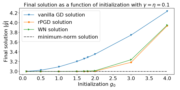
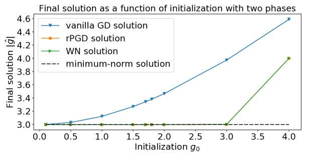
Figure 3: Fixed Orthogonal Matrix $A$. Comparison of the final solutions $|\widehat{g}|=\|\widehat{g}\widehat{w}\|=||\widehat{x}||$ provided by GD, WN and our proposed rPGD on an overparameterized linear regression problem $\min_{x}\frac{1}{2}\|Ax-y\|_{2}^{2}$. All algorithms start from the same initialization $x_{0}=g_{0}w_{0}$. Compared to GD, WN and rPGD converge to the minimum $\ell_{2}$-norm solution for a larger region of initialization. Top plot is when we use the same stepsize for $w$ and $g$: $\gamma_{t}=\eta_{t}=0.1$. Bottom plot is when we use a particularly small stepsize for $g$ and optimal stepsize for $w$. This implies that a small stepsize for $g$ can arrive to a solution that is close to the minimum-norm solution for even wider range of $g_{0}$.

Let $w_{0}$ be a random unit norm vector. We run the standard gradient descent (GD) algorithm on the problem 1 with the initialization $x_{0}=g_{0}w_{0}$. We run Algorithm 1 and 2 starting from the same initialization, and plot $|\widehat{g}|=\|\widehat{g}\widehat{w}\|_{2}$ as a function of $g_{0}$. We run all of the algorithms until the squared loss satisfies $f(\widehat{w},\widehat{g})\leq 10^{-5}$, where the final solution is denoted as $\widehat{g}\widehat{w}$. We have the following observations:

Figure 1 shows the result when we set a very small but equal learning rate for $w$ and $g$: $\eta_{t}=\gamma_{t}=0.005$. It shows there is no difference between WN and rPGD when the learning rate is small, which matches Lemma 2.2. We can see that both WN and rPGD can get close to the minimum norm solution with a large range of initializations ($g^{*}w^{*}$ for $g_{0}\lessapprox 1.5$) while this is only true for GD when $g_{0}$ is close to $0$. This experiment supports our theory.

The top plot in Figure 3 shows the result when we set relatively large learning rates of $w$ and $g$: $\eta_{t}=\gamma_{t}=0.1$, as in practice where we use the same non-vanishing learning rate for all the layers when training deep neural networks. The plot shows a difference between WN and rPGD when $g_{0}>2$, while the two perform similarly when $g_{0}<2$.

The bottom plot in Figure 3 is when we set (1) WN $\eta_{t}=\|w_{t}\|/(g_{t}^{2}\lambda_{\max})$ for $w$ and $\gamma_{t}=0.005$ for $g$; (2) rPGD $\eta_{t}=1/(g_{t}^{2}\lambda_{\max})$ and $\gamma_{t}=0.005$. This mimics the two-phase algorithm as shown in Theorem 3.2. We can arrive at a solution close to the minimum norm solution for even wider range of $g_{0}\lessapprox 3$.

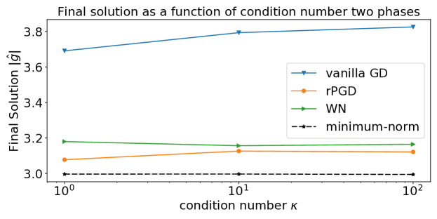
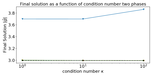
Figure 4: Various General Matrix $A$. Fix $g_{0}=2.8$ and increase the condition number $\kappa$. Top plot: $\gamma_{t}=\eta_{t}=0.01$. The $\ell_{2}$-norm of the WN and rPGD solutions increases slowly as $\kappa$ increases, but their norm is smaller than when using Gradient Descent. Bottom plot: $\gamma_{t}=1,\eta_{t}=0.1\times\mathbb{1}_{\{t>5000\}}$. The $\ell_{2}$-norm of WN and rPGD solutions are robust to condition number and close to the minimum $\ell_{2}$-norm for any $\kappa$. Note that green, orange and black curves of the bottom plot overlap.

Robustness to the condition number $\kappa$. We repeat the previous experiment for various input matrix $A$ with a wider range of $\kappa$ with fixed initialization $g_{0}=2.8$. The top plot in Figure 4 shows that for $\gamma_{t}=\eta_{t}$ as $\kappa$ increases, the $\ell_{2}$-norm of the solutions provided by WN and rPGD also gradually increases but not as much as those provided by the vanilla GD. The bottom plot in Figure 4 shows that the performance of the two-phase algorithms, with $\eta_{t}=0$ in the first 5000 iterations, thus have a better performance compared with algorithm using $\gamma_{t}=\eta_{t}$.

F.2 Experiment: Matrix Sensing

We show that the normalization methods can also be applied to the matrix sensing problem, to get closer to the minimum nuclear norm solutions. The goal in the matrix sensing problem is to recover a low-rank matrix from a small number of random linear measurements. Here we follow the setup considered in Li et al. [2018] (for more related work on matrix sensing and completion, see, e.g., Candès and Recht [2009], Donoho et al. [2013], Ge et al. [2016] and references therein). Let $X^{*}=U^{*}U^{{}^{*}T}\in\mathbb{R}^{d\times d}$ (with $U^{*}\in\mathbb{R}^{d\times r}$) be the ground-truth rank-$r$ matrix. Let $A_{1},..,A_{m}\in\mathbb{R}^{d\times d}$ be $m$ random sensing matrices, with each entry sampled from a standard Gaussian distribution. We are interested in the setting when $r\ll d$ and $m\ll d^{2}$. Given $m$ linear measurements of the form $\left\langle A_{i},X^{*}\right\rangle$, let $U\in\mathbb{R}^{d\times d}$ be the variable matrix, we define the (over-parameterized) loss function as

$$f(U)=\frac{1}{2m}\sum_{i=1}^{m}(\left\langle A_{i},UU^{T}\right\rangle-\left\langle A_{i},X^{*}\right\rangle)^{2}.$$ (53)

It is proved in Li et al. [2018] that if $m=\tilde{O}(dr^{2})$, then gradient descent on $f(U)$, when initialized very close to the origin, can recover the low-rank matrix $X^{*}$.

WN.

To apply WN, we need to reparametrize $U$ into a direction variable and a scale variable. We consider two choices:

• Let $UU^{T}=g\frac{WW^{T}}{\|W\|_{F}^{2}}$, where $g\in\mathbb{R}$, and $W\in\mathbb{R}^{d\times d}$. In Figure 5, the green curve represents this algorithm. We label it with WN.

• Let $UU^{T}=WDW^{T}$, where $D\in\mathbb{R}^{d\times d}$ is a diagonal matrix, and all the column vectors of $W\in\mathbb{R}^{d\times d}$ have unit $\ell_{2}$ norm. That is, for $w_{i}\in\mathbb{R}^{d},i=1,2,\ldots,d$

  $$W=\left[\frac{w_{1}}{\|w_{1}\|};\frac{w_{2}}{\|w_{2}\|};\ldots;\frac{w_{d}}{\|w_{d}\|}\right].$$

  In Figure 5, the purple curve represents the algorithm. We label it with WN-Diag where “Diag" references the diagonal matrix.

rPGD.

To apply rPGD , we need to reparametrize $U$ into a direction variable and a scale variable. We consider two choices:

• Let $UU^{T}=gWW^{T}$, where $g\in\mathbb{R}$, and $W\in\mathbb{R}^{d\times d}$ satisfies $\|W\|_{F}=1$. See Algorithm 3. In Figure 5, the orange curve represents the algorithm. We label it with rPGD.

• Let $UU^{T}=WDW^{T}$, where $D\in\mathbb{R}^{d\times d}$ is a diagonal matrix, and all the column vectors of $W\in\mathbb{R}^{d\times d}$ are projected to have unit $\ell_{2}$ norm. See Algorithm 4. In Figure 5, the red curve represents the algorithm. We label it with rPGD-Diag.

  Input: initialization $W_{0}$ and $g_{0}$, number of iterations $T$, step-sizes $\gamma_{t}$ and $\eta_{t}$.

  for $t=0,1,2,\cdots,T-1$ do

     $V_{t}=W_{t}-\eta_{t}\nabla_{W}f(W_{t},g_{t})$

     $W_{t+1}=\frac{V_{t}}{\|V_{t}\|_{F}}$

     $g_{t+1}=g_{t}-\gamma_{t}\nabla_{g}f(W_{t},g_{t})$

  end for

Algorithm 3 rPGD for matrix sensing loss $f(W,g)$

  Input: initialization $W_{0}$ and $D_{0}$, number of iterations $T$, step-sizes $\gamma_{t}$ and $\eta_{t}$.

  for $t=0,1,2,\cdots,T-1$ do

     $V_{t}=W_{t}-\eta_{t}\nabla_{W}f(W_{t},D_{t})$

     $W_{t+1}=V_{t}$ with all column vectors normalized.

     diag($D_{t+1}$) = diag($D_{t}$) $-\gamma_{t}$ diag($\nabla_{D}f(W_{t},D_{t})$)

  end for

Algorithm 4 rPGD-Diag for matrix sensing loss $f(W,D)$

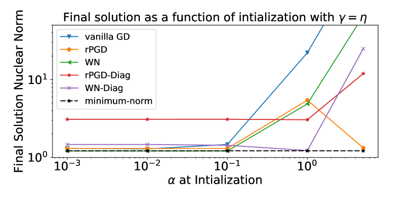
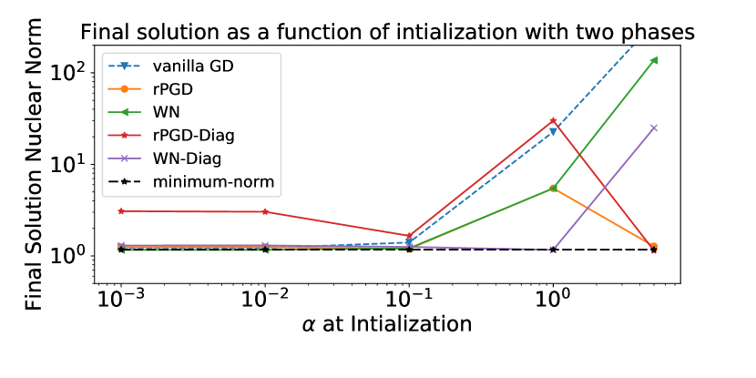
Figure 5: Comparison of the final solutions $\|\widehat{X}\|_{*}$ provided by GD, WN, and rPGD on an overparameterized matrix sensing problem ((53)). All algorithms start from the same initialization with the scale $\alpha=\sqrt{\|UU^{\top}\|_{F}}$. Compared to GD, WN and rPGD converge close to the minimum nuclear-norm solution for a broader region of initialization. The left plot is when we use the same stepsize for $W$ and $g$: $\gamma_{t}=\eta_{t}=c$. The right plot is when we use $\eta_{t}=c$ and $\gamma_{t}=c\mathbb{1}_{\{t>1000\}}$. This suggests that Two-phase algorithm can arrive to a solution closer to the nuclear-norm solution for a broader range of $g_{0}$. The blue, green, and black curves of the top plot overlap when $0<\alpha<0.1$. The blue, orange, green, purple, and black curves of the bottom plot overlap when $0<\alpha<0.1$.

Denote the corresponding loss functions for rPGD as $f(W,g)$ and $f(W,D)$. Let $Z_{0}=Z/\|Z\|_{F}$ where $Z$ is a matrix with i.i.d. Gaussian entries, after which all column vectors have been normalized. We set the experiments with the following initialization:

• For vanilla GD on $f(U)$, let $U_{0}=\alpha Z_{0}$;

• For WN and rPGD, let $W_{0}=Z_{0}$, and $g_{0}=\alpha^{2}$ ;

• For WN-Diag and rPGD-Diag, let $W_{0}=Z_{0}$ and $D_{0}=\alpha^{2}I$.

We set $d=30$, $r=4$, and $m=60$. We simulate $y_{i}=\langle{A_{i},\hat{U}\hat{U}\rangle}$ with $\hat{U}\in\mathbb{R}^{d\times r}$ generated as a random matrix.

We compare the performance of gradient descent, and our algorithms for several initializations scales $g$. We run each algorithm until convergence (i.e., when the squared loss is less than $10^{-6}$).

Similar to Figure 3, we use different learning rate schemes to get the final solution. We use grid search to find appropriate constant learning rate c. The top plot in Figure 5 uses the following learning rate: constant $c$ for gradient descent; $\eta_{t}=\gamma_{t}=c$ for rPGD (Algorithm 3 and 4); and set $\eta_{t}=\gamma_{t}=c\|W\|_{F}$ for WN. The bottom plot in Figure 5 uses the two phase learning rates: constant for gradient descent; $\eta_{t}=c$ and $\gamma_{t}=c\mathbf{1}_{\{t>1000\}}$ for rPGD (Algorithm 3 and 4); and set $\eta_{t}=\gamma_{t}=c\|W\|_{F}$ and $\gamma_{t}=c\mathbb{1}_{\{t>1000\}}$ for WN. Compared to GD, WN and rPGD converge close to the minimum nuclear-norm solution for a larger region of initialization. Moreover, these results also suggest that with the two-phase algorithm, one can arrive to a solution close to the nuclear-norm solution for a wider range of $g_{0}$.

References

- Ali et al. (2018) Alnur Ali, J Zico Kolter, and Ryan J Tibshirani. A continuous-time view of early stopping for least squares regression. arXiv preprint arXiv:1810.10082, 2018.
- Arora et al. (2020) Raman Arora, Peter Bartlett, Poorya Mianjy, and Nathan Srebro. Dropout: Explicit forms and capacity control. arXiv preprint arXiv:2003.03397, 2020.
- Arora et al. (2018) Sanjeev Arora, Zhiyuan Li, and Kaifeng Lyu. Theoretical analysis of auto rate-tuning by batch normalization. arXiv preprint arXiv:1812.03981, 2018.
- Arora et al. (2019) Sanjeev Arora, Nadav Cohen, Wei Hu, and Yuping Luo. Implicit regularization in deep matrix factorization. arXiv preprint arXiv:1905.13655, 2019.
- Ba et al. (2016) Jimmy Lei Ba, Jamie Ryan Kiros, and Geoffrey E Hinton. Layer normalization. arXiv preprint arXiv:1607.06450, 2016.
- Bartlett et al. (2019) Peter L Bartlett, Philip M Long, Gábor Lugosi, and Alexander Tsigler. Benign overfitting in linear regression. arXiv preprint arXiv:1906.11300, 2019.
- Belkin et al. (2019) Mikhail Belkin, Daniel Hsu, and Ji Xu. Two models of double descent for weak features. arXiv preprint arXiv:1903.07571, 2019.
- Cai et al. (2019) Yongqiang Cai, Qianxiao Li, and Zuowei Shen. A quantitative analysis of the effect of batch normalization on gradient descent. In International Conference on Machine Learning, pages 882–890, 2019.
- Candès and Recht (2009) Emmanuel J Candès and Benjamin Recht. Exact matrix completion via convex optimization. Foundations of Computational mathematics, 9(6):717, 2009.
- Chen et al. (2019) Shuxiao Chen, Edgar Dobriban, and Jane H Lee. Invariance reduces variance: Understanding data augmentation in deep learning and beyond. arXiv preprint arXiv:1907.10905, 2019.
- Dobriban and Wager (2018) Edgar Dobriban and Stefan Wager. High-dimensional asymptotics of prediction: Ridge regression and classification. The Annals of Statistics, 46(1):247–279, 2018.
- Donoho et al. (2013) David L Donoho, Matan Gavish, and Andrea Montanari. The phase transition of matrix recovery from gaussian measurements matches the minimax mse of matrix denoising. Proceedings of the National Academy of Sciences, 110(21):8405–8410, 2013.
- Douglas et al. (2000) Scott C Douglas, Shun-ichi Amari, and S-Y Kung. On gradient adaptation with unit-norm constraints. IEEE Transactions on Signal Processing, 48(6):1843–1847, 2000.
- Du et al. (2018) Simon S Du, Xiyu Zhai, Barnabas Poczos, and Aarti Singh. Gradient descent provably optimizes over-parameterized neural networks. arXiv preprint arXiv:1810.02054, 2018.
- Dukler et al. (2020) Yonatan Dukler, Guido Montufar, and Quanquan Gu. Optimization theory for relu neural networks trained with normalization layers. In Proceedings of the 37th International Conference on Machine Learning, 2020.
- Gal and Ghahramani (2016) Yarin Gal and Zoubin Ghahramani. Dropout as a bayesian approximation: Representing model uncertainty in deep learning. In international conference on machine learning, pages 1050–1059, 2016.
- Ge et al. (2016) Rong Ge, Jason D Lee, and Tengyu Ma. Matrix completion has no spurious local minimum. In Advances in Neural Information Processing Systems, pages 2973–2981, 2016.
- Ge et al. (2017) Rong Ge, Chi Jin, and Yi Zheng. No spurious local minima in nonconvex low rank problems: A unified geometric analysis. In International Conference on Machine Learning, pages 1233–1242, 2017.
- Glorot and Bengio (2010) Xavier Glorot and Yoshua Bengio. Understanding the difficulty of training deep feedforward neural networks. In Proceedings of the thirteenth international conference on artificial intelligence and statistics, pages 249–256, 2010.
- Goyal et al. (2017) Priya Goyal, Piotr Dollár, Ross Girshick, Pieter Noordhuis, Lukasz Wesolowski, Aapo Kyrola, Andrew Tulloch, Yangqing Jia, and Kaiming He. Accurate, large minibatch sgd: Training imagenet in 1 hour. arXiv preprint arXiv:1706.02677, 2017.
- Gunasekar et al. (2017) Suriya Gunasekar, Blake E Woodworth, Srinadh Bhojanapalli, Behnam Neyshabur, and Nati Srebro. Implicit regularization in matrix factorization. In Advances in Neural Information Processing Systems, pages 6151–6159, 2017.
- Gunasekar et al. (2018) Suriya Gunasekar, Jason Lee, Daniel Soudry, and Nathan Srebro. Characterizing implicit bias in terms of optimization geometry. arXiv preprint arXiv:1802.08246, 2018.
- Hastie et al. (2019) Trevor Hastie, Andrea Montanari, Saharon Rosset, and Ryan J Tibshirani. Surprises in high-dimensional ridgeless least squares interpolation. arXiv preprint arXiv:1903.08560, 2019.
- Hayes (2009) Monson H Hayes. Statistical digital signal processing and modeling. John Wiley & Sons, 2009.
- Haykin (2005) Simon S Haykin. Adaptive filter theory. Pearson Education India, 2005.
- Haykin and Widrow (2002) Simon Saher Haykin and Bernard Widrow. Least-mean-square adaptive filters. Citeseer, 2002.
- He et al. (2015) Kaiming He, Xiangyu Zhang, Shaoqing Ren, and Jian Sun. Delving deep into rectifiers: Surpassing human-level performance on imagenet classification. In Proceedings of the IEEE international conference on computer vision, pages 1026–1034, 2015.
- Helmke and Moore (2012) Uwe Helmke and John B Moore. Optimization and dynamical systems. Springer Science & Business Media, 2012.
- Hoffer et al. (2018) Elad Hoffer, Ron Banner, Itay Golan, and Daniel Soudry. Norm matters: efficient and accurate normalization schemes in deep networks. In Advances in Neural Information Processing Systems, pages 2160–2170, 2018.
- Ioffe and Szegedy (2015) Sergey Ioffe and Christian Szegedy. Batch normalization: Accelerating deep network training by reducing internal covariate shift. arXiv preprint arXiv:1502.03167, 2015.
- Jacot et al. (2018) Arthur Jacot, Franck Gabriel, and Clément Hongler. Neural tangent kernel: Convergence and generalization in neural networks. In Advances in neural information processing systems, pages 8571–8580, 2018.
- Ji and Telgarsky (2019) Ziwei Ji and Matus Telgarsky. The implicit bias of gradient descent on nonseparable data. In Conference on Learning Theory, pages 1772–1798, 2019.
- Kohler et al. (2019) Jonas Kohler, Hadi Daneshmand, Aurelien Lucchi, Thomas Hofmann, Ming Zhou, and Klaus Neymeyr. Exponential convergence rates for batch normalization: The power of length-direction decoupling in non-convex optimization. In AISTATS, pages 806–815, 2019.
- LeCun et al. (2015) Yann LeCun, Yoshua Bengio, and Geoffrey Hinton. Deep learning. nature, 521(7553):436–444, 2015.
- Lee et al. (2019) Jaehoon Lee, Lechao Xiao, Samuel Schoenholz, Yasaman Bahri, Roman Novak, Jascha Sohl-Dickstein, and Jeffrey Pennington. Wide neural networks of any depth evolve as linear models under gradient descent. In Advances in neural information processing systems, pages 8570–8581, 2019.
- Lee et al. (2016) Jason D Lee, Max Simchowitz, Michael I Jordan, and Benjamin Recht. Gradient descent converges to minimizers. arXiv preprint arXiv:1602.04915, 2016.
- Li et al. (2018) Yuanzhi Li, Tengyu Ma, and Hongyang Zhang. Algorithmic regularization in over-parameterized matrix sensing and neural networks with quadratic activations. In Conference On Learning Theory, pages 2–47. PMLR, 2018.
- Lian and Liu (2019) Xiangru Lian and Ji Liu. Revisit batch normalization: New understanding and refinement via composition optimization. In Kamalika Chaudhuri and Masashi Sugiyama, editors, Proceedings of Machine Learning Research, volume 89 of Proceedings of Machine Learning Research, pages 3254–3263, 16–18 Apr 2019.
- Liang and Rakhlin (2018) Tengyuan Liang and Alexander Rakhlin. Just interpolate: Kernel "ridgeless" regression can generalize. arXiv preprint arXiv:1808.00387, 2018.
- Liu and Dobriban (2019) Sifan Liu and Edgar Dobriban. Ridge regression: Structure, cross-validation, and sketching. arXiv preprint arXiv:1910.02373, 2019.
- Luo et al. (2019) Ping Luo, Xinjiang Wang, Wenqi Shao, and Zhanglin Peng. Towards understanding regularization in batch normalization. In International Conference on Learning Representations, 2019.
- Mahoney and Martin (2019) Michael Mahoney and Charles Martin. Traditional and heavy tailed self regularization in neural network models. In International Conference on Machine Learning, pages 4284–4293, 2019.
- Mahoney (2012) Michael W Mahoney. Approximate computation and implicit regularization for very large-scale data analysis. In Proceedings of the 31st ACM SIGMOD-SIGACT-SIGAI symposium on Principles of Database Systems, pages 143–154. ACM, 2012.
- Martin and Mahoney (2018) Charles H Martin and Michael W Mahoney. Implicit self-regularization in deep neural networks: Evidence from random matrix theory and implications for learning. arXiv preprint arXiv:1810.01075, 2018.
- Mianjy et al. (2018) Poorya Mianjy, Raman Arora, and Rene Vidal. On the implicit bias of dropout. arXiv preprint arXiv:1806.09777, 2018.
- Morgan and Bourlard (1990) Nelson Morgan and Hervé Bourlard. Generalization and parameter estimation in feedforward nets: Some experiments. In Advances in neural information processing systems, pages 630–637, 1990.
- Neyshabur et al. (2014) Behnam Neyshabur, Ryota Tomioka, and Nathan Srebro. In search of the real inductive bias: On the role of implicit regularization in deep learning. arXiv preprint arXiv:1412.6614, 2014.
- Neyshabur et al. (2019) Behnam Neyshabur, Zhiyuan Li, Srinadh Bhojanapalli, Yann LeCun, and Nathan Srebro. The role of over-parametrization in generalization of neural networks. In International Conference on Learning Representations, 2019. URL https://openreview.net/forum?id=BygfghAcYX.
- Poggio et al. (2019) Tomaso Poggio, Andrzej Banburski, and Qianli Liao. Theoretical issues in deep networks: Approximation, optimization and generalization. arXiv preprint arXiv:1908.09375, 2019.
- Proakis (2001) John G Proakis. Digital signal processing: principles algorithms and applications. Pearson Education India, 2001.
- Rockafellar and Wets (2009) R Tyrrell Rockafellar and Roger J-B Wets. Variational analysis, volume 317. Springer Science & Business Media, 2009.
- Salimans and Kingma (2016) Tim Salimans and Diederik P Kingma. Weight normalization: A simple reparameterization to accelerate training of deep neural networks. In Advances in Neural Information Processing Systems, pages 901–909, 2016.
- Santurkar et al. (2018) Shibani Santurkar, Dimitris Tsipras, Andrew Ilyas, and Aleksander Madry. How does batch normalization help optimization? In Advances in Neural Information Processing Systems, pages 2483–2493, 2018.
- Soudry et al. (2018) Daniel Soudry, Elad Hoffer, Mor Shpigel Nacson, Suriya Gunasekar, and Nathan Srebro. The implicit bias of gradient descent on separable data. The Journal of Machine Learning Research, 19(1):2822–2878, 2018.
- Strand (1974) Otto Neall Strand. Theory and methods related to the singular-function expansion and landweber’s iteration for integral equations of the first kind. SIAM Journal on Numerical Analysis, 11(4):798–825, 1974.
- Strohmer and Vershynin (2009) Thomas Strohmer and Roman Vershynin. A randomized kaczmarz algorithm with exponential convergence. Journal of Fourier Analysis and Applications, 15(2):262, 2009.
- Tian (2019) Yuandong Tian. Over-parameterization as a catalyst for better generalization of deep relu network. arXiv preprint arXiv:1909.13458, 2019.
- Tian et al. (2019) Yuandong Tian, Tina Jiang, Qucheng Gong, and Ari Morcos. Luck matters: Understanding training dynamics of deep relu networks. arXiv preprint arXiv:1905.13405, 2019.
- Ulyanov et al. (2016) Dmitry Ulyanov, Andrea Vedaldi, and Victor Lempitsky. Instance normalization: The missing ingredient for fast stylization. arXiv preprint arXiv:1607.08022, 2016.
- Vaškevičius et al. (2019) Tomas Vaškevičius, Varun Kanade, and Patrick Rebeschini. Implicit regularization for optimal sparse recovery. arXiv preprint arXiv:1909.05122, 2019.
- Vershynin (2018) Roman Vershynin. High-dimensional probability: An introduction with applications in data science, volume 47. Cambridge University Press, 2018.
- Wager et al. (2013) Stefan Wager, Sida Wang, and Percy S Liang. Dropout training as adaptive regularization. In Advances in neural information processing systems, pages 351–359, 2013.
- Ward et al. (2019) Rachel Ward, Xiaoxia Wu, and Leon Bottou. AdaGrad stepsizes: Sharp convergence over nonconvex landscapes. In Proceedings of the 36th International Conference on Machine Learning, pages 6677–6686, 09–15 Jun 2019.
- Wu et al. (2018) Xiaoxia Wu, Rachel Ward, and Léon Bottou. Wngrad: learn the learning rate in gradient descent. arXiv preprint arXiv:1803.02865, 2018.
- Xu et al. (2019) Jingjing Xu, Xu Sun, Zhiyuan Zhang, Guangxiang Zhao, and Junyang Lin. Understanding and improving layer normalization. In Advances in Neural Information Processing Systems, pages 4383–4393, 2019.
- Zhang et al. (2016) Chiyuan Zhang, Samy Bengio, Moritz Hardt, Benjamin Recht, and Oriol Vinyals. Understanding deep learning requires rethinking generalization. arXiv preprint arXiv:1611.03530, 2016.